Closing the Gap between Deep Neural Network Modeling and Biomedical Decision-Making Metrics in Segmentation via Adaptive Loss Functions

Abstract

Deep learning is becoming an indispensable tool for various tasks in science and engineering. A critical step in constructing a reliable deep learning model is the selection of a loss function, which measures the discrepancy between the network prediction and the ground truth. While a variety of loss functions have been proposed in the literature, a truly optimal loss function that maximally utilizes the capacity of neural networks for deep learning-based decision-making has yet to be established. Here, we devise a generalized loss function with functional parameters determined adaptively during model training to provide a versatile framework for optimal neural network-based decision-making in small target segmentation. The method is showcased by more accurate detection and segmentation of lung and liver cancer tumors as compared with the current state-of-the-art. The proposed formalism opens new opportunities for numerous practical applications such as disease diagnosis, treatment planning, and prognosis.

I. INTRODUCTION

DECISION-making using deep learning models has recently gained enormous momentum in science and engineering and found important applications in disciplines such as computer vision [1, 2], natural language processing [3], and biomedicine [4–8]. In deep learning, a neural network learns from a large set of training data by means of a loss function, which guides the search for optimal network parameters by quantifying how accurately the network models the training data. Similar to any optimization problem [9], there is generally no one-size-fits-all loss function for training deep learning algorithms and various forms of loss function have been proposed for different or even the same applications. In practice, a loss function is constructed by accounting for multiple factors that impact the learning and evaluation processes, including computational efficiency, optimization algorithm, and nature of training and test datasets.

An important but less appreciated issue with the current paradigm is that minimizing a pre-defined loss function alone does not always yield truly optimal prediction. Indeed, the assumption in the current machine learning paradigm according to which handcrafting a fixed loss function ahead of training is a good proxy for an underlying metric of interest evaluated post-training is often violated. First, the nonlinear combination of a large number of parameters in deep neural networks leads to highly non-convex loss functions, which are difficult to optimize robustly with simple gradient-based methods theoretically designed for convex problems. For instance, stochastic gradient method, which is commonly used for neural network optimization, may not be stable in some scenarios [10]. In reality, while all loss functions reduce the multi-dimensional representation of a neural network to a single number for inference, it is important to note that some number is better than others and the essence here is to find the loss function which generate a number that is most consistent with our final decision-making metric. We note that the primary building blocks of classification evaluation metrics - true positive (TP) and false negative (FN) for positive-class examples correctly and incorrectly predicted by the model, respectively, and their two negative-class counterparts, true negative (TN) and false positive (FP) - can be combined into a scalar loss function that more meaningfully aligns with the decision-making metrics in multiple ways. For example, a popular and largely used metric for semantic segmentation tasks is the Dice similarity coefficient, harmonic mean of precision (P = TP/[TP + FP]) and recall (R = TP/[TP + FN]). However, although it partially accounts for imbalance typically related to low prevalence of pixels with positive class in individual images, it does not always lead to a truly optimal model prediction and significant bottlenecks remain [11–14]. In light of the two aforementioned pitfalls, constructing a loss function that meaningfully reduces the multi-dimensional representation of a neural network to a differentiable scalar function that can be optimized via traditional gradient-based algorithms is a challenging task.

The present study aims to mitigate the above issues and close the gap between deep neural network modeling and decision-making metrics. Our strategy consists of exploiting a flexible parameterization of the loss function via a generalized formulation whose parameters are adaptively tuned during regular training. In particular, we demonstrate how a three-dimensional parameterization of the Dice coefficient leads to a generalized loss function that allows for greater flexibility in the relative weighting of relevant decision-making metrics. Additionally, we propose two adaptive strategies for evolving the optimal loss function to reduce the mismatch between loss function and decision-making metrics during model training. In particular, we detail a mathematically motivated adaptive strategy that does not introduce any computational overhead and can be easily plugged in most deep learning frameworks. In application to cancer tumor detection and segmentation, the new paradigm yields improved performance as compared with the current state-of-the-art by up to 10%.

II. Methods

A. Generalized loss function and adaptive training methodology

We propose a new generalized loss function (GLF)

$$\mathcal{G}=1-\frac{1+{\beta }^2}{\frac{1}{P_{{\alpha }_P}}+\frac{{\beta }^2}{R_{{\alpha }_N}}}.$$ (1)

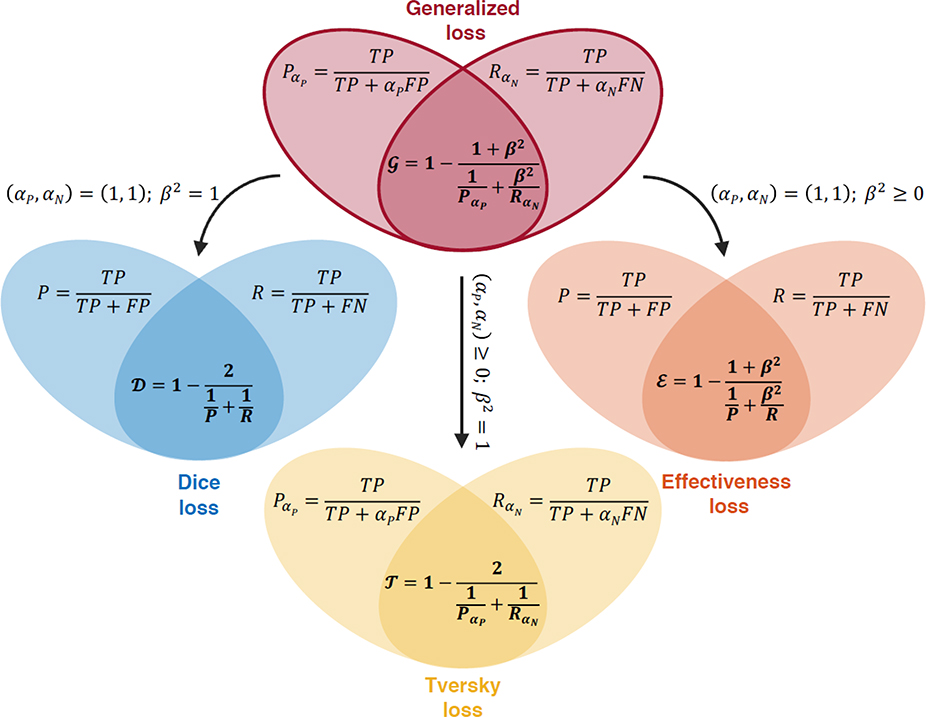
A descriptive schematic of this new loss function $\mathcal{G}$ is depicted in Fig. 1. The formulation involves three coefficients α_P, α_N, and β² that are reminiscent of the coefficients appearing in the Effectiveness and Tversky loss functions [13, 14]. The GLF uses all three coefficients simultaneously in a way that enables independent pairwise weighting of the relevant decision-making metrics. The coefficients α_P, α_N, and β² control the relative weighting between TP and FP, TP and FN, and $P_{{\alpha }_P}$ and $R_{{\alpha }_N}$, respectively. Therefore, the coefficients α_P and α_N play a similar role as the Tversky constants in defining weighted precision $P_{{\alpha }_P}$ and weighted recall $R_{{\alpha }_N}$, while the coefficient β² is analogous to the Effectiveness constant in weighting the harmonic mean of these two quantities instead of the arithmetic mean. The harmonic mean was chosen because of its appropriateness when the combination of adversarial metrics is used to evaluate segmentation tasks [15]. Besides the conventional Tversky and Effectiveness loss functions, a number of alternative formulations have been proposed that, however, similarly rely on manual hyperparameter tuning and involve complex formulations [16–21].

Fig. 1.

Definition of the generalized loss function and schematic of its relationships to conventional Dice, Effectiveness and Tversky loss functions. The definition of the generalized loss function involves three coefficients α_P, α_N, and β². For specific values of these coefficients, the generalized loss function collapses to conventional loss functions.

As shown in Fig. 1, the conventional Dice, Tversky and Effectiveness loss functions can be derived from the generalized formulation when the coefficients take on specific constant values. The Dice loss is recovered when (α_P, α_N) = (1,1) and β² = 1, which encodes for unweighted harmonic mean of unweighted precision and recall. The Effectiveness loss is obtained when (α_P, α_N) = (1,1) with β² ≥ 0, which corresponds to the weighted harmonic mean between unweighted precision and recall. Finally, the GLF collapses to the Tversky loss when β² = 1 with (α_P, α_N) ≥ 0, which corresponds to the unweighted harmonic mean between weighted precision and recall. It is worthwhile to note that the Dice loss function is a special case of the Effectiveness loss function, which is itself a special case of the Tversky loss function. Indeed, the Effectiveness loss function can be rearranged as the unweighted harmonic mean between weighted precision and weighted recall, where the weights in $P_{{\alpha }_P}$ and $R_{{\alpha }_N}$ sum to two. The GLF formulation allows for more flexibility in weighting the relative importance of the different metrics in the loss. Thus, the GLF value ranks a possible solution more objectively through an adaptive combination of multi-dimensional information.

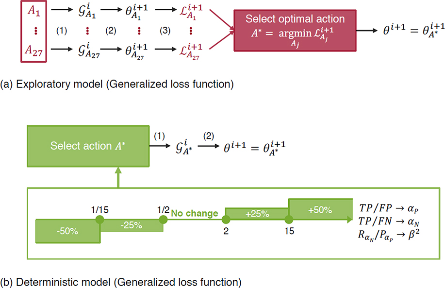
With the conventional a priori tuning of the hyperparameters in the loss, the performance of the trained neural networks would be highly sensitive to the choice of the hyperparameters and they would require careful manual tuning in practice [13, 14]. Instead of adopting the conventional a priori tuning for the GLF coefficients, we propose an adaptive procedure to automatically evolve the coefficients at every optimization iteration during the training of the network as well. With this adaptive training method, only one simulation is run, and the loss coefficients adaptively determine the optimal loss during the training. At every iteration, there is a discrete set of possible actions for each parameter that is picked either based on a greedy algorithm, or deterministic heuristics that are motivated by a simple mathematical analysis of the loss function. Both approaches are concisely described in Fig. 2 and are detailed in the Methods section. It is noteworthy that the deterministic approach does not introduce computational overhead and can be easily incorporated in most existing deep learning frameworks.

Fig. 2.

Adaptive training methodologies for the coefficients in the Generalized loss function. (a) Exploratory model where all possible actions (−10%, no change, +10%) are explored at each iteration step for each of the three parameters, and the action triplet yielding the best performance $(\underset{A_j}{argmin}{\mathcal{L}}_{Aj}^{i+1})$ is picked. (b) Deterministic model based on rule-based update formula for the three coefficients that can each take one of five possible actions. For example, α_P decreases by a factor of 50% if TP/FP is smaller than 1/15. In order to avoid the unbounded divergence of the parameters, the parameters α_P and α_N are not updated when <FP> ≤5 and <FN> ≤ 1, respectively, where the symbols <·> denote batch-averaged values.

B. Adaptive hyperparameter tuning methods

Conventional methods regard the coefficients in the loss function as fixed hyperparameters. It is well known that the performance of deep learning modeling is highly sensitive to the choice of these hyperparameters, e.g. for semantic segmentation [13], imbalanced classification, image reconstruction, and multi-task learning. Therefore, the coefficients are typically manually tuned and kept constant during the entire neural network training. Hyperparameter values that yield the best metric performance are prospectively picked as the optimal parameters. This is a computationally expensive procedure that relies on a time-consuming trial-and-error human intervention. Furthermore, the conventional practice of manually tuning the hyperparameters a priori assumes that the optimal choice of the coefficients remains constant throughout the training phase, which inevitably leads to suboptimal or even erroneous results as shown below.

The first adaptive method (exploratory) loosens the above restriction by allowing each coefficient to take one of three possible actions: decrease by 10%, keep constant, or increase by 10%. Since there are three parameters, this yields a total of 27 possible actions A₁ up to A₂₇ at every iteration step i of the backpropagation algorithm. Each action A_j corresponds to a new instance of the generalized loss ${\mathcal{G}}_{A_j}^i$ and is explored by the algorithm that backpropagates once with this loss to update the network parameters ${\theta }_{A_j}^{i+1}$ at the next iteration step. The performance criterion used to evaluate each action is the batch-averaged Euclidian distance ${\mathcal{L}}_{A_j}^{i+1}$ between prediction and ground-truth label. The greedy action $A^{*}=\underset{A_j}{\mathrm{argmin}}{\mathcal{L}}_{Aj}^{i+1}$ is then selected to decide the optimal update rule for the GLF coefficients, and the final network parameters are updated as ${\theta }^{i+1}={\theta }_{A^{*}}^{i+1}$. The first approach is exploratory in nature and increases the computational cost of training the neural network. However, it allows to assess the relevance of the adaptive training concept for the loss coefficients. It is a viable approach in applications where deep neural network training time is not the bottleneck. An alternative refined algorithm would consist in training a reinforcement learning algorithm to learn the optimal update rule, with a policy parameterized as a deep neural network and every iteration stage considered a state.

The second adaptive approach (deterministic) consists in updating each coefficient via a deterministic rule that outputs one of five possible actions: decrease by 50%, decrease by 25%, keep constant, increase by 25%, or increase by 50%. The deterministic rule is motivated by the results obtained with the exploratory rule, from which we have inferred possible heuristics that explain the dynamic change of the coefficients. Since gradient-based optimizers primarily rely on the first-order gradient information [22–28], we mathematically analyze the gradients of the GLF with respect to the network parameters, which can be formulated as

$$\frac{\nabla (1-\mathcal{G})}{1-\mathcal{G}}=\frac{1}{\frac{1}{P_{{\alpha }_P}}+\frac{{\beta }^2}{R_{{\alpha }_N}}}\left(\frac{\nabla P_{{\alpha }_P}}{{P_{{\alpha }_P}}^2}+{\beta }^2\frac{\nabla R_{{\alpha }_N}}{{R_{{\alpha }_N}}^2}\right),$$ (2)

where the two gradient terms on the right side can be further decomposed as

$$\nabla P_{{\alpha }_P}=\frac{TP{\alpha }_{P}FP}{{\left(TP+{\alpha }_{P}FP\right)}^2}\left(\frac{\nabla TP}{TP}-\frac{\nabla FP}{FP}\right),$$ (3)

$$\nabla R_{{\alpha }_N}=\frac{TP{\alpha }_{N}FN}{{\left(TP+{\alpha }_{N}FN\right)}^2}\left(\frac{\nabla TP}{TP}-\frac{\nabla FN}{FN}\right).$$ (4)

It is instructive to consider the order of magnitude of the prefactors on the right side of Eq. (3) when the coefficient α_P is of order 1. For example, when FP ≫ TP, the prefactor in Eq. (3) is of the order of TP/FP ≪ 1 (i.e., TP is much smaller than FP). In contrast, when FP ≪ TP, the prefactor is of the order of FP/TP ≪ 1. These results in an artificial attenuation of the learning rate along the TP and FP directions. This can be partially circumvented by adaptively changing α_P to counterbalance the effect: decreasing α_P when FP ≫ TP as typically occurs in early stages of training, and increasing it when TP ≫ FP. A similar interpretation can be made for α_N by considering the right side of Eq. (4). A possible interpretation for β² consists in arguing that the relative weight along the $\nabla P_{{\alpha }_P}/P_{{\alpha }_P}$ and $\nabla R_{{\alpha }_N}/R_{{\alpha }_N}$ directions should be of the same order (as they are in Eq. (3) and Eq. (4) for TP, FP, and FN). The relative weight $\left({\beta }^2{P}_{{\alpha }_P}/R_{{\alpha }_N}\right)$ therefore justifies increasing β² when $P_{{\alpha }_P}\ll R_{{\alpha }_N}$ and decreasing it when $P_{{\alpha }_P}\gg R_{{\alpha }_N}$. The exact heuristics that are picked for each coefficient in this work are shown in Fig. (2b). We hypothesize that the induced dynamic changes minimize the risks for the network to get trapped in a local minimum during training. The rule-based deterministic adaptive does not introduce significant computational overhead as compared with the conventional approaches based on the Dice, Effectiveness or Tversky loss functions.

C. Training details

The 2D segmentation network employed in this study is the modified U-Net (mU-Net) architecture [29] implemented in Tensorflow [30]. In all cases, neural network parameters are randomly initialized using a truncated normal distribution with mean value of 0, standard deviation of 0.05, and constant bias values of 0.1. During training, they are updated using Adam’s optimization algorithm [25]. The initial learning rate is 0.0001. The decay value of the moving average in the batch normalization was 0.9 for regularization and the dropout probability was 0.6 minimize overfitting. During training, the continuous values of the output layer are used to calculate the loss function and its gradient.

Public lung and liver tumor datasets were used [31, 32]. The lung tumor dataset is composed of very small targets in large images (largest tumor size: 0.18 % of the total 512² number of pixels). The liver tumor dataset similarly contains small targets that also have relatively irregular boundaries. Supplementary Table 1¹ shows the breakdown of patients and 2D CT scans into training, validation, and testing datasets. All input images are 512×512 and data processing and analysis are implemented using MATLAB (9.4.0.813654, R2018a, The MathWorks Inc., Matrick, MA). The performance metrics are calculated by thresholding the continuous output layer values with a threshold 0.5.

Throughout the study, we compare the performances of the proposed methods based on the GLF against the results obtained with the Dice, Effectiveness and Tversky loss functions. In the two latter cases, the comparisons are done against the choice of hyperparameters that yield the highest Dice coefficient, in order to make the comparison more robust. The most accurate Effectiveness and Tversky loss functions were found by training a number of neural networks with different choices of the manually tuned hyperparameters. Supplemental Figure 1¹ shows the results of these parametric studies.

The main data supporting the results in this study are available within the paper and its supplementary information¹. The lung and liver tumor datasets are publicly available at https://medicaldecathlon.com and https://competitions.codalab.org/competitions/17094, respectively.

III. Results

The GLF in conjunction with the deterministic (D) and exploratory (E) adaptive training methodologies is applied the detection and segmentation of lung and liver cancer tumors in CT scans. The performances of the two methods are evaluated with delineations from physicians as ground truths.

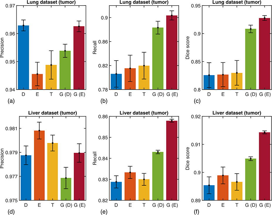
The averaged precision, recall, and Dice coefficient of the two proposed methods are shown in Fig. 3, where they are compared against three conventional methods based on the Dice, Effectiveness, and Tversky loss functions. The precision of the deep learning segmentation algorithm exhibits little sensitivity to the choice of the training loss, with less than 2% and 0.01% difference between the worst and best methods for the lung and liver datasets, respectively. The precision reach very high values up to 96.3% and 98.1%, suggesting that detected tumors are accurately delineated. On the other hand, the recall performance of the algorithms varies significantly by up to 10% depending on the choice of the training loss. In particular, the proposed training methods yield values of 88.3% (D) and 90.4% (E) for the lung dataset, and 84.3% (D) and 85.8% (E) for the liver dataset, all statistically significantly larger compared to the 82% and 83.3% best recall performance obtained with the conventional loss functions. The Dice coefficients, displayed in the rightmost column, show that the new methods overall outperform the existing methods by nearly 10% and 2% for the lung and liver datasets, respectively. The exploratory strategy of the adaptive loss performs slightly better than its deterministic counterpart. This is expected as the deterministic version of the adaptive loss aims at approximating the exploratory loss using simple heuristics. However, it is noteworthy that the results obtained with the deterministic generalized loss function still outperform the existing methods with no computational overhead.

Fig. 3.

Quantitative results for the test data samples that contain at least one tumor. The averaged (a,d) precision, (b,e) recall, and (c,f) Dice coefficients are shown for the lung dataset (upper panel) and liver dataset (lower panel). D, E, T, G (D), and G (E)are results obtained with the Dice loss, Effectiveness loss, Tversky loss, generalized loss based on the deterministic approach, and generalized loss based on exploratory approach, respectively. Numerical values are reported in Supplementary Tables 2 and 4.

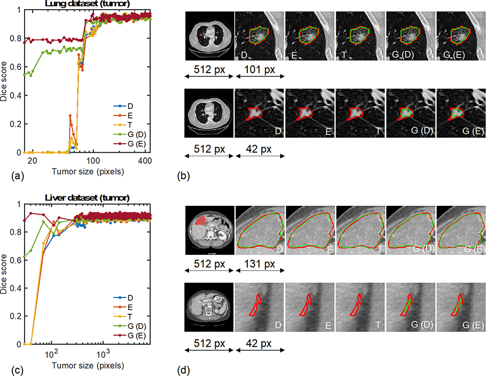
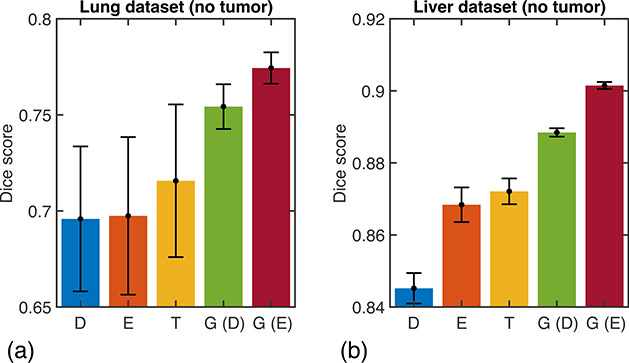
To gain insights into the difference in performance of different methods, Fig. 4(a,c) show the distribution of the Dice coefficient across all tumor sizes encountered in the test datasets. While all methods exhibit similar performance for the largest tumors, significant differences are observed in the small-size tumor range, corresponding to sizes below approximately 100 pixels in both cases (less than 0.04% of the total 512² number of pixels). The adaptive methods based on the GLF are consistently able to detect and segment small-size tumors that would have remained undetected otherwise, increasing the sample wise Dice score from 0% with existing method to well above 50% when the GLF and adaptive training methods are used. This analysis of the accuracy of the methods for various tumor sizes provides insights into their averaged precision and recall metrics discussed above. Indeed, with conventional loss functions and training methodologies, small tumors are not detected and are counted as false negatives, thereby penalizing the recall scores of the methods but with no negative effect on the precision scores. This observation is visually ratified on Fig. 4(b,d) that qualitatively show the segmentation performances of all methods for one small and one intermediate-size tumor in each dataset. While all methods perform equally well for the larger tumors, only the two proposed methods are able to detect and segment the smallest-size tumors. Figure 5 shows the Dice coefficients of the different methodologies in the more special case when the test data samples that do not contain any tumor. The proposed methods outperform the existing methods on both datasets. On the lung (liver) data, the Dice coefficient is increased from 71.6% (87.2%) for the Tversky loss to 75.4% (88.8%) and 77.4% (90.1%) for the deterministic and exploratory training of the GLF, respectively.

Fig. 4.

Segmentation results for the test data samples that contain at least one tumor. Distribution of Dice coefficients across tumor sizes for the (a) lung and (c) liver datasets. Visualizations of the algorithms’ delineations for the (b) lung and (d) liver datasets. In (b) and (d), the top row corresponds to an intermediate-size tumor example while the bottom row corresponds to a small tumor example. For reference for the liver dataset in (d): the full length 512 pixels of the CT scan corresponds to 30cm, the large tumor magnification window length 131px corresponds to 76mm, and the small tumor magnification window length 42 pixels corresponds to 24mm. D, E, T, G (D), and G (E) correspond to the Dice loss, Effectiveness loss, Tversky loss, generalized loss based on deterministic approach, and generalized loss based on exploratory approach, respectively.

Fig. 5.

Quantitative results for the test data samples that do not contain any tumor. The averaged Dice coefficient is shown for the (a) lung and (b) liver datasets. D, E, T, G (D), and G (E) refer to the Dice loss, Effectiveness loss, Tversky loss, generalized loss based on deterministic approach, and generalized loss based on exploratory approach, respectively. Numerical values are reported in Supplementary Tables 3 and 5.

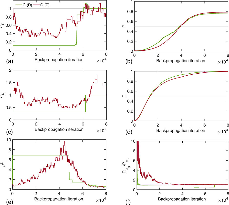
The improvement in predictive capability of the deep learning model owes to the adaptive training strategy that enables the GLF to be automatically tuned during the training process of the network, according to the performance at the current iteration. Figures 6(a,c,e) show the evolution of the coefficients α_P, α_N, and β² during model training for the lung dataset, where all three coefficients are initialized to the corresponding Dice values. Remarkably, the deterministic and exploratory methods produce similar trends, with the exploratory method producing a smoother evolution overall. This can be understood by considering the discrete nature of the deterministic procedure that has a fixed number of threshold values for the deciding parameters. The parameters α_P and α_N oscillate around 1 while the parameter β² remains larger than 1. The right panel of Fig. 6(b,d,f) shows the evolution of the corresponding metrics that we deemed relevant in explaining the dynamic behavior of the coefficients. The plots confirm the interpretation of the required change in parameters described above. For example, when the precision is low, as in early stages of training, it is preferable to choose lower values of the parameters weighting the false positives in the loss, whereas the values augment towards the end because of its simplicity and the intuitive results analyzed above, the observed discrepancies between the exact evolution of both adaptive strategies suggest that a more suitable approach might employ a reinforcement learning approach in order to learn an optimal adaptive strategy more efficiently from the data, rather than exploring all possibilities as in the exploratory method. Nevertheless, the methods reveal clearly the roles of loss functions in machine learning and shed important insights into the optimal design of neural networks. Given their simplicity and effectiveness, the proposed methods should find broad applications in future applications of deep learning.

Fig. 6.

Evolution of the generalized loss function coefficients (a) α_P, (c) α_N, and (e) β² during the training phase of the deep learning network for the deterministic and exploratory adaptive strategies. We show the evolution of the corresponding relevant metrics (b) precision, (d) recall, and (f) ratio of weighted recall and weighted precision based on Fig. 2 in the right panel.

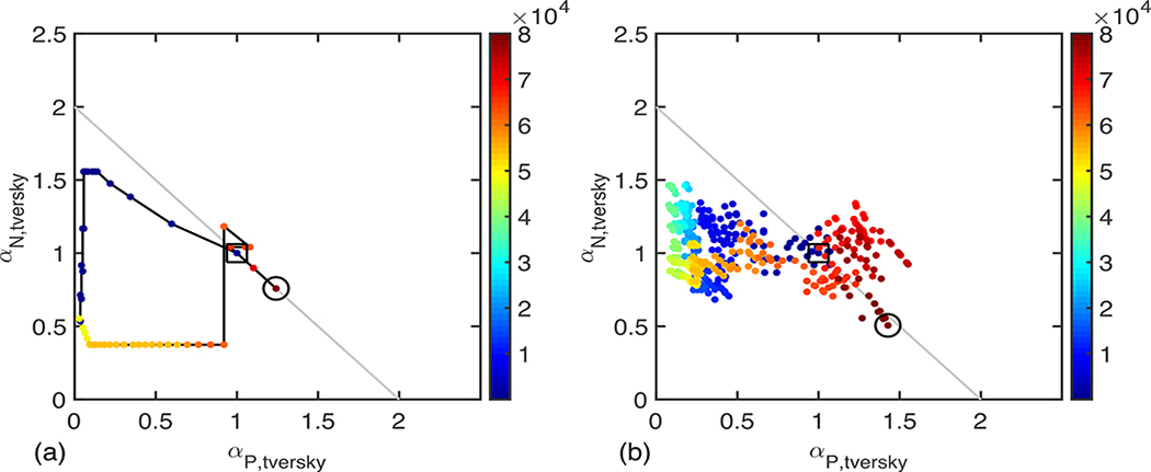
Figure 7 shows the trajectory of the GLF coefficients in a 2D space obtained by projecting the values of the coefficients along the axes α_P,tversky = 2 α_P⁄(1 + β²) and ${\alpha }_{N,\text{tversky}}=2{\beta }^2{\alpha }_P/\left(1+{\beta }^2\right)$. This step is motivated by noticing that with this change of variable, the GLF also collapses to the conventional Tversky loss function. This figure shows that in both cases, a large portion of the parameter space is explored during the training of the network, which would have remained unexplored if the coefficients had been fixed ahead of training. Figure 7 visually ratifies the intuition that at some point during training, due to poor performance of the network, it is necessary to alter the values of these coefficients, for example by significantly decreasing the false positive weighting to favor the false negative weighting, but that towards the end of training, the parameter values recover more balanced values (1.4, 0.5) and (1.2, 0.8) for the deterministic and exploratory methods, respectively.

Fig. 7.

Two-dimensional trajectory of the coefficients α_P, α_N, and β² during training mapped in the Tversky coefficients space α_P,tversky = 2 α_P/(1 + β²) and ${\alpha }_{N,\text{tversky}}=2{\beta }^2{\alpha }_P/\left(1+{\beta }^2\right)$. In this representation, using the Dice loss corresponding to operating at a fixed point (1,1), using the Effectiveness loss corresponding to operating at a fixed point on the gray line α_P,tversky + α_N,tversky = 2, and using the Tversky loss corresponding operating at a fixed point anywhere in the plane defined by α_P,tversky ≥ 0 and α_N,tversky ≥ 0. With the adaptive training methodology, the parameters are updated at every iteration step leading to a dynamic trajectory as the optimization is carried out (colormap correspond to iteration number).

IV. Discussion

A number of pitfalls exist in current deep learning modeling, which often adversely affects the performance of deep learning-based decision-making. Among them are the choice of the loss function and the way of deciding the involved hyperparameter values. These two fundamental issues have received relatively little attention despite the known intimate relationship between the choice of loss function and the outcome of model prediction. In this study, we bring up a three-dimensional parameterization of a GLF and an adaptive training scheme to close the gap between deep neural network modeling and decision-making metrics. The multi-dimensional parameterization of the loss function allows the flexible weighting of distinct metrics relevant to the final decision-making, and the adaptive evolution of the model parameters during neural network training makes it possible to maximally utilize the capacity of deep neural network.

Two intuitive algorithms are developed to meet the challenges of the new learning framework. The first one, a greedy adaptive method, relies on choosing the best parameter update following the exhaustive exploration of 3 predefined actions for each parameter at each iteration step of the optimization algorithm. And the second approach, a deterministic adaptive method, updates the parameters using a rule-based algorithm. Partly motivated by a mathematical analysis of the gradient of the loss function, this second interpretable method introduces little computational overhead and is flexible enough to be deployed into most existing deep learning frameworks. The hyperparameter of the proposed adaptive loss can, in principle, be tuned based on reinforcement learning. But this will entail a careful implementation and detailed evaluation of a computationally intensive reinforcement learning scheme. Due to the large scope of the approach, we postpone the investigation to the future.

In the context of biomedical image segmentation, the proposed formalism generalizes the conventional Dice, Effectiveness and Tversky loss functions. Additionally, the adaptive training methods allow dynamic exploration of a larger portion of the parameter space. Numerical experiments demonstrated that the detection and segmentation of lung and liver tumors are consistently improved compared to conventional training methodologies. Most remarkably, networks trained with the proposed methods are capable of discerning small tumors less than 100 pixels in size, which is less than 0.04% of the total 512² pixel dimension of an entire CT scan slice.

Deep learning networks are often criticized for their “black box” nature [33, 34], and for the difficulty to rationalize the manual tuning of the numerous hyperparameters. Similar to that of model parameters optimization in treatment planning [9, 35], the proposed methodology improves the performance of deep learning-based decision-making while concurrently providing better interpretability of the evolution of the parameters. The examples presented in this study showcased how the adaptive changes in the parameters can be intuitively related to imbalance in the training related to small regions of interest in otherwise large input data. The proposed formalism opens new opportunities for numerous other practical applications.

References

- [1].Krizhevsky A, Sutskever I, and Hinton GE, “Imagenet classification with deep convolutional neural networks.” pp. 1097–1105.
- [2].Simonyan K, and Zisserman A, “Very deep convolutional networks for large-scale image recognition,” arXiv preprint arXiv:1409.1556, 2014. [Google Scholar]
- [3].Collobert R, and Weston J, “A unified architecture for natural language processing: Deep neural networks with multitask learning.” pp. 160–167.
- [4].Gulshan V, Peng L, Coram M, Stumpe MC, Wu D, Narayanaswamy A, Venugopalan S, Widner K, Madams T, and Cuadros J, “Development and validation of a deep learning algorithm for detection of diabetic retinopathy in retinal fundus photographs,” Jama, vol. 316, no. 22, pp. 2402–2410, 2016. [DOI] [PubMed] [Google Scholar]
- [5].Esteva A, Kuprel B, Novoa RA, Ko J, Swetter SM, Blau HM, and Thrun S, “Dermatologist-level classification of skin cancer with deep neural networks,” Nature, vol. 542, no. 7639, pp. 115, 2017. [DOI] [PMC free article] [PubMed] [Google Scholar]
- [6].Ting DSW, Cheung CY-L, Lim G, Tan GSW, Quang ND, Gan A, Hamzah H, Garcia-Franco R, San Yeo IY, and Lee SY, “Development and validation of a deep learning system for diabetic retinopathy and related eye diseases using retinal images from multiethnic populations with diabetes,” Jama, vol. 318, no. 22, pp. 2211–2223, 2017. [DOI] [PMC free article] [PubMed] [Google Scholar]
- [7].Poplin R, Varadarajan AV, Blumer K, Liu Y, McConnell MV, Corrado GS, Peng L, and Webster DR, “Prediction of cardiovascular risk factors from retinal fundus photographs via deep learning,” Nature Biomedical Engineering, vol. 2, no. 3, pp. 158, 2018. [DOI] [PubMed] [Google Scholar]
- [8].Ibragimov B, Toesca D, Chang D, Yuan Y, Koong A, and Xing L, “Development of deep neural network for individualized hepatobiliary toxicity prediction after liver SBRT,” Medical physics, vol. 45, no. 10, pp. 4763–4774, 2018. [DOI] [PMC free article] [PubMed] [Google Scholar]
- [9].Xing L, Li J, Donaldson S, Le Q, and Boyer A, “Optimization of importance factors in inverse planning,” Physics in Medicine & Biology, vol. 44, no. 10, pp. 2525, 1999. [DOI] [PubMed] [Google Scholar]
- [10].Ruder S, “An overview of gradient descent optimization algorithms, ” arXiv preprint arXiv:1609.04747, 2016. [Google Scholar]
- [11].Milletari F, Navab N, and Ahmadi S-A, “V-net: Fully convolutional neural networks for volumetric medical image segmentation.” pp. 565–571.
- [12].Lguensat R, Sun M, Fablet R, Tandeo P, Mason E, and Chen G, “EddyNet: A deep neural network for pixel-wise classification of oceanic eddies.” pp. 1764–1767.
- [13].Hashemi SR, Salehi SSM, Erdogmus D, Prabhu SP, Warfield SK, and Gholipour A, “Asymmetric loss functions and deep densely-connected networks for highly-imbalanced medical image segmentation: Application to multiple sclerosis lesion detection,” IEEE Access, vol. 7, pp. 1721–1735, 2018. [DOI] [PMC free article] [PubMed] [Google Scholar]
- [14].Salehi SSM, Erdogmus D, and Gholipour A, “Tversky loss function for image segmentation using 3D fully convolutional deep networks.” pp. 379–387.
- [15].Sasaki Y, and Fellow R, “The truth of the F-measure, Manchester: MIB-School of Computer Science,” University of Manchester, 2007. [Google Scholar]
- [16].Ronneberger O, Fischer P, and Brox T, “U-Net: Convolutional Networks for Biomedical Image Segmentation,” arXiv e-prints, https://ui.adsabs.harvard.edu/abs/2015arXiv150504597R, [May 01, 2015, 2015]. [Google Scholar]
- [17].Brosch T, Yoo Y, Tang LY, Li DK, Traboulsee A, and Tam R, “Deep convolutional encoder networks for multiple sclerosis lesion segmentation.” pp. 3–11. [DOI] [PubMed]
- [18].Lin T-Y, Goyal P, Girshick R, He K, and Dollár P, “Focal loss for dense object detection.” pp. 2980–2988. [DOI] [PubMed]
- [19].Wong KC, Moradi M, Tang H, and Syeda-Mahmood T, “3d segmentation with exponential logarithmic loss for highly unbalanced object sizes.” pp. 612–619.
- [20].Abraham N, and Khan NM, “A novel focal tversky loss function with improved attention U-Net for lesion segmentation.” pp. 683–687.
- [21].Naceur MB, Kachouri R, Akil M, and Saouli R, “A New Online Class-Weighting Approach with Deep Neural Networks for Image Segmentation of Highly Unbalanced Glioblastoma Tumors.” pp. 555–567.
- [22].Nesterov Y, “A method for unconstrained convex minimization problem with the rate of convergence O (1/k^ 2).” pp. 543–547.
- [23].Bengio Y, Boulanger-Lewandowski N, and Pascanu R, “Advances in optimizing recurrent networks.” pp. 8624–8628.
- [24].Duchi J, Hazan E, and Singer Y, “Adaptive subgradient methods for online learning and stochastic optimization,” Journal of Machine Learning Research, vol. 12, no. Jul, pp. 2121–2159, 2011. [Google Scholar]
- [25].Kingma DP, and Ba J, “Adam: A method for stochastic optimization,” arXiv preprint arXiv:1412.6980, 2014. [Google Scholar]
- [26].Dozat T, “Incorporating nesterov momentum into adam.”
- [27].Recht B, Re C, Wright S, and Niu F, “Hogwild: A lock-free approach to parallelizing stochastic gradient descent.” pp. 693–701.
- [28].Zeiler MD, “ADADELTA: an adaptive learning rate method,” arXiv preprint arXiv:1212.5701, 2012. [Google Scholar]
- [29].Seo H, Huang C, Bassene M, and Xing L, “Modified U-Net (mU-Net) with Incorporation of Object-Dependent High Level Features for Improved Liver and Liver-Tumor Segmentation in CT Images,” IEEE Transactions on Medical Imaging vol. 10.1109/TMI.2019.2948320, 2019. [DOI] [PMC free article] [PubMed] [Google Scholar]
- [30].Abadi M, Barham P, Chen J, Chen Z, Davis A, Dean J, Devin M, Ghemawat S, Irving G, Isard M, Kudlur M, Levenberg J, Monga R, Moore S, Murray DG, Steiner B, Tucker P, Vasudevan V, Warden P, Wicke M, Yu Y, and Zheng X, “TensorFlow: A system for large-scale machine learning,” arXiv e-prints, https://ui.adsabs.harvard.edu/abs/2016arXiv160508695A, [May 01, 2016, 2016]. [Google Scholar]
- [31].Simpson AL, Antonelli M, Bakas S, Bilello M, Farahani K, van Ginneken B, Kopp-Schneider A, Landman BA, Litjens G, Menze B, Ronneberger O, Summers RM, Bilic P, Christ PF, Do RKG, Gollub M, Golia-Pernicka J, Heckers SH, Jarnagin WR, McHugo MK, Napel S, Vorontsov E, Maier-Hein L, and Cardoso MJ, “A large annotated medical image dataset for the development and evaluation of segmentation algorithms,” arXiv e-prints, https://ui.adsabs.harvard.edu/abs/2019arXiv190209063S, [February 01, 2019, 2019]. [Google Scholar]
- [32].Bilic P, Christ PF, Vorontsov E, Chlebus G, Chen H, Dou Q, Fu C-W, Han X, Heng P-A, Hesser J, Kadoury S, Konopczynski T, Le M, Li C, Li X, Lipkovà J, Lowengrub J, Meine H, Hendrik Moltz J, Pal C, Piraud M, Qi X, Qi J, Rempfler M, Roth K, Schenk A, Sekuboyina A, Vorontsov E, Zhou P, Hülsemeyer C, Beetz M, Ettlinger F, Gruen F, Kaissis G, Lohöfer F, Braren R, Holch J, Hofmann F, Sommer W, Heinemann V, Jacobs C, Efrain Humpire Mamani G, van Ginneken B, Chartrand G, Tang A, Drozdzal M, Ben-Cohen A, Klang E, Amitai MM, Konen E, Greenspan H, Moreau J, Hostettler A, Soler L, Vivanti R, Szeskin A, Lev-Cohain N, Sosna J, Joskowicz L, and Menze BH, “The Liver Tumor Segmentation Benchmark (LiTS),” arXiv e-prints, https://ui.adsabs.harvard.edu/abs/2019arXiv190104056B, [January 01, 2019, 2019]. [Google Scholar]
- [33].Oh SJ, Augustin M, Schiele B, and Fritz M, “Towards Reverse-Engineering Black-Box Neural Networks,” arXiv e-prints, https://ui.adsabs.harvard.edu/abs/2017arXiv171101768O, [November 01, 2017, 2017]. [Google Scholar]
- [34].Lei D, Chen X, and Zhao J, “Opening the black box of deep learning,” arXiv e-prints, https://ui.adsabs.harvard.edu/abs/2018arXiv180508355L, [May 01, 2018, 2018]. [Google Scholar]
- [35].Yang Y, and Xing L, “Inverse treatment planning with adaptively evolving voxel-dependent penalty scheme,” 10, Wiley, 2004. [DOI] [PubMed] [Google Scholar]
Associated Data
This section collects any data citations, data availability statements, or supplementary materials included in this article.