On the Robustness of Deep Learning based Lung Nodule Classification for CT Images with respect to Image Noise

Abstract

Robustness is an important aspect when evaluating a method of medical image analysis. In this study, we investigated robustness of a deep learning-based lung nodule classification model for CT images with respect to noise perturbations. A deep neural network (DNN) was established to classify 3D CT images of lung nodules into malignant or benign groups. The established DNN was able to predict malignancy rate of lung nodules based on CT images, achieving the area under the curve (AUC) of 0.91 for the testing dataset in a 10-fold cross validation as compared to radiologists’ prediction. We then evaluated its robustness against noise perturbations. We added to the input CT images noise signals generated randomly or via an optimization scheme using a realistic noise model based on a noise power spectrum for a given mAs level, and monitored the DNN’s output. The results showed that the CT noise was able to affect the prediction results of the established DNN model. With random noise perturbations at 100 mAs, DNN’s predictions for 11.2% of training data and 17.4% of testing data were successfully altered by at least once. The percentage increased to 23.4% and 34.3%, respectively, for optimization-based perturbations. We further evaluated robustness of models with different architectures, parameters, number of output labels etc., and robustness concern was found in these models to different degrees. To improve model robustness, we empirically proposed an adaptive training scheme. It fine-tuned the DNN model by including perturbations in the training dataset that successfully altered the DNN’s perturbations. The adaptive scheme was repeatedly performed to gradually improve DNN’s robustness. The numbers of perturbations at 100 mAs affecting DNN’s predictions were reduced to 10.8% for training and 21.1% for testing by the adaptive training scheme after two iterations. Our study illustrated that robustness may potentially be a concern for an exemplary deep learning-based lung nodule classification model for CT images, indicating the needs for evaluating and ensuring model robustness when developing similar models. The proposed adaptive training scheme may be able to improve model robustness.

1. INTRODUCTION

Deep learning (DL) methods (LeCun et al., 2015; Shen et al., 2020) have gained increasing interest in a wide spectrum of machine learning problems (Szegedy et al., 2013; Yu et al., 2013; Simonyan et al., 2013; Mnih et al., 2013; Mnih et al., 2015; Silver et al., 2016; Wang, 2016; Goodfellow et al., 2014; Zhu et al., 2016). One of the major groundbreakings is in natural image classification, where DL has been shown to obtain superhuman performance (Russakovsky et al., 2015; Krizhevsky et al., 2012). The success of DL has also been extended to healthcare regime. A number of studies incorporating DL for diagnosis and outcome prediction (Hua et al., 2015; Kumar et al., 2015; Sturm et al., 2016; Nie et al., 2016; Che et al., 2016; Li et al., 2016; Kallenberg et al., 2016; Cheng et al., 2016; Zhen et al., 2017) have achieved superior performance compared to traditional machine learning algorithms, comparable or even better than experienced clinicians in some applications (Rajpurkar et al., 2017; Wang et al., 2017).

The main idea of DL is to employ a deep neural network (DNN), a large-scale hierarchical model using a multi-layer architecture, to approximately represent a distribution by learning from data. A typical DNN contains a large number of linear/non-linear numerical operations to connect different layers. The complex function form allows a DNN to flexibly approximate a complex data distribution compared to traditional machine learning methods. However, the complex functions also post a technical barrier for the theoretical analysis of a DNN to fully understand its mathematical properties, such as approximation accuracy, robustness, etc. Investigating these properties is necessary to warrant a safe application of DL techniques to a broad scope of real problems with confidence.

Robustness of a DL-based prediction model refers to its ability to tolerate perturbation/noise to the network input. Recent studies in natural image processing have revealed that robustness of DL-models is a concern, as the output can be easily affected by small-scale perturbations added to the input (Yuan et al., 2019; Su et al., 2019; Akhtar and Mian, 2018; Evtimov et al., 2017; Madry et al., 2017). Given the fact that noise inevitably exists in real medical data, robustness is of particular importance for medical applications (Shen et al., 2020), since poor robustness may mislead clinical decision making and generate severe consequences to patients. For instance, the noise level in clinical diagnosis CT images is on the order of 10–60 HU depending on the specific imaging protocols for different applications (Christianson et al., 2015). For models making predictions based on CT images, it is critical to achieve a robust performance with respect to the noise in the input images. A model with poor robustness can have instable performance, potentially influencing diagnosis decision and treatment outcome.

In this paper, we studied the robustness of an example problem of DL-based lung-nodule classification for CT images. While theoretical robustness analysis remains challenging, we investigated this empirically through numerical studies. Specifically, we examined the performance of a DL-model that classifies CT images of lung nodules into benign and malignant classes by injecting noise perturbations to the input images and observing the effects on the model output. The studies revealed that robustness of this DL model may be a concern. To mitigate this issue, we also proposed a training scheme that potentially improved robustness.

2. MATERIALS AND METHODS

2.1. Network training

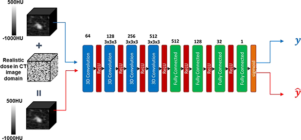
We formulated the problem of predicting benignity or malignancy of a lung nodule based on a CT image as a DNN-based binary classification problem. The structure of the DNN is depicted in Fig. 1. Input of the DNN was a 3D CT image cube containing the nodule. Four 3D convolutional layers were incorporated in the first half of the network, each followed by a rectified linear unit (ReLU) (Nair and Hinton, 2010), to extract comprehensive features from the input image. These features were then passed through four fully connected layers to perform classification. The last fully connected layer utilized a sigmoid activation function for the classification purpose. We trained the DNN by solving the following optimization problem:

$${\theta }^{*}={\mathrm{argmin}}_{\theta }{\sum }_{i\in Tr}{\Vert D\left(x_i\mid \theta \right)-y_i^{*}\Vert }_2^2,$$ (1)

where x_i ∈ R^n×n×n indicates the i-th CT image cube of size n in the training dataset Tr consisting of in total N_train training samples. $y_i^{*}\in \{0,1\}$ gives its corresponding ground truth label. $y_i^{*}=1$ if x_i is malignant and $y_i^{*}=0$ otherwise. D(·|θ*) is the DNN function with θ representing the set of network parameters to be determined through the training process. This optimization problem was solved via the widely used adaptive moment estimation method (Kingma and Ba, 2014).

Figure 1.

Structure of the deep neural network classifier in this study.

2.2. Robustness analysis

After the DNN model was trained, we evaluated its robustness against CT image noise, see Fig. 2. In this study, we focused our investigations on the impacts of noise signals under different mAs levels, one the most important parameters in CT scans. A useful prediction model should be robust against such perturbations of noise in CT. Let us denote predicted label under the original image and the image with noise added by y and $\widehat{y}$. For a robust model, $y=\widehat{y}$ should hold. On the other hand, if a model predicts inconsistent labels for the same nodule with and without adding a noise signal, the prediction is unreliable, since noise is unavoidable in real clinical settings.

Figure 2.

An example of model robustness analysis. Realistic noise in CT image domain will be added to a lung nodule CT image with a predicted label y from a DNN. The perturbed sample is also fed into the DNN, receiving a label $\widehat{y}$. The DNN is robust against the perturbation, if $y=\widehat{y}$.

In the following sections, we will investigate robustness of the deep learning-based model against noise perturbations of different mAs levels generated randomly and by an optimization method.

2.2.1. Robustness with respect to randomly sampled attacks

In this study, we considered a wide range of mAs levels, including 10, 50, 100, 200, and 500 mAs. The purpose is to perform comprehensive evaluations on the robustness of the DNN model against noise in a wide range of scanning protocols (Bhalla et al., 2019; Yanagawa et al., 2014), from the low-dose CT regime (10 and 50 mAs), to normal dose levels commonly used in clinic (100 and 200 mAs), and a high dose scenario (500 mAs).

For each mAs level, given an input CT image cube x_i, we implemented a noise power spectra (NPS) based approach (see Appendix) to generate realistic noise perturbations p_i ∈ R^n×n×n (Divel and Pelc, 2020; Dolly et al., 2016; Hsieh, 2003) with its amplitude and texture following the corresponding NPS. We repeatedly generated random perturbations for K times for each input CT cube and fed the perturbed CT cube into the DNN to compute the new output, i.e. ${\widehat{y}}_i=D\left(x_i+p_i\mid {\theta }^{*}\right)$. This was termed as attacks under the perturbation. The attack was called successful if ${\widehat{y}}_i$ is different from $y_i=D\left(x_i\mid {\theta }^{*}\right)$, the predicted label of the original CT cube x_i. A clinically desired model would predict consistent output labels, i.e. ${\widehat{y}}_i=y_i$.

2.2.2. Robustness with respect to purposely selected attacks via an optimization approach

In this step, for each input data x_i, we aimed at purposely looking for perturbations $p_i^{*}\in R^{n\times n\times n}$ following the NPS at the specified mAs level, such that the predicted label of the perturbed input was altered. This goal could be achieved by solving the following optimization problem:

$$\begin{gathered} p_i^{*}={\mathrm{argmax}}_{p_i}{\sum }_i{\Vert D\left(x_i+p_i\mid {\theta }^{*}\right)-D\left(x_i\mid {\theta }^{*}\right)\Vert }_2^2, \\ \text{s.t.}{E}_{\{\varphi ,z,i\}}\left[F\left[p_{z,i}\right](f,\varphi )\right]={\left[S(f)\frac{N_x{N}_y}{\mathrm{\Delta }x\mathrm{\Delta }y}\right]}^{1/2},p=\left\{p_1,p_2,\dots \right\}. \end{gathered}$$ (2)

Here we use p to denote the goup of all 3D noise signals generated for all samples. p_z,_i is the z axial slice of p_i. F[.] denotes the Fourier transform and f and ϕ are radial and angular coordinate in the Fourier domain. E_{ϕ,z,i}[.] represents an average operator over all angles ϕ on each 2D axial slide, all axial slices z, and all data samples. S is the NPS for the given mAs, which is a function of f because of rotational symmetry. Δx and Δy are pixel sizes, and N_x and N_y are numbers of pixels along the x and y directions. The constraint ensured the optimized perturbations on average following the noise properties specified by the NPS. Following the same setup as in the random perturbation study, we considered different NPS for 10, 50, 100, 200, and 500 mAs. We solved the optimization problem via the projected gradient ascent algorithm expressed as

$$p_i^{t-\frac{1}{2}}=p_i^{t-1}+{2\delta \left(D\left(x_i+p_i\mid {\theta }^{*}\right)-D\left(x_i\mid {\theta }^{*}\right)\right)\frac{\partial D\left(x_i+p_i\mid {\theta }^{*}\right)}{\partial p_i}|}_{p_i^{t-1}},$$ (3)

$$p^t={\mathrm{Proj}}_{\tau }\left(p^{t-\frac{1}{2}},S\right),$$ (4)

where $p^{t-\frac{1}{2}}=\{p_1^{t-\frac{1}{2}},p_2^{t-\frac{1}{2}},\dots \}$. t is the index of iteration and δ is the step size of the gradient ascend algorithm. Proj_τ(∗, S) is the projection operator to ensure the result following the NPS,

$${\mathrm{Proj}}_{\tau }\left(a_{z,i},S\right)=F^{-1}\left[\frac{F\left[a_{z,i}\right](f,\varphi )}{E_{\{\varphi ,z,i\}}\left[F\left[a_{z,i}\right](f,\varphi )\right]}{\left[S(f)\frac{N_x{N}_y}{\mathrm{\Delta }x\mathrm{\Delta }y}\right]}^{1/2}\right].$$ (5)

The iteration stopped, when $\frac{{\Vert p^t-p^{t-1}\Vert }_2}{{\Vert p^{t-1}\Vert }_2}\le ϵ$ or the maximum iteration number N_iter was reached.

Moreover, D(·|θ*) is a highly non-convex function and so is the optimization problem in Eq. (2). As such, the obtained solution varies depending on the initial solution. In this regard, for each DNN input data x_i, we repeatedly solved the problem of Eq. (2) for K times with different random initializations. The detailed algorithm is summarized in Algorithm 1.

Algorithm 1.

Generating optimization-based attack.

for i = 1, 2, …, Ntrain do

for k = 1, 2, …, K do

1. Initialize perturbation p0 randomly; set t = 0;

while t ≤ Niter do

2. Update pt following equations (3) and (4);

3. If $\frac{{\Vert p^t-p^{t-1}\Vert }_2}{{\Vert p^{t-1}\Vert }_2}\le ϵ$ or t = Niter, set $p_i^{*}(k)=p^t$, set t = Niter;

Otherwise, set t = t + 1, go to step 2;

end while

end for

end for

Output $\left\{p_i^{*}(k)\mid i=1,2,\dots ,N_{train},k=1,2,\dots ,K\right\}$

2.3. Robustness for networks with different setups

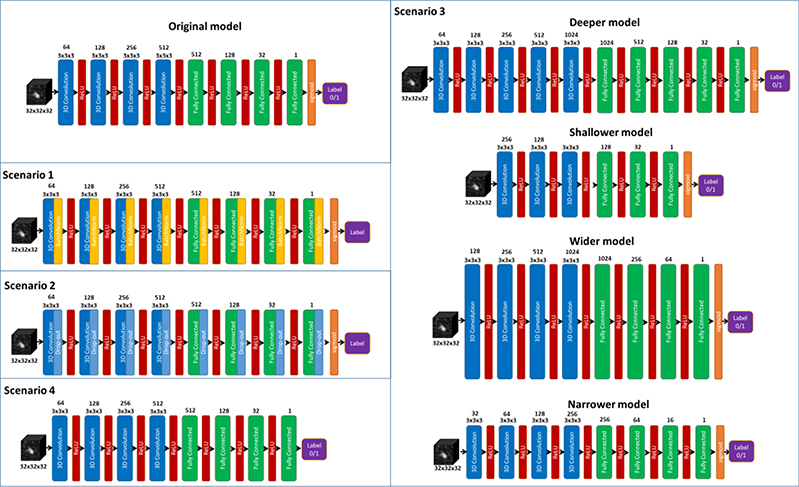
To study if the robustness is caused by the specific network setup, we also evaluated the impact of different architectures. We adjusted the architecture of the proposed DNN model to build new models for different scenarios, including 1) adding batch normalization layers, 2) adding drop-out layers of different rates (0.1 and 0.2), 3) constructing deeper, shallower, wider, narrower models, and 4) building a model to directly predict rates ranging from 1 to 5 characterizing the malignancy suspiciousness with 1 being the least suspicious and 5 indicating the most of malignancy. The detailed architecture of models built for all these scenarios are shown in Fig. 3. Specifically, for scenarios 1) and 2), batch normalization and drop-out layer were introduced, respectively, after each convolution and fully connected layers. For scenario 3), the deeper network was constructed by inserting a 3D convolution layer consisting of 1024 convolutional kernels of size 3 × 3 × 3, and a fully connected layer of size 1024 between the last convolution layer and the first fully connected layer of the original DNN, while the shallower network was formed by simply removing the these two layers. In addition, the number of neurons in each layer were increased and decreased by a factor of two, respectively, to generate the wider and narrower networks. Finally, for scenario 4), the network architecture was not modified except for removing the sigmoid function activation function to output a value from 1 to 5 representing the predicted rate of malignancy. For all these scenarios, random attack of 100 mAs was performed to evaluate the robustness.

Figure 3.

Different network architectures for a comprehensive robustness evaluation.

2.4. Visualizing attention of DNN

To have a better understanding on the DNN and its robustness, we openned the established model and visualized extracted features. More specifically, given an input sample, we first forward evaluated the DNN and saved the features computed after several typical network layers. These features are essentially the information captured by the DNN in order to determine whether a nodule is malignant or benign. Moreover, we have also generated an attention map of DNN by integrating the extracted features. It highlighted the regions in a CT image where the DNN paid the most attention to achieve the classification of lung nodules. By doing so, we could have a better understanding on how image noise changed the classification behavior of the DNN.

2.5. An empirical approach to improve robustness

We empirically propose an adaptive training scheme that could potentially improve the network’s robustness. Generally speaking, a DNN robust to perturbations should be trained via an optimization model

$${\theta }^{*}={\mathrm{argmin}}_{\theta }{\sum }_{i\in S}{\sum }_{p\in \{A,0\}}{\Vert D\left(x_i+p\mid \theta \right)-y_i^{*}\Vert }_2^2,$$ (6)

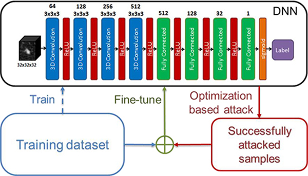
where the set A contains all the noise perturbations. Summation over p explicitly enforces the consistency between the output labels of the perturbed inputs and that of the original input. Yet enumerating all perturbations when solving the problem in Eq. (6) is impractical due to the high dimension of the input data, e.g. 32³ in the lung-nodule classification problem here. To overcome this problem, we proposed a workflow in Fig. 4 that adaptively improves robustness.

Figure 4.

Workflow of the adaptive training scheme. The dashed line indicates one-time operation to train the network initially. The solid lines show an iterative process.

More specifically, after performing the optimization-based attacks, the perturbed samples of training data that were found vulnerable were further included into an enlarged training dataset, based on which the network was finely tuned. The goal of the fine-tuning step was to improve the robustness by having the network observe those data attacking the network successfully. This process repeated, until we were satisfied with the robustness of the network. In Algorithm 2, we have summarized the detailed adaptive training scheme.

Algorithm 2.

Adaptive training scheme.

1. Train DNN for θ* by minimizing the loss function in equation (1);

for i = 1, 2, …, Nadapt do

2. Run Algorithm 1 for $\left\{p_i^{*}(k)\mid i=1,2,\dots ,N_{train},k=1,2,\dots ,K\right\}$;

3. Find a set of perturbed samples $P\subset \{x_i+p_i^{*}(k)\mid i=1,2,\dots ,N_{train},k=1,2,\dots ,K\}$ that were found vulnerable;

4. If P = ∅, set i = Nadapt;

Otherwise, Set S = S ∪ P, update θ* over enlarged S by minimizing the loss function in equation (1);

end for

Output θ*

2.6. Dataset and implementation

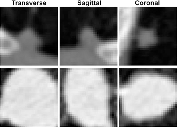
The DL-based classification network was trained using Lung Image Database Consortium (LIDC) of Image Database Resource Initiative (IDRI) (Armato et al., 2011) from The Cancer Imaging Archive (TCIA)(Clark et al., 2013). In this data set, the CT images were collected from seven academic centers and eight medical imaging companies. The dataset contains nodules of different sizes and all the nodules were rated from 1 to 5 by multiple radiologists based on their malignancy suspiciousness with 1 being the least suspicious and 5 indicating the most. In our study, we considered only those nodules with the size larger than or equal to 3 mm. For each selected nodule, the average value of all ratings given by all radiologists was utilized to indicate the level of malignancy suspiciousness. We further removed those ambiguous nodules rated at 3, yielding a set of CT images containing 1,226 nodules with 431 malignant (rating >3) and 795 benign ones (rating <3). All CT images were interpolated to a resolution of 1 mm along all three dimensions. For each nodule, a 3-D image cube of size 32×32×32 voxels was extracted from the CT image as the model input. We show in Fig. 5 three orthogonal views of image cubes extracted from two representative cases, one benign case and one malignant case.

Figure 5.

Three orthogonal views of extracted lung nodule cubes from one benign (top) and one malignant case (bottom).

Within 1263 CT cubes in our dataset, 80% (981) were randomly picked for training and validation, and the remaining (N_test=245) were saved for testing purpose. During the training process of the DNN model, a 10-fold cross validation strategy was implemented. The 981 samples selected for training was randomly split into 10 groups of approximately the same size. For the training of each fold, we picked one group as validation set (N_val = 98) while the remaining samples were used for model training (N_train =883). As an independent testing dataset, all the testing data samples were left out during the training process and hence never utilized in the 10-fold cross validation process. Performance of the model in each fold was not evaluated on the testing data until the training for the 10 folds was completed. Data augmentation was also performed to enlarge the training dataset by randomly shifting (maximally five pixels in each direction) and rotating (maximally 15 degrees about each axis) the images.

Our study was implemented using Python with TensorFlow (Abadi et al., 2016) on a desktop workstation equipped with eight Intel Xeon 3.5 GHz CPU processors, 32 GB memory and two Nvidia Quadro M4000 GPU cards. We trained the network with 500 epochs with a batch size of 64 and a learning rate of 1 × 10⁻⁵. To address the imbalanced malignant (345) and benign (636) samples in the training set, we adjusted sampling rates to make them contribute evenly in the training process. The model with the best validation performance for each of the 10 folds was selected for the subsequent robustness analysis.

In the robustness study, for both the random attacks and the optimization-based attacks, the number of attacks K for each sample was 50. When solving the optimization problem in Eq. (2), the step size δ of the gradient ascend algorithm was 1. The gradient of the DNN with respect to p_i, i.e. $\frac{\partial D\left(x_i+p_i\mid {\theta }^{*}\right)}{\partial p_i}$, needs to be evaluated at each iteration, which was achieved using TensorFlow backend function library. The stopping criteria was ∊ = 10⁻³ and N_iter = 10. In each iteration of the adaptive training process, we performed the optimization-based attack only once for each training sample and included the successfully attacked samples in the training dataset to finely tune the network. We still chose to repeatedly attack the tuned network for K = 50 times to evaluate robustness and hence effectiveness of the adaptive training scheme. The number of epochs used for network fine-tuning at each adaptive training step was 10.

2.7. Evaluation studies

To evaluate classification performance of the network, receiver operating characteristic (ROC) curves (Green and Swets, 1966) were plotted and area under curve (AUC) was used as the metric. In addition, we also used accuracy, sensitivity, and specificity to assess performance of the binary classifier from different aspects. Specifically, accuracy, sensitivity, and specificity are defined as follows:

$$\begin{gathered} accuracy=\frac{TP+TN}{TP+TN+FP+FN}, \\ sensitivity=\frac{TP}{TP+FN}, \\ specificity=\frac{TN}{TN+FP}, \end{gathered}$$ (7)

where TP, FP, TN, and FN are numbers of true positive cases, false positive cases, true negative cases, and false negative cases, respectively.

As for the evaluation of robustness, we first defined that a sample is called successfully attacked, if its label predicted from the deep learning model is altered after applying the perturbation. Then we considered two metrics to quantify DNN’s robustness in different angles. The first one was successfully attacked samples number (SAN). SAN was simply the number of samples that were successfully attacked by at least once among the K attempts. It quantified the robustness of the DNN as evaluated on the dataset. Second, among all the samples that were successfully attacked, some were more vulnerable than others. Hence, we computed successful attack rate (SAR) for the i-th sample as

$$SAR=\frac{n_{\mathit{\text{succ}}}^i}{K}(\%)$$ (8)

to measure its vulnerability, with $n_{\mathit{\text{succ}}}^i\le K$ being the number of successful attacks for the i-th sample. A higher SAR indicated a higher vulnerability. We plotted the curve of percentage of samples that have SAR exceeding certain levels. Although the DNN was trained using the training dataset, we evaluated robustness on both the training and the testing datasets.

During the iterative adaptive training process to improve robustness, we monitored robustness of the network with the aforementioned metrics. Since prediction performance is of top priority for model development, we also monitored AUC during this process. The adaptive training process was performed using only the training dataset. However, we also evaluated robustness on the testing dataset in this process to observe generalizability of the trained model in terms of robustness. Note that successfully attacked testing samples were never involved in the adaptive training process.

3. RESULTS

3.1. Classification performance

The AUC, accuracy, sensitivity, and specificity of the proposed method on training, validation and testing dataset in the 10-fold cross validation process are reported in Table 1 (average ± standard deviation). The standard deviation was computed using results in different folds. Note that accuracy, sensitivity and specificity were computed based on a threshold value of 0.5, as it generally gave acceptable classification performance. We fixed this value for the rest of this paper. To benchmark, we compared the performance evaluated on the testing dataset with that of Multi-crop Net (Shen et al., 2017), a recently developed DL-based lung nodule classification model, which has been demonstrated to outperform the-state-of-the-art methods. Our network achieved a comparable performance to the Multi-crop Net. These classification results validated the proposed model as an effective deep learning-based model for lung nodule classification. Net. We would like to emphasize that it is not our focus to develop a new DNN architecture for lung nodule classification to outperform state-of-the-art methods. Instead, we focus on the robustness issue of this DNN model built with a representative structure for classification problems and trained to achieve a reasonable performance.

Table 1.

Classification performance on training, validation, and testing datasets (values in bold font indicate better testing performance).

Dataset	Model	AUC	Accuracy	Sensitivity	Specificity
Training	Our model	0.97±0.004	0.97±0.004	0.98±0.005	0.94±0.008
Validation	Our model	0.87±0.084	0.84±0.059	0.88±0.062	0.82±0.098
Testing	Our model	0.91±0.008	0.85±0.011	0.90±0.007	0.77±0.024
	Multi-crop Net	0.89	0.83	0.81	0.83

3.2. Robustness evaluation

We first report in Table 2 SANs under random and optimized perturbations for all the 10 DNN models generated in the 10-fold cross validation. Averaging over the 10 models, there were 439, 219.4, 98.7, 26.1, and 7.5 training samples (49.7%, 24.8%, 11.2%, 3.0% and 0.9%) were successfully attacked by at least once for 10, 50, 100, 200, and 500 mAs, respectively under random perturbations. When it came to optimization-based attacks, there were 523.7, 306.8, 206.4, 120, and 58.2 samples (59.2%, 34.7%, 23.4%, 13.6%, and 6.6%) attacked successfully. As for the testing dataset, on average over the 10 models, 128.1, 71.4, 42.6, 23.6, and 11.1 samples (52.3%, 29.1%, 17.4%, 9.6% and 4.5%) were successfully attacked by at least once for 10, 50, 100, 200, and 500 mAs, respectively, while the optimization-based attack successfully altered the predicted label of 151.1, 108.7, 84.1, 62.2, 47.3 testing samples (61.8%, 44.4%, 34.3%, 25.4%, and 19.3%).

Table 2.

Average and standard deviation of percentage of successfully attacked samples computed over 10 models generated in the 10-fold cross validation.

		SAN/Ntrain ± std (%)
		10 mAs	50 mAs	100 mAs	200 mAs	500 mAs
Random attacks	Training	49.7±4.9	24.8±4.2	11.2±4.1	3.0±2.1	0.9±0.4
	Testing	52.3±2.9	29.1±5.0	17.4±4.3	9.6±2.7	4.5±1.3
Optimized attacks	Training	59.2±6.3	34.7±6.3	23.4±6.6	13.6±6.5	6.6±4.2
	Testing	61.8±5.5	44.4±6.3	34.3±7.5	25.4±6.4	19.3±5.1

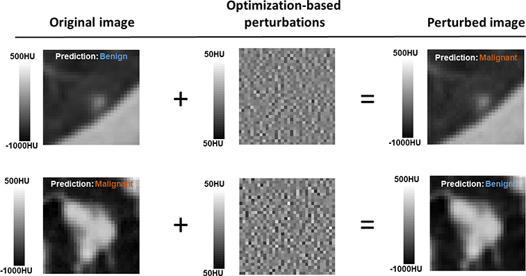
We visually inspected the images of successful attacks to confirm that they were noise-like and did not contain spatial structures that may add features to the input CT image. Examples of successfully attacked CT images and their corresponding perturbations with 500 mAs are shown in Fig. 6. As the noise amplitude was small, the perturbed and the original images were visually indistinguishable in a standard display window, and hence were expected to generate the same prediction results. However, the outputs from the network were different.

Figure 6.

By adding the optimization-based perturbations with 500 mAs, the perturbed images were misclassified.

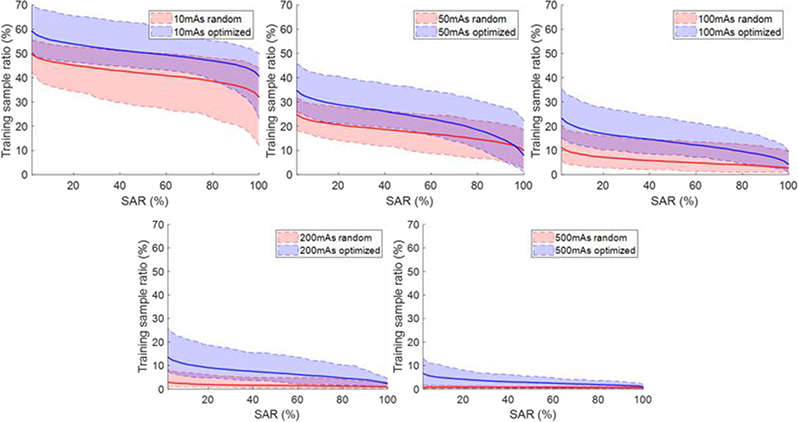
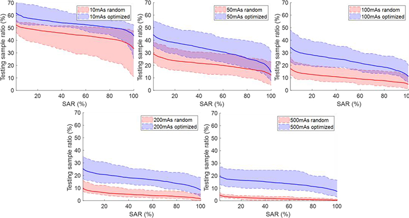
Figure. 7 and 8 plot the percentage of samples with SAR exceeding certain levels under random and optimized attacks for training and testing datasets, respectively. In general, the curves were higher for lower mAs levels, since the amplitude of noise increases when reducing the mAs level. The curves for the optimization-based perturbations were consistently higher than those for the random perturbations, because the optimization-based approach tried to deliberately attack the network.

Figure 7.

Percentage of samples with successful attack rate (SAR) exceeding certain levels on training data. Shaded region around each curve shows range computed over the 10 models.

Figure 8.

Percentage of samples with successful attack rate (SAR) exceeding certain levels on testing data. Shaded region around each curve shows range computed over the 10 models.

3.3. Robustness of networks with different architectures

Table 3 reports the robustness evaluated for networks of different architectures trained for different scenarios under random attacks at 100 mAs level as an example. The results revealed that batch normalization and drop-out layers, which are commonly used layers incorporated to regularize model training, did not help much to improve the network robustness. In addition, we evaluated robustness of networks with different model sizes. It is well known that the networks of larger sizes, e.g. deeper/wider networks, are expected to fit the training data more accurately compared to the original network due to their larger network capacities, while smaller networks, e.g. shallower/narrower networks, are less capable in data fitting. In contrast, the impact of model size to network robustness is still unclear in the deep learning regime. According to our numerical experiments, adding/removing layers and neurons did affect the model robustness. The network robustness was slightly degraded for the deeper and narrower networks, while it was improved a little for shallower and wider networks. Overall speaking, the robustness of all these models was still on the similar level. The impact of reformulating the binary classification into malignance rate prediction seemed to have the largest influence on the model robustness among all the adjustments, substantially deteriorating the model robustness. Compared to the original binary classification problem, the complexity of the new task was increased substantially while the amount of training data available remains unchanged. Giving the limited number of available training samples, it is a particularly challenging problem to figure out accurate and robust way to differentiate samples especially for those receiving close rates, for instance, to distinguish nodules rated as 1 from those rated as 2. Hence, it is expected that the resulting network is not as robust as the one established for binary classification, while even a small perturbation may have a large chance to affect the labeling process of the established model.

Table 3.

Percentage of samples attacked successfully at 100 mAs level for different network architectures.

			SAN/Ntrain (%)
			Training	Testing
100 mAs Random attacks		Original	11.2±4.1	17.4±4.3
	Scenario 1	Batch-Norm	10.6±3.7	15.7±4.4
	Scenario 2	Drop-out (0.1)	13.4±4.8	27.4±5.1
		Drop-out (0.2)	10.2±4.0	20.0±4.5
	Scenario 3	Deeper	12.0±5.2	23.2±5.6
		Shallower	9.1±3.7	17.9±4.2
		Wider	9.6±3.9	15.8±3.6
		Narrower	12.7±4.7	28.5±4.6
	Scenario 4	Five-class	26.2±6.9	86.5±15.3

3.4. Attention of DNN

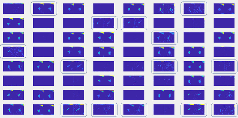
The DNN in Fig. 1 can be generally divided into two parts for feature extraction (Layers 1–4) and for decision making (Layers 5–8) based on extracted features. We fed into the DNN a CT cube with and without noise, and visualize the values processed by the network after the first layer, namely the information at the upstream of convolutional layers for feature extraction. We chose a case, such that the added noise signal was able to alter the network output. The result is shown in Fig. 9. There are 64 groups of images, corresponding central axial slices of the 64 extracted features. In each group, the left image is the one for the CT cube without noise, whereas the right one corresponds to the CT with noise added. It was observed that there are some features that are very sensitive to noise and hence the feature images were changed dramatically by the input noise, such as those highlighted by the boxes. Hence, it seems the trained network contained some feature extraction components that are relatively sensitive to the input noise.

Figure 9.

Comparison of information at position 1 between input CT with and without noise added.

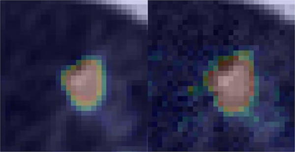
Moreover, we generated an attention map for this case, see Fig. 10. The colored regions highlighted in the images indicate the regions where the established DNN paid attention to. As we can see, the DNN focused on a larger area beyond the nodule on the attacked image while the region of importance matches with nodule quite well on the original training sample.

Figure 10.

Attention map for a nodule without noise added (left) and with noise that successfully attacked the network (right). The maps are overlaid on CT images.

3.5. Adaptive training to improve robustness

Robustness, as quantified by SAN/N_train (%), as well as AUC evaluated on the training dataset during the adaptive training process are summarized in Table 4. By including perturbed samples that successfully attacked the trained network in the training dataset, model robustness was improved. We also observed that the model AUC also gradually increased in this process. This could be ascribed to the fact that adding the optimization-based perturbations may also serve as a data augmentation scheme.

Table 4.

DNN AUC and robustness evaluated on training dataset during adaptive training. Average and standard deviations are computed over the 10 models.

	AUC±std	SAN/Ntrain ± std (%)
		10 mAs	50 mAs	100 mAs	200 mAs	500 mAs
w/o adaptive training	0.97±0.004	59.2±6.3	34.7±6.3	23.4±6.6	13.6±6.5	6.6±4.2
1 step adaptive training	0.98±0.003	37.0±6.7	20.3±2.2	15.2±2.5	10.4±2.4	6.4±1.4
2 steps adaptive training	0.99±0.008	33.5±7.6	17.4±2.2	10.8±1.7	7.7±1.8	4.7±1.2

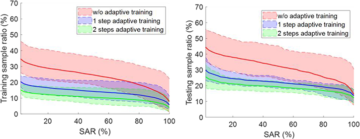
When evaluating the adaptively trained network on testing data, we surprisingly found that the robustness was also improved and so was the AUC, as shown in Table 5. Fig. 11 depicts how the percentage of samples with SAR exceeding certain levels evolved along the adaptive training steps. As attacks at different mAs levels share the similar behavior, we only show the curves for the 50 mAs case with optimization-based attacks on both training and testing datasets. In both scenarios, the ratio of successfully attacked training samples was consistently reduced. For the testing dataset, applying the adaptive training scheme once was able to improve the model robustness. Repeating the scheme for more time seemed to further improve robustness, but the improvement was small.

Table 5.

DNN AUC and robustness evaluated on testing dataset during adaptive training. Average and standard deviations are computed over the 10 models.

	AUC±std	SAN/Ntrain ± std (%)
		10 mAs	50 mAs	100 mAs	200 mAs	500 mAs
w/o adaptive training	0.91±0.008	61.8±5.5	44.4±6.3	34.3±7.5	25.4±6.4	19.3±5.1
1 step adaptive training	0.90±0.011	39.9± 11.6	29.8±6.3	27.8±7.5	20.7±6.5	16.5±6.7
2 steps adaptive training	0.90±0.013	33.9±8.5	25.6±5.2	21.1±2.6	12.4±5.8	16.1±5.3

Figure 11.

Evolution of percentage of samples with successful attack rate (SAR) exceeding certain levels during the adaptive training process. Shaded region around each curve shows range computed over the 10 models.

4. CONCLUSION AND DISCUSSIONS

In this study, we illustrated that robustness may potentially be a concern for a DL-based lung nodule classification model for CT images. Following a standard strategy to train the classification model, the established network was able to classify nodules accurately, but the prediction may be vulnerable against noise in CT images. At 100mAs level, on average 11.2% and 23.4% of training dataset and 17.4% and 34.3% of testing dataset were successfully attacked by random and optimization-based attacks in our 10-fold cross validations. To mitigate this issue, we employed an empirical scheme that included those vulnerable training samples to fine tune the model. After two iterations, rate of successful attacks reduced to 10.8% for the optimization-based attacks in the training dataset and to 21.1% in the testing set.

Using a representative example problem of DL-based lung nodule classification, we illustrated the potential concern of robustness. The observed vulnerability may degrade practical values of the DL model in real clinical applications, as noise signals are inevitable in a real clinical context, and model performance under noise perturbations should be stable to warrant a safe clinical implementation. We hope our study could shed some lights to this robustness issue. When developing a new model for medical applications, robustness evaluation is an important aspect and should be examined.

The optimization-based attack was analogous to adversarial attack (Yuan et al., 2019; Su et al., 2019; Akhtar and Mian, 2018; Evtimov et al., 2017; Madry et al., 2017), which has already been studied extensively for DL-based models in the context of natural image classification. In this work, we specifically target on medical image analysis, where the demand for robustness is high because of potential impacts on patient care. We also employed a relatively realistic noise model specific to the CT context.

Training, testing, and robustness evaluation of DNN models in the proposed study were performed using LIDC dataset from TCIA. This dataset consists of CT images of lung nodules with different dimensions and malignancy rates. The CT images were acquired on a number of scanners from seven academic centers and eight medical imaging companies under a variety of imaging protocols. Hence, the diversity in dataset with respect to CT scanners and protocols is expected, which is strongly desired especially when building models to solve real-world problems.

Generalizability is a central topic in machine learning (Michie et al., 1994), including DL (LeCun et al., 2015; Zhang et al., 2016). It refers to the fact that model performance observed in the training dataset can be extended to testing dataset that were not seen in the training process. In our study, robustness, as well as robustness improvement through the adaptive training process, were both found to be generalizable from training to testing. Yet, these facts were concluded based on empirical studies and theoretical reasons are still missing.

The current study has several limitations. First, as an initial study to investigate the robustness issue, we specifically focused on a typical DNN with a structure commonly used for classification and trained following standard settings using a dataset with a modest size. Although we have studied a variety of different network setups, such as adding batch normalization and drop-out layers, adding/removing layers, increasing/decreasing neurons in each layer, and formulating the problem directly as nodule malignancy prediction other than binary classification, the conclusion drawn here may be still limited only to the setups investigated in this study. Comprehensive evaluations of robustness on a wide range of different applications with different types of network architectures are necessary and will be our future study. Second, although a mixed dataset acquired from different institutions was employed in the proposed study, the impact of vendor/scanner and imaging protocol was not investigated. To systematically evaluate their influences to the robustness of a DNN, a number of comprehensive datasets need to be collected on scanners from different vendors under a variety of imaging protocols. It is our future work to collect such datasets and perform dedicated in-depths investigations on their impacts to DNN robustness. Third, the study only revealed the robustness issue for a DNN model, but the reason causing the problem is still unclear. Our preliminary finding (e.g. Fig. 9 and 10) indicates that some features extracted by the DNN were sensitive to the noise in the input. While this fact may account for the observed robustness problem, subsequent studies are necessary to confirm it and to have a complete understanding about it. Fourth, one drawback of the noise generation approach was that it ignored the spatial variance of NPS in a CT image. It is known that CT noise is not stationary, and NPS depends on the CT cube location. We ignored the position information, because the input to the DNN was a CT image cube containing a lung nodule, rather than an entire CT image. Hence, the generated noise can be considered as following the average behavior of noise statistics in a CT image. It is our ongoing study to perform experimental evaluations on this robustness issue in a CT-based classification task using phantoms, which will overcome this drawback in the current study. Fifth, although they have been employed as reference in many previous studies (Lei et al., 2020; Li et al., 2019; Xie et al., 2019; Al-Shabi et al., 2019; Liao et al., 2019; Shen et al., 2017; Ren et al., 2020), the labels of the nodules used in this study are given by radiologists, not based on pathological assessments. Therefore, validity of the labels may not be guaranteed. However, the major goal of this work is to evaluate how vulnerable a trained neural network is to noise perturbations in the CT images, but not the classification performance of the neural network. For this purpose, we expect that it is unlikely for the issue in data labeling to affect the validity of the robustness analysis, as long as a reasonably accurate model was studied. Of course, to develop a model that can be applied in real clinic, training using pathologically confirmed data as reference is necessary to ensure the prediction validity, which is beyond the scope of this study.

APPENDIX. ADDING NOISE TO CT IMAGES

It is well known that CT image noise is not stationary. Hence, we employed the concept of local Noise Power Spectrum (NPS) to describe noise statistics in a 2D axial image patch (Riederer et al., 1978). The NPS S(k_x, k_y) is defined as

$$S\left(f_x,f_y\right)=\frac{\mathrm{\Delta }x\mathrm{\Delta }y}{N_x{N}_y}\langle F{[p(x,y)]}^2\rangle ,$$ (A.1)

where f_x, f_y are frequencies in the Fourier space, Δx and Δy are pixel sizes, and N_x and N_y are numbers of pixels along the x and y directions. p(x, y) is the noise signal. F[.] denotes the Fourier transform, and 〈.〉 is ensemble average. To generate a noise signal for a patch, we first took the known form of the NPS corresponding to a reference setup of 120 kVp and 250 mAs as described in (Dolly et al., 2016) and linearly scaled the NPS amplitude based on the specific mAs level in our study. We then generated an image in the Fourier space with uncorrelated standard Gaussian white noise I(f_x, f_y). Finally, the noise image was computed as

$$p(x,y)=F^{-1}\left[{\left[S\left(f_x,f_y\right)\frac{N_x{N}_y}{\mathrm{\Delta }x\mathrm{\Delta }y}\right]}^{\frac{1}{2}}I\left(f_x,f_y\right)\right],$$ (A.2)

where F⁻¹ denotes inverse Fourier transform.

We demonstrate the validity of this approach by repeatedly generating 1000 noisy signals for a given NPS and estimating the NPS using Eq. (A.1). The results are shown in Fig. A1. The noise image shows a certain texture and the estimated NPS matched well with the given NPS.

Figure A1.

(a) The given NPS. (b) One example of generated noise images. (c) Estimated NPS. (d) Comparison between the given NPS (curve) and estimated NPS (dots) plotted along a radial line.

For the 3D CT image cube used in this study, a noise signal in each axial slice was generated independently following the algorithm described above.

As the CT noise is nonstationary, the noise variance and NPS of a CT image patch in fact depend on the position of the patch in the entire CT image. Hence, one apparent drawback of the above algorithm approach is that it ignored the position-dependent noise statistics. The generated noise can be considered as following the average behavior of noise statistics in a CT image.