

Abstract
One of the most prevalent joint disorders in the United States, osteoarthritis (OA) is characterized by progressive degeneration of articular cartilage, primarily in the hip and knee joints, which results in significant impacts on patient mobility and quality of life. To date, there are no existing curative therapies for OA able to slow down or inhibit cartilage degeneration. Presently, there is an extensive body of ongoing research to understand OA pathology and discover novel therapeutic approaches or agents that can efficiently slow down, stop, or even reverse OA. Thus, it is crucial to have a quantitative and reproducible approach to accurately evaluate OA-associated pathological changes in the joint cartilage, synovium, and subchondral bone. Currently, OA severity and progression are primarily assessed using the Osteoarthritis Research Society International (OARSI) or Mankin scoring systems. In spite of the importance of these scoring systems, they are semiquantitative and can be influenced by user subjectivity. More importantly, they fail to accurately evaluate subtle, yet important, changes in the cartilage during the early disease states or early treatment phases. The protocol we describe here uses a computerized and semiautomated histomorphometric software system to establish a standardized, rigorous, and reproducible quantitative methodology for the evaluation of joint changes in OA. This protocol presents a powerful addition to the existing systems and allows for more efficient detection of pathological changes in the joint.
Keywords: Medicine, Issue 159, osteoarthritis, DMM, destabilization of medial meniscus, cartilage degeneration, joint pathology, quantitative evaluation, histomorphometry
Introduction
One of the most prevalent joint disorders in the United States, OA is characterized by progressive degeneration of articular cartilage, primarily in the hip and knee joints, which results in significant impacts on patient mobility and quality of life1,2,3. Articular cartilage is the specialized connective tissue of diarthrodial joints designed to minimize friction, facilitate movement, and endure joint compression4. Articular cartilage is composed of two primary components: chondrocytes and extracellular matrix. Chondrocytes are specialized, metabolically active cells that play a primary role in the development, maintenance, and repair of the extracellular matrix4. Chondrocyte hypertrophy (CH) is one of the principal pathological signs of OA development. It is characterized by increased cellular size, decreased proteoglycan production, and increased production of cartilage matrix-degrading enzymes that eventually lead to cartilage degeneration5,6,7. Further, pathological changes in the subchondral bone and synovium of the joint play an important role in OA development and progression8,9,10,11,12. To date, there are no existing curative therapies that inhibit cartilage degeneration1,2,3,13,14. Thus, there is extensive ongoing research that aims to understand OA pathology and discover novel therapeutic approaches that are able to slow down or even stop OA. Accordingly, there is an increasing need for a quantitative and reproducible approach that enables accurate evaluation of OA-associated pathological changes in the cartilage, synovium, and subchondral bone of the joint.
Currently, OA severity and progression are primarily assessed using the OARSI or Mankin scoring systems15. However, these scoring systems are only semiquantitative and can be influenced by user subjectivity. More importantly, they fail to accurately evaluate subtle changes that occur in the joint during disease or in response to genetic manipulation or a therapeutic intervention. There are sporadic reports in the literature describing histomorphometric analyses of the cartilage, synovium, or subchondral bone16,17,18,19,20,21. However, a detailed protocol for rigorous and reproducible histomorphometric analysis of all these joint components is still lacking, creating an unmet need in the field.
To study pathological changes in OA using histomorphometric analysis, we used a surgical OA mouse model to induce OA via destabilization of the medial meniscus (DMM). Among the established models of murine OA, DMM was selected for our study because it involves a less traumatic mechanism of injury22,23,24,25,26. In comparison to meniscal-ligamentous injury (MLI) or anterior cruciate ligament injury (ACLI) surgeries, DMM promotes a more gradual progression of OA, similar to OA development in humans22,24,25,26. Mice were euthanized twelve weeks after DMM surgery to evaluate changes in the articular cartilage, subchondral bone, and synovium.
The goal of this protocol is to establish a standardized, rigorous, and quantitative approach to evaluate joint changes that accompany OA.
Protocol
Twelve-week-old male C57BL/6 mice were purchased from Jax Labs. All mice were housed in groups of 3–5 mice per micro-isolator cage in a room with a 12 h light/dark schedule. All animal procedures were performed according to the National Institute of Health (NIH) Guide for the Care and Use of Laboratory Animals and approved by the Animal Care and Use Committee of Pennsylvania State University.
1. Post-traumatic osteoarthritis (PTOA) surgical model
Anesthetize mice using a ketamine (100 mg/kg)/xylazine (10 mg/kg) combination via intraperitoneal injection, administer buprenorphine (1 mg/kg) via intraperitoneal injection for pain relief, and shave the hair over the knee. Check for the lack of a pedal reflex before starting the surgery.
-
Perform destabilization of the medial meniscus (DMM) surgery as previously described22,23.
NOTE: Please refer to Glasson et al. and Singh et al. references for more detailed surgical protocol information 22,23.
Make a 3 mm longitudinal incision from the distal patella to the proximal tibial plateau of the right knee joint. Use a suture to displace the patellar tendon.
Open the joint capsule medial to the tendon and move the infrapatellar fat pad to visualize the intercondylar region, medial meniscus, and meniscotibial ligament23.
Transect the medial meniscotibial ligament to complete DMM and destabilize the joint22,23. Close the incision site with staples or sutures.
-
Perform sham surgeries following a similar procedure, but without transection of the medial meniscotibial ligament.
NOTE: Mice were randomized to receive either DMM or sham surgery. According to the previously published literature, mice develop significant PTOA 12 weeks after the DMM surgery22,23,24.
2. Mouse euthanasia and sample collection
-
Mouse euthanasia
Twelve weeks after DMM, anesthetize mice using a ketamine (100 mg/kg)/xylazine (10 mg/kg) combination via intraperitoneal injection.
-
Make a midline incision through the skin along the thorax and retract the rib cage to expose the heart for perfusion fixation27.
NOTE: Refer to the Gage et al. reference for additional information on the protocol for proper rodent fixation as well as the video depiction of the proper equipment assembly and procedures27.
Set up the perfusion apparatus according to the manufacturer’s protocol.
-
Euthanize the mouse by perfusing heparinized saline through the left ventricle until blood is cleared out and the liver becomes pale. Perfuse the mouse with 10% neutral buffered formalin until complete mouse fixation is achieved.
NOTE: A successfully perfused mouse will become stiff. The average perfusion time using the automated pump system is 5–7 min.
-
Sample collection and preparation
Isolate the knees by cutting the bone at mid-femur and mid-tibia and dissect the surrounding muscle tissue.
Continue the fixation by storing knee joints in 10% neutral buffered formalin at room temperature for 24 h, then at 4 °C for 6 days.
-
Decalcify the bone by storing the sample in EDTA decalcification buffer for 1 week at room temperature with mild shaking28. Change the decalcification buffer solution every 3 days.
NOTE: Decalcification buffer was prepared by dissolving 140 g of ultrapure EDTA tetrasodium in a solution of 850 mL of distilled water plus 15 mL of glacial acetic acid. The buffer was pH equilibrated to 7.6 by dropwise addition of glacial acetic acid to the solution. Upon reaching pH = 7.6, the buffer was brought to 1 L total volume with distilled water. Decalcification buffer was prepared fresh and used within 1 week of preparation.
-
Wash the knees with 50% ethanol, then 70% ethanol for 15 min each, then process for embedding.
NOTE: Fluid transfer processing was performed by the Molecular and Histopathology Core at Penn State Milton S. Hershey Medical Center. Consult the institution’s histology core for recommendations on optimal sample processing.
Embed the mouse knees in paraffin with the medial aspect of the joint facing the bottom surface of the paraffin block. Apply slight pressure to the tibial side of the joint during embedding to ensure tibial and femoral surfaces are as close to the same plane as possible.
3. Microtome sectioning and slide selection
-
Microtome sectioning
Use the plane adjustment knobs on the block holder of the microtome to ensure proper facing of the sample block.
Face the paraffin block so that the distal aspect of the femur, proximal region of the tibia, and anterior and posterior horns of the medial meniscus appear in the same plane for section collection (Supplementary Figure 1A). Begin collecting sections on slides when the anterior and posterior horns of the medial meniscus begin to separate from one another.
Ensure that the tibia, femur, and menisci appear in same plane by comparing structure sizes. The tibia and femur should be of comparable size, with both meniscal horns similar in size and shape (Supplementary Figure 1A). If a structure appears too large in comparison to its counterpart, this indicates that additional facing is needed. Importantly, confirm that the joint space remains intact.
Take sagittal sections of the paraffin-embedded mouse knees through the medial joint compartment in 5 μm sections and collect the sections on slides. Collect approximately 30 sections per paraffin block.
-
Slide selection
-
Select three representative sections 50 μm apart for each sample starting from the fifth section (i.e., slides 5, 15, and 25). Selected slides will be used for subsequent staining, OARSI scoring, and histomorphometric analysis.
NOTE: From a block with 30 total sections, select slides from the beginning (slides 5–10), middle (slides 15–20), and end (slides 25–30) of the set in order to clearly represent the entire sample. Select slides from similar levels of depth between samples.
-
4. Hematoxylin, Safranin Orange, and Fast Green staining
Deparaffinize the selected slides with three changes of xylene. Hydrate the slides with two changes of 100% ethanol, two changes of 95% ethanol, and one change of 70% ethanol.
Stain the slides with hematoxylin for 7 min then wash with running water for 10 min. Stain with Fast Green for 3 min and rinse in 1.0% glacial acetic acid for 10 s. Stain with Safranin-O for 5 min and quickly rinse by dipping in 0.5% glacial acetic acid.
Rinse slides in two changes of distilled water and let air dry.
-
Clear slides in three changes of xylene for 5 min each then mount with xylene-based mounting media and a coverslip.
NOTE: Hematoxylin serves as the nuclear stain for identifying areas of bone marrow. Safranin-O is used to stain cartilage, proteoglycans, mucin, and mast cell granules. Fast Green is used as a counterstain for bone.
5. Slide imaging
Image the Safranin-O and Fast Green stained slides using an available camera attached to a microscope and computer-based imaging software.
Open the imaging software (see Table of Materials) and arrange the knee joint region of interest (ROI) in the center of the imaging window. If using a rotational microscope slide stage, align the slide so that the tibial surface spans the width of the horizontal axis of the imaging region.
-
Set the white balance of the camera before beginning to image a set of samples (Supplementary Figure 2). Image the joint compartment at both 4× and 10× magnification, ensuring that both the tibial and femoral articular surface and tibial subchondral bone are included within each of the image ROIs (Supplementary Figure 1A, B). Save images for each of the three selected levels to be used for OARSI scoring.
NOTE: Setting the white balance of the camera will depend on the software and camera systems being used. Generally, navigate to the Camera Tab or Main Imaging Menu and scroll down to Set White Balance. Select Set White Balance and a small cursor or icon should appear (Supplementary Figure 2A). Using the cursor, select an area within the image/sample that is free of stain, such as the joint space, to set the white balance.
Table of materials
| Name of Material/Equipment | Company | Catalog Number | Comments/Description |
|---|---|---|---|
| Perfusion Two Automated Pressure Perfusion system | Leica | Model # 39471005 | Sample harvest |
| 10% Buffered Formalin Phosphate | Fisher Chemical | SF100-20 | Sample fixation following harvest |
| Ethylenediaminetetraacetic acid, tetrasodium salt dihydrate, 99% | Acros Organics | AC446080010 | Decalcification Buffer preparation |
| Histosette II Tissue Cassettes - Combination Lid and Base | Fisher | 15-182-701A | Sample processing and embedding |
| Manual Rotary Microtome | Leica | RM 2235 | Sample sectioning |
| Fisherbrand Superfrost Plus Microscope Slides | Fisher | 12-550-15 | Sample section collection |
| Safranin-O stain | SIGMA Life Sciences | S8884 | Sample staining |
| Fast Green stain | SIGMA Life Sciences | F7258 | Sample staining |
| Weigerts Iron Hematoxylin A | Fisher | 5029713 | Hematoxylin staining |
| Weigerts Iron Hematoxylin B | Fisher | 5029714 | Hematoxylin staining |
| OLYMPUS BX53 Microscope | OLYMPUS | https://www.olympus-lifescience.com/en/microscopes/upright/bx53f2/https://www.olympus-lifescience.com/en/microscopes/upright/bx53f2/ | Histomorphometric analysis and imaging |
| OLYMPUS DP 73 Microscope Camera | OLYMPUS | https://www.olympus-lifescience.com/en/camera/color/dp73/ | Histomorphometric analysis and imaging (discontinued) |
| ThinkBone Stage - Rotating Stage | OsteoMetrics | http://thinkboneconsulting.com/index_files/Slideholder.php | Histomorphometric analysis and imaging |
| Cintiq 27QHD Creative Pen Display | Wacom | https://www.wacom.com/en-es/products/pen-displays/cintiq-27-qhd-touch | Histomorphometric analysis and imaging |
| Wacom Pro Pen Stylus | Wacom | https://www.wacom.com/en-es/products/pen-displays/cintiq-27-qhd-touch | Histomorphometric analysis and imaging |
| Cintiq Ergo stand | Wacom | https://www.wacom.com/en-es/products/pen-displays/cintiq-27-qhd-touch | Histomorphometric analysis and imaging |
| HP Z440 Workstation | HP | Product number: Y5C77US#ABA | Histomorphometric analysis and imaging |
| OsteoMeasure Software | OsteoMetrics | https://www.osteometrics.com/index.htm | Histomorphometric measurement and analysis |
6. Osteoarthritis research society international (OARSI) scoring15
Randomize the three selected Safranin-O and Fast Green stained slides from all samples.
-
Perform OARSI scoring in a blinded manner with three observers. Briefly, display one image at a time in a randomized order and allow three observers to score each image, correlating to one of the three levels selected for each sample.
NOTE: Please refer to the OARSI scoring table for detailed descriptions of the grading scale15.
Calculate the average score for each section using individual scores from each observer. Determine the average score per sample by taking the average score of the three representative sections.
7. Histomorphometric analysis
NOTE: Live images of the knee joint are viewed on a touchscreen monitor using a microscope camera, and a stylus is used to manually trace the ROIs. Built-in algorithms of the histomorphometry software quantify the specified parameters (see Protocol below) in the defined ROIs. Importantly, the same Safranin-O and Fast Green stained sections used in OARSI scoring are used for histomorphometric analysis.
-
Software setup and measurement preparation
Turn on microscope, camera, computer, and touchscreen monitor. Click on the Software Icon to launch the software program. Place the slide on the microscope stage for viewing.
Center the sample within the measurement window. Ensure that the measurement grid is set to the proper magnification to match the objective being used on the microscope (Supplementary Figure 3).
Go to the File tab at the top of the screen and scroll down to Read Settings. Open the Settings window and select the appropriate settings file for the parameters to be measured.
-
Select the parameter to be measured from the list on the right hand side of the screen (Supplementary Figure 3). Use the stylus or mouse cursor to trace images according to steps described below in order to measure specific tissue ROIs. When completed with each measurement, Right Click to end the measurement and continue to the next parameter.
NOTE: The list of parameters to be measured is created through a distinct preference file that is set up in consultation with the software company for the purpose of measuring the described ROIs. Please see discussion for further details regarding the complete setup.
-
Complete all measurements and then navigate to the Summary Data tab at the bottom of the software screen (Supplementary Figure 3). Click on the screen window, hit the Insert key on the keyboard or copy and paste the data into a separate spreadsheet.
NOTE: Perform histomorphometric analysis in a randomized and blinded manner. After completing all parameter measurements for all samples, organize the data and average the measurements from the three slides from each sample.
-
Measurements of the total, calcified, and uncalcified cartilage areas
NOTE: Use a commercially available software (see Table of Materials) to perform these steps. Please see Supplementary Figure 1B,C for clarification on cartilage regions, junctions, and subchondral bone regions discussed throughout this section.
Draw a line across the superior edge of the tibial cartilage surface where the cartilage meets the joint space. Draw a second line at the chondro-osseous junction where the calcified cartilage meets the subchondral bone (Figure 1B). Use the software Area function to automatically obtain the total cartilage area measurement.
Draw a line along the tidemark, a naturally occurring line separating the calcified and uncalcified regions of cartilage. Draw a second line at the chondro-osseous junction where the calcified cartilage meets the subchondral bone (Figure 1B). Use the software Area function to automatically obtain the calcified cartilage area measurement.
Calculate the uncalcified cartilage area by subtracting the calcified cartilage area from the total cartilage area (Figure 1B).
-
Determination of the chondrocyte number and phenotype
Create separate count functions within the settings in the histomorphometry software to distinguish matrix producing and matrix nonproducing chondrocytes (Figure 1B).
-
Determine the number of matrices producing or not producing chondrocytes by using the stylus to make a small dot over each chondrocyte expressing the specified phenotype (Figure 1B).
NOTE: Count cells according to their phenotype as either matrix producing (i.e., strong Safranin-O staining) or matrix nonproducing (i.e., very faint or no Safranin-O staining).
-
Measurement of the tibial articular surface perimeter
Measure the absolute tibial articular surface perimeter by tracing a line across the surface of the tibial cartilage, carefully defining individual fibrillations (Figure 1C).
Draw a second line along the tidemark to serve as an internal control for the plane of each section (Figure 1C).
-
Calculate the tibial articular surface fibrillation index by dividing the tibial articular surface perimeter by the tidemark perimeter.
NOTE: Tidemark perimeters are generally equal across samples, so the difference in the articular surface perimeters between sham and DMM was generally small whether absolute perimeter or fibrillation index were used.
-
Measurement of the subchondral bone and marrow space areas
Measure the subchondral marrow space area using the Area function by outlining regions in the subchondral region stained with hematoxylin only (i.e., negative for Fast Green) to determine total marrow space area within the subchondral bone. Draw lines around the perimeter of these areas to determine the total area of all marrow space within the tibial subchondral bone (Figure 2B).
Measure the total subchondral area using the area function by outlining the region between the chondro-osseous junction and the superior border of the growth plate, extending laterally to the regions of the anterior and posterior osteophytes (Figure 2B).
Calculate the subchondral bone area by subtracting the subchondral bone marrow space area from the total subchondral area (Figure 2B,C).
-
Measurement of the anterior and posterior osteophyte areas
-
To measure the osteophyte area, trace the anterior and posterior osteophytes of the proximal tibia using the Area function (Figure 2B,E,F).
NOTE: Osteophytes are bony projections that form between the articular cartilage and the growth plate, anterior or posterior to the subchondral region. Osteophyte areas on the anterior and posterior sides of the tibia are determined by tracing the area anterior or posterior to the subchondral bone. The junction between the osteophytes and subchondral bone is clearly delineated by a line of cells extending from the articular cartilage to the growth plate. The junction between the osteophyte and synovium is defined by a transition between bony and fibrous tissue.
-
-
Measurement of the synovial thickness
Measure the anterior femoral synovial thickness using the Area function by drawing a line from the inner insertion point of the anterior synovium on the femur towards its attachment point on the meniscus (Figure 3B).
Draw a second line from the outer insertion of the synovium on the femur towards its attachment to the meniscus (Figure 3B).
Calculate the synovial thickness by dividing the total synovial area by the synovial perimeter.
Figure 1: Histomorphometry of tibial articular cartilage and articular chondrocyte phenotypes from sham surgery and DMM mice.

(A) Tibial articular surface stained with Safranin-O/Fast Green. (B) Histomorphometric analysis was used to trace the total cartilage area and the calcified cartilage area (orange). The cartilage superior to the tidemark area was calculated as the uncalcified cartilage (green). Matrix producing chondrocytes (white) and matrix nonproducing chondrocytes (magenta) were counted within the uncalcified cartilage area. (C) The tibial articular surface perimeter was measured by tracing the articular surface (blue line) followed by the tidemark (purple line) to determine the fibrillation index. (D) The OARSI score increased in DMM mice. (E–L) Graphical representation of the quantified cartilage areas and chondrocyte counts from sham and DMM mice. Compared to sham mice, DMM mice had decreased total tibial cartilage area (E), tibial calcified cartilage area (F), tibial uncalcified cartilage (G), tibial total chondrocyte number (H), tibial matrix producing chondrocytes, (I) and tibial matrix nonproducing chondrocytes (J). Compared to sham mice, DMM mice had increased tibial articular surface perimeter (K) and increased tibial articular surface fibrillation index (L). Images were taken using 10× magnification. *P < 0.05, **P < 0.01, ***P < 0.001, and ****P < 0.0001 using unpaired t-test with Welch’s correction, values are expressed as mean ± SEM; n = 5/group.
Figure 2: Histomorphometry of subchondral bone marrow area and subchondral bone area from sham surgery and DMM mice.
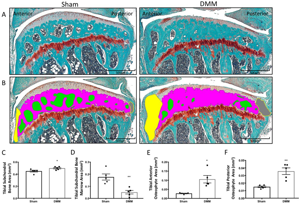
(A) Tibial articular cartilage and subchondral bone stained with Safranin-O/Fast Green. (B) The subchondral bone marrow areas (green), subchondral bone area (magenta), anterior osteophyte area (yellow), and posterior osteophyte area (gray) were traced with computed histomorphometry software. (C–F) Graphed histomorphometric areas between the sham and DMM mice. Compared to the sham mice, DMM mice had an increased tibial subchondral bone area (C) and tibial anterior and posterior osteophyte areas (E–F), as well as decreased tibial subchondral bone marrow area compared to sham mice (D). Images were taken using 4× magnification. *P < 0.05, **P < 0.01 using unpaired t-test with Welch’s correction. Values are expressed as mean ± SEM; n = 5/group.
Figure 3: Histomorphometry of synovium from sham surgery and DMM mice.

(A) Synovium stained with Safranin-O/Fast Green. (B) The synovial thickness was measured by tracing the anterior meniscofemoral synovial membrane across the anterior aspect of the tibiofemoral joint (green). (C) Graphical representation of synovial thickness measurements using computed histomorphometry software. DMM mice had an increased synovial thickness compared to sham mice. Images were taken at 20× magnification. ***P < 0.001 using unpaired t-test with Welch’s correction, values are expressed as mean ± SEM; n = 5/group; S = synovium; F = femur; and M = meniscus.
8. Statistical analysis
Collect the measured parameters and average the results from the three representative sections for each sample. Analyze the data using an unpaired Student’s t-test to compare two groups or one-way ANOVA to compare three or more groups.
-
Display the data as mean ± standard error of mean.
NOTE: Statistical significance was achieved at p ≤ 0.05.
Representative Results
DMM-induced OA results in articular cartilage degeneration and chondrocyte loss
DMM-induced OA resulted in an increased OARSI score compared to sham mice, distinctly characterized by surface erosion and cartilage loss (Figure 1A,D). The histomorphometry protocol detailed here detected several OA-associated changes, including a decrease in total cartilage area and in the uncalcified cartilage area (Figure 1A,B,E,G); reduction in the total chondrocyte number; and, importantly, loss of matrix producing chondrocytes (Figure 1H,I). Changes to the articular surface, indicative of the severity of erosion, were evaluated using the cartilage fibrillation index. Overall, the fibrillation index increased in DMM mice (Figure 1C,K,L). However, it is also important to note that the fibrillation index may decrease in end-stage OA due to complete erosion of the cartilage surface, as discussed in the Protocol. An increase in the fibrillation index signifies degeneration of the articular cartilage surface during OA development and progression. These results highlight the ability of the histomorphometric analysis program to detect and quantify pathological cartilage changes that characterize OA progression.
Assessment of other joint changes in DMM-induced OA
OA affects joint tissues other than the cartilage, and pathological changes in these tissues play a crucial role in disease progression. Here, the described histomorphometric analysis method revealed an increase in the subchondral bone area and a reduction in the area of the bone marrow space in DMM mice (Figure 2A–D), indicating subchondral bone sclerosis29,30. Both anterior and posterior osteophyte areas also increased in DMM mice (Figure 2E,F), suggesting an ongoing subchondral bone remodeling that acts as a compensatory mechanism to handle changes in joint loading at the site of injury29,30.
Histomorphometric analysis of the synovium showed increased synovial thickness in DMM mice (Figure 3A–C), which is a typical outcome of OA-associated synovial inflammation and the diffusion of inflammatory cytokines into the joint space11,12,31,32,33,34.
Analysis of interuser variability between OARSI scoring versus histomorphometry
Figure 4A shows no significant interuser variability of both histomorphometric analysis of the uncalcified cartilage area (Figure 4A) and the OARSI score (Figure 4B). However, the histomorphometric analysis showed an extremely low mean difference in between observers ranging from −0.0001179–0.00120, leading to an almost complete overlap of the results obtained by the three observers, while the mean difference between observers was higher in the OARSI score ranging from −0.3–0.3 with a clear deviation of O1 values from O2 and O3 values.
Figure 4: Interuser variability in OARSI scoring versus histomorphometric analysis.

(A) Uncalcified cartilage area measurements obtained using histomorphometry by three blinded observers (O1, O2, O3). (B) OARSI scores for sham and DMM mice obtained from the three blinded observers. The dotted lines denote the mean value for each group.
Discussion
Recent osteoarthritis research has enhanced our understanding of the crosstalk between the different tissues within the joint and the role each tissue plays in disease initiation or progression8,9,10,35,36. Accordingly, it has become obvious that the assessment of OA should not be limited to analysis of the cartilage but should also include analysis of the subchondral bone and synovium. In spite of that, the articular cartilage has been the primary focus of semiquantitative scoring of OA15,37,38. Although computed histomorphometry has already been applied to various areas of musculoskeletal research39,40,41,42,43,44, there is an unmet gap in describing a protocol to accurately and reproducibly analyze discrete changes to the multitude of tissues within the knee joint compartment during OA. The application of histomorphometric analysis measurements to quantify changes to the cartilage, subchondral bone, and synovium provides a more holistic assessment of the primary and secondary changes in OA joints.
Here, we describe for the first time a detailed protocol that utilizes a computerized and semiautomated histomorphometric analysis software to quantify pathological changes in different joint compartments and evaluate OA development, progression, or regression. Care should be taken during sample preparation, as clear and consistent Safranin-O and Fast Green stains are essential to limit ambiguity when tracing and taking measurements with histomorphometric software. Using fresh staining solutions for each batch of slides is advisable. In addition, slide selection for staining must occur at consistent levels between blocks. The first slide must be taken at a similar level between samples, ideally as soon as the anterior and posterior meniscal horns start separating.
During OA, total cartilage and uncalcified cartilage areas decrease due to cartilage fibrillation and degeneration. In severe OA, complete degeneration of the calcified cartilage may also occur. The protocol highlights the significance of determining the chondrocyte phenotype as an assessment of OA progression for the evaluation of anabolic versus catabolic signaling in cartilage. The total number of chondrocytes and the number of matrix producing chondrocytes (anabolic) are high in normal cartilage and low in OA cartilage, where the majority of existing chondrocytes in OA are matrix nonproducing (catabolic). Importantly, this essential parameter in the field of OA therapeutic discovery is not evaluated by OARSI or Mankin’s scoring systems. Certain interventions that not only preserve the cartilage area and the number of chondrocytes but also promote chondrocyte anabolic phenotype may be more effective therapeutic approaches.
The protocol detailed here also provides a method to quantitatively measure the subtle changes in cartilage surface fibrillations present in mild to moderate OA. A greater number of fibrillations means an increased perimeter measurement due to the presence of indentations in the articular surface. Thus, the tibial articular surface perimeter and fibrillation index are low in normal cartilage, intermediate in mild OA due to some fibrillations, high in moderate OA due to more fibrillations, but again low in severe OA due to complete cartilage degeneration and loss.
Subchondral bone remodeling and sclerosis are characteristic pathological signs of OA, resulting in reduced subchondral marrow space area and increased subchondral bone area8,9,10,29,30. Quantification of changes in the subchondral bone area and subchondral marrow space area described in the protocol demonstrate the importance of understanding multi-tissue changes as a driving component for the complex nature of OA disease development and progression. Measurement of the anterior and posterior osteophyte areas provides important insight into the scale of bone remodeling occurring within the joint. The osteophyte area is extremely small in sham-operated knees and is increased due to osteophyte formation in OA. Measurement of the anterior osteophyte area differed slightly from the measurement of the posterior osteophyte area due to the severe nature of bone remodeling occurring at the medial region of the knee, near the site of DMM injury.
Finally, this protocol outlines a quantifiable assessment of changes in the synovial membrane. Synovial thickness is low in sham joints and increases in OA. Inflammation in OA leads to thickening of the synovial membrane to increase delivery of inflammatory cytokines and other factors to the joint space10,11,12,31,32. Thus, it is essential to evaluate joint inflammation as a modulating factor of OA disease progression.
Use of the histomorphometry software is limited by the availability of the hardware: touchscreen monitors or tablets with a stylus are absolutely necessary given the amount of manual tracing required for taking accurate measurements. Attempting to measure small areas with the histomorphometry software can also be limiting, as the pen size is restricted to one diameter. While this inability to measure small areas may be inconvenient, the joint areas measured are easily defined with the area tool, and the low discrimination of the software makes a negligible difference in the final measurement.
It should also be noted that interuser variability is always an area of concern regarding implementation of a reliable and reproducible quantitative protocol. Establishing an effective, reproducible, and rigorous histomorphometry protocol requires limiting potential compounding variables within the experimental analysis, including reducing interuser variability. However, following a short training session (about 30 min) with the software, lab members were able to generate highly consistent and reproducible measurements, where the distribution of measurements between users reflects more of a direct overlay representing almost no interuser variability. Importantly, this histomorphometry protocol demonstrates an efficient method to quantify even discrete differences between sham samples in a highly reproducible manner.
The OARSI scoring system is a commonly used measure of assessment for cartilage damage in OA patients and experimental murine models15. The scoring system is based on a whole-number scale primarily focused on the extent of clefts/erosion or the articular surface. Although we found no significant interuser variability with the OARSI scores in our experiment, there still was a higher mean difference in between observers, versus almost none in the described histomorphometry protocol. Thus, establishing this reproducible protocol for histomorphometric analysis of defined parameters allows for highly consistent measurements of each sample, even between multiple users, removing some of the subjective nature of sample analysis.
The OARSI standardized scoring system is a benchmark for OA research. However, the limited score-based nature of the system does not allow for quantification of subtle changes occurring within the joint. The expanded joint evaluation described in this manuscript using histomorphometry software provides an enhanced and less subjective characterization of the severity of OA. This protocol is optimized for mice that have undergone a surgical induction of OA. The procedures and techniques can be applied for evaluation of OA within other models and hypotheses, however.
In summary, the protocol detailed here provides a clear guide for a rigorous and reproducible semiautomated quantitative approach to investigate OA pathology or evaluate therapeutic interventions.
Supplementary Material
Supplementary Figure 1: Histological analysis of Safranin-O and Fast Green stained mouse tibiofemoral joint sections. (A) A 4× magnification image of the tibiofemoral joint. Areas of focus are labeled. (B) A 10× magnification image of the tibiofemoral joint ROI. The tibial and femoral surfaces as well as the anterior and posterior meniscal horns are visualized. The menisci are approximately the same size and the imaging ROI is centered on the joint compartment. (C) A 40× magnification image of the proximal tibial surface. The tidemark line is labeled as the line between the uncalcified and calcified cartilage zones. The osteochondral junction is labeled between the end of the calcified cartilage and beginning of the subchondral bone.
Supplementary Figure 2: Histomorphometry system setup and camera white balance calibration. (A) Mouse tibiofemoral joint visualized at 4× magnification in the software window with white balance not set. Note the camera settings tab at the top of the screen and the selection in the dropdown menu to set the white balance. (B) Mouse tibiofemoral joint at 4× magnification with white balance set. Note the change in the coloration and staining of the sample, increasing the user’s ability to distinguish certain areas of the tibiofemoral joint when performing measurements.
Supplementary Figure 3: Setup of histomorphometric software prior to histomorphometric analysis measurements. Representative screenshot of the histomorphometric software window. Note the stained mouse knee section is centered in the measurement region (yellow grid) and the correct magnification scale for the region is selected to match the objective being used on the microscope (circled in red in the top right hand corner of the screen). The list of parameters is displayed in the column to the right of the imaging and measurement area. Selecting a parameter will highlight the parameter, hence Tibial Fibrillation is currently selected to be measured. The Summary Data tab at the bottom of the window is where measurements for each parameter for each sample will be organized and saved to be exported following completion of each parameter measurement for each section.
Acknowledgments
We would like to acknowledge the assistance of the Department of Comparative Medicine staff and the Molecular and Histopathology core at Penn State Milton S. Hershey Medical Center. Funding sources: NIH NIAMS 1RO1AR071968-01A1 (F.K.), ANRF Arthritis Research Grant (F.K.).
Footnotes
Video Link
The video component of this article can be found at https://www.jove.com/video/60991/
Disclosures
None
References
- 1.Ma VY, Chan L, Carruthers KJ Incidence, prevalence, costs, and impact on disability of common conditions requiring rehabilitation in the United States: stroke, spinal cord injury, traumatic brain injury, multiple sclerosis, osteoarthritis, rheumatoid arthritis, limb loss, and back pain. Archives of Physical Medicine and Rehabililation. 95 (5), 986–995 (2014). [DOI] [PMC free article] [PubMed] [Google Scholar]
- 2.Hopman W. et al. Associations between chronic disease, age and physical and mental health status. Journal of Chronic Diseases in Canada. 29 (3), 108–116 (2009). [PubMed] [Google Scholar]
- 3.Lorenz J, Grässel S Experimental osteoarthritis models in mice In Mouse Genetics. Methods in Molecular Biology. ed., Singh S, Coppola V, vol 1194, 401–419, Humana Press; New York, NY: (2004). [DOI] [PubMed] [Google Scholar]
- 4.Sophia Fox AJ, Bedi A, Rodeo SA The basic science of articular cartilage: structure, composition, and function. Journal of Sports Health. 1 (6), 461–468 (2009). [DOI] [PMC free article] [PubMed] [Google Scholar]
- 5.Van der Kraan P, Van den Berg W Chondrocyte hypertrophy and osteoarthritis: role in initiation and progression of cartilage degeneration? Osteoarthritis and Cartilage. 20 (3), 223–232, (2012). [DOI] [PubMed] [Google Scholar]
- 6.Hodsman AB et al. Parathyroid hormone and teriparatide for the treatment of osteoporosis: a review of the evidence and suggested guidelines for its use. Endocrine Reviews. 26 (5), 688–703 (2005). [DOI] [PubMed] [Google Scholar]
- 7.Pitsillides AA, Beier F Cartilage biology in osteoarthritis—lessons from developmental biology. Nature Reviews Rheumatology. 7 (11), 654 (2011). [DOI] [PubMed] [Google Scholar]
- 8.Yuan X. et al. Bone–cartilage interface crosstalk in osteoarthritis: potential pathways and future therapeutic strategies. Osteoarthritis and Cartilage. 22 (8), 1077–1089 (2014). [DOI] [PubMed] [Google Scholar]
- 9.Goldring SR, Goldring MB Changes in the osteochondral unit during osteoarthritis: structure, function and cartilage–bone crosstalk. Nature Reviews Rheumatology. 12 (11), 632 (2016). [DOI] [PubMed] [Google Scholar]
- 10.Martel-Pelletier J. et al. Osteoarthritis. Nature Reviews Disease Primers. 2 (1), 16072 (2016). [DOI] [PubMed] [Google Scholar]
- 11.Goldring MB, Otero M Inflammation in osteoarthritis. Current Opinion in Rheumatology. 23 (5), 471 (2011). [DOI] [PMC free article] [PubMed] [Google Scholar]
- 12.Sellam J, Berenbaum F The role of synovitis in pathophysiology and clinical symptoms of osteoarthritis. Nature Reviews Rheumatology. 6 (11), 625 (2010). [DOI] [PubMed] [Google Scholar]
- 13.Ma H. et al. Osteoarthritis severity is sex dependent in a surgical mouse model. Osteoarthritis and Cartilage. 15 (6), 695–700 (2007). [DOI] [PubMed] [Google Scholar]
- 14.Katon W, Lin EH, Kroenke K The association of depression and anxiety with medical symptom burden in patients with chronic medicalillness. General Hospital Psychiatry. 29 (2), 147–155 (2007). [DOI] [PubMed] [Google Scholar]
- 15.Glasson S, Chambers M, Van Den Berg W, Little C The OARSI histopathology initiative–recommendations for histological assessmentsof osteoarthritis in the mouse. Osteoarthritis and Cartilage. 18, S17–S23 (2010). [DOI] [PubMed] [Google Scholar]
- 16.Pastoureau P, Leduc S, Chomel A, De Ceuninck F Quantitative assessment of articular cartilage and subchondral bone histology in themeniscectomized guinea pig model of osteoarthritis. Osteoarthritis and Cartilage. 11 (6), 412–423 (2003). [DOI] [PubMed] [Google Scholar]
- 17.O’Driscoll SW, Marx RG, Fitzsimmons JS, Beaton DE Method for automated cartilage histomorphometry. Tissue Engineering. 5 (1), 13–23 (1999). [DOI] [PubMed] [Google Scholar]
- 18.Matsui H, Shimizu M, Tsuji H Cartilage and subchondral bone interaction in osteoarthrosis of human knee joint: a histological andhistomorphometric study. Microscopy Research Technique. 37 (4), 333–342 (1997). [DOI] [PubMed] [Google Scholar]
- 19.Hacker SA, Healey RM, Yoshioka M, Coutts RD A methodology for the quantitative assessment of articular cartilagehistomorphometry. Osteoarthritis and Cartilage. 5 (5), 343–355 (1997). [DOI] [PubMed] [Google Scholar]
- 20.Pastoureau P, Chomel A Methods for Cartilage and Subchondral Bone Histomorphometry In Cartilage and Osteoarthritis. Methods in Molecular Medicine. eds., De Ceuninck F, Sabatini M, Pastoureau P, vol. 101, 79–91, Humana Press; New York, NY: (2004). [DOI] [PubMed] [Google Scholar]
- 21.McNulty MA et al. A comprehensive histological assessment of osteoarthritis lesions in mice. Cartilage. 2 (4), 354–363 (2011). [DOI] [PMC free article] [PubMed] [Google Scholar]
- 22.Glasson S, Blanchet T, Morris E The surgical destabilization of the medial meniscus (DMM) model of osteoarthritis in the 129/SvEvmouse. Osteoarthritis and Cartilage. 15 (9), 1061–1069 (2007). [DOI] [PubMed] [Google Scholar]
- 23.Singh SR, Coppola V Mouse Genetics: Methods and Protocols. Humana Press; New York, NY: (2004). [Google Scholar]
- 24.Fang H, Beier F Mouse models of osteoarthritis: modelling risk factors and assessing outcomes. Nature Reviews Rheumatology. 10 (7), 413 (2014). [DOI] [PubMed] [Google Scholar]
- 25.Culley KL et al. Mouse Models of Osteoarthritis: Surgical Model of Posttraumatic Osteoarthritis Induced by Destabilization of the MedialMeniscus In Osteoporosis and Osteoarthritis. Methods in Molecular Biology. eds., Westendorf J, van Wijnen A, vol. 1226, 143–173, Humana Press, New York, NY: (2015). [DOI] [PubMed] [Google Scholar]
- 26.Van der Kraan P Factors that influence outcome in experimental osteoarthritis. Osteoarthritis and Cartilage. 25 (3), 369–375 (2017). [DOI] [PubMed] [Google Scholar]
- 27.Gage GJ, Kipke DR, Shain W Whole animal perfusion fixation for rodents. Journal of Visualized Experiments. (65), e3564 (2012). [DOI] [PMC free article] [PubMed] [Google Scholar]
- 28.Callis G, Sterchi D Decalcification of bone: literature review and practical study of various decalcifying agents. Methods, and their effectson bone histology. Journal of Histotechnology. 21 (1), 49–58 (1998). [Google Scholar]
- 29.Lajeunesse D, Massicotte F, Pelletier JP, Martel-Pelletier J Subchondral bone sclerosis in osteoarthritis: not just an innocent bystander.Modern Rheumatology. 13 (1), 0007–0014 (2003). [DOI] [PubMed] [Google Scholar]
- 30.Li G. et al. Subchondral bone in osteoarthritis: insight into risk factors and microstructural changes. Arthritis Research Therapy. 15 (6), 223 (2013). [DOI] [PMC free article] [PubMed] [Google Scholar]
- 31.Kapoor M, Martel-Pelletier J, Lajeunesse D, Pelletier JP, Fahmi H Role of proinflammatory cytokines in the pathophysiology ofosteoarthritis. Nature Reviews Rheumatology. 7 (1), 33 (2011). [DOI] [PubMed] [Google Scholar]
- 32.Scanzello CR, Goldring SR The role of synovitis in osteoarthritis pathogenesis. Bone. 51 (2), 249–257 (2012). [DOI] [PMC free article] [PubMed] [Google Scholar]
- 33.Benito MJ, Veale DJ, FitzGerald O, van den Berg WB, Bresnihan B Synovial tissue inflammation in early and late osteoarthritis.Annals of the Rheumatic Diseases. 64 (9), 1263–1267 (2005). [DOI] [PMC free article] [PubMed] [Google Scholar]
- 34.De Lange-Brokaar BJ et al. Synovial inflammation, immune cells and their cytokines in osteoarthritis: a review. Osteoarthritis and Cartilage. 20 (12), 1484–1499 (2012). [DOI] [PubMed] [Google Scholar]
- 35.Findlay DM, Kuliwaba JS Bone–cartilage crosstalk: a conversation for understanding osteoarthritis. Bone Research. 4, 16028 (2016). [DOI] [PMC free article] [PubMed] [Google Scholar]
- 36.Lories RJ, Luyten FP The bone–cartilage unit in osteoarthritis. Nature Reviews Rheumatology. 7 (1), 43 (2011). [DOI] [PubMed] [Google Scholar]
- 37.Pritzker KP et al. Osteoarthritis cartilage histopathology: grading and staging. Journal of Osteoarthritis and Cartilage. 14 (1), 13–29 (2006). [DOI] [PubMed] [Google Scholar]
- 38.Hayami T. et al. Characterization of articular cartilage and subchondral bone changes in the rat anterior cruciate ligament transection andmeniscectomized models of osteoarthritis. Bone. 38 (2), 234–243 (2006). [DOI] [PubMed] [Google Scholar]
- 39.Priemel M. et al. Bone mineralization defects and vitamin D deficiency: Histomorphometric analysis of iliac crest bone biopsies andcirculating 25-hydroxyvitamin D in 675 patients. Journal of Bone and Mineral Research. 25 (2), 305–312 (2010). [DOI] [PubMed] [Google Scholar]
- 40.Yukata K. et al. Continuous infusion of PTH 1–34 delayed fracture healing in mice. Scientific Reports. 8 (1), 13175 (2018). [DOI] [PMC free article] [PubMed] [Google Scholar]
- 41.Kawano T. et al. LIM kinase 1 deficient mice have reduced bone mass. Bone. 52 (1), 70–82 (2013). [DOI] [PMC free article] [PubMed] [Google Scholar]
- 42.Zhang L, Chang M, Beck CA, Schwarz EM, Boyce BF Analysis of new bone, cartilage, and fibrosis tissue in healing murineallografts using whole slide imaging and a new automated histomorphometric algorithm. Bone Research. 4, 15037 (2016). [DOI] [PMC free article] [PubMed] [Google Scholar]
- 43.Wu Q. et al. Induction of an osteoarthritis-like phenotype and degradation of phosphorylated Smad3 by Smurf2 in transgenic mice. Arthritis Rheumatism. 58 (10), 3132–3144 (2008). [DOI] [PMC free article] [PubMed] [Google Scholar]
- 44.Hordon L. et al. Trabecular architecture in women and men of similar bone mass with and without vertebral fracture: I. Two-dimensionalhistology. Bone. 27 (2), 271–276 (2000). [DOI] [PubMed] [Google Scholar]
Associated Data
This section collects any data citations, data availability statements, or supplementary materials included in this article.
Supplementary Materials
Supplementary Figure 1: Histological analysis of Safranin-O and Fast Green stained mouse tibiofemoral joint sections. (A) A 4× magnification image of the tibiofemoral joint. Areas of focus are labeled. (B) A 10× magnification image of the tibiofemoral joint ROI. The tibial and femoral surfaces as well as the anterior and posterior meniscal horns are visualized. The menisci are approximately the same size and the imaging ROI is centered on the joint compartment. (C) A 40× magnification image of the proximal tibial surface. The tidemark line is labeled as the line between the uncalcified and calcified cartilage zones. The osteochondral junction is labeled between the end of the calcified cartilage and beginning of the subchondral bone.
Supplementary Figure 2: Histomorphometry system setup and camera white balance calibration. (A) Mouse tibiofemoral joint visualized at 4× magnification in the software window with white balance not set. Note the camera settings tab at the top of the screen and the selection in the dropdown menu to set the white balance. (B) Mouse tibiofemoral joint at 4× magnification with white balance set. Note the change in the coloration and staining of the sample, increasing the user’s ability to distinguish certain areas of the tibiofemoral joint when performing measurements.
Supplementary Figure 3: Setup of histomorphometric software prior to histomorphometric analysis measurements. Representative screenshot of the histomorphometric software window. Note the stained mouse knee section is centered in the measurement region (yellow grid) and the correct magnification scale for the region is selected to match the objective being used on the microscope (circled in red in the top right hand corner of the screen). The list of parameters is displayed in the column to the right of the imaging and measurement area. Selecting a parameter will highlight the parameter, hence Tibial Fibrillation is currently selected to be measured. The Summary Data tab at the bottom of the window is where measurements for each parameter for each sample will be organized and saved to be exported following completion of each parameter measurement for each section.