The impacts of human migration and city lockdowns on specific air pollutants during the COVID-19 outbreak: A spatial perspective

Abstract

The outbreak of COVID-19 continues to bring unprecedented shock to mankind's socioeconomic activities, and to the wider environment. China, as the early epicenter of the pandemic, locked down one-third of its cities in an attempt to prevent the rapid spread of the virus. Human migration patterns have subsequently been radically altered and many regions have seen perceived improvements in air quality during the lockdowns. This study empirically examines the relationship between human migration and air pollution and further evaluates the causal impacts of the lockdowns. A spatial econometric method and a spatial explicit counterfactual framework are employed in this study. The key findings are as follows: i) a considerable amount of variation in AQI, PM₁₀, PM_2.5, and NO₂ concentration can be explained by human migration but we fail to find suggestive evidence in the cases of SO₂ and CO; ii) the implementation of lockdown measures led to a significant reduction in AQI (18.1%), PM_2.5 (22.2%), NO₂ (20.5%), and PM₁₀ (10.7%), but has no meaningful impacts on SO_2, CO and O₃ levels; iii) further analysis indicates that the impacts of lockdown policies varied by control stringency and by regional heterogeneity. Our findings are of great importance for the Chinese government to create a stronger and more coherent framework in its efforts to tackle air pollution.

1. Introduction

While COVID-19 is creating all kinds of chaos for human's socioeconomic activities, for our environment, it is a reprieve (Diffenbaugh et al., 2020). As the early epicenter of the COVID-19 pandemic, China imposed a range of lockdown measures on one-third of its cities in an attempt to reduce the transmission and minimize the impact of the virus (He et al., 2020). In cities under lockdown, inter-jurisdictional borders were closed and populations were confined to their homes, with unnecessary travel within local city areas also banned (Chinazzi et al., 2020; Kraemer et al., 2020; Tian et al., 2020). As could be expected, governmental intervention policies dramatically altered human migration patterns. Human mobility even dropped by 69.85% after the government implemented travel bans (Bao and Zhang, 2020). One side effect of these measures that became apparent was a perceived improvement in air quality (Bao and Zhang, 2020; Cole et al., 2020).

We know that air pollution can lead to pernicious health effects on ((Taghizadeh-Hesary and Taghizadeh-Hesary, 2020, Zeng et al., 2020), including heart attacks, strokes (Shah et al., 2015), diabetes, lung cancer (Guo et al., 2016; Yang et al., 2020), and high blood pressure (Maomao et al., 2018). These have also been identified among the pre-existing medical conditions that raise the chances of death from COVID-19 infection (Coccia, 2020; Cole et al., 2020; Conticini et al., 2020; Ogen, 2020; Petroni et al., 2020; Setti et al., 2020; Travaglio et al., 2020; Wang et al., 2020a,b; Wu et al., 2020; Yao et al., 2020a, b). Humans are suffering from a respiratory virus. Humanity can no longer afford for its air to be polluted. In the context of China, however, 180 of 338 cities at or above prefecture level (APL cities), i.e. 53.4%, failed to meet national air quality standards in 2019.2 The outbreak of COVID-19 brought unprecedented impacts on human activities, and in turn on the environment (Mostafa et al., 2021), which is expected to increase general understanding of current environment conditions and to trigger new strategies for reducing pollution.

In the specific context of the COVID-19 pandemic, both satellite observations and a few quantitative estimates of the changes in air pollution have found supportive evidence that coronavirus-related lockdowns led to a reduction in air pollution(Le Quéré et al., 2020). For example, Finland's Centre for Research on Energy and Clean Air reported that measures to contain the spread of COVID-19 in China produced a 25% drop in CO₂. Europe is now seeing the same drop in air pollution that occurred in China. Scientists from the Royal Netherlands Meteorological Institute (KNMI), using satellites to monitor both weather and pollution over Europe, found that emissions of NO₂ dropped in Paris as well as in Milan and Madrid. There is a growing literature studying and trying to estimate the impact of the pandemic on air pollution. Evidence of reductions in air pollution following the outbreak of the pandemic was found in many regions, such as Egypt (Mostafa et al., 2021), the USA (Liu et al., 2021), the UK (Ropkins and Tate, 2021), and India (Singh et al., 2020; Vadrevu et al., 2020). In the context of China, several recent studies found similar evidence that the variation in air pollution concentration in many regions of China dropped significantly during the pandemic (Bao and Zhang, 2020). A drop in greenhouse gases (GHGs) shows furthermore that the reduction extends beyond traditional air pollutant emissions (Liu et al., 2020).

However, existing studies are insufficient for understanding the overall effects of the coronavirus shutdown. Scientists from around the world are expected to work on more detailed analyses as satellite data or images have many uncertainties (Schwandner et al., 2017). Another reason is that recent emerging studies lose sight on the presence of spillover effects and regional effects in air pollution (Bi and Zeng, 2019; Chen et al., 2016; Du et al., 2020; Feng et al., 2020; Gong and Zhang, 2017; Yue et al., 2019; Zeng et al., 2019, 2021), which may invalidate the results (Kolak and Anselin, 2019). Many questions remain, including: Do spillover effects in air pollution exist in China during the pandemic? And if yes, which model can be considered as the appropriate model for improving the efficiency and accuracy of analysis? Emissions from human-related activities, including road traffic, heating supply etc., have been identified as the dominant sources of air pollution. Another empirical question we specifically aim to address is: Will human migration be a driving factor in variation of air pollution levels during the outbreak? Moreover, lockdown measures taken to mitigate the spread of the virus brought human's production and consumption activity almost to a standstill. Whether there are causal impacts of the lockdowns on air pollution, and if any, what is their extent? Also, which pollutants have seen their levels fall? In addition, what are the likely heterogeneous impacts in cities exhibiting variations across socioeconomic and environmental dimensions? Any answer to these questions must consider the inherently spatially and temporally dynamic, interactive nature of air pollution.

This study thus aims to investigate the impacts of COVID-19 on our atmospheric environment. Specifically, we are to quantify the relationship between the variation in human movements caused by city lockdowns and air pollution concentration during the confinement period by considering the spillover effects on air pollution. In addition, we will investigate the causal impacts of lockdowns on air pollution to increase our understanding of the epidemic's impact on the environment. To achieve these results, two main datasets were used: real-time monitoring human mobility data (intra-/inter-city migrants) extracted from Baidu Maps and sets of air pollution indicators (AQI, SO₂, PM_2.5, PM₁₀, NO₂, CO, and O₃) collected from the China National Environment Monitoring Center . Our data covers 283 Chinese APL cities for the 100 days ranging from 1 January to April 9, 2020. A core challenge for our empirical analysis was that regional diffusion effects may exist in air pollution. We thus used a spatial econometric framework to incorporate these spatiotemporal factors into our model. Another empirical issue in our estimating procedure is that any reduction in air pollution may have been caused by local environment regulations and a reduction in human movements as the result of panic effects or virus effects which went unobserved. To address this endogeneity concern, we develop a difference-in-difference (DID) framework to make a causal inference by means of a natural experiment, which exploits regional and temporal variation in the adoption of lockdown measures.

Our results found, in brief, that: First, a considerable amount of variation in air pollution is explained by population migration. A one-unit (10 million people) increase in inter-city population movements was associated with 305.9%, 69.0%, 250.5%, and 76.8% increases in AQI, PM₁₀, PM_2.5, and NO₂, and a 110.2% decrease in O₃, respectively, but had no meaningful impacts on SO₂ and CO levels. Regression results for intra-city migration offered similar evidence. Second, relative to cities that were not locked down, transmission control measures taken in the cities under lockdown led to a significant reduction in AQI (−18.1%), PM_2.5 (−22.2%), and NO₂ (−20.5%) concentration and a smaller reduction in PM₁₀ (−10.7%), but no significant drop in SO₂ and CO levels. Further analysis revealed that the impacts of the lockdowns varied by control levels and specific pollutants. Complete lockdowns in eleven cities on average reduced AQI, PM_2.5, PM₁₀, and NO₂ by 26.5%, 26.9%, 32.3%, and 68.2%, respectively, relative to the 40 cities that adopted partial lockdown measures. Finally, heterogeneity analysis demonstrated that the effects of lockdown on specific air pollutants varied largely throughout different types of cities with multiple dimensions of attributes.

Our study provides three potential contributions to the literature. The first is its consideration of the inherently spatially and temporally dynamic, interactive nature of air pollution being studied. Many studies have suggested that air pollution has spillover effects and regional impacts. This study investigates the impacts of human migration and lockdown policies on air pollution by incorporating spatial effects into formal causal inference modeling, leading to a deeper understanding of the relationship between coronavirus lockdown and air pollution. The second contribution concerns the identification strategy. An empirical concern is the potential bias and loss of efficiency that can result invalidation when dependence in both space and time are ignored in the causal investigation of the relationship between human mobility and air pollution. A Spatial Autoregressive (SAR) model was used to propel our causal estimation strategy. Turning to a causal exploration that the lockdown had on environmental outcomes is challenging, as well, since the air pollution concentration of a city at any point in time is shaped by various weather conditions and confounding factors like local environmental regulations. We developed a set of SAR-DID models to address this issue. The third is that our findings provide important policy implications for the ongoing discussion of air pollution control in China. Our findings highlight that, to reduce SO₂ and CO concentration, it is important to accelerate the growth of clean energy and continually combat excessive coal consumption in the power and industrial sectors.

This paper is organized as follows. The second section introduces variables and details the empirical strategy. The third section presents our main empirical results. The fourth section presents results on heterogeneous effects with final conclusions and policy implications provided in the fifth section.

2. Materials and methods

2.1. Data and variables

2.1.1. Air pollution

We use air pollution concentration as a measure of air quality. The original dataset was collected from the China National Environment Monitoring Center (http://datacenter.mee.gov.cn/), a real-time monitoring data system operated by the MEE, including the air quality index (AQI) and six other kinds of primary air pollutants. We aggregated the concentrations of daily air pollutants data into weekly values by following (He et al., 2020).

2.1.2. Human migration

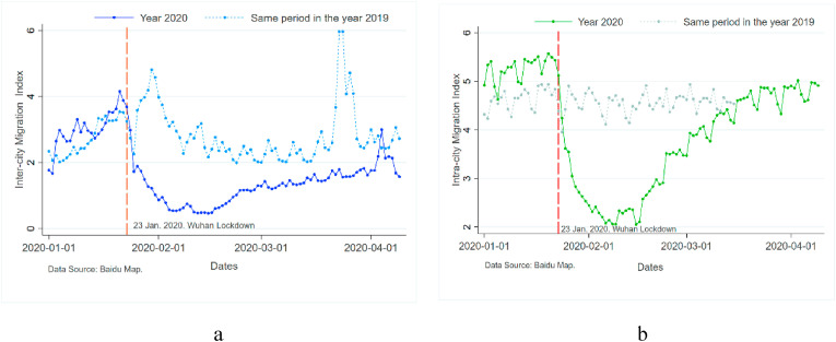
Our data on population migration cover 100 days–1 January to April 9, 2020 – and were obtained from Baidu Maps (https://qianxi.baidu.com/), provided by the dominant Chinese search engine Baidu. This dataset contains two daily migration intensity indices: the inter-city migration intensity index aggregated by the inflow and outflow migration intensity index, and the intra-city migration intensity index. Fig. 1 -a and 1-b plot the overall average variation trend of population migration across 283 Chinese APL cities respectively in 2020 and the same period of 2019, respectively, the latter when adjusted for the lunar calendar. Compared to the same sample period in 2019, the average inter-city and intra-city migration dramatically declined in 2020 after the implementation of the Wuhan lockdown on 23 January.

Fig. 1.

Variation in population migration index in 2020 and 2019. These two figures were plotted with Stata 16.0 software. The intra-city migration data for 2019 is only available through 15 March.

2.1.3. City lockdowns

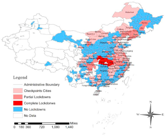
We collected each city's lockdown information from various news media and local government-run websites. To ensure the reliability and validity of the data, we compared our data with the data offered by previous studies for verification purposes (Fang et al., 2020; He et al., 2020). Detailed information of the lockdowns is illustrated in Fig. 2 . Further information about city lockdowns is provided in Table SF-1 (see supplementary files, SF-A) owing to spatial constraints.

Fig. 2.

Cities with different levels of control measures across mainland China. This figure presents the geographic distributions of cities with different levels of lockdown measures. This map was plotted with ArcGIS 10.2 (ESRI) software.

As shown in Fig. 2, by February 12, 2020, 133 of 283 Chinese APL cities (red zones) in 26 provinces had adopted different degrees of lockdown measures. Among them, 11 cities, including Wuhan in Hubei province, announced a total lockdown, which meant that both public and private transportation were suspended, nonessential individual movements in and out of communities were limited, and industrial factories and other public places were closed. 40 cities adopted partial lockdown measures, which meant that most public transportation was suspended, community units in most areas kept only one entrance and exit point open, and each household was allowed limited numbers of entrances and exits. 92 cities set up checkpoints and quarantine zones, which meant that while main line traffic maintained normal operation, people entering and exiting were required to wear masks and receive temperature checks. The rest of the 150 cities (blue zones) were under regular conditions, which meant that local governments in these places did not issue any type of lockdown measures in an official way. This context provides us with a unique opportunity to take advantage of the natural experiments resulting from regional and temporal differences in lockdown policy adoption in various cities to examine the effects of transmission control measures taken in mainland China on air pollution. To test the effects of lockdown measures on air pollution, the dummy variable Treat_lock was coded as 1 when a city had adopted any sort of lockdown policy. Otherwise, it was coded as 0.

2.1.4. Weather conditions

Changes in the concentration levels of pollutants are strongly influenced by multiple meteorological factors. We therefore collected a set of daily weather condition data as our control variables to remove the impact of the local weather conditions on air pollution. Daily history weather data, including maximum and minimum temperatures, maximum wind and gust speeds, and records of rainfall and snow cover, were collected from the website freemeteo.com (https://freemeteo.cn/). This website provides comprehensive weather information for all regions of the world. We collapsed the daily data to weekly city-level datasets according to the same method used to aggregate the air pollution data.

2.1.5. Summary statistics

Table 1 summarizes variables and their definitions, data sources, and summary statistics. Panel A in Table 1 shows descriptive statistics for the seven air pollution indicators selected as our dependent variables and illustrates that there were large variations in air pollution concentrations in different cities. For example, PM_2.5, one of the six major air pollutants, had an average concentration of 46.2 μg/m³, exceeding WHO guidelines and even WHO's least-stringent target (35 μg/m³), with a minimum concentration of 7.369 μg/m³ and a maximum concentration of 238 μg/m³.

Table 1.

Summary statistics.

Variables	Variable definitions	Obs.	Mean	SD	Min	Max
Panel A: Dependent variables
AQI	Air quality index	3962	68.81	35	17.25	262
SO2	SO2 concentrations (μg/m3)	3962	11.48	8	1.745	96
PM2.5	PM2.5 concentrations (μg/m3)	3962	46.2	30	7.369	238
PM10	PM10 concentrations (μg/m3)	3962	68.31	36	13.964	277
NO2	NO2 concentrations (μg/m3)	3962	25.59	13	4.071	84
CO	CO concentrations (mg/m3)	3962	0.85	0	0.205	3
O3	O3 concentrations (μg/m3)	3962	53.45	17	4.649	118
Panel B: Independent variables
Inter-city migrants	The number of Inter-city migrants	3962	153,604	201,914	2195	2,374,810
Intra-city migrants	The number of Intra-city migrants	3962	8,740,000	2,798,460	709,298	16,849,696
Treat_lock	Treat_lock = Event dummy × period dummy. Here event dummy set to 1 if a city adopts lockdown measure during the epidemic, period dummy set to 1 if the time is within the lockdowns.	3962	0.32	0	0	1
Panel C: Control variables
Mintem	Daily maximum temperature (°C)	3962	1.98	9	−24.429	25
Maxtem	Daily minimum temperature (°C)	3962	12.83	9	−14.571	32
Maxwind	Daily maximum steady wind (Km/h)	3962	19.2	5	4.111	44
Maxgust	Daily maximum gust (Km/h)	3962	18.2	14	0	57
Rain	Rainfall(mm)	3962	1.2	2	0	20
Snow	Snow cover(mm)	3962	0.04	0	0	3

Notes: We collected the data presented in Table 1 from official sources from the period of 1 January to 9 April, daily, including: the China National Environment Monitoring Center operated by MEE (http://datacenter.mee.gov.cn/), Baidu Maps (https://qianxi.baidu.com/), local governments-run websites, various media outlets, and Freemeteo (https://freemeteo.cn/). By aggregating and merging these datasets, we obtained a city-week panel of 283 Chinese APL cities, which covers 3962 (283 cities × 14 weeks) observations.

We summarize statistical the results of our independent variables in Panel B, including two population migration indicators and a lockdown dummy variable of our interest. By following Fang et al. (2020), who estimated that one index unit in inter-city and intra-city migration corresponds to 90,848 and 2,182,264 migrants, respectively, we calculated the number of population flow in and out of a city and the number of population travel within a city. We then multiplied these two migration intensity indices by 90,848 and 2,182,264. The average number of intra-city migrants in locked-down cities is significantly lower than that of unlocked-down cities. Additionally, across the 283 cities, 47% of cities implemented lockdown, and travel was restricted for 1249 weeks, accounting for 30% of the sample period.

The bottom of Table 1 shows descriptive statistics for the control variables i.e. weather conditions. The temperature and wind speed values of treated cities is clearly somewhat larger than that of untreated cities.

2.2. Empirical methods

The potential bias and loss of efficiency that can result when spatial effects such as spatial autocorrelation and spatial heterogeneity of air pollution are ignored in the estimation process have been taken into accounts, and all empirical models have been developed within a spatial econometric framework.

2.2.1. Measurements of spatial correlations

The specification of a spatial weighting matrix (represented by W) plays an important role in determining the appropriate form of the spatial model, which summarizes spatial relations among all spatial units. According to Tobler's First Law of Geography (1970), this study calculates an inverse distance weight matrix by using the Euclidean distance from center cell as the measure of the correlation of spatial units. The premise of this weight matrix is that observations further away should have their contributions diminished according to how far away they are. It is calculated as follows:

$$W_{dis}=f\left(\theta ,di{s}_{i,j}\right)$$ (1)

In which $di{s}_{i,j}$ is the distance between spatial unit i and spatial unit i. $\theta$ is the given distance decay parameter.

Earlier research has demonstrated that air pollution has spillover effects and regional impacts among the spatial units (Chen et al., 2016; Zeng et al., 2019). Once released, air pollutants are dispersed by the weather and can travel long distances within and between cities. Emissions from distant and local sources can accumulate into high local concentrations of pollution. To measure such spatial autocorrelation of air pollutants, Global Moran's I Index (GMI) and Local Moran's I Index (LMI), both ranging from −1 (perfect dispersion) to +1 (perfect correlation), are calculated. The formula of GMI is as follows:

$$GMI=\frac{n{\sum }_{i=1}^n{\sum }_{j=1}^n{W}_{dis}(x_i-\bar{x})(x_j-\bar{x})}{({\sum }_{i=1}^n{\sum }_{j=1}^n{W}_{dis}{(x_i-\bar{x})}^2{\sum }_{i=1}^n{(x_i-\bar{x})}^2}\left(i\ne j\right)$$ (2)

where n is the total number of spatial units; x_i and x_j stand for air pollution indicators of i-th and j-th sample cities. ‾x is the sample mean of the variable x, and W_dis is the spatial weight matrix (n × n) of the connection between the i-th and j-th sample cities.

The general form of the LMI can be written as:

$$LM{I}_i=\sum _j{W}_{dis}{Z}_i{Z}_j,(i\ne j)$$ (3)

In which, Z_i and Z_j are the standardized values of air pollution indicators in the i-th and j-th administrative cities, respectively. W_dis have the same meanings as in formula (2).

2.2.2. Human migration and air pollution

It is common practice to consider the SAR specification to account for possible spatial spillover effects in air pollution among different regions. The SAR model assumes the dependent variable is spatially autocorrelated. In our study, we consider air pollutants to be autocorrelated across cities, as explained not only by its associated attributes, but also partially by the traits of the "neighboring" cities. The traits of the "neighbors" are described in terms of contiguity. Compared to traditional spatial econometrics literature, whose literature is interested primarily in the dependence among observations across space, an obvious difference of this study is that we are model both spatial dependence (neighbors, distance, links, etc.) and temporal dependence (time) in the same equation. We assume that air pollution in a certain city is not only explained by its neighbors, but also by its precursors (previous air pollution levels), especially for our city-week data. Thus, considering the spatial effects and time-period specific effects of air pollution, we first employed a dynamic spatial autoregression (SAR) model to investigate the relationship between the population movements and air pollution emissions. Formally, the model is:

$$Ln\left(Ai{r}_{i,t}\right)=\tau \cdot Ln\left(Ai{r}_{i,t-1}\right)+\rho \cdot W\ast Ln\left(Ai{r}_{i,t}\right)+\eta \cdot W\ast Ln\left(Ai{r}_{i,t-1}\right)+\beta \cdot Ln\left(Intercity/Intracit{y}_{i,t}\right)+\lambda \cdot Weathe{r}_{i,t}+cit{y}_i+wee{k}_t+{\epsilon }_{i,t}$$ (4)

We considered three spatial/temporal lag terms to include potential spatial effects of air pollution in Eq. (4). The parameters $\tau$, $\rho$, and $\eta$ are the response parameters of the dependent variable, successively, the dependent variable lagged in time, that is $Ln\left(Ai{r}_{i,t-1}\right)$, which captures the serial dependence between the air pollution of each city over time; the dependent variable lagged in space, that is $W\ast Ln\left(Ai{r}_{i,t}\right)$, which captures the contemporaneous outcomes in neighboring cities; and the dependent variable lagged in both space and time, that is $W\ast Ln\left(Ai{r}_{i,t-1}\right)$, which captures the unobservable spatial and time-period specific effects from neighboring cities. $Ln\left(Intercity/Intracit{y}_{i,t}\right)$ are exogenous explanatory variables of our interest, $Weathe{r}_{i,t}$ is an N × 6 matrix of weather condition variables. $c{\text{ity}}_i$ stands for spatial fixed effects, and $wee{k}_t$ stands for city-by-week fixed effects. ${\epsilon }_{i,t}$ is a disturbance term. This model suggests that the concentration of air pollutants in any given city is a function of the pollution situation both in that city and all the other cities in the system.

2.2.3. Lockdown and air pollution

Even though we have established a link between human movements and air pollution emissions in Eq. (4), it is insufficient for understanding the variation in air pollution during the pandemic. Now we turn to investigate how lockdown affected air quality across China's cities. As the epicenter at the early phase of the pandemic, a range of lockdown measures were imposed on one-third of Chinese cities within days of the Wuhan lockdown. This fact enabled us to identify the causal effects of city lockdown caused by the pandemic and by the air pollution. But a key empirical challenge is the endogeneity of city lockdown originating from various confounding factors that potentially affect the air pollution level. To be specific, the air pollution levels have been declining in most cities over the last several years owing to the government's environmental regulations. As a result, the before-and-after comparison by satellite observation or sensory evidence could simply capture the declining trend in air pollution caused by regulations. Fortunately, our DID strategy helps to address this endogeneity issue because cities without lockdown policies can serve as the counterfactuals, mimicking what would happen in lockdown cities in the absence of its implementation. In our case, some cities were exposed to a lockdown policy (treatment group) and others were not (control group). This background allows us to apply the logic of causal inference and employ a difference-in-difference (DID) method to identify the plausible causal impact of the lockdown policy by comparing how the air pollution concentration in these two groups changed before and after its implementation. Considering the spatial effects inherent in air pollution, we extended the traditional SAR model. Showing how a spatially explicit counterfactual framework can add further insight into the evaluation of treatment effects as shown in Eq. (5).

$$Ln\left(Ai{r}_{i,t}\right)=\rho \cdot TW\ast Ln\left(Ai{r}_{i,t}\right)+\beta \cdot Treat\_loc{k}_{i,t}+\eta \cdot Weathe{r}_{i,t}+cit{y}_i+wee{k}_t+cit{y}_i\ast t+{\epsilon }_{i,t}$$ (5)

In essence, Eq. (5) is a spatial panel model with 283 cross-sectional city observations and 14 time periods, including spatial fixed effects ($cit{y}_i$) and temporal fixed effects ($wee{k}_t$), in which the outcome variable $\text{Ln}\left({\text{Air}}_{i,t}\right)$ is the mean (by week) of the AQI index and the concentration of six air pollutants. The treatment $Treat\_loc{k}_{i,t}$ is the interaction term of the lockdown dummy and the period dummy, which captures the average treatment effect of lockdown measures on air pollution. Other variables and coefficients without specific interpretation are equal to those introduced in function (1). In order to relax common trend assumptions to some extent, we followed the approach of Angrist and Pischke in introducing a city-specific trend as the product of a city dummy with a time trend term t into our model (Angrist and Pischke, 2014).

3. Results and discussion

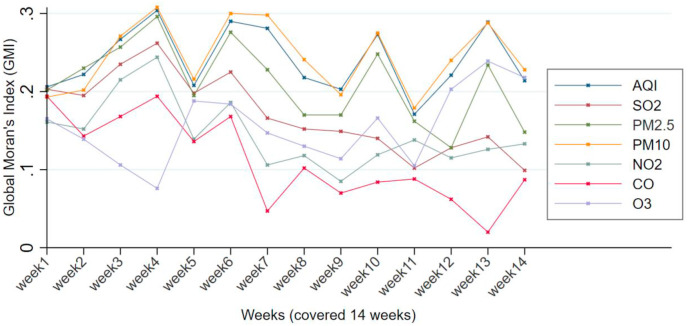
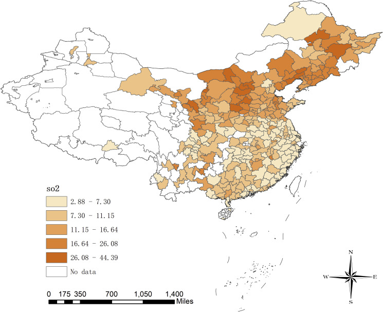
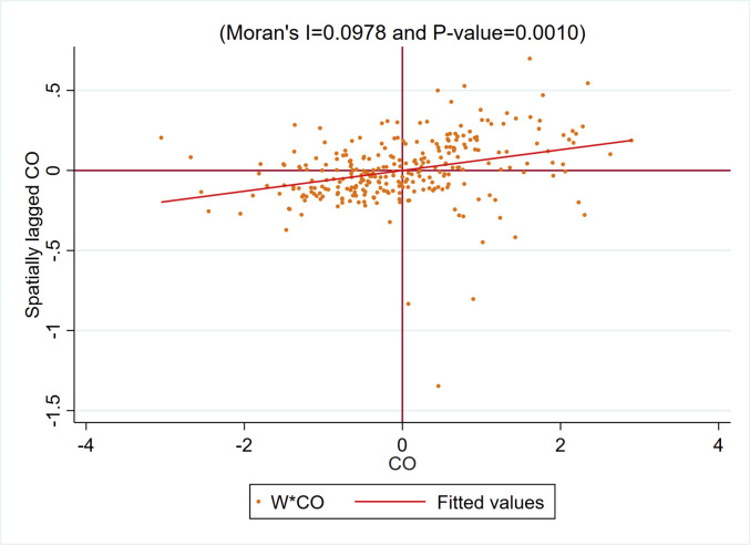
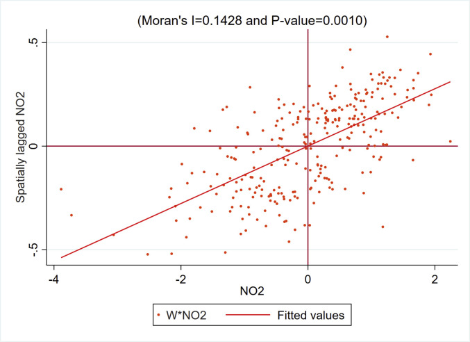
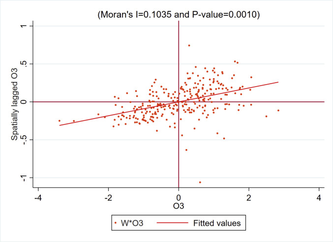
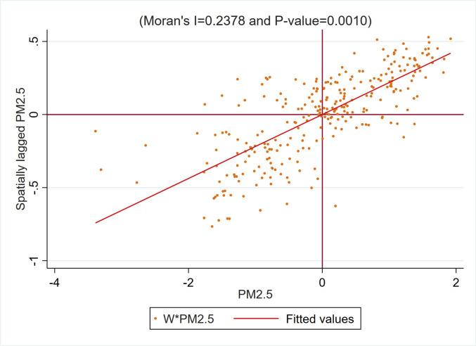
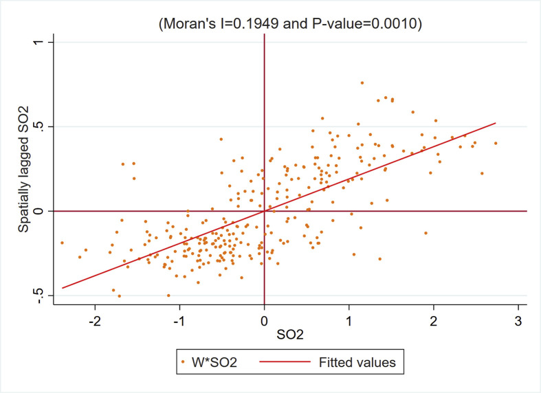
We present our GMI scatter plot for AQI and six air pollutants in Fig. 3 . As illustrated, all GMI of six air pollutants indicators are significantly greater than 0 at the 0.05 confidence level, indicating that air pollution emissions are spatially and positively correlated among the spatial units – the cities with high air pollution emissions (or low air pollution emissions) appear close to each other, or clustered together, in space.

Fig. 3.

GMI scatter plot for AQI and six air pollutants (by week). This figure was plotted with Stata 16.0 software.

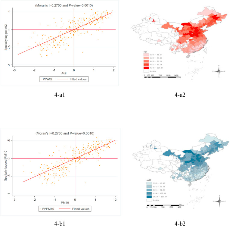
Based on the LMI index, our spatial autocorrelation analysis at the local scale also provides supportive evidence that air pollutants were clustered in space. Fig. 4 presents the Moran scatter plot and geographical distribution of AQI (see Fig. 4-a1 & Fig. 4-a2) and the concentrations of PM₁₀ (see Fig. 4-b1 & Fig. 4-b2). We observed that heavy air pollution was mainly concentrated in northern China. Other pollutants show similar characteristics. To save space, we offer detailed information on the measurements of spatial clustering and heterogeneity of the other five air pollution indicators in supplementary files (SF–B).

Fig. 4.

City-specific Moran scatter plot and geographical distribution for AQI and the concentrations of PM₁₀. These figures were generated with Stata 16.0 software and the map tool in ArcGIS 10.2.

3.1. Correlating human migration and air pollution

3.1.1. Inter-city migration and air pollution

We considered three spatial/temporal lag terms to include potential spatial effects of air pollution and developed a dynamic spatial panel model to capture the effects of population migration on air pollution. For our study, what we require is a model that allows us to estimate which percentage of air pollution changes with human mobility. And a log-linear model, in which the dependent variable is transformed by taking the natural log of it, allows us to interpret these estimated effects in percentage terms. Moreover, the contribution of the spatial model is to breakdown the spatial multiple effects into direct effects, indirect effects and total effects.

We must note that investigating the spatiotemporal patterns and socioeconomic drivers of air pollution by using spatial econometric model is not new. Numerous studies have found evidence for strong spatial overflow effects (indirect effects) and spatial accumulation characteristics in air pollutants among different regions and provided sufficient policy implications such as establishing a regional cooperative governance mechanism. For simplicity, this study thus focuses only on the direct causal relationship between city actions and air pollution which may be more meaningful for local governments when making policies to adapt to the need of their regions. It would, moreover, be overly complicated to report both direct and indirect effects by considering seven proxy indicators of air pollution in the context of spatial econometrics and would reduce the readability of this manuscript.

We report the specific effects incorporating temporal and spatial effects in Table 2 . We begin by interpreting the effects of inter-city migration on air pollution. Both spatial and period fixed effects are included in all models. The estimates show that the coefficients of the lagged dependent variable in time (Ln Air _{i, (t-1)}) and the lagged dependent variable in space (W*ln Air _i, _t) are all positively significant, suggesting that the effects of temporal serial association and the immediate neighbors are to increase air pollution levels, whereas the coefficients of the lagged value in both time and space (W*ln Air _{i, (t-1)}) suggest the opposite. Nevertheless, the presence of the temporal and spatial effects confirms the validity of our selected model. Again, R² and log likelihood of the models suggest that the models fit the data well. As shown at the bottom of Table 2, the dynamic SAR models explain at least 83% of variations in air pollution emissions.

Table 2.

Impact of inter-city migration on air pollution.

Variables	(1) Ln(AQI)	(2) Ln(SO2)	(3) Ln(PM2.5)	(4) Ln(PM10)	(5) Ln(NO2)	(6) Ln(CO)	(7) Ln(O3)
LnAir(t-1)	1.010*** (10.379)	1.003*** (10.567)	1.029*** (10.768)	1.003*** (10.646)	1.037*** (11.572)	1.041*** (9.656)	1.039*** (11.091)
W*lnAirt	0.407*** (13.822)	0.554*** (27.122)	0.378*** (12.564)	0.361*** (11.143)	0.470*** (21.373)	0.470*** (20.836)	0.350*** (17.534)
W*lnAir(t-1)	−0.913*** (−7.314)	−0.773*** (−5.391)	−0.886*** (−7.411)	−0.843*** (−6.272)	−0.774*** (−5.702)	−0.756*** (−5.088)	−0.712*** (−7.560)
Inter-city Migration (directeffects)	3.059** (1.959)	−0.148 (−0.423)	0.690 (0.739)	2.505*** (2.773)	0.768** (2.242)	−0.117 (−0.346)	−1.102*** (−3.426)
Mintem	−0.014*** (−6.486)	−0.026*** (−11.377)	−0.013*** (−5.198)	−0.022*** (−9.20)8	−0.022*** (−11.554)	−0.005*** (−3.482)	−0.007*** (−4.980)
Maxtem	0.012*** (6.729)	0.023*** (12.997)	0.006*** (2.388)	0.021*** (10.494)	0.015*** (9.818)	−0.001*** (−0.953)	0.018*** (13.462)
Maxwind	−0.015*** (−10.735)	−0.010*** (−8.051)	−0.020*** (−12.128)	−0.014*** (−9.290)	−0.014*** (−11.709)	−0.007*** (−7.417)	0.004*** (4.048)
Maxgust	−0.001*** (−2.393)	−0.001*** (−2.412)	−0.001** (−1.994)	−0.002*** (−2.728)	−0.001*** (−2.680)	0.000 (−0.426)	0.000 (0.876)
Rain	−0.010*** (−6.523)	−0.003** (−1.989)	−0.013*** (−6.961)	−0.015*** (−8.162)	−0.003*** (−2.395)	−0.002 (−1.506)	−0.009*** (−7.688)
Snow	0.018* (1.635)	0.011 (1.023)	0.031*** (2.167)	0.023* (1.826)	0.030*** (2.709)	0.016* (1.926)	0.035*** (3.491)
Spatial FE	Yes	Yes	Yes	Yes	Yes	Yes	Yes
Week FE	Yes	Yes	Yes	Yes	Yes	Yes	Yes
Observations	3679	3679	3679	3679	3679	3679	3679
R-squared	0.844	0.904	0.850	0.850	0.901	0.855	0.830
log-likelihood	−109.025	354.602	−702.218	−471.759	649.467	1152.325	1200.267

Notes: t statistics in parentheses, standard errors are clustered at city level (283 clusters) *p < 0.10, indicates significance at 10% levels, **p < 0.05, indicates significance at 5% levels, ***p < 0.01, indicates significance at 1% levels . The matrix W is an inverse distance space weight matrix of dimension 283 × 283 (the same as in the following tables).

Furthermore, we turn our attention toward the coefficients of our explanatory variable and its decomposed marginal effects. The significant and positive coefficients of inter-city migration on AQI, PM_2.5, PM₁₀, and NO₂ imply that human migration among cities may increase the AQI, PM_2.5, PM₁₀, and NO₂ levels, and the corresponding direct effects are 3.059, 0.690, 2.505, and 0.768, implying that a one-unit (10 million people) increase in inter-city population movements is associated with 305.9%, 69.0%, 250.5%, and 76.8% increases in AQI, PM₁₀, PM_2.5, and NO₂, respectively. The lack of significance of the coefficients on SO₂ and CO suggests that inter-city migration has no impact on SO₂ and CO.

The coefficients on O₃ are negative and statistically significant, which seems somewhat counterintuitive. However, this phenomenon is understandable for two reasons. The first relates to O₃'s source and formation. O₃ is not emitted directly into the air, but rather is created by chemical reactions between oxides of nitrogen (NOx) and volatile organic compounds (VOC). O₃ levels occur when precursor emissions (NOx, VOC) react in the presence of sunlight, warm temperatures, and light winds. Unfortunately, we fail to prove whether the precursor emissions affect the O₃ level due to the lack of data for NOx and VOC. The second is that previews studies have found that there is a trade-off between ambient PM_2.5 and O₃ concentrations. For instance, Li et al. (2020) found that O₃ concentrations in the North China Plain are reduced by about 25 ppb(part per billion) relative to PM_2.5-free conditions when PM_2.5 exceeds 80 μg/m³. Another also provides evidence for the negative relations of ambient PM_2.5 and O₃ in cold seasons (December, January and February) in an urban area of East China. These analyses support the inverse relations between O₃ and PM_2.5 in our case(Jia et al., 2017). Nevertheless, we must we must interpret this result with caution because considering chemical reactions will make matters more complicated.

3.1.2. Intra-city migration and air pollution

In Table 3 , we reported the effects of intra-city migration on air pollution. As with the results presented in Table 2, the coefficients of AQI, PM_2.5, PM₁₀, and NO₂ are positive and statistically significant at the 0.01 level, and the predicted direct effects of one-unit change in intra-city migration on these four air pollution indicators are 60.1%, 40.3%, 68.6%, and 33.4%, respectively. The coefficients of O₃ remain negative as before. We again fail to find suggestive evidence for SO₂ and CO.

Table 3.

Impact of intra-city migration on air pollution.

Variables	(1) Ln(AQI)	(2) Ln(SO2)	(3) Ln(PM2.5)	(4) Ln(PM10)	(5) Ln(NO2)	(6) Ln(CO)	(7) Ln(O3)
Intra-city Migration (directeffects)	0.601*** (5.563)	0.027 (0.809)	0.403*** (4.228)	0.686*** (6.340)	0.334*** (10.256)	−0.044 (−1.305)	−0.147*** (−4.598)
Control variables	Yes	Yes	Yes	Yes	Yes	Yes	Yes
Spatial FE	Yes	Yes	Yes	Yes	Yes	Yes	Yes
Week FE	Yes	Yes	Yes	Yes	Yes	Yes	Yes
Observations	3679	3679	3679	3679	3679	3679	3679
R-squared	0.844	0.904	0.850	0.851	0.901	0.854	0.831
log-likelihood	−99.784	355.798	−699.072	−464.089	657.281	1144.931	1208.091

Notes: To save space, the results of the spatial terms and control variables are not reported here, but are available upon request.

The results in Table 2, Table 3 suggest that a considerable amount of the variation in AQI, PM_2.5, PM₁₀, NO₂, and O₃ is partially explained by population migration, while population migration into or within cities does not bear a significant influence on SO₂ and CO emissions. This conclusion is consistent with the fact that PM_2.5, PM₁₀, and NO₂ released from human activity overwhelmingly derive from the raising of dust from road transport and soot from vehicle exhausts, but almost all SO₂ and CO are emitted as a result of the combustion of fossil fuels.

3.2. Quantifying the impact of the lockdown on air pollution

As revealed in the previous section, human movements measured by the human migration intensity index are strongly associated with the concentration of the pollutants PM_2.5, PM₁₀, NO₂, and O₃. However, shedding more light on how human-made activity impacts air pollution is challenging. The exogenous shock in human mobility resulting from lockdown during the COVID-19 outbreak provides a useful research environment for us to examine the potential mechanism between human movements and air pollution emissions. We employ a set of spatial DID estimations to disentangle the lockdown effects on air pollution reductions.

3.2.1. 133 lockdown cities vs. 150 non-lockdown cities

By considering the spatial effects of air pollution, a spatial-autoregression difference-in-difference (SAR-DID) model was considered as a plausible empirical design. For this analysis, we divide our data to create two datasets for two groups over two time periods according to the lockdown information of 283 APL cities. One group (133 cities) is exposed to lockdown policies during one of the time periods (treatment group), while the second group (150 cities) is never exposed to lockdown policies and serves as the control group. Table 4 shows the baseline results for our full sample.

Table 4.

Impact of lockdown on air pollution.

Variables	(1) Ln(AQI)	(2) Ln(SO2)	(3) Ln(PM2.5)	(4) Ln(PM10)	(5) Ln(NO2)	(6) Ln(CO)	(7) Ln(O3)
TW*(LnAiri,t)	0.998*** (1670.617)	0.995*** (850.868)	0.998*** (1670.459)	0.998*** (1670.827)	0.995*** (855.958)	0.997*** (1301.862)	0.997*** (1263.794)
Treat_Lock (direct effects)	−0.181*** (−4.324)	0.017 (0.321)	−0.222*** (−4.380)	−0.107** (−2.175)	−0.205*** (−3.912)	−0.048 (−1.430)	−0.004 (−0.103)
Mintem	−0.022*** (−14.674)	−0.049*** (−24.002)	−0.011*** (−6.100)	−0.038*** (−21.508)	−0.021*** (−10.119)	−0.005*** (−3.673)	−0.018*** (−15.473)
Maxtem	0.018*** (10.487)	0.038*** (16.158)	0.005** (2.152)	0.037*** (18.375)	0.027*** (11.720)	0.002 (1.143)	0.017*** (12.849)
Maxwind	−0.022*** (−18.909)	−0.007*** (−4.583)	−0.030*** (−21.241)	−0.023*** (−17.069)	−0.011*** (−7.163)	−0.008*** (−7.751)	0.006*** (6.528)
Maxgust	0.001 (1.381)	0.001 (1.437)	0.002*** (4.233)	0.000 (−0.338)	−0.002*** (−3.299)	0.000 (−0.584)	0.001*** (3.745)
Rain	−0.024*** (−11.020)	−0.005* (−1.851)	−0.025*** (−9.583)	−0.032*** (−12.425)	−0.011*** (−3.557)	0.002 (1.152)	−0.022*** (−12.717)
Snow	0.006 (0.262)	−0.023 (−0.716)	0.016 (0.553)	−0.001 (−0.034)	0.059* (1.845)	0.036* (1.794)	0.009 (0.507)
Spatial FE	Yes	Yes	Yes	Yes	Yes	Yes	Yes
Week FE	Yes	Yes	Yes	Yes	Yes	Yes	Yes
Constants	0.117*** (2.987)	−0.320*** (−7.170)	0.335*** (7.570)	−0.036 (−0.761)	−0.219*** (−3.537)	0.020 (0.660)	−0.082* (−1.933)
Observations	3962	3962	3962	3962	3962	3962	3962
R-squared	0.527	0.462	0.530	0.493	0.310	0.463	0.556
log-likelihood	−1074.674	−2250.585	−1831.420	−1651.560	−2263.506	−351.280	−88.022

Table 4 reports the baseline SAR-DID regression estimating the extent to which lockdown predicts the variation of air pollution. As demonstrated, the coefficients of Treat_Lock on four of the seven explained variables (i.e. AQI, PM_2.5, PM₁₀, and NO₂) negatively and significantly correlated with lockdown. Average direct effects analysis revealed that −18.1%, −22.2%, −10.7%, and −20.5% of the reduction could be ascribed to the lockdown measures. We fail to find meaningful impacts for SO₂, CO, and O₃. In general, except for O₃, the association between lockdown and air pollution is demonstrated in more than one type of pollutant and is consistent with previous results.

In Table 5 , we test the robustness of the results by applying them to the selection of air pollution indicators. We substituted our explained variable in Table 4 for the 24-h mean value of the six air pollutants and all the estimated results are similar to our earlier benchmark finding based on full samples. Here we failed to re-estimate the AQI due to the lack of 24-h AQI data. Nevertheless, this omission does not affect the conclusion of this paper. AQI, or Air Quality Index, is a system for pollutant concentration measurement. The index formula usually considers up to six main pollutants (PM_2.5, PM₁₀, CO, SO₂, NO₂, and O₃). AQI is thus too general for describing specific effects of air pollution. Additionally, the focus of this paper is the variation of the other six specific air pollutants and we provide a comprehensive analysis for each air pollutant in subsequent sections.

Table 5.

Impact of lockdown on 24-h concentration mean of six air pollutants.

Variables	(2) Ln(SO2_24 h)	(3) Ln(PM2.5_24 h)	(4) Ln(PM10_24 h)	(5) Ln(NO2_24 h)	(6) Ln(CO_24 h)	(7) Ln(O3_24 h)
Treat_Lock (direct effects)	0.014 (0.252)	−0.222*** (−5.025)	−0.118*** (−2.819)	−0.037*** (−3.710)	0.009 (0.498)	0.006 (0.405)
Control variables	Yes	Yes	Yes	Yes	Yes	Yes
Spatial FE	Yes	Yes	Yes	Yes	Yes	Yes
Week FE	Yes	Yes	Yes	Yes	Yes	Yes
Constants	−0.324*** (−7.271)	0.335*** (7.796)	−0.040 (−0.867)	−0.342 (−1.531)	−0.094*** (−2.559)	−0.132*** (−4.716)
Observations	3962	3962	3962	3962	3962	3962
R-squared	0.462	0.528	0.489	0.296	0.585	0.585
log-likelihood	−2249.933	−1817.766	−1629.764	−2291.204	1158.821	1158.821

Notes: To save space, the results of the spatial terms and control variables are not reported here, but are available upon request (the same as in the following tables).

The baseline results demonstrate that, relative to the control group, transmission control measures taken in the cities under lockdown led to a large and significant reduction in AQI, PM_2.5, and NO₂ concentrations and a smaller reduction in PM₁₀, but no significant drop in SO₂, CO, and O₃ levels. These results confirm our earlier findings and are consistent with previous research, as well. In the case of the concentration of SO₂, which did not significantly decline following the lockdown, it likely reflects the fact that China heavily relies on fossil fuels for its energy needs, and the fact that residents burned more coal for heating in the colder period we studied. It is less clear why CO, a pollutant largely emitted from transport, and O₃, a pollutant not directly emitted but rather formed in the air, did not fall following the lockdown.

3.2.2. Stringency of lockdown measures and air pollution

In response to the rapid transmission of COVID-19, different levels of prevention and control measures were imposed on various cities within days of the Wuhan lockdown on 23 January. As the epicenter, eleven cities under the jurisdiction of Hubei province announced complete lockdown, 40 cities adopted partial lockdown measures, and 92 cities set up checkpoints and quarantine zones.

In order to isolate the effects of different degrees of stringency in lockdown measures, we implemented two sets of regression that differ in estimation sample and in the definition of the control group. The estimation sample used in regressions reported in Panel A of Table 6 is taken from the eleven completely locked-down cities (treatment group) and 40 partially locked-down cities (control group). In so doing, we compare the extent of the variation of air pollution in cities under complete lockdown to cities under partial lockdown. As illustrated in Panel A of Table 6, the estimated coefficients on Treat_Lock remain negative for AQI, PM_2.5, PM₁₀, and NO₂, and economically and statistically significant. The estimates suggest that complete lockdown in eleven cities on average reduces AQI, PM_2.5, PM₁₀, and NO₂ by 26.5%, 26.9%, 32.3%, and 68.2%, respectively, relative to the 40 cities that adopted partial lockdown measures. We again fail to find suggestive evidence that lockdown impacts SO₂ concentration. Contrary to our expectation, we find the coefficients for CO and O₃ are positively significant, indicating that the concentrations of CO and O₃ in completely locked-down cities increased by 23.2% and 26.9% when separately compared with partially locked-down cities.

Table 6.

Stringency of lockdown measures and air pollution.

Variables	(1) Ln(AQI)	(2) Ln(SO2)	(3) Ln(PM2.5)	(4) Ln(PM10)	(5) Ln(NO2)	(6) Ln(CO)	(7) Ln(O3)
Panel A: 11 complete lockdown cites vs. 40 partial lockdown cities
Treat_Lock (direct effects)	−0.265*** (−4.471)	−0.077 (1.551)	−0.269*** (−4.001)	−0.323*** (−5.002)	−0.682*** (−10.352)	0.232 *** (6.657)	0.269*** (6.329)
R-squared	0.472	0.598	0.525	0.443	0.437	0.562	0.600
log-likelihood	−150.091	−314.661	−274.650	−243.115	−270.477	74.400	−72.451
Panel B: 11 complete lockdown cites vs. 92 checkpoints cities
Treat_Lock (direct effects)	−0.064 (−1.215)	−0.165*** (−2.897)	−0.019 (−0.317)	−0.101** (−2.012)	−0.421*** (−6.369)	0.171*** (4.283)	0.229*** (6.214)
R-squared	0.502	0.366	0.529	0.453	0.342	0.414	0.570
log-likelihood	−345.021	−739.890	−575.994	−557.696	−769.241	−200.246	−158.799

The estimation sample in Panel B consists of the eleven cities under complete lockdown (treatment group) and 92 cities that set up checkpoints and quarantine zones (control group). As demonstrated in Panel B of Table 6, lockdown measures reduce PM₁₀ and NO₂ by 10.1% and 42.1%, respectively, and the coefficients of Treat_Lock are significant as before. Unexpectedly, we do not observe statistically significant effects for AQI and PM_2.5, suggesting that control measures taken by the eleven completely locked-down cities have no significant impacts on AQI and PM_2.5, with respect to cities that establish checkpoints and insulating areas. We also find that the coefficients of Treat_Lock on CO and O₃ remain positive and statistically significant, which confirm that the concentrations of CO and O₃ increased in completely locked-down cities. The coefficient of SO₂ remains insignificant as before. These results must be interpreted with caution because the sample sizes vary largely in different model settings. Nevertheless, these results highlight that the impacts of the lockdowns varied by control levels and specific pollutants.

4. Heterogeneity analysis

Cities are inherently heterogeneous entities. To gain further insight into the impacts of city lockdown on air pollution better, we turn our focus to understand heterogeneous effects on air pollution from four factors – population distribution, industrial development, winter heating supply, and transportation demand – that are most relevant to this study. We specifically explore heterogeneity between different cities through sub-city typologies based on Eq. (5). In presenting the results, we consider each dimension in turn.

Population density measured by the ratio of total urban population to administrative area is one of the most basic attributes of a city. By comparing the local population density with the national mean value, we divide our estimation sample into two sub-city typologies: 107 cities with high population density and 176 cities with low population density. The results of the statistical analyses are reported in Panels A & B of Table 7 . As revealed, the direct effects of lockdown measures taken in densely populated cities are −7.3%, −10.0%, and −3.8% for AQI, PM_2.5, and PM₁₀, respectively, corresponding to a reduction ratio of −8.7%, −10.7%, and −6.4% in cities with lower population density. These results suggest that lockdown led to a greater improvement in AQI, PM_2.5, and PM₁₀ in populated cities. We curiously observed evidence that lockdown significantly increased SO₂ emission by 6.9% in high-density cities but had no obvious impacts on low-density cities. This finding is consistent with the fact that energy consumption, especially coal consumption for heating and domestic burning, is higher in the cities in which more people are concentrated, combined with the fact that our sample focuses only on the first quarter of 2020, traditionally the coldest season of the year, due to the availability of our data. Results also show that lockdown policies increased NO₂ in both cities with high population density and cities with low population density, and that the variation in densely populated cities is greater than in sparsely populated cities. This disparity was likely to be caused by transportation but weakened the rate of increase in cities with low population density. It is understandable as emissions from anthropogenic activity are relatively stable and more people means more pollution emissions, even if a city is locked down.

Table 7.

Heterogeneity analysis.

Variables	(1) Ln(AQI)	(2) Ln(SO2)	(3) Ln(PM2.5)	(4) Ln(PM10)	(5) Ln(NO2)	(6) Ln(CO)	(7) Ln(O3)
Panel A: 107 cities with high population density (N = 1498)
Treat_Lock (direct effects)	−0.073*** (−4.135)	0.069*** (2.844)	−0.100*** (−4.153)	−0.038 (−1.619)	0.100*** (4.100)	0.005 (0.325)	−0.013 (−0.217)
Panel B: 176 cities with low population density (N = 2464)
Treat_Lock (direct effects)	−0.087*** (−3.242)	−0.007 (−0.009)	−0.107*** (−3.982)	−0.064*** (−2.611)	0.059*** (2.691)	−0.022 (−1.063)	−0.017 (−1.021)
Panel C: 86 cities with more industrial firms (N = 1204)
Treat_Lock (direct effects)	−0.056** (−2.032)	0.024 (0.346)	−0.077*** (−2.585)	−0.025 (−0.321)	0.035 (0.725)	0.021 (0.884)	−0.081*** (−4.082)
Panel D: 197 cities with fewer industrial firms (N = 2758)
Treat_Lock (direct effects)	−0.035** (−2.453)	0.052*** (2.633)	−0.057*** (−2.789)	−0.001 (−0.234)	0.064*** (3.236)	−0.020 (−1.005)	0.020 (1.327)
Panel E: 97 cities with heating supply (N = 1358)
Treat_Lock (direct effects)	−0.096*** (−3.541)	−0.029 (−0.570)	−0.082*** (−2.641)	−0.103*** (−3.341)	0.028 (0.174)	−0.077*** (−3.321)	0.010 (0.613)
Panel F: 186 cities without heating supply (N = 2604)
Treat_Lock (direct effects)	−0.069*** (−2.973)	0.028 (1.043)	−0.092*** (−4.543)	−0.037 (−1.547)	0.106*** (4.368)	−0.023 (−1.443)	−0.041*** (−2.026)
Panel G: 141 cities with a higher transportation demand (N = 1974)
Treat_Lock (direct effects)	−0.092*** (−4.473)	−0.014 (−0.065)	−0.115*** (−4.643)	−0.064** (−2.633)	0.047 (1.445)	−0.045*** (−2.691)	−0.039** (−2.031)
Panel H: 142 cities with a lower transportation demand (N = 1988)
Treat_Lock (direct effects)	−0.028 (−1.203)	0.079*** (3.341)	−0.037 (−1.310)	0.009 (0.774)	0.065*** (2.878)	−0.027 (−1.640)	0.018 (1.548)
Control variables	Yes	Yes	Yes	Yes	Yes	Yes	Yes
Spatial FE	Yes	Yes	Yes	Yes	Yes	Yes	Yes
Week FE	Yes	Yes	Yes	Yes	Yes	Yes	Yes

The most industrialized areas have always been the most polluted. We obtained the numbers of local industrial firms from the China City Statistical Yearbook 2018 to index regional industrial development levels. Specifically, we use the national mean value to divide our estimation sample into high-industrial-intensity cities and low-industrial-intensity cities. The regression results demonstrated that AQI, PM_2.5, and O₃ declined by 5.6%, 7.7%, and 8.1%, respectively, in Panel C, with somewhat smaller decreases (3.5% for AQI, 5.7% for PM_2.5) in Panel D, when these cities adopted lockdown measures. Some of these differences are due to more industrial emissions from power generation, steel, chemicals, and other manufactured products from fossil fuel combustion. Contrary to our expectation, lockdown increased SO₂ and NO₂ concentrations in cities with fewer industrial firms. Cities with more industrial firms recorded a greater reduction in air pollutants, which is likely due to the closure of industrial factories.

In our estimation samples, 97 cities to the north of the Huai River-Qinling Mountains line have received centralized heating supply during cold days each winter, whereas 186 cities to the south have had no access to the heating supply. That China's centralized heating supply heavily relies on coal combustion and inevitably produces serious air pollution is a well-documented fact. Our analysis focuses on these 283 cities and uses the "Huai River-Qinling Mountains" policy to divide our sample into two groups of cities, i.e. those with heating supply and those without heating supply. The regression results are summarized in Panels E & F of Table 7. We find that the effect of lockdown measures varies significantly for specific air pollution indicators across different types of cities. More specifically, the direct effects of lockdown measures taken by colder northern cities are −9.6%, −9.2%, and −10.3% for AQI, PM_2.5, and PM₁₀, respectively, relative to −6.9%, −8.6%, and −3.7% reductions in warmer southern cities. We also found that lockdown reduced CO by 7.7% in heated cities but failed to have an impact on CO level in cities with no heating supply. Additionally, a 10.1% increase in NO₂ and a 4.1% decrease in O₃ was observed in cities with no heating supply. Overall, the observed magnitude of improvement in air quality in colder northern cities is higher than that of warmer southern cities. The difference could be driven by the fact that colder cities consumed more coal for heating, and lockdown reduces such consumption in offices, plants, and schools, which eventually led to a greater improvement in air quality.

Vehicles are one of the major contributors to urban air pollution in China (Fu and Gu, 2017). Based on this fact, this study uses the annual volume of passengers transported by buses and trolley buses data obtained from the City Statistical Yearbook 2018, to measure regional transportation demand. We first calculate the national volume of passengers per city. Then we use the mean value to separate our sample into two groups of 141 cities with a higher transportation demand and 142 cities with a lower transportation demand. Panels G & H of Table 7 illustrate the changes in seven air pollutant indicators for each group. In Panel G, the direct effects of the adoption of quarantine measures are −9.2%, −11.5%, −6.4%, −4.5%, and −3.9% for AQI, PM_2.5, PM10, CO, and O₃, respectively, in cities with a greater traffic demand, but we fail to find meaningful impacts on corresponding indicators in cities with a lower transportation demand in Panel G. The difference possibly owes to the fact that transportation demand is concentrated in heavily polluted areas like the 44 cities located in the Beijing-Tianjin-Hebei metropolitan circle and its surroundings, where the number of buses/trolley buses and taxis under operation are 1,233,289 and 232,742, respectively, making up 21.91% and 25.76% of the total. On the contrary, a 7.9% increase in SO₂ and a 6.5% increase in NO₂ occurred in cities with a relatively lower transportation demand. Cities with a higher transportation demand witnessed a greater reduction in air pollutants, which is likely due to the suspension of private or public transportation.

5. Conclusion and policy recommendations

In this paper we examine the causal relationship between human migration and air pollution, and in turn the casual impacts of lockdown policies on air quality improvement. Considering the regional diffusion effects of air pollution and potential endogeneity concern of city lockdowns, a dynamic SAR model and spatial counterfactual SAR-DID model were employed. We provide novel causal evidence that human migration affects air pollution concentration. Larger population migration, conducive to more intra-/inter-city migrants, is associated with a larger AQI index and higher PM_2.5, PM₁₀, and NO₂ pollution concentration, but has no meaningful impacts on SO₂ and CO levels. A further causal inference provides similar supportive evidence that the adoption of lockdown policies led to a large and significant reduction in AQI (18.1%), PM_2.5 (22.2%), and NO₂ (20.5%) concentrations, and a smaller reduction in PM₁₀ (10.7%), but had no discernible impact on the concentrations of SO₂, CO and O₃. Results also highlight that the impact of the lockdown varied by control stringency and specific pollutants. Sets of heterogeneity analyses by sample indicate that the impact of city lockdown on air quality is more considerable in cities with a low population density, more industrial firms, higher transportation demand, and a heating-supply system. Our findings are particularly important for China as the country strives to improve air quality and accelerate key measures for the development of a more ecological civilization.

This study provides a few policy implications for the practice of air pollution control. Taken together, the results of the study indicate that the emissions of PM₁₀, PM_2.5, and NO₂ are strongly associated with human migration. Further analysis provides similar supportive evidence that the implementation of lockdown measures that have changed human migration patterns also led to a significant reduction in PM_2.5, NO₂, and PM₁₀. There is no denying that air pollutants are released into the atmosphere mainly from road transportation, business activities, and public buildings. An obvious and feasible option for policymakers in cities with higher PM_2.5, NO₂, and PM₁₀ emissions is the adoption of measures like travel restrictions to reduce emissions. Similar measures were already adopted during the Beijing Olympics (2008) and APEC conference (2014), which proved the effectiveness of such restrictive measures. Curiously, we fail to find suggestive evidence in the cases of SO₂ and CO, both of which are mainly emitted by fossil energy combustion. An important policy implication to be learned from these results is that in cities with higher SO₂ and CO emissions, addressing excessive fossil-fuel energy consumption in the power and industry sectors is essential. Finally, heterogeneity analysis confirms that densely-populated, industrial-intensive, and heating-supply cities, and those cities with a high traffic burdens, are important sources of air pollution and highlight the necessity of controlling emissions from these sources when lockdown measures are lifted.

Credit author statement

Jingjing Zeng, Conceptualization, Methodology, Formal analysis, Investigation, Writing – review & editing, Supervision, Project administration, Funding acquisition support. Rui Bao, Data curation, Formal analysis, Investigation, Writing – original draft, Resources, Visualization.

Declaration of competing interest

The authors declare that they have no known competing financial interests or personal relationships that could have appeared to influence the work reported in this paper.

Appendix A. Supplementary data

The following is the Supplementary data to this article:

The supplementary files is available on the website: list of the cities adopted different stringency of lockdown measures (SF-A), details of spatial autocorrelation analysis at local scale (SF–B).

Fig. S1.

Fig. S2.

Fig. S3.

Fig. S4.

Fig. S5.

Fig. S6.

Fig. S7.

Fig. S8.

Fig. S9.

Fig. S10.

References

- Angrist J., Pischke J.S. Mastering 'metrics: the path from cause to effect. Eur. Rev. Agric. Econ. 2014;42:703–705. [Google Scholar]
- Bao R., Zhang A. Does lockdown reduce air pollution? Evidence from 44 cities in northern China. Sci. Total Environ. 2020;731:139052. doi: 10.1016/j.scitotenv.2020.139052. [DOI] [PMC free article] [PubMed] [Google Scholar]
- Bi C., Zeng J. Nonlinear and spatial effects of tourism on carbon emissions in China: a spatial econometric approach. Int. J. Environ. Res. Publ. Health. 2019;16:3353. doi: 10.3390/ijerph16183353. [DOI] [PMC free article] [PubMed] [Google Scholar]
- Chen X., Shuai S., Tian Z., Zhen X., Peng Y. Impacts of air pollution and its spatial spillover effect on public health based on China's big data sample. J. Clean. Prod. 2016;142:915–925. [Google Scholar]
- Chinazzi M., Davis J.T., Ajelli M., Gioannini C., Litvinova M., Merler S., Pastore Y Piontti A., Mu K., Rossi L., Sun K., Viboud C., Xiong X., Yu H., Halloran M.E., Longini I.M., Vespignani A. The effect of travel restrictions on the spread of the 2019 novel coronavirus (COVID-19) outbreak. Science. 2020:a9757. doi: 10.1126/science.aba9757. [DOI] [PMC free article] [PubMed] [Google Scholar]
- Coccia M. medRxiv; 2020. Two Mechanisms for Accelerated Diffusion of COVID-19 Outbreaks in Regions with High Intensity of Population and Polluting Industrialization: the Air Pollution-To-Human and Human-To-Human Transmission Dynamics; pp. 2020–2024. [Google Scholar]
- Cole M.A., Ozgen C., Strobl E. Air pollution exposure and Covid-19 in Dutch municipalities. Environ. Resour. Econ. 2020;76:581–610. doi: 10.1007/s10640-020-00491-4. [DOI] [PMC free article] [PubMed] [Google Scholar]
- Conticini E., Frediani B., Caro D. Can atmospheric pollution be considered a co-factor in extremely high level of SARS-CoV-2 lethality in Northern Italy? Environ. Pollut. 2020;261:114465. doi: 10.1016/j.envpol.2020.114465. [DOI] [PMC free article] [PubMed] [Google Scholar]
- Diffenbaugh N.S., Field C.B., Appel E.A., Azevedo I.L., Baldocchi D.D., Burke M., Burney J.A., Ciais P., Davis S.J., Fiore A.M., Fletcher S.M., Hertel T.W., Horton D.E., Hsiang S.M., Jackson R.B., Jin X., Levi M., Lobell D.B., McKinley G.A., Moore F.C., Montgomery A., Nadeau K.C., Pataki D.E., Randerson J.T., Reichstein M., Schnell J.L., Seneviratne S.I., Singh D., Steiner A.L., Wong-Parodi G. The COVID-19 lockdowns: a window into the Earth System. Nature Rev. Earth Environ. 2020;1:470–481. [Google Scholar]
- Du X., Jin X., Zucker N., Kennedy R., Urpelainen J. Transboundary air pollution from coal-fired power generation. J. Environ. Manag. 2020;270:110862. doi: 10.1016/j.jenvman.2020.110862. [DOI] [PubMed] [Google Scholar]
- Fang H., Wang L., Yang Y. Human mobility restrictions and the spread of the Novel Coronavirus (2019-nCoV) in China. J Public Econ. 2020;191:104272. doi: 10.1016/j.jpubeco.2020.104272. [DOI] [PMC free article] [PubMed] [Google Scholar]
- Feng T., Du H., Lin Z., Zuo J. Spatial spillover effects of environmental regulations on air pollution: evidence from urban agglomerations in China. J. Environ. Manag. 2020;272:110998. doi: 10.1016/j.jenvman.2020.110998. [DOI] [PubMed] [Google Scholar]
- Fu S., Gu Y. Highway toll and air pollution: evidence from Chinese cities. Journal of Environ. Resour. Econ. 2017;83:32–49. [Google Scholar]
- Gong Z., Zhang X. Assessment of urban air pollution and spatial spillover effects in China: cases of 113 key environmental protection cities. J. Resour. Ecol. 2017;8:584–594. [Google Scholar]
- Guo Y., Zeng H., Zheng R., Li S., Barnett A.G., Zhang S., Zou X., Huxley R., Chen W., Williams G. The association between lung cancer incidence and ambient air pollution in China: a spatiotemporal analysis. Environ. Resour. 2016;144:60–65. doi: 10.1016/j.envres.2015.11.004. [DOI] [PubMed] [Google Scholar]
- He G., Pan Y., Tanaka T. The short-term impacts of COVID-19 lockdown on urban air pollution in China. Nat. Sustain. 2020;3:1005–1011. [Google Scholar]
- Jia M., Zhao T., Cheng X., Gong S., Zhang X., Tang L., Liu D., Wu X., Wang L., Chen Y. Inverse relations of PM2.5 and O3 in air compound pollution between cold and hot seasons over an urban area of East China. Atmosphere-Basel. 2017;8:59. [Google Scholar]
- Kolak M., Anselin L. A spatial perspective on the econometrics of program evaluation. Int. Regional. Sci. Rev. 2019;43:1286157918. [Google Scholar]
- Kraemer M.U.G., Yang C., Gutierrez B., Wu C., Klein B., Pigott D.M., du Plessis L., Faria N.R., Li R., Hanage W.P., Brownstein J.S., Layan M., Vespignani A., Tian H., Dye C., Pybus O.G., Scarpino S.V. The effect of human mobility and control measures on the COVID-19 epidemic in China. Science. 2020:b4218. doi: 10.1126/science.abb4218. [DOI] [PMC free article] [PubMed] [Google Scholar]
- Le Quéré C., Jackson R.B., Jones M.W., Smith A.J.P., Abernethy S., Andrew R.M., De-Gol A.J., Willis D.R., Shan Y., Canadell J.G., Friedlingstein P., Creutzig F., Peters G.P. Temporary reduction in daily global CO2 emissions during the COVID-19 forced confinement. Nat. Clim. Change. 2020:647–653. [Google Scholar]
- Liu Q., Harris J.T., Chiu L.S., Sun D., Houser P.R., Yu M., Duffy D.Q., Little M.M., Yang C. Spatiotemporal impacts of COVID-19 on air pollution in California. USA. Sci. Total Environ. 2021;750:141592. doi: 10.1016/j.scitotenv.2020.141592. [DOI] [PMC free article] [PubMed] [Google Scholar]
- Liu Z., Ciais P., Deng Z., Lei R., Davis S.J., Feng S., Zheng B., Cui D., Dou X., Zhu B., Guo R., Ke P., Sun T., Lu C., He P., Wang Y., Yue X., Wang Y., Lei Y., Zhou H., Cai Z., Wu Y., Guo R., Han T., Xue J., Boucher O., Boucher E., Chevallier F., Tanaka K., Wei Y., Zhong H., Kang C., Zhang N., Chen B., Xi F., Liu M., Bréon F., Lu Y., Zhang Q., Guan D., Gong P., Kammen D.M., He K., Schellnhuber H.J. Near-real-time monitoring of global CO2 emissions reveals the effects of the COVID-19 pandemic. Nat. Commun. 2020;11:5172. doi: 10.1038/s41467-020-18922-7. [DOI] [PMC free article] [PubMed] [Google Scholar]
- Maomao Cao, Wanqing Chen. Epidemiology of lung cancer in China. Thorac. Cancer. 2018;6:209–215. doi: 10.1111/1759-7714.12169. [DOI] [PMC free article] [PubMed] [Google Scholar]
- Mostafa M.K., Gamal G., Wafiq A. The impact of COVID 19 on air pollution levels and other environmental indicators - a case study of Egypt. J. Environ. Manag. 2021;277:111496. doi: 10.1016/j.jenvman.2020.111496. [DOI] [PMC free article] [PubMed] [Google Scholar]
- Ogen Y. Assessing nitrogen dioxide (NO2) levels as a contributing factor to coronavirus (COVID-19) fatality. Sci. Total Environ. 2020;726:138605. doi: 10.1016/j.scitotenv.2020.138605. [DOI] [PMC free article] [PubMed] [Google Scholar]
- Petroni M., Hill D., Younes L., Barkman L., Howard S., Howell I.B., Mirowsky J., Collins M.B. Hazardous air pollutant exposure as a contributing factor to COVID-19 mortality in the United States. Environ. Res. Lett. 2020;15:940a–949a. [Google Scholar]
- Ropkins K., Tate J.E. Early observations on the impact of the COVID-19 lockdown on air quality trends across the UK. Sci. Total Environ. 2021;754:142374. doi: 10.1016/j.scitotenv.2020.142374. [DOI] [PMC free article] [PubMed] [Google Scholar]
- Schwandner F.M., Gunson M.R., Miller C.E., Carn S.A., Eldering A., Krings T., Verhulst K.R., Schimel D.S., Nguyen H.M., Crisp D. Spaceborne detection of localized carbon dioxide sources. Science. 2017;358:192. doi: 10.1126/science.aam5782. [DOI] [PubMed] [Google Scholar]
- Setti L., Passarini F., De Gennaro G., Baribieri P., Perrone M.G., Borelli M., Palmisani J., Di Gilio A., Torboli V., Pallavicini A., Ruscio M., Piscitelli P., Miani A. medRxiv; 2020. SARS-Cov-2 RNA Found on Particulate Matter of Bergamo in Northern Italy: First Preliminary Evidence; pp. 2020–2024. [DOI] [PMC free article] [PubMed] [Google Scholar]
- Shah A.S.V., Lee K.K., McAllister D.A., Hunter A., Nair H., Whiteley W., Langrish J.P., Newby D.E., Mills N.L. Short term exposure to air pollution and stroke: systematic review and meta-analysis. BMJ. 2015;350:h1295. doi: 10.1136/bmj.h1295. [DOI] [PMC free article] [PubMed] [Google Scholar]
- Singh V., Singh S., Biswal A., Kesarkar A., Mor S., Khaiwal R. Diurnal and temporal changes in air pollution during COVID-19 strict lockdown over different regions of India. Environ. Pollut. 2020;266:115368. doi: 10.1016/j.envpol.2020.115368. [DOI] [PMC free article] [PubMed] [Google Scholar]
- Taghizadeh-Hesary F., Taghizadeh-Hesary F. The impacts of air pollution on health and economy in Southeast Asia. Energies. 2020;13:1812. [Google Scholar]
- Tian H., Liu Y., Li Y., Wu C., Chen B., Kraemer M.U.G., Li B., Cai J., Xu B., Yang Q.B., Yang P., Cui Y., Song Y., Zheng P., Wang Q., Bjornstad O.N., Yang R., Grenfell B.T., Pybus O.G., Dye C. An investigation of transmission control measures during the first 50 days of the COVID-19 epidemic in China. Science. 2020:b6105. doi: 10.1126/science.abb6105. [DOI] [PMC free article] [PubMed] [Google Scholar]
- Travaglio M., Yu Y., Popovic R., Selley L., Leal N.S., Martins L.M. medRxiv; 2020. Links between Air Pollution and COVID-19 in England; pp. 2020–2024. [DOI] [PMC free article] [PubMed] [Google Scholar]
- Vadrevu K.P., Eaturu A., Biswas S., Lasko K., Sahu S., Garg J.K., Justice C. Spatial and temporal variations of air pollution over 41 cities of India during the COVID-19 lockdown period. Science Rep-UK. 2020;10:16574. doi: 10.1038/s41598-020-72271-5. [DOI] [PMC free article] [PubMed] [Google Scholar]
- Wang B., Liu J., Fu S., Xu X., Li L., Ma Y., Zhou J., Yao J., Liu X., Zhang X., He X., Yan J., Shi Y., Ren X., Niu J., Luo B., Zhang K. medRxiv; 2020. An Effect Assessment of Airborne Particulate Matter Pollution on COVID-19: A Multi-City Study in China; pp. 2020–2024. [Google Scholar]
- Wang P., Chen K., Zhu S., Wang P., Zhang H. Severe air pollution events not avoided by reduced anthropogenic activities during COVID-19 outbreak. Resour. Conserv. Recycl. 2020;158:104814. doi: 10.1016/j.resconrec.2020.104814. [DOI] [PMC free article] [PubMed] [Google Scholar]
- Wu X., Nethery R., Benjamin M., Braun D., Dominici F. medRxiv; 2020. Exposure to Air Pollution and COVID-19 Mortality in the United States: A Nationwide Cross-Sectional Study; pp. 2020–2024. [Google Scholar]
- Yang R., He M., Wang D., Ye R., Li L., Deng R., Shah M., Yeung S.J. Association of cancer screening and residing in a coal-polluted East Asian region with overall survival of lung cancer patients: a retrospective cohort study. Science Rep-UK. 2020;10:17432. doi: 10.1038/s41598-020-74082-0. [DOI] [PMC free article] [PubMed] [Google Scholar]
- Yao Y., Pan J., Liu Z., Meng X., Wang W., Kan H., Wang W. medRxiv; 2020. Ambient Nitrogen Dioxide Pollution and Spread Ability of COVID-19 in Chinese Cities; pp. 2020–2023. [Google Scholar]
- Yue W., Jingyou W., Mei Z., Lei S. Spatial correlation analysis of energy consumption and air pollution in Beijing-Tianjin-hebei region. Energy Procedia. 2019;158:4280–4285. [Google Scholar]
- Zeng J., Liu T., Feiock R., Li F. The impacts of China's provincial energy policies on major air pollutants: a spatial econometric analysis. Energy Pol. 2019;132:392–403. [Google Scholar]
- Zeng J., Jiang M., Yuan M. Environmental risk perception, risk culture, and pro-environmental behavior. Int. J. Environ. Res. Publ. Health. 2020;17:1750. doi: 10.3390/ijerph17051750. [DOI] [PMC free article] [PubMed] [Google Scholar]
- Zeng J., Wen Y., Bi C., Feiock R. Effect of tourism development on urban air pollution in China: the moderating role of tourism infrastructure. J. Clean. Prod. 2021;280:124397. [Google Scholar]
Associated Data
This section collects any data citations, data availability statements, or supplementary materials included in this article.