3D Cine Phase-Contrast MRI at 3T in Intracranial Aneurysms Compared with Patient-Specific Computational Fluid Dynamics

P van Ooij; JJ Schneiders; HA Marquering; CB Majoie; E van Bavel; AJ Nederveen

doi:10.3174/ajnr.A3484

. 2013 Sep;34(9):1785–1791. doi: 10.3174/ajnr.A3484

3D Cine Phase-Contrast MRI at 3T in Intracranial Aneurysms Compared with Patient-Specific Computational Fluid Dynamics

P van Ooij ^a,^b,^✉, JJ Schneiders ^a, HA Marquering ^a,^b, CB Majoie ^a, E van Bavel ^a, AJ Nederveen ^a

PMCID: PMC7965648 PMID: 23598829

Abstract

BACKGROUND AND PURPOSE:

CFD has been proved valuable for simulating blood flow in intracranial aneurysms, which may add to better rupture risk assessment. However, CFD has drawbacks such as the sensitivity to assumptions needed for the model, which may hinder its clinical implementation. 3D PC-MR imaging is a technique that enables measurements of blood flow. The purpose of this study was to compare flow patterns on the basis of 3D PC-MR imaging with CFD estimates.

MATERIALS AND METHODS:

3D PC-MR imaging was performed in 8 intracranial aneurysms. Two sets of patient-specific inflow boundaries for CFD were obtained from a separate 2D PC-MR imaging sequence (2D CFD) and from the 3D PC-MR imaging (3D CFD) data. 3D PC-MR imaging and CFD were compared by calculation of the differences between velocity vector magnitudes and angles. Differences in flow patterns expressed as the presence and strengths of vortices were determined by calculation of singular flow energy.

RESULTS:

In systole, flow features such as vortex patterns were similar. In diastole, 3D PC-MR imaging measurements appeared inconsistent due to low velocity-to-noise ratios. The relative difference in velocity magnitude was 67.6 ± 51.4% and 27.1 ± 24.9% in systole and 33.7 ± 21.5% and 17.7 ± 10.2% in diastole for 2D CFD and 3D CFD, respectively. For singular energy, this was reduced to 15.5 ± 13.9% at systole and 19.4 ± 17.6% at diastole (2D CFD).

CONCLUSIONS:

In systole, good agreement between 3D PC-MR imaging and CFD on flow-pattern visualization and singular-energy calculation was found. In diastole, flow patterns of 3D PC-MR imaging differed from those obtained from CFD due to low velocity-to-noise ratios.

Despite a decrease in fatalities of subarachnoid hemorrhage caused by intracranial aneurysm rupture in recent years,¹ this devastating event is lethal in one-third² to 50%³ of patients. Treatment of incidentally found unruptured aneurysms consists of endovascular coiling or surgical clipping, with procedure-related morbidity and mortality rates slightly in favor of the former.⁴ Because the risk of treatment potentially outweighs the risk of rupture,⁵ treatment decisions should be based on as much available information on the individual aneurysm as possible. It is widely believed that intra-aneurysmal hemodynamics contributes substantially to rupture risk assessment and treatment-planning assistance.^6–9 Many studies showed promising results when conducting assessment of risk factors such as intra-aneurysmal flow patterns and wall shear stress by using patient-specific CFD.^10–12 A drawback of performing CFD is the difficulty in converting large amounts of patient-specific data into workable models.⁹ Without patient-specific data for inflow and outflow boundary conditions, assumptions have to be made regarding heart rate and blood flow, the shape of the inlet-velocity profile, and flow-division ratios in the outflow branches.¹⁴ Further drawbacks are the need for large computational power and extensive calculation time. Despite these drawbacks, CFD has recently been used to associate intra-aneurysmal hemodynamics with rupture.¹⁵

The enormous advancements in MR imaging technology in the past decade now allow direct measurement of intra-aneurysmal flow by using 3D PC-MR imaging.¹⁹ Moreover, the technique was validated against CFD in a real-size phantom.¹⁶ However, clinical application of 3D PC-MR imaging in intracranial aneurysms is complicated by the requirements for high-resolution, high SNR, and patient-tolerable scanning times. In this study, a 3D PC-MR imaging sequence with a scanning duration of approximately 10 minutes, therefore clinically feasible, was applied to 8 intracranial aneurysms. The results were compared with patient-specific CFD simulations in which spatial and temporal boundary conditions obtained from a separate 2D PC-MR imaging and from the 3D PC-MR imaging acquisition were applied. Comparison was performed on a voxel-by-voxel basis by calculating the mean and SD of the paired differences of velocity magnitude and singular energy. The purpose of this study was to assess whether the results of 3D PC-MR imaging and patient-specific CFD are comparable and whether 3D PC-MR imaging can measure important quantitative and qualitative features of intra-aneurysmal flow.

Materials and Methods

Population

The patients were included in a larger study on intra-aneurysmal hemodynamics. Inclusion criteria for that study were a minimal aneurysm size of approximately 3 mm, adult age (18–75 years), and a requirement that patients be enrolled in a diagnostic aneurysm work-up with at least 3D rotational angiography. The patients met a Glasgow Outcome Scale score of ≥4.¹⁷ Patients were excluded if they had contraindications for either 3D-RA or MR imaging. Further inclusion requirement for this study was a successful 3D PC-MR imaging measurement in an unruptured intracranial aneurysm. The local ethics committee approved the study protocol, and written informed consent was obtained from all participating patients. The age of the patients ranged between 44 and 65 years with a mean of 51 ± 7.7 years. Five patients were female; 3 patients were male. The dimensions of the aneurysms were determined on the 3D-RA data by using 3D Slicer (www.slicer.org) and are listed in On-line Table 1.

MR Imaging

The protocol consisted of 3 MR imaging sequences that were conducted on a 3T scanner (Intera; Philips Healthcare, Best, the Netherlands) by using an 8-channel head coil.

First, a high-resolution time-of-flight sequence was performed with a scan resolution of 0.39 × 0.6 × 1 mm, interpolated to 0.39 × 0.39 × 0.5 mm. Imaging parameters were the following: TE/TR/flip angle, 4.2/21.4 ms/20°; receiver bandwidth, 32 kHz; imaging volume, 200 × 200 × 92 mm; parallel imaging factor, 2.5; scanning time, 6.16 minutes.

Second, to acquire 2D PC-MR imaging data that served as inflow boundary conditions for CFD, we placed a section perpendicular to the parent artery proximal to the aneurysm. The acquisition was retrospectively gated by using either an electrocardiogram or peripheral pulse unit. Scan resolution was 0.64 × 0.65 × 3 mm. Further imaging parameters were the following: TE/TR/flip angle, 5.7/8.5 ms/10°; receiver bandwidth, 172 kHz; imaging volume, 200 × 200 × 3 mm in 1 section; parallel imaging factor, 2. For aneurysm 5, the velocity encoding was 70 cm/s in all directions; for the others, 100 cm/s in all directions. The number of measured cardiac phases (ie, temporal resolution) depended on the heart rate and ranged between 23 and 36 cardiac phases, to keep the scanning time close to 3 minutes and 30 seconds. The view-sharing factor for the retrospective sorting of acquired k-lines was set to 1.8.¹⁸

Third, the 3D PC-MR imaging acquisition was retrospectively gated by using either an electrocardiogram or peripheral pulse unit at an acquired resolution of 0.8 × 0.8 × 0.8 mm. Further imaging parameters were the following: TE/TR/flip angle: 3.0/5.8 ms/15°; receiver bandwidth, 54 kHz; imaging volume, 200 × 200 × 20 mm in 25 transversal sections; parallel imaging factor, 3. The velocity encoding was 70 cm/s in all directions for aneurysm 5 and 100 cm/s in all directions for the others; scanning time was 10.22 minutes at 60 beats/min. The number of acquired cardiac phases was 10.

MR Imaging Postprocessing

Phase images were corrected for background phase offset errors by subtracting the average phase in a static region of interest near the aneurysm for every velocity-encoding direction and cardiac phase individually.¹⁹ The segmentation of the vessel and aneurysms was performed with the use of a level set evolution algorithm²⁰ applied in the phase-contrast magnitude images. This was done for every cardiac phase separately. Velocity values in pixels that were located outside the segmentation or had partial voluming were set to zero. Pixels in the regions of interest that had velocity aliasing were manually corrected in all 3 directions. The cardiac cycles were reordered so that the systolic phase occurred at the end of the cardiac cycle. These postprocessing steps were performed with custom-built software in Matlab (MathWorks, Natick, Massachusetts) and took approximately 4 hours to conduct. To calculate the flow ratios of the outflow branches, we imported the data into GTFlow (Gyrotools, Zürich, Switzerland).

CFD Setup

The geometric vascular models used for CFD simulations were created from 3D rotational angiography. Images were acquired with a single-plane angiographic unit (Integris Allura and Neuro; Philips Healthcare). For more detail see Geers et al.⁶ The voxel size of the measurement is given in On-line Table 1. There was no difference in the 3D rotational angiography acquisition for the patients. All imaging parameters were constant with an image intensifier FOV of 22 cm for all cases. 3D-RA images were imported into the Vascular Modeling Tool Kit (http://www.vmtk.org/).²¹ With the use of a level set algorithm, isosurfaces were created that were subsequently meshed by using an average edge length of 0.1 mm, with a minimum of 0.1 μm and a maximum 0.4 mm.

Meshes were created consisting of 1,168,002 to 2,608,270 tetrahedral elements with a mesh density of at least 3000 elements per cubic millimeter. The sizes of the meshes are listed in On-line Table 1. All CFD simulations were performed in FLUENT 6.3 (ANSYS, Canonsburg, Pennsylvania). Blood density was set to 1060 kg/m³; and dynamic viscosity, to 0.004 kg/ms.

To study the influence of inflow boundary conditions, we performed 2 different series of simulations: 1) CFD with spatial and temporal inflow boundary conditions obtained from 2D PC-MR imaging and 2) CFD with spatial and temporal inflow boundary conditions obtained from 3D PC-MR imaging.

The pipeline for imposing velocity-inlet boundary conditions in the CFD simulations obtained from 2D PC-MR imaging was as follows: First, the aneurysm in the time-of-flight measurement and the proximal vessel in the 2D PC-MR imaging section were manually selected. Subsequently, the 2D PC-MR imaging data were positioned on the time-of-flight data by using rotation and translation matrices extracted from DICOM headers. The CFD mesh was constructed, and a rigid registration of the time-of-flight measurement on the CFD mesh was conducted with the fMRI of the Brain Linear Image Registration Tool (http://www.fmrib.ox.ac.uk/analysis/research/flirt/).²² The velocities measured with 2D PC-MR imaging were rotated and translated likewise and interpolated onto the nodes of the CFD inflow boundary. The velocity at the nodes at the edge of the vessel was set to zero. These last steps were performed for every measured cardiac phase in 2D PC-MR imaging.

Imposing inflow boundary conditions obtained from 3D PC-MR imaging were realized by rigid registration of the 3D PC-MR imaging segmentation to the CFD geometry and subsequent interpolation of the velocity values of the 3D PC-MR imaging measurement found at the CFD inflow boundary to the nodes at this location. These steps were performed with custom-built software in Matlab.

CFD iterations were continued until the residual of the continuity equation was below 0.001. The CFD estimates were resolved at fixed time intervals equal to the measured RR interval divided by the number of cardiac phases used for the 2D PC-MR imaging. Three heart cycles were simulated to eliminate transient effects. The third of these cycles was used in the comparison with the PC-MR imaging results.

Flow through the outflow vessels of the CFD model was prescribed according to outflow measurements at every cardiac phase of the 3D PC-MR imaging data averaged with time. If an outflow vessel was too small to quantify flow, a combination of measured flow and Murray's law²³ was applied. The average simulation time was 36 hours per aneurysm.

Data Quantification and Visualization

Calculations of the SNR of the phase-contrast magnitude images at peak systole and end diastole of the 3D PC-MR imaging measurements were performed as described by Price et al.²⁴ S₁ and S₂ represent phase-contrast magnitude signals in a region of interest during different cardiac phases of similar mean velocity magnitude. By subtracting these images, an image containing minimum signal and maximum noise is obtained. SNR is then calculated by

As the region of interest for the SNR calculation, the total aneurysm with inflow and outflow vessels was taken. VNR equals the product of SNR and velocity divided by the velocity encoding. VNR is not calculated separately.

During postprocessing, the number of cardiac phases of CFD was reduced to equal the number of cardiac phases of the 3D PC-MR imaging measurement.

To quantify differences between 3D PC-MR imaging and CFD, we registered the CFD data and linearly interpolated them to the 3D PC-MR imaging data. To take aneurysm pulsatility in the 3D PC-MR imaging data into account, we conducted registration for every cardiac phase separately. Peak systole and end diastole were defined as the cardiac phase in which the spatially averaged velocity magnitude was maximal and minimal, respectively.

Further comparison consisted of quantification of the location and magnitude of vortices, by calculation of singular energy, as developed by Liu and Ribeiro,²⁵ of the intra-aneurysmal flow.²⁶ Multiple vortices or vortices fluctuating with time are thought to be an indicator of rupture.²⁷ Quantification of vortices by calculating singular energy may therefore be useful in rupture-risk assessment in aneurysms. In this study, the magnitude and location of singular energy was used for comparison of the velocity fields between 3D PC-MR imaging and CFD.

The technique used in the current study extended the original 2D approach to 3D by including the singular energy for the transverse, sagittal, and coronal 2D sections. For further details, see Marquering et al.²⁶ A scale σ of 4 voxels (3.2 mm) was used.

All quantification and visualization were performed with custom-built software in Matlab. Pathline images were created, and flow quantification in the inflow vessel of the 2D and 3D PC-MR imaging was performed in GTFlow. The input flow, inflow vessel area, mean velocity magnitude, and peak systolic velocity magnitude values for the aneurysms are given in On-line Table 1.

For both CFD with inflow boundaries from 2D and 3D PC-MR imaging, Bland-Altman plots analyzing velocity magnitude and singular energy differences over the entire heart cycle on a per-aneurysm level are shown in On-line Figs 1–4, as well as Bland-Altman plots showing the spatially averaged differences in velocity magnitude and singular energy at systole and diastole (On-line Figs 5 and 6).

A supplemental analysis was performed for the differences between 3D PC-MR imaging and CFD, with inflow boundary conditions obtained from 2D PC-MR imaging consisting of partitioning the aneurysm in an inflow region and a dome region. The results are shown in On-line Table 2.

Statistics

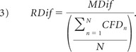
The difference in velocity magnitude and singular energy between CFD and 3D PC-MR imaging was determined for every voxel and subsequently averaged over space to yield a mean paired difference (MDif) at every cardiac phase:

where N is the number of voxels. Its significance was tested with a paired t test; P < .05 was considered statistically significantly different. The SD of the paired difference (SDif) was calculated as well A relative difference in velocity magnitude between both methods was based on the mean CFD velocity magnitude per subject:

graphic file with name zj400913-3484-m03.jpg

Differences in flow direction were calculated from the angle difference between corresponding velocity vectors. Because the distribution of the angle difference was not normal, median rather than mean values were calculated.

Results

The SNR of the 3D PC-MR imaging velocity measurements was 19.5 ± 3.4.

Figure 1 shows intra-aneurysmal flow patterns in 4 aneurysms. In systole, the circular motion in the vortices and the direction of inflow jets were qualitatively similar for the 3 methods. This finding can further be appreciated from the pathlines in Fig 2. In Fig 1 for diastole, the vortices of the 3D PC-MR imaging measurement appeared disrupted and irregular in most aneurysms.

Fig 1. — Velocity vector images in a characteristic section depicting the main vortex in 4 aneurysms and the inflow jet in 3 of the aneurysms. The images depict the aneurysms at peak systole and diastole in isosurfaces (gray) for 3D PC-MR imaging, CFD with inflow boundary conditions obtained from 2D PC-MR imaging, and CFD with inflow boundary conditions obtained from 3D PC-MR imaging.

Fig 2. — Pathlines over the entire cardiac cycle depicting similar complex flow in aneurysm volumes (gray background) of aneurysms 1, 4, 5, and 7 for 3D PC-MR imaging; CFD with inflow boundary conditions obtained from 2D PC-MR imaging; and CFD with inflow boundary conditions obtained from 3D PC-MR imaging.

For most aneurysms, the 3D PC-MR imaging measurements resulted in higher velocity magnitude values than CFD with inflow boundary conditions obtained from 2D PC-MR imaging (On-line Table 3). When inflow boundary conditions from 3D PC-MR imaging were used, the velocity magnitude values were higher for CFD than for 3D PC-MR imaging in a few simulations. For both CFD methods, the SDif and the RDif were higher in systole than in diastole and differences in estimated local flow direction were found primarily in diastole.

The Bland-Altman plots in On-line Figs 1–4 show similar behavior for the difference in velocity magnitude and singular energy between 3D PC-MR imaging and both CFD methods

In Fig 3, the locations with singular energy magnitude higher than half the maximum are displayed for 4 aneurysms. For aneurysms 1, 2, and 3, the locations and magnitudes of the maximum singular energy were similar. For aneurysm 5, the magnitude of the singular energy was approximately twice as low for both CFD methods. RDif averaged over all aneurysms in systole was a factor of 3 smaller for singular energy than for velocity magnitude (On-line Table 4). .

On-line Fig 5A shows that in systole an offset in velocity magnitude was found for the difference between 3D PC-MR imaging and CFD with 2D PC-MR imaging inflow boundary conditions. For velocity magnitude at diastole and singular energy at both systole and diastole, the Bland-Altman plots (On-line Figs 5 and 6) were similar for the difference between 3D PC-MR imaging and CFD with 2D PC-MR imaging and 3D PC-MR imaging inflow boundary conditions.

In On-line Table 2, MDif, SDif, and RDif are given for the separated inflow vessel and dome of the aneurysms. At systole, MDif was generally higher for the inflow region than for the dome, while RDif was lower for the inflow region than the dome. Further differences were similar to the analysis of the total geometry.

Discussion

Studies comparing 3D PC-MR imaging with CFD on a voxel-by-voxel basis in human aneurysms at 3T are not available in the literature, to our knowledge. One study compared 3D PC-MR imaging with CFD in the aorta,²⁸ and 1 study in 5 intracranial aneurysms at 1.5T at relatively low spatial resolution.²⁹ Another study compared 3D PC-MR imaging with CFD in canine aneurysm models.³⁰ All studies found a good qualitative agreement between both techniques and a moderate quantitative agreement. Note that the purpose of the CFD simulations in this study was to compare the results with the 3D PC-MR imaging measurements. To compare the modalities on a voxel basis, we downsized the flow fields obtained from CFD simulations to the voxel size of 3D PC-MR imaging. The original CFD data were therefore not displayed.

The need for reliable patient-specific CFD simulations has been described by many authors. However, the prescription of inflow boundary conditions that produce accurate CFD results is still a matter of debate. Several studies used flow rates that were measured with 2D PC-MR imaging in separate healthy volunteers.^9,31 Patient-specific spatial and temporal velocity vector values as measured with 3D PC-MR imaging at each node of the inflow boundary and subsequent comparison with 3D PC-MR imaging have been applied at relatively low resolution in only 2 studies.^28,29 This is the first study to perform this comparison in intracranial aneurysms at 3T, to our knowledge.

To be able to prescribe boundary conditions with high spatial and temporal resolution, we performed a 2D PC-MR imaging measurement to obtain inflow profiles. Furthermore, the difference with inflow boundary conditions obtained at lower spatial and temporal resolution was investigated by prescribing inflow boundary conditions obtained from 3D PC-MR imaging. It was shown that different inflow boundary conditions produce different results in terms of velocity magnitude. However, the differences in the direction of the velocity vectors, expressed as the angle between vortices or as locations of vortices by singular energy, were found to be small when using inflow boundary conditions obtained from different techniques.

On average, the 3D PC-MR imaging measurements resulted in 30% higher flow estimates than the 2D PC-MR imaging ones. Discrepancies between flow measurements from 2D and 3D PC-MR imaging (±18%)³² or 2D and endovascular sonography (±15%)³³ have been reported in the literature earlier. Wentland et al³⁴ concluded that flow measurements in healthy volunteers in the renal vasculature revealed that 3D measurements tended to be more internally consistent than 2D measurements.

In On-line Table 1, it can be seen that segmentation of the sections obtained by 3D PC-MR imaging resulted in larger areas than for the 2D PC-MR imaging sections. A slightly smaller segmentation can result in the discarding of many voxels around the circumference of the vessel and therefore in severe area underestimation. Despite the lower mean velocities in the 3D PC-MR imaging measurement, the larger vessel area resulted in larger flow values than 2D PC-MR imaging.

A consequence of the smaller vessel segmentation in 2D PC-MR imaging was that velocities at nodes at the edges of the inflow boundary in CFD were interpolated toward zero. The wider segmentation in 3D PC-MR imaging led to higher input velocities at the edges of the inflow boundary in the CFD simulation. Therefore 3D PC-MR imaging corresponded better with CFD simulations with inflow boundary conditions obtained from 3D PC-MR imaging than the simulations by using inflow boundary conditions obtained from 2D PC-MR imaging.

Six simulations with boundary conditions obtained from 3D PC-MR imaging were performed; in 2 cases, the inflow of the CFD was located outside the imaging volume of the PC-MR imaging sequence.

The systematic differences in local velocity were reduced 5-fold for MDif and 2-fold for RDif by using inflow boundary conditions from 3D PC-MR imaging instead of 2D PC-MR imaging. The fan-shaped profiles of the Bland-Altman plots in On-line Figs 1–4 reveal that the discrepancies between 3D-PC-MR imaging and both CFD methods are proportional with the mean of 3D PC-MR imaging and CFD. Random differences (SDif) were similar for both inflow boundary conditions. The results for the singular energy and the median angle were similar. We therefore conclude that different inflow boundary conditions have a large influence on magnitude of velocity values. However, velocity vector directions and locations and magnitude of vortices are fairly independent of inflow boundary conditions.

The singular energy measure as presented in this study is introduced to facilitate the comparison between 3D PC-MR imaging and CFD. Singular energy provides a quantitative measure of flow patterns. It is unclear whether it may lead to more insight into the nature of the aneurysm with respect to rupture, as has been discussed in the literature recently.^35,36 While this is an intriguing possibility, it was not the purpose of the current work to address the predictive value of this quantity.

Another limitation is the semiautomatic segmentation of the 3D rotational angiography dataset, resulting in possible under- or overestimation of neck width.³⁷ Also limitations with regard to the 3D PC-MR imaging setup may contribute to the found discrepancies between both techniques. In our study, SNR values within aneurysms were relatively low due to small voxel sizes and the use of parallel imaging.³⁸ Therefore, at low velocities during diastole, the velocity may be overestimated due to noise. Furthermore, the temporal resolution of the 3D PC-MR imaging was relatively low, resulting in temporal low-pass filtering (ie, underestimation of velocities in the systolic phase).

It is clear that more accurate estimation of intracranial aneurysm hemodynamics from PC-MR imaging requires improved technology. Higher field strengths can improve SNR.³⁹ One recently developed promising technique to improve PC-MR imaging measurement is divergence-reduction processing.⁴⁰

Conclusions

In this study, high-resolution 3D PC-MR imaging was compared with patient-specific CFD on a voxel-by-voxel basis in 8 aneurysms. In peak systole, qualitative similarities in flow features such as vortical flow patterns and inflow behavior were evident. In end diastole, the flow patterns of the 3D PC-MR imaging measurements were different compared with those generated with CFD due to the low velocity-to-noise ratio of the 3D PC-MR imaging measurements. Singular energy calculation revealed quantitative agreement between 3D PC-MR imaging and CFD in systole.

Supplementary Material

3484_materials.pdf

3484_materials.pdf^{(7.3MB, pdf)}

ABBREVIATIONS:

CFD: computational fluid dynamics
PC-MRI: cine phase-contrast MR imaging
RA: rotational angiography
VNR: velocity-to noise ratio

Footnotes

Disclosures: Pim van Ooij—RELATED: Grant: Nuts Ohra Foundation (the Netherlands).* Joppe J. Schneiders—RELATED: Grant: Nuts Ohra research grant,* Comments: to investigate the role of intra-aneurysmal hemodynamics in rupture-risk assessment. Charles B. Majoie—RELATED: Grant: Nuts Ohra Foundation,* UNRELATED: Grants/Grants Pending: Netherlands Heart Foundation.* *Money paid to the institution.

This work was supported by a grant from the Nuts Ohra Foundation, the Netherlands, a research grant for research into the role of hemodynamics in the rupture risk assessment of intracranial aneurysms.

REFERENCES

1.Nieuwkamp DJ, Setz LE, Algra A, et al. Changes in case fatality of aneurysmal subarachnoid haemorrhage over time, according to age, sex, and region: a meta-analysis. Lancet Neurol 2009;8:635–42 [DOI] [PubMed] [Google Scholar]
2.Greebe P, Rinkel GJ, Hop JW, et al. Functional outcome and quality of life 5 and 12.5 years after aneurysmal subarachnoid haemorrhage. J Neurol 2010;257:2059–64 [DOI] [PMC free article] [PubMed] [Google Scholar]
3.Vega C, Kwoon JV, Lavine SD. Intracranial aneurysms: current evidence and clinical practice. Am Fam Physician 2002;66:601–08 [PubMed] [Google Scholar]
4.Wiebers DO, Whisnant JP, Huston J, 3rd, et al. Unruptured intracranial aneurysms: natural history, clinical outcome, and risks of surgical and endovascular treatment. Lancet 2003;362:103–10 [DOI] [PubMed] [Google Scholar]
5.Ford MD, Nikolov HN, Milner JS, et al. PIV-measured versus CFD-predicted flow dynamics in anatomically realistic cerebral aneurysm models. J Biomech Eng 2008;130:021015 [DOI] [PubMed] [Google Scholar]
6.Geers AJ, Larrabide I, Radaelli AG, et al. Patient-specific computational hemodynamics of intracranial aneurysms from 3D rotational angiography and CT angiography: an in vivo reproducibility study. AJNR Am J Neuroradiol 2011;32:581–86 [DOI] [PMC free article] [PubMed] [Google Scholar]
7.Ford MD, Lee SW, Lownie SP, et al. On the effect of parent-aneurysm angle on flow patterns in basilar tip aneurysms: towards a surrogate geometric marker of intra-aneurismal hemodynamics. J Biomech 2008;41:241–48 [DOI] [PubMed] [Google Scholar]
8.Rayz VL, Boussel L, Lawton MT, et al. Numerical modeling of the flow in intracranial aneurysms: prediction of regions prone to thrombus formation. Ann Biomed Eng 2008;36:1793–1804 [DOI] [PMC free article] [PubMed] [Google Scholar]
9.Cebral JR, Castro MA, Burgess JE, et al. Characterization of cerebral aneurysms for assessing risk of rupture by using patient-specific computational hemodynamics models. AJNR Am J Neuroradiol 2005;26:2550–59 [PMC free article] [PubMed] [Google Scholar]
10.Boussel L, Rayz V, Martin A, et al. Phase-contrast magnetic resonance imaging measurements in intracranial aneurysms in vivo of flow patterns, velocity fields, and wall shear stress: comparison with computational fluid dynamics. Magn Reson Med 2009;61:409–17 [DOI] [PMC free article] [PubMed] [Google Scholar]
11.Cebral JR, Castro MA, Appanaboyina S, et al. Efficient pipeline for image-based patient-specific analysis of cerebral aneurysm hemodynamics: technique and sensitivity. IEEE Trans Med Imaging 2005;24:457–67 [DOI] [PubMed] [Google Scholar]
12.Chien A, Castro MA, Tateshima S, et al. Quantitative hemodynamic analysis of brain aneurysms at different locations. AJNR AM J Neuroradiol 2009;30:1507–12 [DOI] [PMC free article] [PubMed] [Google Scholar]
13.Sforza DM, Putman CM, Cebral JR. Hemodynamics of cerebral aneurysms. Annu Rev Fluid Mech 2009;41:91–107 [DOI] [PMC free article] [PubMed] [Google Scholar]
14.Venugopal P, Valentino D, Schmitt H, et al. Sensitivity of patient-specific numerical simulation of cerebral aneurysm hemodynamics to inflow boundary conditions. J Neurosurg 2007;106:1051–60 [DOI] [PubMed] [Google Scholar]
15.Mut F, Lohner R, Chien A, et al. Computational hemodynamics framework for the analysis of cerebral aneurysms. Int J Numer Method Biomed Eng 2011;27:822–39 [DOI] [PMC free article] [PubMed] [Google Scholar]
16.van Ooij P, Guédon A, Poelma C, et al. Complex flow patterns in a real-size intracranial aneurysm phantom: phase contrast MRI compared with particle image velocimetry and computational fluid dynamics. NMR in Biomed 2012;25:14–26 [DOI] [PubMed] [Google Scholar]
17.Wilson JT, Pettigrew LE, Teasdale GM. Structured interviews for the Glasgow Outcome Scale and the extended Glasgow Outcome Scale: guidelines for their use. J Neurotrauma 1998;15:573–85 [DOI] [PubMed] [Google Scholar]
18.Slavin GS, Bluemke DA. Spatial and temporal resolution in cardiovascular MR imaging: review and recommendations. Radiology 2005;234:330–38 [DOI] [PubMed] [Google Scholar]
19.Lotz J, Meier C, Leppert A, et al. Cardiovascular flow measurement with phase-contrast MR imaging: basic facts and implementation. Radiographics 2002;22:651–71 [DOI] [PubMed] [Google Scholar]
20.Li C, Xu C, Gui C, et al. Level set evolution without re-initialization: a new variational formulation. In: Proceedings of the 2005 IEEE Computer Society Conference on Computer Vision and Pattern Recognition, San Diego, California. June 20–25, 2005:430–36 [Google Scholar]
21.Antiga L, Piccinelli M, Botti L, et al. An image-based modeling framework for patient-specific computational hemodynamics. Med Biol Eng Comput 2008;46:1097–112 [DOI] [PubMed] [Google Scholar]
22.Jenkinson M, Smith S. A global optimisation method for robust affine registration of brain images. Med Image Anal 2001;5:143–56 [DOI] [PubMed] [Google Scholar]
23.Murray CD. The physiological principle of minimum work: I. The vascular system and the cost of blood volume. Proc Natl Acad Sci U S A 1926;12:207–14 [DOI] [PMC free article] [PubMed] [Google Scholar]
24.Price RR, Axel L, Morgan T, et al. Quality assurance methods and phantoms for magnetic resonance imaging: report of AAPM Nuclear Magnetic Resonance Task Group No. 1. Med Phys 1990;17:287–95 [DOI] [PubMed] [Google Scholar]
25.Liu W, Ribeiro E. Scale and rotation invariant detection of singular patterns in vector flow fields. In: Hancock E, Wilson R, Windeatt T, et al., eds. SSPR & SPR Proceedings of the 2010 Joint IAPR International Conference on Structural, Syntactic, and Statistical Pattern Recognition, LNCS No, 6218. Berlin: Springer-Verlag; 2010:522–31 [Google Scholar]
26.Marquering HA, van Ooij P, Streekstra GJ, et al. Multiscale flow patterns within an intracranial aneurysm phantom. IEEE Trans Biomed Eng 2011;58:3447–50 [DOI] [PubMed] [Google Scholar]
27.Cebral JR, Mut F, Weir J, et al. Association of hemodynamic characteristics and cerebral aneurysm rupture. AJNR Am J Neuroradiol 2011;32:264–70 [DOI] [PMC free article] [PubMed] [Google Scholar]
28.Stalder AF, Liu Z, Hennig J, et al. Patient specific hemodynamics: combined 4D flow-sensitive MRI and CFD. In: Wittek A, Nielsen PMF, Miller K, eds. Computational Biomechanics for Medicine. New York: Springer-Verlag; 2011:27–38 [Google Scholar]
29.Isoda H, Ohkura Y, Kosugi T, et al. Comparison of hemodynamics of intracranial aneurysms between MR fluid dynamics using 3D cine phase-contrast MRI and MR-based computational fluid dynamics. Neuroradiology 2010;52:913–20 [DOI] [PMC free article] [PubMed] [Google Scholar]
30.Jiang J, Johnson K, Valen-Sendstad K, et al. Flow characteristics in a canine aneurysm model: a comparison of 4D accelerated phase-contrast MR measurements and computational fluid dynamics simulations. Med Phys 2011;38:6300–12 [DOI] [PMC free article] [PubMed] [Google Scholar]
31.Castro MA, Putman CM, Cebral JR. Computational fluid dynamics modeling of intracranial aneurysms: effects of parent artery segmentation on intra-aneurysmal hemodynamics. AJNR Am J Neuroradiol 2006;27:1703–09 [PMC free article] [PubMed] [Google Scholar]
32.Stalder A, Russe M, Frydrychowicz A, et al. Quantitative 2D and 3D phase contrast MRI: optimized analysis of blood flow and vessel wall parameters. Magn Reson Med 2008;60:1218–31 [DOI] [PubMed] [Google Scholar]
33.Schneiders JJ, Ferns SP, van Ooij P, et al. Comparison of phase-contrast MR imaging and endovascular sonography for intracranial blood flow velocity measurements. AJNR Am J Neuroradiol 2012;33:1786–90 [DOI] [PMC free article] [PubMed] [Google Scholar]
34.Wentland A, Grist TM, Wieben O. Repeatability and internal consistency of abdominal 2D and 4D PC MR flow measurements. J Cardiovasc Magn Reson 2012;14(Suppl 1):W13. [DOI] [PMC free article] [PubMed] [Google Scholar]
35.Kallmes DF. Point: CFD—computational fluid dynamics or confounding factor dissemination. AJNR Am J Neuroradiol 2012;33:395–96 [DOI] [PMC free article] [PubMed] [Google Scholar]
36.Cebral JR, Meng H. Counterpoint: realizing the clinical utility of computational fluid dynamics–closing the gap. AJNR Am J Neuroradiol 2012;33:396–98 [DOI] [PMC free article] [PubMed] [Google Scholar]
37.Schneiders JJ, Marquering HA, Antiga L, et al. Intracranial aneurysm neck size overestimation with 3D rotational angiography: an exploratory study on the impact on intra-aneurysmal hemodynamics simulated with computational fluid dynamics. AJNR Am J Neuroradiol 2013;34:121–28 [DOI] [PMC free article] [PubMed] [Google Scholar]
38.Thunberg P, Karlsson M, Wigstrom L. Accuracy and reproducibility in phase contrast imaging using SENSE. Magn Reson Med 2003;50:1061–68 [DOI] [PubMed] [Google Scholar]
39.van Ooij P, Zwanenburg JJM, Visser F, et al. Quantification and visualization of flow in the circle of Willis: time-resolved three-dimensional phase contrast MRI at 7 T compared with 3 T. Magn Reson Med 2013;69:868–76 [DOI] [PubMed] [Google Scholar]
40.Busch J, Giese D, Wissmann L, et al. Construction of divergence-free velocity fields from cine 3D phase-contrast flow measurements. Magn Reson Med 2013;69:200–10 [DOI] [PubMed] [Google Scholar]

Associated Data

This section collects any data citations, data availability statements, or supplementary materials included in this article.

Supplementary Materials

3484_materials.pdf

3484_materials.pdf^{(7.3MB, pdf)}

[B1] 1.Nieuwkamp DJ, Setz LE, Algra A, et al. Changes in case fatality of aneurysmal subarachnoid haemorrhage over time, according to age, sex, and region: a meta-analysis. Lancet Neurol 2009;8:635–42 [DOI] [PubMed] [Google Scholar]

[B2] 2.Greebe P, Rinkel GJ, Hop JW, et al. Functional outcome and quality of life 5 and 12.5 years after aneurysmal subarachnoid haemorrhage. J Neurol 2010;257:2059–64 [DOI] [PMC free article] [PubMed] [Google Scholar]

[B3] 3.Vega C, Kwoon JV, Lavine SD. Intracranial aneurysms: current evidence and clinical practice. Am Fam Physician 2002;66:601–08 [PubMed] [Google Scholar]

[B4] 4.Wiebers DO, Whisnant JP, Huston J, 3rd, et al. Unruptured intracranial aneurysms: natural history, clinical outcome, and risks of surgical and endovascular treatment. Lancet 2003;362:103–10 [DOI] [PubMed] [Google Scholar]

[B5] 5.Ford MD, Nikolov HN, Milner JS, et al. PIV-measured versus CFD-predicted flow dynamics in anatomically realistic cerebral aneurysm models. J Biomech Eng 2008;130:021015 [DOI] [PubMed] [Google Scholar]

[B6] 6.Geers AJ, Larrabide I, Radaelli AG, et al. Patient-specific computational hemodynamics of intracranial aneurysms from 3D rotational angiography and CT angiography: an in vivo reproducibility study. AJNR Am J Neuroradiol 2011;32:581–86 [DOI] [PMC free article] [PubMed] [Google Scholar]

[B7] 7.Ford MD, Lee SW, Lownie SP, et al. On the effect of parent-aneurysm angle on flow patterns in basilar tip aneurysms: towards a surrogate geometric marker of intra-aneurismal hemodynamics. J Biomech 2008;41:241–48 [DOI] [PubMed] [Google Scholar]

[B8] 8.Rayz VL, Boussel L, Lawton MT, et al. Numerical modeling of the flow in intracranial aneurysms: prediction of regions prone to thrombus formation. Ann Biomed Eng 2008;36:1793–1804 [DOI] [PMC free article] [PubMed] [Google Scholar]

[B9] 9.Cebral JR, Castro MA, Burgess JE, et al. Characterization of cerebral aneurysms for assessing risk of rupture by using patient-specific computational hemodynamics models. AJNR Am J Neuroradiol 2005;26:2550–59 [PMC free article] [PubMed] [Google Scholar]

[B10] 10.Boussel L, Rayz V, Martin A, et al. Phase-contrast magnetic resonance imaging measurements in intracranial aneurysms in vivo of flow patterns, velocity fields, and wall shear stress: comparison with computational fluid dynamics. Magn Reson Med 2009;61:409–17 [DOI] [PMC free article] [PubMed] [Google Scholar]

[B11] 11.Cebral JR, Castro MA, Appanaboyina S, et al. Efficient pipeline for image-based patient-specific analysis of cerebral aneurysm hemodynamics: technique and sensitivity. IEEE Trans Med Imaging 2005;24:457–67 [DOI] [PubMed] [Google Scholar]

[B12] 12.Chien A, Castro MA, Tateshima S, et al. Quantitative hemodynamic analysis of brain aneurysms at different locations. AJNR AM J Neuroradiol 2009;30:1507–12 [DOI] [PMC free article] [PubMed] [Google Scholar]

[B13] 13.Sforza DM, Putman CM, Cebral JR. Hemodynamics of cerebral aneurysms. Annu Rev Fluid Mech 2009;41:91–107 [DOI] [PMC free article] [PubMed] [Google Scholar]

[B14] 14.Venugopal P, Valentino D, Schmitt H, et al. Sensitivity of patient-specific numerical simulation of cerebral aneurysm hemodynamics to inflow boundary conditions. J Neurosurg 2007;106:1051–60 [DOI] [PubMed] [Google Scholar]

[B15] 15.Mut F, Lohner R, Chien A, et al. Computational hemodynamics framework for the analysis of cerebral aneurysms. Int J Numer Method Biomed Eng 2011;27:822–39 [DOI] [PMC free article] [PubMed] [Google Scholar]

[B16] 16.van Ooij P, Guédon A, Poelma C, et al. Complex flow patterns in a real-size intracranial aneurysm phantom: phase contrast MRI compared with particle image velocimetry and computational fluid dynamics. NMR in Biomed 2012;25:14–26 [DOI] [PubMed] [Google Scholar]

[B17] 17.Wilson JT, Pettigrew LE, Teasdale GM. Structured interviews for the Glasgow Outcome Scale and the extended Glasgow Outcome Scale: guidelines for their use. J Neurotrauma 1998;15:573–85 [DOI] [PubMed] [Google Scholar]

[B18] 18.Slavin GS, Bluemke DA. Spatial and temporal resolution in cardiovascular MR imaging: review and recommendations. Radiology 2005;234:330–38 [DOI] [PubMed] [Google Scholar]

[B19] 19.Lotz J, Meier C, Leppert A, et al. Cardiovascular flow measurement with phase-contrast MR imaging: basic facts and implementation. Radiographics 2002;22:651–71 [DOI] [PubMed] [Google Scholar]

[B20] 20.Li C, Xu C, Gui C, et al. Level set evolution without re-initialization: a new variational formulation. In: Proceedings of the 2005 IEEE Computer Society Conference on Computer Vision and Pattern Recognition, San Diego, California. June 20–25, 2005:430–36 [Google Scholar]

[B21] 21.Antiga L, Piccinelli M, Botti L, et al. An image-based modeling framework for patient-specific computational hemodynamics. Med Biol Eng Comput 2008;46:1097–112 [DOI] [PubMed] [Google Scholar]

[B22] 22.Jenkinson M, Smith S. A global optimisation method for robust affine registration of brain images. Med Image Anal 2001;5:143–56 [DOI] [PubMed] [Google Scholar]

[B23] 23.Murray CD. The physiological principle of minimum work: I. The vascular system and the cost of blood volume. Proc Natl Acad Sci U S A 1926;12:207–14 [DOI] [PMC free article] [PubMed] [Google Scholar]

[B24] 24.Price RR, Axel L, Morgan T, et al. Quality assurance methods and phantoms for magnetic resonance imaging: report of AAPM Nuclear Magnetic Resonance Task Group No. 1. Med Phys 1990;17:287–95 [DOI] [PubMed] [Google Scholar]

[B25] 25.Liu W, Ribeiro E. Scale and rotation invariant detection of singular patterns in vector flow fields. In: Hancock E, Wilson R, Windeatt T, et al., eds. SSPR & SPR Proceedings of the 2010 Joint IAPR International Conference on Structural, Syntactic, and Statistical Pattern Recognition, LNCS No, 6218. Berlin: Springer-Verlag; 2010:522–31 [Google Scholar]

[B26] 26.Marquering HA, van Ooij P, Streekstra GJ, et al. Multiscale flow patterns within an intracranial aneurysm phantom. IEEE Trans Biomed Eng 2011;58:3447–50 [DOI] [PubMed] [Google Scholar]

[B27] 27.Cebral JR, Mut F, Weir J, et al. Association of hemodynamic characteristics and cerebral aneurysm rupture. AJNR Am J Neuroradiol 2011;32:264–70 [DOI] [PMC free article] [PubMed] [Google Scholar]

[B28] 28.Stalder AF, Liu Z, Hennig J, et al. Patient specific hemodynamics: combined 4D flow-sensitive MRI and CFD. In: Wittek A, Nielsen PMF, Miller K, eds. Computational Biomechanics for Medicine. New York: Springer-Verlag; 2011:27–38 [Google Scholar]

[B29] 29.Isoda H, Ohkura Y, Kosugi T, et al. Comparison of hemodynamics of intracranial aneurysms between MR fluid dynamics using 3D cine phase-contrast MRI and MR-based computational fluid dynamics. Neuroradiology 2010;52:913–20 [DOI] [PMC free article] [PubMed] [Google Scholar]

[B30] 30.Jiang J, Johnson K, Valen-Sendstad K, et al. Flow characteristics in a canine aneurysm model: a comparison of 4D accelerated phase-contrast MR measurements and computational fluid dynamics simulations. Med Phys 2011;38:6300–12 [DOI] [PMC free article] [PubMed] [Google Scholar]

[B31] 31.Castro MA, Putman CM, Cebral JR. Computational fluid dynamics modeling of intracranial aneurysms: effects of parent artery segmentation on intra-aneurysmal hemodynamics. AJNR Am J Neuroradiol 2006;27:1703–09 [PMC free article] [PubMed] [Google Scholar]

[B32] 32.Stalder A, Russe M, Frydrychowicz A, et al. Quantitative 2D and 3D phase contrast MRI: optimized analysis of blood flow and vessel wall parameters. Magn Reson Med 2008;60:1218–31 [DOI] [PubMed] [Google Scholar]

[B33] 33.Schneiders JJ, Ferns SP, van Ooij P, et al. Comparison of phase-contrast MR imaging and endovascular sonography for intracranial blood flow velocity measurements. AJNR Am J Neuroradiol 2012;33:1786–90 [DOI] [PMC free article] [PubMed] [Google Scholar]

[B34] 34.Wentland A, Grist TM, Wieben O. Repeatability and internal consistency of abdominal 2D and 4D PC MR flow measurements. J Cardiovasc Magn Reson 2012;14(Suppl 1):W13. [DOI] [PMC free article] [PubMed] [Google Scholar]

[B35] 35.Kallmes DF. Point: CFD—computational fluid dynamics or confounding factor dissemination. AJNR Am J Neuroradiol 2012;33:395–96 [DOI] [PMC free article] [PubMed] [Google Scholar]

[B36] 36.Cebral JR, Meng H. Counterpoint: realizing the clinical utility of computational fluid dynamics–closing the gap. AJNR Am J Neuroradiol 2012;33:396–98 [DOI] [PMC free article] [PubMed] [Google Scholar]

[B37] 37.Schneiders JJ, Marquering HA, Antiga L, et al. Intracranial aneurysm neck size overestimation with 3D rotational angiography: an exploratory study on the impact on intra-aneurysmal hemodynamics simulated with computational fluid dynamics. AJNR Am J Neuroradiol 2013;34:121–28 [DOI] [PMC free article] [PubMed] [Google Scholar]

[B38] 38.Thunberg P, Karlsson M, Wigstrom L. Accuracy and reproducibility in phase contrast imaging using SENSE. Magn Reson Med 2003;50:1061–68 [DOI] [PubMed] [Google Scholar]

[B39] 39.van Ooij P, Zwanenburg JJM, Visser F, et al. Quantification and visualization of flow in the circle of Willis: time-resolved three-dimensional phase contrast MRI at 7 T compared with 3 T. Magn Reson Med 2013;69:868–76 [DOI] [PubMed] [Google Scholar]

[B40] 40.Busch J, Giese D, Wissmann L, et al. Construction of divergence-free velocity fields from cine 3D phase-contrast flow measurements. Magn Reson Med 2013;69:200–10 [DOI] [PubMed] [Google Scholar]

PERMALINK

3D Cine Phase-Contrast MRI at 3T in Intracranial Aneurysms Compared with Patient-Specific Computational Fluid Dynamics

P van Ooij

JJ Schneiders

HA Marquering

CB Majoie

E van Bavel

AJ Nederveen