Non-Linear Image Distortions in Flexible Fiberoptic Endoscopes and their Effects on Calibrated Horizontal Measurements Using High-Speed Videoendoscopy

Summary:

Laryngeal images obtained via high-speed videoendoscopy are an invaluable source of information for the advancement of voice science because they can capture the true cycle-to-cycle vibratory characteristics of the vocal folds in addition to the transient behaviors of the phonatory mechanism, such as onset, offset, and breaks. This information is obtained through relating the spatial and temporal features from acquired images using objective measurements or subjective assessments. While these images are calibrated temporally, a great challenge is the lack of spatial calibration. Recently, a laser-projection system allowing for spatial calibration was developed. However, various sources of optical distortions deviate the images from reflecting the reality. The main purpose of this study was to evaluate the effect of the fiberoptic flexible endoscope distortions on the calibration of images acquired by the laser-projection system. Specifically, it is shown that two sources of nonlinear distortions could deviate captured images from reality. The first distortion stems from the wide-angle lens used in flexible endoscopes. It is shown that endoscopic images have a significantly higher spatial resolution in the center of the field of view than in its periphery. The difference between the two could lead to as high as 26.4% error in calibrated horizontal measurements. The second distortion stems from variation in the imaging angle. It is shown that the disparity between spatial resolution in the center and periphery of endoscopic images increases as the imaging angle deviates from the perpendicular position. Furthermore, it is shown that when the imaging angle varies, the symmetry of the distortion is also affected significantly. The combined distortions could lead to calibrated horizontal measurement errors as high as 65.7%. The implications of the findings on objective measurements and subjective visual assessments are discussed. These findings can contribute to the refinement of the methods for clinical assessment of voice disorders. Considering that the studied phenomena are due to optical principles, the findings of this study, especially those related to the effects of the imaging angle, can provide further insights regarding other endoscopic instruments (eg, distal-chip and rigid endoscopes) and procedures (eg, gastroendoscopy and colonoscopy).

INTRODUCTION

Imaging techniques provide a direct method for observation, assessment and precision measurement of characteristics of the laryngeal mechanisms. Therefore, they are important in voice research^1,2 and functional assessment of voice production.^3–5 Videostroboscopy, high-speed videoendoscopy (HSV), and videokymography are the main imaging modalities for acquiring optical images from the laryngeal behavior. Videostroboscopy can provide a real-time and audio-synchronized “slow-motion” effect of the vibration of the vocal fold. Additionally, distal-chip videostroboscopy systems can provide higher quality images. Therefore, videostroboscopy is considered the “gold standard” in clinical applications.^5–7 However, consecutive frames of videostroboscopy are taken from different vibratory cycles. This leads to several limitations regarding its applicability. Specifically, the intra-cycle kinematics of the phonatory mechanism (eg, velocity, phase symmetry, and periodicity) cannot be measured. Additionally, videostroboscopy requires triggering that depends on estimating the vibratory phase of the vocal folds from an external signal. It means that, videostroboscopy can only be used for observation of quasi-periodic phenomena, while transient behaviors (eg, voice onset, offset, breaks, and aperiodicity) cannot be studied using videostroboscopy. Finally, if vibratory phases are estimated inaccurately (eg, irregular or aperiodic vibration), the assembled “slow-motion” images would substantially deviate from the true pattern.^7,8 Conversely, HSV can capture the true vibratory behavior of the vocal folds and therefore it can be used for studying transient phenomena, as well as, irregular and aperiodic vibration of the vocal folds. However, distal-chip technology cannot be applied to HSV due to significant technological limitations. It is unforeseeable for these limitations to be resolved in the near future, thus flexible HSV is limited to the use of fiberoptic technology. Finally, considering the recent advancements using laser-calibrated fiberoptic HSV systems^9,10, the kinematics, and biomechanics of the phonatory mechanism can be studied more accurately.

Regardless of the imaging modality (eg, videostroboscopy, HSV, or videokymography) the acquired images can be evaluated using two main approaches of visual-perceptual assessments¹ or image measurements. Visual-perceptual assessments and image measurements respectively lead to subjective and objective evaluations of some features of the phonatory mechanism. Using a different taxonomy, features from the acquired images may belong to spatial, temporal, or spatial-temporal domains. Some examples of spatial features would be the size of a lesion,¹¹ glottal closure pattern,¹² and glottic angle.¹³ Some examples of spatial-temporal features would be velocity measurements,^14,15 mucosal wave,¹⁶ glottal area waveform,^17,18 and kymogram.^19,20 Objective measurements and subjective assessments based on spatial and spatial-temporal features rely on some implicit but important assumptions. Those implicit assumptions may vary depending on the purpose of measurements or assessments. For example, the percentage change in the pixel length (ie, the uncalibrated length in the image) of a lesion pre- and post-intervention could be used as a direct evaluation criterion for measuring and comparing the efficacy of different interventions. In this group-comparison scenario, an implicit assumption is that for each subject the measurement from the pre and post conditions are on the same scale, and hence can be compared with each other. Being on the same scale means that if pixel length of the lesion in the postintervention image is reduced by 20%, in reality, the actual absolute length in mm (ie, the calibrated length) of that lesion has also been reduced by 20%. More precisely, the implicit assumption is that the mm size of a pixel (ie, pixel size) in the pre and post conditions for each subject are the same. We call this a within-subject size comparison assumption. It is noteworthy that most image-based group comparison research in voice (both objective and subjective) is based on this assumption. The importance of this assumption has been noted at least in one study, where authors explicitly accounted for possible variations between pixel sizes in pre and post conditions.¹¹ On the other hand, if the purpose of the research is to compare different groups or to relate post-intervention changes in the lesion size to some outcomes of the phonatory mechanisms (eg, acoustic measurements), a more strict assumption should hold. More precisely, not only the mm size of pixels in the pre- and post-conditions for each subject should be the same, but also the mm size of pixels in different subjects should be the same. We call this a between-subject size comparison assumption. This implicit assumption is made in most (if not all) image-based regression and other modeling studies in voice. It is noteworthy that the between-subject size comparison assumption satisfies the within-subject size comparison assumption; however, the other direction does not necessarily hold.

Different approaches are possible to satisfy the between-subject size comparison assumption. Regardless of the employed approach, all methods are based on the same principle. Basically, pixels are building blocks of images. Therefore, if we know the mm size of pixels, all objects in the image could be mapped in mm scale which is a universal and standard basis. Intraoperative calibrated images^8,21 and laser-calibrated imaging systems^10,22–24 are some possible approaches for determining the mm size of pixels. In the intraoperative calibration method, a surgical instrument is placed next to a target tissue and an image is recorded.^8,21 Considering the known mm length of the surgical instrument, the mm size of pixels in the image could be estimated. On the other hand, laser-calibrated systems are based on well-designed laser patterns that are projected on the laryngeal tissues. The laser patterns often have specific topological characteristics that help with determining the mm size of pixels in the acquired images. Parallel-laser projection methods are among the easiest approach for deriving the mm size of pixels in this category. In parallel-laser projection systems, the information for determining the mm size of a pixel in the acquired images comes from the known mm distance between parallel laser beams. Ghasemzadeh et al.⁹ has presented a summary of existing laser-based methods and the interested reader may refer to it.

Deriving the mm size of pixels based on intraoperative calibrated images or parallel laser projection is based on an important condition. Basically in these approaches, the mm size of a pixel is computed from some specific part of the image−−in intraoperative approach this is the target tissue that the surgical instrument is placed next to, and in laser projection is the part of the image that falls between two laser points−−and then we assume that the same number is valid for other parts of the image too. Specifically, we assume that all pixels in the image have the same mm sizes and therefore the conversion from pixel to mm can be achieved using a constant number (ie, independent from the spatial location of the pixel). This assumption is critical for both within-subject and between-subject size comparison applications, and its violation could lead to significant error in the measurements. To put this argument into perspective let us consider a hypothetical imaging system with a specific nonlinear distortion where pixels in the right half of the image correspond to 1 mm, and pixels in the left half of the image correspond to 0.5 mm. Obviously, using a constant pixel size would lead to significant errors in between-subject size comparison applications, as well as, within-subject size comparison applications (eg, if the lesion site in pre- and post-intervention are on different halves of the image). Based on this rationale the main aims of this research are to investigate if such nonlinear distortions are possible in flexible HSV endoscopy and if so, to quantify their impacts on subsequent horizontal measurements. To pursue these aims two research questions have been formed.

Q1: How much the mm size of a pixel depends on its spatial location?

Q2: How much the imaging angle affects the mm size of a pixel?

Reviewing the literature showed that the effect of nonlinear distortions has found little attention in the field. Hibi et al.²⁵ investigated the effects of nonlinear distortions in flexible endoscopes. They showed that the magnitude of distortion increases with the deviation of the imaging axis from the perpendicular angle.²⁵ Distortion as high as 20% was reported for a 30° deviation in the imaging angle. Considering that calibrated horizontal measurements were not possible at that time, that work was geared more toward practical recommendations for keeping the effect of distortions to a minimum. A different research aimed at studying the normative values of the glottic angle using flexible endoscopy acknowledged the significant effect of nonlinear barrel distortion on the measurements.¹³ However, the study neither provided details on how the distortion was compensated for, nor reported the magnitude of errors in presence of the nonlinear barrel distortion. Finally, a very recent work investigated the effects of parameters of HSV recordings on the estimation of the phonatory parameters of synthetic vocal folds.²⁶ This work suggested that the imaging angle was the most influential factor, where a 10° change in the imaging angle led to a 10% error in the estimation of the subglottal air pressure from the glottal area waveform.²⁶ However, none of these works were aimed at calibrated horizontal measurement and effects of barrel distortion or changes in the imaging angle on it.

The outcomes of this research could help us to better understand possible confounding factors in subjective assessments and objective measurements from flexible endoscopy images. Also, the outcomes will help us develop a more accurate and reliable method for horizontal calibration and measurements from a recently developed laser-calibrated flexible fiberoptic endoscope.¹⁰ It is expected for the derived horizontal measurement to improve our understanding from the effect of individual differences on the function of the phonatory mechanism²⁷ and consequently advancement of personalized medicine in the field of laryngology and speech language pathology. It is noteworthy that application of the outcomes is not limited to horizontal measurements from laser-calibrated endoscopes. For example, the outcomes could be utilized to increase accuracy of horizontal measurements from intraoperative images, as well as, any other calibration approach. Additionally, the outcomes of this research would shed light on possible confounding factors affecting accuracy and reliability of objective measurements and subjective evaluations on images recorded using distal-chip flexible endoscopes or rigid endoscopes. However, the exact effects for distal-chip flexible endoscopes and rigid endoscopes are not the purpose of this study and need to be investigated in a separate study. The rest of this paper is organized as follows. First, some relevant principles and background from optics are presented. The Material and Method section describes the experimental settings, as well as, details of the algorithms used in this study. The Experiments and Results section presents outcomes of the experiments followed by their interpretations and some relevant discussions. The results of the experiments are put into the bigger context in the Discussions section, where more general implications of this work are presented. Finally, the conclusions are drawn.

OPTICAL PRINCIPLES OF IMAGE FORMATION

The formation of an image in a camera follows principles of optics. Snell’s law is one of the main principles that govern image formation in the presence of a lens.²⁸ Based on Snell’s law, the path of a ray of light changes, when it passes through the boundary of two different mediums. Specifically, let n₁ and θ₁ denote the refractive index and the angle of incidence in the first medium. Also, let n₂ and θ₂ denote the refractive index and the refracted angle in the second medium. Figure 1A shows these symbols. Equation 1 shows the Snell’s law.

FIGURE 1.

Optical principles of image formation. (A) Parameters of the Snell’s law (B) Image formation in the Gaussian optics model.

$$n_1.\sin {\theta }_1=n_2.\sin {\theta }_2$$ (1)

Snell’s law could be utilized to trace rays of light as they insert and exit the lens, and hence properties of the resulting image could be estimated. However, Snell’s law is based on trigonometric functions and hence involves complex computations. One solution is to use approximations to Snell’s law. Specifically, using the thin lens assumption and small-angle approximation we can derive a simplified model known as the Gaussian optics²⁸ which is very easy to use. The small-angle approximation stipulates that the height (length in laryngeal images) of the object relative to its distance from the lens is small. More precisely, in Gaussian optics the object should be near to the optical axis of the imaging system, otherwise, a significant error will be introduced into the computation. Based on Gaussian optics, the properties of the image can be expressed in terms of simple measurements. Let d_o and d_i be distances from the lens to the object and its image, respectively (Figure 1B). Also, let f denotes the focal distance of the lens and h_o and h_i be the actual size of the object (ie, mm length) and its image size (ie, pixel length), respectively. Equations 2 and 3 present the relationship between these variables, under the Gaussian optics.²⁸ Also, in Equation 3 m denotes the magnification of the imaging system and the negative sign is due to inversion of the image.

$$\frac{1}{d_o}\hspace{0.17em}+\hspace{0.17em}\frac{1}{d_i}\hspace{0.17em}=\hspace{0.17em}\frac{1}{f}$$ (2)

$$m\hspace{0.17em}=\hspace{0.17em}\frac{h_i}{h_o}\hspace{0.17em}=\hspace{0.17em}\hspace{0.17em}-\hspace{0.17em}\frac{d_i}{d_o}$$ (3)

Referring to Equation 3, h_o can be measured in a metric unit (eg, mm) and h_i can be measured in pixel. We can define the reciprocal of the magnification factor as the pixel size. The value of the pixel size could serve similarly to the scale printed on a map, and it could enable us to estimate the actual length (ie, mm length) of an object from its uncalibrated image length (ie, pixel length). Additionally, based on equation 3 magnification of the camera only depends on d_o and d_i. Therefore, under Gaussian optics all pixels of the image would have similar pixel sizes. However, Gaussian optics approximation is only valid under the small-angle assumption. The optical lens of the endoscope gets very near to the target surface, in flexible endoscopy. In that case, a lens with a small field-of-view (FOV) angle (and hence valid small-angle approximation) can only visualize a very small portion of the target surface. To remedy this and to increase the size of the FOV, flexible endoscopes are equipped with wide-angle lenses. Considering the significant deviation from the small-angle approximation in such lenses, we may expect significant errors in using the Gaussian optics approximation. In reality, the magnification of imaging systems equipped with wide-angle lenses could become a function of the spatial location of the object in the FOV. Such characteristic will lead to a nonlinear distortion. Specifically, if the magnification of an imaging system decreases with the distance from the optical axis, it is called barrel distortion.²⁹ Conversely, if the magnification of an imaging system increases with the distance from the optical axis, it is called pincushion distortion.²⁹

The second source of nonlinear distortion could come from deviation in the imaging angle. This effect can be described clearly using the concept of field-of-view cone. A cone can be constructed for an imaging system with its apex on the center of the lens and its base toward the target scene. Sides of this cone denote the last ray of light that can reach the sensor of the camera. Using this concept, an imaging system only records object that are inside its FOV cone. Figure 2 shows the intersections of the FOV cone with two different surfaces. Specifically, the line AC denotes the optical axis, S₁ denotes a surface that is perpendicular to the optical axis, and S₂ denotes a nonperpendicular surface. Intersection of S₁with the FOV cone creates the circle centered at point B (it is drawn as an ellipse due to perspective principles). However, the intersection of S₂with the FOV cone creates the ellipse centered at point D. Pictures are only a two-dimensional representation of the three-dimensional world, hence the height is lost during the imaging. Therefore, differences in heights of the left and right sides of the ellipse centered at D (ie, the one located on S₂) are lost and it is also mapped into a circle in the final picture. To differentiate between the intersection of a surface with the FOV cone and its recorded image, the former one is called the FOV while the latter one is called the image-FOV in the rest of this paper.

FIGURE 2.

Effects of tilting the target surface on the geometry of the acquired images.

Assuming the small-angle approximation (ie, small α in Figure 2), Equation 3 could be used for finding the magnification of the imaging system. Specifically, if two objects are on S₁, one to the left and one to the right side of point B, they would have similar distances from the lens (d_i) and hence similar magnification factors. On the other hand, if the two objects are on S₂, one to the left and one to the right side of point D, they would have unequal distances from the lens. That is, the object on the right will be closer to the camera and hence will have a larger magnification factor comparing to the object on the left. This example indicates another case of the dependence of the magnification factor of an imaging system to the spatial location of the target object. Another interesting observation from Figure 2 is that when the surface is perpendicular to the optical axis, the center of the image-FOV (ie, point B) coincides with the intersection point of the optical axis and the surface S₁. However, when the surface is tilted the center of the image-FOV (ie, point D) moves away from the intersection point of the optical axis and the surface S₂. Combining this observation with properties of the barrel distortion would lead to interesting anticipation, which is tested in this study. We know in imaging systems with a barrel distortion the maximum magnification happens near to the optical axis. Therefore, we could anticipate that if the surface is tilted, the point with the maximum magnification (ie, the point with the smallest pixel size) would move from the center of the image toward the direction that gets closer to the imaging system.

MATERIAL AND METHOD

Recording instrumentation and setup

A custom-built laser calibrated endoscope was used for this study.¹⁰ The design of the calibrated endoscope was based on the off-the-shelf surgical flexible endoscope, the Fiber Naso Pharyngo Laryngoscope Model FNL‑15RP3 (PENTAX Medical, Montvale, New Jersey). The surgical channel of the endoscope was utilized for projecting the laser pattern on the FOV. The laser projection system employed a green laser light with a wavelength of 520 nm for creating a grid of 7 × 7 laser points.¹⁰ The optical principles of the system followed by proper calibration procedures⁹ provide the capability of calibrated mm measurements from in vivo laryngeal images in horizontal and vertical directions. The laser calibrated endoscope was connected to a high-speed monochrome camera Phantom v7.1 (Vision Research Inc., Wayne, New Jersey) using a 45-mm lens coupler.

To answer the two research questions of this study, different sets of benchtop recordings should be collected. Therefore, a setup with two degrees of freedom was developed that allowed precise variations in the working distance and the imaging angle. The setup consisted of a vertical pillar that was connected to a horizontal surface. The high-speed camera was connected to the pillar such that it was perpendicular to the horizontal surface. The distal tip of the endoscope was passed through two fixtures with small holes to keep the endoscope fixed. The target surface was attached to an adjustable arm with two degrees of freedom. Specifically, the vertical adjustment of the arm allowed high-precision tuning of the distance between the target surface and the distal end of the endoscope. Additionally, the setup allowed high-precision tuning of the angle between the target surface and the imaging axis of the endoscope along the front-back direction. The first parameter is called the working distance, and the second parameter is called the tilting angle for the rest of this study. Figure 3 depicts the employed setup.

FIGURE 3.

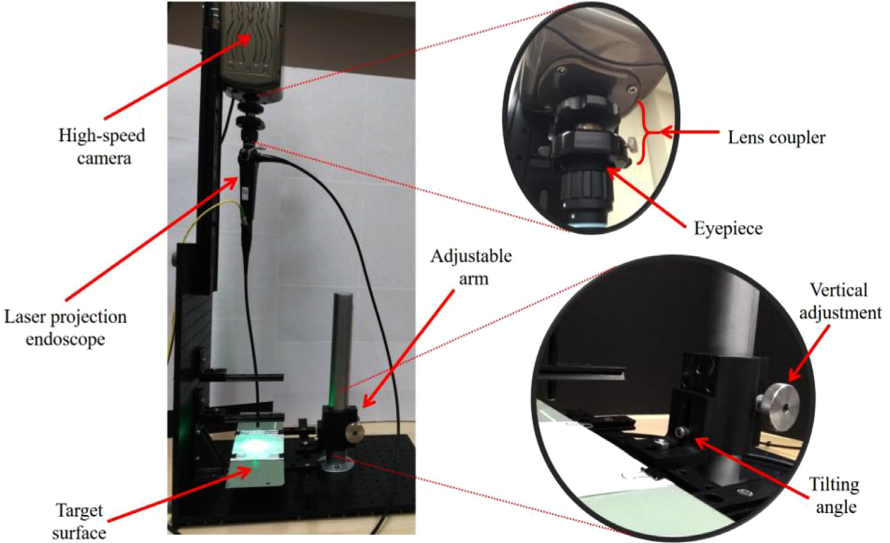
The employed setup for benchtop recordings.

Considering that images were taken from static surfaces, high frame rates were not required and the moderately low speed of 200 frames per second was used for data collection. The main benefit of reducing the frame rate is the increase in the integration time that we could get. Therefore, the target surface does not need to be very bright and instead of a xenon light, a conventional study incandescent lamp could be used for illuminating the target surface. The main problem with the xenon light was that it produced spatially nonuniform illumination (ie, the intensity of the light at different spatial locations was very different). This nonuniformity led to images with high-intensity divergence, which would unnecessarily complicate the required image processing algorithms. Therefore, a study lamp was employed as the light source for data collection.

Datasets

This study used recordings from a target surface at multiple working distances and multiple tilting angles for answering the research questions. The working distance was varied from 5 mm to 20 mm in 5-mm increments. The working distance was measured using a digital height gauge with an accuracy of 0.001’’ (approximately 0.03mm). The tilting angle was varied from − 15° to 15° in 5-degree increments. The following procedure was followed for measuring and adjusting the tilting angle. First, the target surface was leveled using a leveler. Then the distance between the front edge of the target surface (Figure 4) and the desk was measured using the digital height gauge. The same measurement was carried out for the back edge of the target surface. Let D and l denote the difference between the back and front measurements and the length of the target surface, respectively. Additionally, for a desired tilting angle let h_b and h_f denote heights of the front and back edges of the target surface from the table. Figure 4 depicts definitions of these quantities. Now, the trigonometric functions could be employed for measuring the tilting angle of the target surface (γ). Equation 4 shows the formula. Based on Equation 4, a negative angle corresponds to the case where the front edge of the target surface is higher than the back edge.

FIGURE 4.

A schematic for measuring the tilting angle.

$$\gamma =arcsin\left(\frac{h_b-h_f-D}{l}\right)$$ (4)

Finally, it is hard to adjust the setup for achieving the exact target working distances and tilting angles; therefore, the actual values deviated from the target values. Table 1 reflects the actual value of these parameters for each set of recording. However, in the reset of this paper groups will be referenced using their target values.

TABLE 1.

Actual Values of Working Distance and Tilting Angle for Each Target Group

	Working Distance Group
	5	10	15	20
Tilting angle group
−15	5.12, −15.6	9.93, −15.6	15.05, −15.6	20.06, −15.6
−10	5.06, −10.1	10.04, −10.1	15.27, −10.1	20.02, −10.1
−5	5.12, −5.1	10.07, −5.1	15.18, −5.1	20.05, −5.1
0	4.95, 0	10, 0	15.08, 0	20.12, 0
5	5.14, 5	10.05, 5	15.29, 5	20.05, 5
10	5.08, 10.3	10.08, 10.3	15.30, 10.3	20.15, 10.3
15	5.26, 15.6	10, 15.6	15.07, 15.6	20.07, 15.6

The First Number Represent the Actual Working Distance in mm, and the Second Number the Actual Tilting Angle in Degree.

Considering the aims of this research, square grid papers were attached to the target surface and they were recorded with the spatial resolution of 288 × 280 pixels, the frame rate of 200, and exposure time of 4900 μs. Subjective investigations showed that 1 mm grids were quite blurry and hard to detect at the working distance of 20 mm. Therefore, two different square grids with 1 mm and 2 mm spacings were used for data collection. Working distances of 5 mm, 10 mm, and 15 mm were recorded using 1mm-spacing grids and working distances of 15 mm and 20 mm were recorded using 2mm-spacing grids. The overlap between the two cases was used to investigate any possible effect of different grid sizes on the measurements. This is discussed in more detail in the Experiments and Results section.

Automatic detection of grid lines

The main aim of this study was to investigate the effect of nonlinear distortions in flexible endoscopy on horizontal measurements from the acquired images. Accurate detection of the grid lines from benchtop recordings was the prerequisite of that. Visual investigation of the recordings showed that grid lines in the images did not constitute straight lines but had some curvature. This characteristic is a classic case of the barrel distortion. Figure 5A shows an example image taken from the 1 mm grid at the working distance of 10 mm. Therefore, an automatic algorithm based on statistical image processing was developed to account for possible curvature of the grid lines. Frames of each video recording were averaged over the time and then a spatial averaging filter with the size of 2 pixels was applied. The following algorithm was then used for the detection of the vertical lines (ie, lines parallel to the y-axis). The filtered image was segmented in horizontal strips (ie, strips parallel to the x-axis) with the width of 10 pixels and maximum overlaps (ie, 9 pixels). The strip was averaged over the columns, and then locations of its local minimum were detected. A zero-vector mask was created, and locations of the minima were set to 1. This procedure was repeated for all horizontal strips, and all masks were concatenated vertically to create a binary image. The binary image at this stage underwent two morphological operations of dilation and erosion³⁰ using rectangular structuring elements with the size of 8 × 2 and 3 × 1 pixels. Finally, second-order polynomials were fitted on the regions with large areas. Figure 5 shows the outputs of the algorithm at different stages. The procedure for the detection of the horizontal lines (ie, lines parallel to the x-axis) followed similar steps. However, the filtered image was segmented in vertical strips (ie, strips parallel to the y-axis) instead. Also, the strips were averaged on the rows, zero-vector masks were concatenated horizontally, and rectangular structuring elements had the size of 2 × 8 and 1 × 3 pixels.

FIGURE 5.

Automatic detection of the grid lines. (A) Recording from 1 mm grids at the working distance of 10 mm. (B) The binary image showing locations of the minima. (C) Fitted second-order polynomials on the locations of the minima.

Pixel size

This study relies on a variable called the pixel size. This quantity could play a similar role to a scale on a printed map. Basically, we can multiply the uncalibrated pixel length of an object with this quantity and estimate its calibrated mm length. This number can be estimated as the ratio of the mm length of a target object to its pixel length during the horizontal calibration process. In this study, the target surfaces were calibrated square grids; hence, the mm lengths of sides of all blocks were known. Therefore, we could measure pixel lengths of sides of blocks from the image and then compute their corresponding values of pixel size. To that end, pixel lengths of sides of blocks were determined from the fitted curves (Figure 5C). Specifically, coordinates of intersections of all curves were determined with the precision of 0.1 pixel. Then, the pixel length of a side was computed as the Euclidian distance between its corresponding intersection points.

EXPERIMENTS AND RESULTS

Three experiments were conducted to answer the research questions of this study. This section presents details of each experiment, followed by results and related discussions.

Experiment 1

We saw in the Datasets section that two different grids with 1 mm and 2 mm spacings were used for collecting data from different working distances. Before proceeding with further analysis, we need to make sure that measurements from 1 mm and 2 mm grids are comparable. The following hypothesis was formed to test this.

H1: Pixel sizes computed from 1mm grids are significantly different from 2mm grids.

Rejection of H1 would indicate that measurements from 1 mm and 2 mm grids are comparable. The dataset for this experiment were images from 1 mm and 2 mm grids recorded at the working distance of 15 mm. Considering the possible effect of spatial location on the pixel size, two different groups of blocks were distinguished. The center group included all sides of blocks that were nearest to the center of the image-FOV. The periphery group included the farthest side of the blocks that were farthest from the center of the image-FOV. Figure 6 depicts the two groupings with their corresponding selected sides.

FIGURE 6.

Groupings for experiments 1 and 2. (A) The solid red blocks and the patterned blue blocks denote the center and the periphery groups. (B) The selected sides of an example image. Center of the image-FOV is denoted by a green cross mark.

The dependent variable for this experiment was the computed pixel size. The independent variables were grid sizes (1 mm vs 2mm) and groupings (center vs periphery). A two-way ANOVA was used to test H1. Since it is known that ANOVA is generally not robust to the violation of homogeneity of variance if groups have different sample sizes³¹, Levene’s test was first employed to check the homogeneity of variance. The test rejected the null hypothesis (P<.00001). Therefore, the analysis was carried out using M-estimators for the location with 1000 bootstrap, which provides ANOVA with robust performance for nonhomogeneous variance between groups.³² Table 2 reflects the results of this analysis.

TABLE 2.

Results of 2 × 2 Robust ANOVA

Variable	P
Grouping (G)	<0.00001
Grid size (S)	0.12
G × S	0.13

Based on Table 2, we see a nonsignificant effect of grid size on the pixel size. Therefore, we could conclude that measurements from 1 mm and 2 mm grids are comparable. Additionally, we see a significant effect for the grouping variable. It means that pixel sizes were significantly different between the center and the periphery groups. To better investigate this, experiment 2 was conducted.

Experiment 2

The aims of this experiment were to establish the dependence of the pixel size on its spatial location and then to quantify that dependence. Specifically, the effects of different groups (center vs. periphery as depicted in Figure 6) and different working distances on the pixel size were analyzed. Table 3 presents descriptive statistics of pixel size in different conditions.

TABLE 3.

Descriptive Statistics of Pixel Sizes

Working distance (mm)	Center		Periphery
	Mean (mm)	Std (mm)	Mean (mm)	Std (mm)
5	0.028	0.001	0.037	0.004
10	0.054	0.001	0.074	0.008
15	0.08	0.001	0.107	0.012
20	0.106	0.001	0.141	0.017

Figure 7 depicts how the pixel size changes between different groups and working distances.

FIGURE 7.

Variation in pixel size for different working distances and groups.

Based on Figure 7 we can hypothesize that,

H2: Pixel size is significantly smaller in the center group than the periphery group.

To test this hypothesis a new dataset was compiled. The dataset consisted of images from 1 mm grids recorded at the working distances of 5 mm and 10 mm and from 2 mm grids recorded at the working distances of 15 mm and 20 mm. The dependent variable for this experiment was the pixel size. The independent variables were groups (center vs periphery) and working distance. A two-way ANOVA could be used to test H2. It is known that ANOVA is not robust to the violation of homogeneity of variance if groups have different sample sizes³¹; therefore, Levene’s test was used to check the homogeneity of variance. Levene’s rejected the null hypothesis (P<.00001) indicating nonhomogeneity of variance between different groups. Consequently, the robust two-way ANOVA using M-estimators for the location with 1000 bootstrap samples was used instead.³² Table 4 reflects the results of the analysis.

TABLE 4.

Results of 2 × 4 Robust ANOVA

Variable	P
Groups (G)	<0.00001
Working distance (WD)	<0.00001
G × WD	<0.00001

Based on Table 4 we see a significant main effect of groups (center vs periphery), a significant main effect of the working distance, and a significant interaction effect. In order to pinpoint differences, robust post hoc analysis with 1000 bootstrap samples was used.³² The analysis showed significant differences between all contrasts. Figure 8 presents the boxplots of the pixel size for different groups and working distances.

FIGURE 8.

Boxplots of the pixel size for different groups and working distances.

Based on Figure 8 we could conclude that, at a fixed working distance, pixels from the center group have smaller pixel sizes than pixels from the periphery group. Additionally, the pixel size increases with the working distance, which was to be expected. Finally, as the working distance increases the disparity in the pixel size between the center and the periphery groups increases. This observation which concurs with the significant interaction effect presented in Table 4 has practical implications. Specifically, measurement errors due to the usage of pixel length for comparing sizes of two objects, one in the center and one in the periphery, increases with the working distance.

To quantify the effect of the spatial location of a pixel on its pixel size a different analysis was carried out. The pixel size of line segments highlighted in Figure 9A were computed. Also, the Euclidian distances between the center of all line segments and the center of the image-FOV were computed. Finally, a negative sign was assigned to the distance of blocks that were below the center of the image-FOV. Figure 9B presents a scatter plot of the pixel size for different distances from the center of the image-FOV. Second-order polynomials were fitted to measurements.

FIGURE 9.

(A) Selected line segments are shown in green dashed line, and the center of the image-FOV is denoted with a red cross mark. (B) Dependence of a pixel size on its distance from the center of the image-FOV and the working distance. The negative distance means blocks that were below the center of the image-FOV.

Based on Figure 9 the following conclusions can be made. First, the relationship between the pixel size and the distance from the center of the image-FOV is nonlinear. Second, curves are symmetrical around the center (ie, zero distance). This characteristic has practical implications. Basically, it means that pixel length cannot be used for within (and between) subject size comparison, unless the target objects have similar distances from the center of the image-FOV, in addition to similar working distances and zero tilting angle. For example, pixel length could not be used for comparing spatial features of a point on the left vocal fold to a similar point on the right vocal fold, unless those points have similar distances from the center of the image-FOV. Third, pixels in the center of the image have the smallest pixel size and as we move toward the periphery the value of pixel size increases. This characteristic has important practical implications. Moving the target tissue to the center of the image-FOV provides better spatial resolution and details in the captured images. Fourth, the curvature of plots increases with the working distance. That is the difference between pixel size in the center and the periphery increases with the working distance. This result concurs with results and discussion of Figure 8, and the significant interaction effect of Table 4.

The fitted second-order polynomials could be used to quantify the magnitude of variations in the pixel size between the center and the periphery. Table 5 shows the estimated values of pixel size at the center and periphery of the image-FOV. Considering the dependence of the pixel size on its spatial location, a possible simplistic approach for computing the mm length of an object could be to compute the average values of all pixel sizes in the image-FOV and use it as the pixel size. The mean column in Table 5 reflects this value. However, if this mean value is used for measuring the mm length of an object in the center and the periphery, some error will be introduced into the measurement. The percent value of this error for a center pixel was defined as the difference between the mean pixel size and the pixel size in the center divided by the mean value. A similar approach was followed for computing the percent difference of a periphery pixel. These values are presented in the last two columns of Table 5.

TABLE 5.

Estimated Values of Pixel Size

Working Distance (mm)	Center (mm)	Periphery (mm)	Mean (mm)	Center Diff. %	Periphery Diff. %
5	0.028	0.035	0.03	8	−16
10	0.053	0.067	0.058	8.1	−16.4
15	0.079	0.099	0.086	7.9	−14.6
20	0.106	0.131	0.115	7.8	−14.6

Combining previous results with Table 5 the following conclusions can be made. Despite the fact that the absolute value of difference increases with the working distance (more curvature in Figure 9B at larger working distances), yet the percentage of error remains relatively constant. This characteristic means that the nonlinear distortion mostly depends on the optical characteristics of the endoscope and it is relatively independent of the working distance. This independence translates into a simpler method for compensating the effect of such nonlinear distortions in horizontal measurements. This topic currently is being investigated and is the subject of a follow-up study. It is expected for the subsequent measurements to have significant implications to basic voice science and to future enhancement of clinical voice evaluation.

To put the results of Table 5 into perspective an extreme case of a within-subject size comparison scenario is presented. Let us consider the actual size of a lesion is reduced from 2 mm to 1.5 mm post an intervention. If the pre-intervention lesion is recorded at the working distance of 10 mm and on the periphery of the image, it would be presented by approximately 30 pixels. However, if the postintervention lesion is recorded at the same working but on the center of the image, it would be presented by approximately 28 pixels. That is, despite a 25% reduction in the mm length of the lesion we would get only a 6.7% reduction in the pixel length. This reduced sensitivity requires a bigger sample size in scientific research in order to achieve a significant effect.

Experiment 3

Experiments 1 and 2 were done at zero tilting angle (ie, imaging axis was perpendicular to the target surface). However, changes in the tilting angle could also lead to nonlinear distortions. The aim of this experiment was to study and quantify the effects of this parameter on horizontal measurements. Therefore, values of pixel size in three different groups at multiple working distances and multiple tilting angles were studies. Figure 10 shows the groupings that were used in this experiment. Recording at the working distance of 5 mm resulted in 14 line segments in the front and back groups and 18 line segments in the middle group. For all other working distances, all three groups had 22 line segments.

FIGURE 10.

Groupings for experiment 3. Solid red lines denote the back group, dotted green lines denote the middle group, and dashed blue lines denote the front group. (A) Groupings at the working distance of 5 mm (B) Groupings at the working distance of 15 mm.

We saw in experiment2 that the pixel size increases with the working distance. Considering that tilting the target surface decreases the working distance of one side of the image and increases the working distance of the other side, the following hypothesis was formed.

H3: pixel size is significantly different between back, middle, and front groups when the target surface gets tilted.

To test this hypothesis a new dataset was compiled. The dataset consisted of images from 1 mm grids recorded at working distances of 5 mm and 10 mm and from 2 mm grids recorded at working distances of 15 mm and 20 mm. The dependent variable for this experiment was the pixel size. The independent variables were groups (back, middle, and front), the working distance, and the tilting angle. Figure 11 presents the mean and standard deviation of the pixel size for the three groups at different working distances and tilting angles. A three-way ANOVA was used to test H3. Levene’s test rejected the null hypothesis (P <0.00001). Therefore, the analysis was carried out using trimmed means (0.2 trimming level), which provides ANOVA with robust performance for nonhomogeneous variance between groups.³² Table 6 reflects the results of the analysis. Based on this table we see all main effects were significant. Additionally, except for the Angle × WD, all other interaction effects were significant.

FIGURE 11.

Values of mean and standard deviation of pixel size. (A) Working distance of 5 mm, (B) Working distance of 10 mm, (C) Working distance of 15 mm, (D) Working distance of 20 mm.

TABLE 6.

Results of 7 × 4 × 3 ANOVA for Trimmed Means

Variable	P
Angle	0.0001
Working Distance (WD)	0.001
Groups (G)	0.0001
Angle × WD	0.86
Angle × G	0.001
G × WD	0.001
Angle × G × WD	0.001

Based on Figure 11 the following conclusions can be made. First, when the tilting angle is zero, the back and front groups have similar pixel sizes. However, as the magnitude of the tilting angle increases the difference in the pixel size of the back and front group increases. Specifically, at positive angles (ie, when the backside is higher) pixels in the back group have smaller pixel sizes than the front group (hence higher spatial resolution in the backside). Conversely, at negative angles, pixels in the front group have smaller pixel sizes than the back group. Second, crudely speaking, the behavior of the front group at a negative angle is similar to the behavior of the back group at a similar but positive angle, and vice versa. This characteristic indicates the presence of a specific symmetry in the distortion. Third, the standard deviations of different groups show dissimilar trends. The middle group exhibits the least variations and its behavior remains relatively constant for different tilting angles. However, as the tilting angle goes from −15° to 15° standard deviation of the pixel size in the front group (back) increases (decreases). This behavior may indicate a nonlinear dependence of the pixel size on the tilting angle and the spatial location of a target pixel. To quantify this behavior a further analysis was carried out.

The pixel sizes for line segments highlighted in Figure 12A were computed. Then, the Euclidian distance between the center of all line segments and the center of the image-FOV was computed. Then, a second-order polynomial curve was fitted for datapoints computed from each tilting angle. Figure 12B represents the result of this analysis for the working distance of 15 mm. It is noteworthy that, the negative sign denotes blocks that were below the center of the image-FOV.

FIGURE 12.

(A) The selected line segments are shown in green dashed line, and the center of the image-FOV is denoted with a red cross mark. (B) Dependence of a pixel size on its distance from the center of the image-FOV and the tilting angle at the working distance of 15 mm.

Based on Figure 12B we see significant differences between different curves. Specifically, when the tilting angle is zero, the minimum of the curve is near point zero (ie, the minimum pixel size is at the center of the image-FOV). However, when the tilting angle becomes positive the minimum of the curve (ie, position with the minimum pixel size and hence the highest spatial resolution) deviates from the center of the image-FOV and goes toward the negative direction (ie, toward the back of the target surface). Additionally, the magnitude of this deviation is positively correlated with the magnitude of the tilting angle. Conversely, when the tilting angle becomes negative the minimum of the curve deviates from the center of the image-FOV and goes toward the positive direction (moving toward the front of the target surface). Additionally, the magnitude of this deviation is positively correlated with the magnitude of the tilting angle. To quantify these qualitative observations, further analysis was carried out. The minimum of each curve was estimated using the analytical approach (ie, equating the derivative to zero). Figure 13 shows the distance of the minimum pixel size from the center of the image-FOV.

FIGURE 13.

Dependence of location with the highest spatial resolution on the tilting angle.

Another significant observation from Figure 12 is that at zero tilting angle the curve is symmetrical around the minimum point (which coincides with the center of the image-FOV). This means the points with similar distances from the center of the image-FOV would have similar pixel sizes. However, as the tilting angle starts to deviate, the curves become exceedingly asymmetric. That is, the dissimilarity between the two portions of the curves (left of the minimum and right of the minimum) increases with the magnitude of the tilting angle. To quantify these qualitative observations, further analysis was carried out. Let λ_min and λ_front denote the minimum pixel size and the pixel size at the front periphery of the image-FOV. Then, the percentage of difference at the front periphery (D_f) was defined as follows.

$$D_f=\frac{{\lambda }_{front}-{\lambda }_{min}}{{\lambda }_{min}}\times 100\%$$ (5)

The percentage of difference at the back periphery (D_b) was defined similarly. These values were computed for each working distance and tilting angle. Table 7 shows the results, which support the preceding qualitative discussions. Specifically, at negative tilting angles, pixel sizes are significantly larger at the back periphery (larger values of percentage of difference) and at positive tilting angles, pixel sizes are significantly larger at the front periphery (hence smaller spatial resolution). Additionally, as the magnitude of the tilting angle increases the percentage of difference from one side (the side that is getting away from the camera) increases while the other side (the side that is getting near to the camera) decreases. For example, at the working distance of 10 mm and the tilting angle of 15°, the pixel sizes at the front and back peripheries are 61.2% and 12.4% larger than the minimum pixel size. In summary, pixel sizes at the side of FOV that gets closer to the camera become more similar, whereas, the other side become more divergent.

TABLE 7.

The Percentage of Difference at the Back and Front Peripheries from Different Working Distances and Tilting Angles

Tilting angle	5mm		10mm		15mm		20mm
	Db%	Df%	Db%	Df%	Db%	Df%	Db%	Df %
−15°	61.5	17.9	59	13.8	55.5	11.5	59.6	14.3
−10°	46.1	16.5	45.3	15.2	43.5	14.6	42.2	14.3
−5°	28.7	18.1	29.4	18.6	35	19.1	34.1	18.8
0°	25.7	25.8	25.7	26.3	26.5	24.2	25.8	24.1
5°	18.1	31.4	19.5	33.7	19.8	31.3	20.5	32.8
10°	16.8	50.9	14.5	43.9	15.2	42.1	15.1	43.6
15°	12	65.7	12.4	61.2	13	59.9	12.7	60.3

The main goal of this article was to investigate the effect of two nonlinear distortions on horizontal measurements. To that end, we simulated a situation where an object with the actual length of 2 mm was placed at different locations of the FOV (front periphery, center, back periphery, and the location with the highest spatial resolution). Then we used the estimated value of pixel size (Figure 12B) for computing the pixel length of that object at the working distance of 10 mm and different tilting angles. Table 8 presents the results. The location with the highest spatial resolution (denoted as maximum in Table 8) was determined analytically (ie, equating the derivative to zero) from curves in Figure 12B.

TABLE 8.

Estimated Uncalibrated Length (ie, Pixel Length) of a 2 mm Object at Different Locations of the FOV and Different Tilting Angles

Tilting angle	Front	Center	Back	Maximum
−15°	36	39	25	40
−10°	34	39	27	40
−5°	32	38	29	38
0°	30	38	30	38
5°	29	38	32	38
10°	25	36	32	37
15°	26	40	37	41

Table 8 clearly demonstrates the effect of spatial location and tilting angle on the uncalibrated size (ie, pixel length) of an object in flexible endoscopy. For example, for a constant spatial location in the back periphery the uncalibrated size of the object could increase by 48% if the tilting angle changes from −15° to 15°. Also, for a constant tilting angle of 15° the uncalibrated size of the object could increase by 57.7% if the object moves from the minimum resolution location to the maximum resolution location in the FOV. Finally, we can see the interaction effect of grouping (front, center, back) and the tilting angle. Specifically, at zero tilting angle the uncalibrated size of an object on the front periphery increases by 26.7% if that object moves to the center of the image-FOV. However, at the tilting angle of 15°, the increase could be as high as 53.8%.

DISCUSSIONS

Imaging techniques are widely employed in clinical practice. The fields of speech-language pathology and laryngology are not an exception. However, the access for direct functional observation of the laryngeal tissues is not trivial, and therefore, the visualization is channeled through an endoscopic instrument. Hence, the functionality and characteristics of the endoscope determine the characteristics of the acquired images. For example, rigid endoscopy is based on transoral insertion, which limits the types of stimuli that can be elicited. Also, the unnatural retraction of the tongue³³ required for adequate laryngeal exposure may alter the voice production system and hence may not reflect the natural function of the phonatory system. For example, research has shown that the presence of a rigid endoscope could significantly change the fundamental frequency and quality of the produced voice,³⁴ which may support a modified function of the phonatory mechanism during the rigid endoscopy. Flexible endoscopy helps address some of these concerns. Also, flexible endoscopes provide the possibility of simultaneous aerodynamic measurements.^35–37 This could provide significant information about the complex interactions between kinematics, aerodynamics, and the produced acoustic of the phonatory mechanism. Additionally, coupling a laser calibrated flexible endoscope¹⁰ to an HSV system and recording synchronized aerodynamic measurements could help us tease apart the effect of individual differences on the phonatory mechanism. Last but not least, flexible scopes have been associated with higher success rates in adult³⁸ and pediatric^39,40 populations. However, flexible endoscopes are associated with nonlinear distortions. The main aim of this paper was to quantify the effects of two different sources of nonlinear distortions in the images acquired from a fiberoptic flexible endoscope. The first source stems from the wide-angle lens that is used in the flexible endoscope in order to compensate for short working distances and hence maximizing the FOV. The second source of nonlinearity stems from changes in the imaging angle. A significant error can be introduced into measurements if these distortions are not compensated for. Two different interpretations of the effects of these distortions are presented here. The first interpretation relates to the usage of uncalibrated measurements (ie, pixel lengths) and quantifies the magnitude of error in comparing pixel length of objects from different locations of the image-FOV. Whereas, the second interpretation relates to calibrated measurements (ie, estimating the mm lengths) in the absence of proper compensation methods. This interpretation quantifies the magnitude of error in estimating the mm length of objects from different locations of the image-FOV. Experiments 1 and 2 demonstrated the significant effect of spatial location of a pixel on its mm size. Based on results of Table 5 pixels in the periphery could have about 26.4% lower spatial resolution than pixel in the center. This means that if pixel lengths are used for comparing two similar objects one in the center and one the periphery, length of the object in the center will be over-estimated by 26.4%. Considering the mm measurement, a simplistic solution could be to compute the average pixel size and then use it for conversion from pixel into mm. Based on results of Table 5 this approach could lead up to 8.1% overestimation of the object in the center and up to 14% underestimation of the object in the periphery. Experiment 3 investigated the effect of tilting angle and showed its significant effect on measurements. Specifically, Table 8 showed that pixel length of an object in the periphery of the image-FOV could changes by 48% if the tilting angle goes from − 15° to 15°. If the average pixel size (Table 5, column Mean) is used and the effect of tilting angle is not compensated for, calibrated mm measurements could have significant error. Specifically, at the tilting angle of 15° the mm length on one side of the periphery could be underestimated by 34%.

The focus of this study was on nonlinear distortion from a laser-calibrated laryngeal fiberoptic flexible endoscope and their effect of horizontal measurement. However, the results may provide insights and motivation for further analysis of other types of endoscopes, as well as, other endoscopic procedures (eg, gastroendoscopy, colonoscopy). Specifically, the first nonlinear distortion was due to the wide-angle lens of the fiberoptic flexible endoscopes. Considering that distal-chip flexible endoscopes, gastroendoscopy, and colonoscopy also use wide-angle lenses, one may expect to see some residual distortions. However, the exact magnitude of distortion would be different from this study and should be investigated in a separate study. Rigid endoscopes have a narrower angle of view and hence the small-angle approximation may be valid. Therefore, the effect of the first source on nonlinear distortion could be minimal in rigid endoscopes. On the other hand, the effect of the imaging angle seems to be universal. Therefore, it is expected for accuracy of measurements from rigid endoscopy, distal-chip flexible endoscopes, gastroendoscopy, and colonoscopy to depend on the imaging angle. However, the exact magnitude of that distortion could be different from fiberoptic endoscopes and should be investigated in a separate study. To address this need, we are planning to use a similar approach and evaluate the distortions of distal-chip videoendoscopy systems, which would quantify the effect of tilting angle and spatial location on validity and reliability of horizontal measurements. Considering the popularity and widespread usage of distal chip videoendoscopy systems in clinical settings, such study is warranted to provide more immediate clinical value.

Implications and findings from this study seem to extend beyond horizontal measurements. For example, in Figure 5C we see that parallel lines exhibit a bowing effect in the captured images. This may indicate that subjective visual assessments of laryngeal images captured from fiberoptic flexible endoscopes for assessment of vocal fold bowing may get biased. Figure 12A shows that when the imaging angle is not perpendicular, parallel lines may result in divergent lines in the image. This may indicate that vocal folds that are in fact parallel may be captured as divergent ones in laryngeal images (regardless of the imaging modality) if the imaging angle is not perpendicular. Last but not least, the objective and subjective measurements of asymmetry have been used in previous literature.^19,41 However, the investigated nonlinear distortions could significantly change the accuracy of those subjective assessments and objective measurements.

CONCLUSION

This study was motivated by performing calibrated (ie, mm) horizontal measurement from a laser-calibrated HSV system. The system was designed based on a fiberoptic flexible endoscope. Two different sources of nonlinear distortions in the fiberoptic flexible endoscope were investigated, the wide-angle lens used in flexible endoscopes, and the deviation in the imaging angle. It was shown that the first source of distortion, the wide-angle lens, results in a pixel size (ie, the conversion scale from pixel into mm) that depends on the spatial location of that pixel. More precisely, it was shown that if the imaging axis is perpendicular, all pixels with similar distances to the center of the image-FOV will have similar pixel sizes. Additionally, it was shown that as we move away from the center of the image-FOV the pixel size increases. A different interpretation of this observation would be that the spatial resolution of the image decreases as we move away from the center of the image-FOV toward its periphery. Therefore, keeping the region of interest in the center of the image-FOV would improve the details of the captured image. Studying the second source of nonlinear distortion, the effect of imaging angle, showed that it disturbs the radial symmetry of the images. That is, spatial resolution of points with similar distance to the center of the image-FOV become dissimilar, and also that dissimilarity increases with an increase in the tilting angle. Additionally, this distortion leads to the dislocation of the points with the highest spatial resolutions from the center of the image- FOV. The analysis showed that the combined nonlinear distortions could result in calibrated horizontal measurement errors up to 65.7%.

REFERENCES

- 1.Roy N, Barkmeier-Kraemer J, Eadie T, et al. Evidence-based clinical voice assessment: a systematic review. Am J Speech-Language Pathol. 2013;22:212–226. [DOI] [PubMed] [Google Scholar]
- 2.Kendall KA, Leonard RJ, eds. Laryngeal Evaluation: Indirect Laryngoscopy to High-Speed Digital Imaging. Thieme; 2011. [Google Scholar]
- 3.Dejonckere PH, Bradley P, Clemente P, et al. A basic protocol for functional assessment of voice pathology, especially for investigating the efficacy of (phonosurgical) treatments and evaluating new assessment techniques. Eur Arch Oto-rhino-laryngology. 2001;258:77–82. [DOI] [PubMed] [Google Scholar]
- 4.Naunheim MR, Carroll TL. Benign vocal fold lesions: Update on nomenclature, cause, diagnosis, and treatment. Curr Opin Otolaryngol Head Neck Surg. 2017;25:453–458. 10.1097/MOO.0000000000000408. [DOI] [PubMed] [Google Scholar]
- 5.Patel RR, Eadie T, Paul D, et al. Recommended protocols for instrumental assessment of voice: American speech-language-hearing association expert panel to develop a protocol for instrumental assessment of vocal function. Am J Speech-Language Pathol. 2018;27:887–905. 10.1044/2018_ajslp-17-0009. [DOI] [PubMed] [Google Scholar]
- 6.Deliyski DD, Petrushev PP, Bonilha HS, et al. Clinical implementation of laryngeal high-speed videoendoscopy: Challenges and evolution. Folia Phoniatr Logop. 2008;60:33–44. [DOI] [PubMed] [Google Scholar]
- 7.Mehta DD, Hillman RE. Current role of stroboscopy in laryngeal imaging. Curr Opin Otolaryngol Head Neck Surg. 2012;20:429. [DOI] [PMC free article] [PubMed] [Google Scholar]
- 8.Powell ME, Deliyski DD, Zeitels SM, et al. Efficacy of videostroboscopy and high-speed videoendoscopy to obtain functional outcomes from perioperative ratings in patients with vocal fold mass lesions. J Voice. 2019. 10.1016/j.jvoice.2019.03.012. (in Press). [DOI] [PMC free article] [PubMed]
- 9.Ghasemzadeh H, Deliyski D, Ford D, et al. Method for vertical calibration of laser-projection transnasal fiberoptic high-speed videoendoscopy. J Voice. 2019. (in Press)[Epub ahead of print]. [DOI] [PMC free article] [PubMed]
- 10.Deliyski DD, Shishkov M, Mehta DD, et al. Laser-calibrated system for transnasal fiberoptic laryngeal high-speed videoendoscopy. J Voice. 2019. (in Press[Epub ahead of print]). [DOI] [PMC free article] [PubMed]
- 11.Speyer R, Wieneke GH, Kersing W, et al. Accuracy of measurements on digital videostroboscopic images of the vocal folds. Ann Otol Rhinol Laryngol. 2005;114:443–450. [DOI] [PubMed] [Google Scholar]
- 12.Rosen CA. Stroboscopy as a research instrument: development of a perceptual evaluation tool. Laryngoscope. 2005;115:423–428. [DOI] [PubMed] [Google Scholar]
- 13.Dailey SH, Kobler JB, Hillman RE, et al. Endoscopic measurement of vocal fold movement during adduction and abduction. Laryngoscope. 2005;115:178–183. [DOI] [PubMed] [Google Scholar]
- 14.Patel R, Donohue KD, Unnikrishnan H, et al. Kinematic measurements of the vocal-fold displacement waveform in typical children and adult populations: quantification of high-speed endoscopic videos. J Speech, Lang Hear Res. 2015;58:227–240. [DOI] [PMC free article] [PubMed] [Google Scholar]
- 15.Iwahashi T, Ogawa M, Hosokawa K, et al. A detailed motion analysis of the angular velocity between the vocal folds during throat clearing using high-speed digital imaging. J Voice. 2016;30:770.e1–770.e8. [DOI] [PubMed] [Google Scholar]
- 16.Powell ME, Deliyski DD, Hillman RE, et al. Comparison of videostroboscopy to stroboscopy derived from high-speed videoendoscopy for evaluating patients with vocal fold mass lesions. 2016;25(Andrade 2009):2011–2013. doi: 10.1044/2016. [DOI] [PMC free article] [PubMed] [Google Scholar]
- 17.Noordzij JP, Woo P. Glottal area waveform analysis of bsenign vocal fold lesions before and after surgery. Ann Otol Rhinol Laryngol. 2000;109:441–446. 10.1177/000348940010900501. [DOI] [PubMed] [Google Scholar]
- 18.Patel RR, Dubrovskiy D, Döllinger M. Measurement of glottal cycle characteristics between children and adults: physiological variations. J Voice. 2014;28:476–486. [DOI] [PMC free article] [PubMed] [Google Scholar]
- 19.Bonilha HS, Deliyski DD, Gerlach TT. Phase asymmetries in normophonic speakers: visual judgments and objective findings. Am J Speech-Language Pathol. 2008;17:367–376. [DOI] [PMC free article] [PubMed] [Google Scholar]
- 20.Švec JG, Šram F, Schutte HK. Videokymography in Voice Disorders: What to Look For? Ann Otol Rhinol Laryngol. 2007;116:172–180. [DOI] [PubMed] [Google Scholar]
- 21.Schade G, Leuwer R, Kraas M, et al. Laryngeal morphometry with a new laser “clip on” device. Lasers Surg Med. 2004;34:363–367. [DOI] [PubMed] [Google Scholar]
- 22.Herzon GD, Zealear DL. New laser ruler instrument for making measurements through an endoscope. Otolaryngol Neck Surg. 1997;116: 689–692. [DOI] [PubMed] [Google Scholar]
- 23.Patel RR, Donohue KD, Lau D, et al. In vivo measurement of pediatric vocal fold motion using structured light laser projection. J Voice. 2013;27:463–472. [DOI] [PMC free article] [PubMed] [Google Scholar]
- 24.Luegmair G, Mehta DD, Kobler JB, et al. Three-Dimensional Optical Reconstruction of Vocal Fold Kinematics Using High-Speed Video With a Laser Projection System. IEEE Trans Med Imaging. 2015;34: 2572–2582. [DOI] [PMC free article] [PubMed] [Google Scholar]
- 25.Hibi SR, Bless DM, Hirano M, et al. Distortions of videofiberoscopy imaging: reconsideration and correction. J Voice. 1988;2:168–175. [Google Scholar]
- 26.Deng JJ, Hadwin PJ, Peterson SD. The effect of high-speed videoendoscopy configuration on reduced-order model parameter estimates by Bayesian inference. J Acoust Soc Am. 2019;146:1492–1502. [DOI] [PMC free article] [PubMed] [Google Scholar]
- 27.Alzamendi GA, Manriquez R, Hadwin PJ, et al. Bayesian estimation of vocal function measures using laryngeal high-speed videoendoscopy and glottal airflow estimates: An in vivo case study. J Acoust Soc Am. 2020;147:EL434–EL439. [DOI] [PMC free article] [PubMed] [Google Scholar]
- 28.Smith WJ, Smith WJ. Modern Optical Engineering. 3rd, ed. New York: Mcgraw-hill; 2000. [Google Scholar]
- 29.Fannin TE, Grosvenor T. Clinical Optics. Butterworth-Heinemann; 2013. [Google Scholar]
- 30.Dougherty ER, Lotufo RA. Hands-on Morphological Image Processing. 59. SPIE press; 2003. [Google Scholar]
- 31.Field A, Miles J, Field Z. Discovering Statistics Using R. Sage publications; 2012. [Google Scholar]
- 32.Wilcox RR. Introduction to Robust Estimation and Hypothesis Testing. Academic press; 2011. [Google Scholar]
- 33.Chandran S, Hanna J, Lurie D, et al. Differences between flexible and rigid endoscopy in assessing the posterior glottic chink. J Voice. 2011;25:591–595. [DOI] [PubMed] [Google Scholar]
- 34.Ng ML, Bailey RL. Acoustic changes related to laryngeal examination with a rigid telescope. Folia Phoniatr Logop. 2006;58:353–362. [DOI] [PubMed] [Google Scholar]
- 35.Kobler JB, Zeitels SM, Hillman RE, et al. Assessment of vocal function using simultaneous aerodynamic and calibrated videostroboscopic measures. Ann Otol Rhinol Laryngol. 1998;107:477–485. [DOI] [PubMed] [Google Scholar]
- 36.Mehta DD, Deliyski DD, Zeitels SM, et al. Integration of transnasal fiberoptic high-speed videoendoscopy with time-synchronized recordings of vocal function. in Technology, Vol. 1 of Normal and Abnormal Vocal Folds Kinematics: High Speed Digital Phonoscopy (HSDP), Optical Coherence Tomography (OCT) & Narrow Band Imaging (NBI®), 1st ed. (CreateSpace, Scotts Valley, CA, 2015). ePhonoscope. 2015:105–114.
- 37.Zañartu M, Mehta DD, Ho JC, et al. Observation and analysis of in vivo vocal fold tissue instabilities produced by nonlinear source-filter coupling: a case study. J Acoust Soc Am. 2011;129:326–339. [DOI] [PMC free article] [PubMed] [Google Scholar]
- 38.Milstein CF, Charbel S, Hicks DM, et al. Prevalence of laryngeal irritation signs associated with reflux in asymptomatic volunteers: impact of endoscopic technique (rigid vs. flexible laryngoscope). Laryngoscope. 2005;115:2256–2261. [DOI] [PubMed] [Google Scholar]
- 39.Gray SD, Smith ME, Schneider H. Voice disorders in children. Pediatr Clin North Am. 1996;43:1357–1384. [DOI] [PubMed] [Google Scholar]
- 40.Chait DH, Lotz WK. Successful pediatric examinations using nasoendoscopy. Laryngoscope. 1991;101:1016–1018. [DOI] [PubMed] [Google Scholar]
- 41.Mehta DD, Deliyski DD, Quatieri TF, et al. Automated measurement of vocal fold vibratory asymmetry from high-speed videoendoscopy recordings. J Speech, Lang Hear Res. 2011;54:47–54. [DOI] [PMC free article] [PubMed] [Google Scholar]