

Abstract
“Resting‐state” functional magnetic resonance imaging (rs‐fMRI) is widely used to study brain connectivity. So far, researchers have been restricted to measures of functional connectivity that are computationally efficient but undirected, or to effective connectivity estimates that are directed but limited to small networks. Here, we show that a method recently developed for task‐fMRI—regression dynamic causal modeling (rDCM)—extends to rs‐fMRI and offers both directional estimates and scalability to whole‐brain networks. First, simulations demonstrate that rDCM faithfully recovers parameter values over a wide range of signal‐to‐noise ratios and repetition times. Second, we test construct validity of rDCM in relation to an established model of effective connectivity, spectral DCM. Using rs‐fMRI data from nearly 200 healthy participants, rDCM produces biologically plausible results consistent with estimates by spectral DCM. Importantly, rDCM is computationally highly efficient, reconstructing whole‐brain networks (>200 areas) within minutes on standard hardware. This opens promising new avenues for connectomics.
Keywords: connectomics, effective connectivity, generative model, hierarchy, regression dynamic causal modeling, resting state
“Resting‐state” functional magnetic resonance imaging (rs‐fMRI) is widely used to study brain connectivity. So far, researchers have been restricted to measures of functional connectivity that are computationally efficient but undirected, or to effective connectivity estimates that are directed but limited to small networks. Here, we show that a method recently developed for task‐fMRI—regression dynamic causal modeling (rDCM)—extends to rs‐fMRI and offers both directional estimates and scalability to whole‐brain networks.
1. INTRODUCTION
“Resting‐state” functional magnetic resonance imaging (rs‐fMRI) has long been used to examine the functional organization of the brain during unconstrained cognition when no specific experimental manipulations are present (Biswal, Van Kylen, & Hyde, 1997; Biswal, Yetkin, Haughton, & Hyde, 1995). Specifically, resting‐state fMRI has revealed spontaneous (endogenous) fluctuations in the blood oxygen level dependent (BOLD) signal that are highly structured across the brain (Fox et al., 2005; Greicius, Supekar, Menon, & Dougherty, 2009; Raichle et al., 2001). Over the last two decades, rs‐fMRI has become one of the most vibrant fields in neuroimaging (for reviews, see Smith et al., 2013; van den Heuvel & Hulshoff Pol, 2010) and now plays a central role in disciplines such as connectomics (Craddock et al., 2013) and network neuroscience (Bassett & Sporns, 2017). This is partly due to its practical simplicity, which renders rs‐fMRI amenable to subject populations that may otherwise struggle to adhere to complex cognitive tasks, such as neuropsychiatric patients, elderly people, or infants.
So far, rs‐fMRI data has been analyzed predominantly in terms of functional connectivity, which represents statistical interdependencies among BOLD signal time series from spatially distinct regions of the brain (Friston, 2011). The simplest way to assess functional connectivity is by computing Pearson's correlation coefficient between the respective BOLD signal time series. Other measures of functional connectivity include partial correlation, coherence, mutual information, and independent component analysis (for a comprehensive review, see Karahanoglu & Van De Ville, 2017).
Regardless of the exact approach, these statistical techniques have revealed a number of large‐scale networks of correlated temporal patterns in the resting brain. These resting‐state networks (RSNs) are characterized by fairly coherent time courses across its set of inherent components, whereas time courses are sufficiently distinct between networks (Beckmann, DeLuca, Devlin, & Smith, 2005; Fox & Raichle, 2007; Smith et al., 2009). The most prominent RSN is arguably the default mode network (DMN) which is also frequently referred to as the task‐negative network (Raichle et al., 2001; Shulman et al., 1997). The DMN was initially discovered as a consistent set of brain regions that showed deactivations across various attention‐demanding, goal‐oriented, nonself‐referential tasks (for a comprehensive review, see Raichle, 2015). By now, it is clear that the DMN can also be active in specific goal‐oriented paradigms such as autobiographical tasks (Spreng, 2012), thinking about others and oneself, or remembering the past and planning the future (Buckner, Andrews‐Hanna, & Schacter, 2008). Since the discovery of the DMN, similar patterns of resting‐state coherence have been identified in most cortical systems, giving rise to other RSNs such as the dorsal attention network (DAN; Corbetta & Shulman, 2002; Fox, Corbetta, Snyder, Vincent, & Raichle, 2006), salience network (SAN; Dosenbach et al., 2007; Menon & Uddin, 2010), and central executive network (CEN; Spreng, Sepulcre, Turner, Stevens, & Schacter, 2013; Spreng, Stevens, Chamberlain, Gilmore, & Schacter, 2010). All RSNs persist even during sleep and under various forms of anaesthesia (Picchioni, Duyn, & Horovitz, 2013; but see Tagliazucchi & Laufs, 2014), and show high heritability (Fornito et al., 2011; Glahn et al., 2010), suggesting that they might represent fundamental organizing principles of the human brain.
Importantly, mapping the macroscopic functional connectome from rs‐fMRI data has not only shed light on the organizational principles in the healthy human brain, but also in disease. Aberrant resting‐state functional connectivity has been observed in most psychiatric and neurological disorders (Baker et al., 2019; Buckholtz & Meyer‐Lindenberg, 2012; Bullmore & Sporns, 2009; Fornito, Zalesky, & Breakspear, 2015; Stam, 2014). For example, psychiatric diseases including schizophrenia (Baker et al., 2014; Friston, Brown, Siemerkus, & Stephan, 2016; Lui et al., 2015), depression (Greicius et al., 2007; Wang, Hermens, Hickie, & Lagopoulos, 2012), and autism (Courchesne et al., 2007; Hahamy, Behrmann, & Malach, 2015) have all been associated with pathological alterations in resting‐state functional connectivity.
Despite these profound contributions to our understanding of the organizing principles of the human brain, measures of functional connectivity essentially describe statistical properties of the data and do not reveal how the data were caused or generated. As such, functional connectivity does not directly capture mechanisms at a latent level of neuronal interactions. Furthermore, measures of functional connectivity are undirected and thus do not capture asymmetries in reciprocal connections. This is problematic because asymmetries in the coupling among brain regions have been repeatedly found both in terms of anatomy (Felleman & Van Essen, 1991; Markov et al., 2014) and function (Frässle et al., 2016; Gazzaniga, 2000; Stephan, Marshall, Penny, Friston, & Fink, 2007; Zeki & Shipp, 1988).
In contrast, effective connectivity refers to directed interactions among brain regions and can be assessed by exploiting a generative model of the latent (hidden) neuronal states and how these give rise to the observed measurements (Friston, 2011). One of the most widely used generative modeling frameworks for inferring effective connectivity from fMRI data is dynamic causal modeling (DCM; Friston, Harrison, & Penny, 2003), and variants of DCM have been established to model the resting state, including stochastic DCM (Daunizeau, Friston, & Kiebel, 2009; Li et al., 2011) and spectral DCM (Friston, Kahan, Biswal, & Razi, 2014). While capable of more mechanistic accounts of functional integration during the resting state, these models are restricted to relatively small networks due to computational limitations.
We recently introduced a novel variant of DCM for fMRI—termed regression dynamic causal modeling (rDCM; Frässle, Lomakina, et al., 2018; Frässle et al., 2017)—that differs from previous DCMs in several aspects. Most important, rDCM is computationally highly efficient and scales gracefully to very large networks including hundreds of nodes, paving the way for whole‐brain effective connectivity analyses (Frässle et al., 2021). Furthermore, the model can exploit structural connectivity information to constrain inference on directed functional interactions or, where no such information is available, infer optimally sparse representations of whole‐brain connectivity patterns. While rDCM was initially designed to work with experimentally controlled perturbations (i.e., task data), the current implementation can, in principle, also by applied to rs‐fMRI data. However, this has not been tested thoroughly so far. Here, we assess the face validity and construct validity of rDCM for inferring effective connectivity during the resting state. To this end, we conducted comprehensive simulation analyses and compared rDCM against spectral DCM as an alternative and well‐established generative model of rs‐fMRI data for small networks. This comparison made use of a large empirical resting‐state fMRI dataset acquired by the Bipolar‐Schizophrenia Network on Intermediate Phenotypes (B‐SNIP) consortium (Tamminga et al., 2013). Finally, we showed that rDCM gracefully scales to large networks with more than 200 areas and enables fast inference on whole‐brain effective connectivity patterns from rs‐fMRI data at the time‐scale of minutes.
2. METHODS AND MATERIALS
2.1. Regression DCM
2.1.1. General overview
Regression DCM (rDCM) is a novel variant of DCM for fMRI that enables effective connectivity analyses in large (whole‐brain) networks (Frässle, Lomakina, et al., 2018; Frässle et al., 2017). This can be achieved by applying several modifications and simplifications to the original DCM framework. In brief, these include (i) translating state and observation equations from time to frequency domain using the Fourier transformation (under stationarity assumptions), (ii) replacing the nonlinear biophysical model of hemodynamics with a linear hemodynamic response function (HRF), (iii) applying a mean field approximation across regions (i.e., connectivity parameters targeting different regions are assumed to be independent), and (iv) specifying conjugate priors on neuronal (i.e., connectivity and driving input) parameters and noise precision. These modifications essentially reformulate the linear DCM in the time domain as a Bayesian linear regression in the frequency domain, resulting in the following likelihood function:
| (1) |
Here, Yr is the dependent variable in region r that is explained as a linear mixture of afferent connections from other regions and direct (driving) inputs. Specifically, Yr is the Fourier transformation of the temporal derivative of the measured signal in region r. Furthermore, yr represents the measured BOLD signal in region r, X is the design matrix (comprising a set of regressors and explanatory variables), uk is the k th experimental input, and the hat symbol denotes the discrete Fourier transform (DFT). Additionally, θr represents the parameter vector comprising all connections ar,1, …, ar,R and all driving input parameters cr,1, …, cr,K targeting region r. Finally, τr denotes the noise precision parameter for region r and IN × N is the identity matrix (where N denotes the number of data points). Choosing appropriate priors on the parameters and hyperparameters in Equation (1) (see Frässle et al., 2017) results in a generative model that can be used for inference on the directed connection strengths and inputs.
Under this formulation, inference can be done very efficiently by (iteratively) executing a set of analytical Variational Bayes (VB) update equations concerning the sufficient statistics of the posterior density. In addition, one can derive an expression for the negative (variational) free energy (Friston, Mattout, Trujillo‐Barreto, Ashburner, & Penny, 2007). The negative free energy represents a lower‐bound approximation to the log model evidence that accounts for both model accuracy and complexity. Hence, the negative free energy offers a sensible metric for scoring model goodness and thus serves as a criterion for comparing competing hypotheses (Bishop, 2006). We have recently further augmented rDCM by introducing sparsity constraints into the likelihood of the model in order to allow automatic pruning of fully connected network structures (Frässle, Lomakina, et al., 2018). Notably, the present article focuses on the original implementation of rDCM without sparsity constraints. A comprehensive description of the generative model of rDCM, including the mathematical details of the neuronal state equation underlying the likelihood function in Equation (1), can be found elsewhere (Frässle, Lomakina, et al., 2018; Frässle et al., 2017).
2.1.2. Application to resting‐state data
While rDCM was originally designed to work with experimentally controlled perturbations (i.e., task data), it is also possible to fit the model to rs‐fMRI data. This can be achieved by “switching off” driving inputs (i.e., setting all input parameters ci,j to zero in the absence of experimental inputs uk) and, in order to explain activity in any given region, relying on measured data (in the Fourier domain) in regions from which afferent connections are received; compare the likelihood function in Equation (1). This means that, in contrast to stochastic variants of DCM, the generative model does not explicitly represent endogenous fluctuations in neuronal activity and has no concept of stochastic “innovations” or similar ways noise can drive neuronal activity intrinsically. Instead, endogenous fluctuations of BOLD signal in any given region are explained as a linear mixture of intrinsic fluctuations from other regions. Hence, while the model can still account for regional endogenous fluctuations of the BOLD signal during the resting state, the current formulation of rDCM blurs the strict separation between (latent) state and (measured) observation levels that is otherwise a characteristic feature of DCMs. This formulation renders rDCM conceptually similar to a multivariate autoregressive model in the frequency domain (compare the discussion in Frässle et al., 2017).
It is worth emphasizing that we do not wish to portray the current formulation of rDCM as a theoretically optimal treatment of “resting state” fMRI data; instead, it should be seen as offering a pragmatic solution for enabling whole‐brain directed connectivity estimates from rs‐fMRI data. Specifically, while the derivation of rDCM (see Frässle et al., 2017 for details) enhances algebraic tractability and computational speed, the ensuing loss of separation between state and observation levels represents a conceptual limitation, for example, with regard to separating state and observation noise (see Section 4). In previous work, we have shown that, despite its inherent simplifications, rDCM works well in application to task data (Frässle, Lomakina, et al., 2018; Frässle et al., 2017, 2021). In this study, we examine the face validity and construct validity of rDCM in its specific application to rs‐fMRI data. Concerning face validity, we investigate whether the particular formulation of rDCM allows for veridical inference on effective connectivity, using simulated BOLD data fluctuations that were generated by means of a deterministic generative model with stochastic driving inputs and regional hemodynamic variability (see below). With regard to construct validity, we apply rDCM to empirical fMRI data and compare the results to those obtained by spectral DCM (Friston, Kahan, Biswal, & Razi, 2014), an alternative and established model of effective connectivity for rs‐fMRI data.
2.2. Synthetic data
First, we evaluated the face validity of rDCM in simulation studies by generating synthetic rs‐fMRI data for which the ground truth (i.e., the data‐generating parameter values) were known. In particular, we assessed model parameter recovery in four different linear DCMs and evaluated performance as a function of the repetition time (TR) and signal‐to‐noise ratio (SNR) of the synthetic data. Each of the models comprised four regions, yet differed with regard to the degree of sparsity of the network architecture (Figure 1a). More precisely, Model 1 represented a full network where all regions were connected via reciprocal connections, Model 2 comprised 75% of all possible connections, Model 3 comprised 50% of all possible connections, and Model 4 was the sparsest network with only 25% of all connections present. Please note that this simulation work was restricted to a small network with only four regions in order to allow comparability of rDCM with spectral DCM (Friston, Kahan, Biswal, & Razi, 2014), which represents an alternative variant of DCM for rs‐fMRI data (see below).
FIGURE 1.
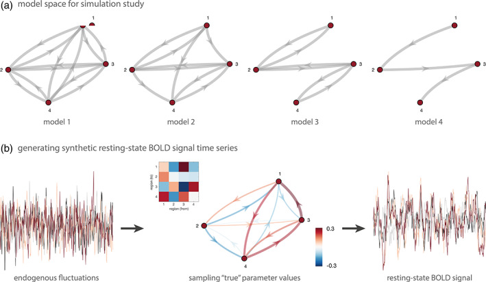
Pipeline for simulation studies on regression DCM (rDCM). (a) Model space for the simulation studies dedicated to assessing the face validity of rDCM for resting‐state data. Four different network structures were utilized that varied in their degree of sparsity. Model 1 represents a fully connected model where all regions are coupled via reciprocal connections (i.e., 12 connectivity parameters), Model 2 represents a network with 75% of all connections present (i.e., 9 connectivity parameters), Model 3 represents a network with 50% of all connections present (i.e., 6 connectivity parameters), and Model 4 represents the sparsest network with only 25% of all connectivity present (i.e., 3 connectivity parameters). (b) Regional endogenous fluctuations were generated from an AR(1) process and then utilized as driving inputs in the respective model. Specifically, we here used a classical deterministic DCM to generate synthetic data. Model parameters were sampled from their prior distributions and then utilized to generated synthetic BOLD signal time series that resembled the characteristic amplitudes and slow fluctuations observed during the resting state. Measurement noise, generated from another AR(1) process, was added on top of the predicted BOLD signal time series
For each model, synthetic fMRI data were then generated to resemble the characteristic amplitude and low‐frequency fluctuations seen in resting‐state BOLD signal time series. To this end, we followed an established procedure described in previous work (Friston, Kahan, Biswal, & Razi, 2014; Razi, Kahan, Rees, & Friston, 2015) and implemented in the MATLAB function DEM_demo_induced_fMRI.m as part of SPM12 (version R7487, Wellcome Centre for Human Neuroimaging, London, UK, http://www.fil.ion.ucl.ac.uk). In brief, endogenous neuronal fluctuations were generated independently for each region by using an AR(1) process with an autoregression coefficient of 1/2. The endogenous neuronal fluctuations were scaled to a standard deviation of 1/4. These values were previously identified by Friston, Kahan, Biswal, and Razi (2014) as producing realistic BOLD signal changes. Region‐wise endogenous fluctuations were then utilized as driving inputs to a classical deterministic DCM (Friston et al., 2003). Similarly, measurement noise was generated independently for each region from another AR(1) process and added on top of the simulated BOLD signal time courses. Hence, synthetic resting‐state fMRI data were thus generated using a generative model that was different from both rDCM and spectral DCM. This established procedure ensured a fair basis for the comparison between rDCM and spectral DCM by avoiding any obvious biases towards one or the other DCM variant. Synthetic resting‐state fMRI data were simulated to mimic an experiment of 10 minutes duration. Importantly, BOLD signal time series were generated under a variety of different signal‐to‐noise ratios (SNR = [0.5 1 3]) and repetition times (TR = [2 s, 1 s, 0.5 s]) in order to evaluate the performance of rDCM as a function of data quality and sampling rate, respectively. Here, SNR was defined as the ratio between the standard deviation of the signal and the standard deviation of the AR(1)‐type measurement noise (i.e., SNR = σsignal/σnoise).
For each of the four models and each combination of SNR and TR, 20 different sets of observations (“synthetic subjects”) were generated. To this end, the generating (“true”) parameter values of each simulation were sampled from the prior distributions of the endogenous parameters. Values of connectivity parameters too close to zero (i.e., |ai,j| < 0.05) were discarded and re‐sampled in order to ensure sufficient information transfer between regions. Notably, the sampling procedure also included hemodynamic parameters. In other words, in our simulations, the synthetic BOLD signal time series displayed variability in the hemodynamic response across both regions and subjects. This allowed us to test whether rDCM can faithfully recover “true” connectivity parameters in the context of biologically realistic hemodynamic variability, despite the method's simplistic assumption of a fixed HRF (Frässle et al., 2017).
Examples of endogenous fluctuations and ensuing synthetic BOLD signal time series are shown in Figure 1b. Note that, as a result of the low‐pass filtering of the hemodynamic response function, the BOLD signal is much smoother than the underlying endogenous fluctuations. The resulting BOLD signal time series are biologically realistic and show the characteristic slow (low‐frequency) fluctuations typically observed during the resting state.
Based on the synthetic data, model inversion was performed by making use of the function tapas_rdcm_estimate.m from the rDCM toolbox as implemented in the Translational Algorithms for Psychiatry Advancing Science (TAPAS) toolbox (www.translationalneuromodeling.org/tapas). Model parameter recovery was then assessed by computing (i) the root‐mean‐squared‐error (RMSE) and (ii) the Pearson's correlation coefficient (r) between the inferred and the generating (“true”) parameter values in order to quantify how much the estimated posterior parameter values differed from the ground truth.
2.3. Empirical data
Second, we examined the construct validity of rDCM in relation to spectral DCM. For this, we applied both models to an empirical rs‐fMRI dataset and compared the results. Specifically, we made use of a large dataset collected by the Bipolar‐Schizophrenia Network on Intermediate Phenotypes (B‐SNIP‐1) consortium, with one measure being rs‐fMRI (Tamminga et al., 2013, 2014). Overall, participants with psychosis (including schizophrenia, schizoaffective disorder, and psychotic bipolar I disorder), their first‐degree relatives, and demographically matched healthy participants were collected for the B‐SNIP‐1 dataset.
2.3.1. Participants
The data utilized in the present study were acquired by the B‐SNIP‐1 consortium as part of a large cross‐sectional study of intermediate phenotypes in psychosis (Tamminga et al., 2013). The B‐SNIP‐1 consortium included five sites in the United States: (i) Baltimore, (ii) Chicago, (iii) Dallas, (iv) Detroit and Boston, and (v) Hartford. The sites used identical study protocols, and considerable effort was taken to harmonize recoding and testing conditions across sites by utilizing identical stimulus presentation and recording equipment. Furthermore, experimenters across sites were cross‐trained and frequently monitored to ensure comparable data collection procedures. A detailed study description is provided elsewhere (Tamminga et al., 2013, 2014).
The current methodological study is a precursor to a broader project that evaluates the clinical utility of whole‐brain directed connectivity estimates in the context of the psychosis spectrum, using the BSNIP‐1 data. However, applying rDCM to these clinical questions requires an initial assessment of its face and construct validity in the context of resting‐state fMRI data. A natural choice of dataset for assessment of construct validity was the healthy control sample of the B‐SNIP‐1 dataset, as it was acquired under the same conditions as the patient dataset. Healthy participants were recruited from the local communities. They were without lifetime psychotic disorders and had no first‐degree relatives with a history of psychotic or bipolar disorder according to the Family History Research Diagnostic Criteria (Andreasen, Endicott, Spitzer, & Winokur, 1977). Overall, 459 healthy participants were assessed by the B‐SNIP‐1 consortium. For the current study, only those participants were included that had: (i) a complete data set comprising all relevant demographical information and neuroimaging data and (ii) sufficiently high data quality of the fMRI measurements (exclusion criteria related to data quality are listed below). This yielded a final sample of 196 healthy participants that were included in our study (80 females, 116 males; age: 38.3 ± 12.5 years; age range: 15–64 years). The study protocol was approved by the institutional review board at each local site. All participants provided written informed consent prior to inclusion and after they obtained a complete description of the study.
2.3.2. Experimental procedure
While in the MR scanner, participants were asked to fixate on a small cross presented on the screen, and to remain alert with eyes open and head still. These instructions were designed to help prevent participants from falling asleep, provide an experimental control over visual inputs and eye movements, and reduce head movements. Head movements were further restricted by having participants' heads placed in a custom‐build head‐coil cushion.
2.3.3. Data acquisition
Structural and functional MRI data were acquired at the five sites of the B‐SNIP‐1 consortium. These included the University of Maryland School of Medicine (Baltimore), Commonwealth Research Center at Harvard Medical School (Boston), University of Illinois Medical Center (Chicago), University of Texas Southwestern Medical Center (Dallas), and Olin Neuropsychiatry Research Center at the Institute of Living (Hartford). Participants were scanned on 3 Tesla MR scanners of different manufacturers, including GE Signa, Siemens Trio, Philips Achieva, and Siemens Allegra. For comprehensive details on data acquisition parameters across the different sites, see Supporting Information S1.
2.3.4. Data preprocessing
Preprocessing of the MR data was performed using fMRIPrep (version 1.4.1; Esteban et al., 2019) which is based on Nipype (version 1.2.0; Gorgolewski et al., 2011) and was specifically designed for automated high‐quality preprocessing in the context of large‐scale datasets. We here utilized the standard preprocessing pipeline from fMRIPrep, which comprised the following steps.
The T1‐weighted (T1w) anatomical image was corrected for intensity nonuniformity (INU) with N4BiasFieldCorrection (Tustison et al., 2010), distributed with ANTs 2.2.0 (Avants, Epstein, Grossman, & Gee, 2008), and used as T1w reference throughout the workflow. The T1w reference was then skull‐stripped with a Nipype implementation of the antsBrainExtraction workflow. Brain tissue segmentation of cerebrospinal fluid (CSF), white matter (WM), and gray matter (GM) was performed on the brain‐extracted T1w image using fast (Zhang, Brady, & Smith, 2001), distributed with FSL 5.0.9 (Jenkinson, Beckmann, Behrens, Woolrich, & Smith, 2012). Volume‐based spatial normalization to the MNI standard space was performed through nonlinear registration with antsRegistration (ANTs 2.2.0), using brain‐extracted versions of both T1w reference and T1w template (MNI152NLin2009cAsym; Fonov, Evans, McKinstry, Almli, & Collins, 2009).
Functional images were preprocessed by first generating a reference volume (BOLD reference) and its skull‐stripped version by making use of a custom methodology of fMRIPrep. Head‐motion parameters with respect to the BOLD reference (transformation matrices, and six corresponding rotation and translation parameters) were estimated before any spatiotemporal filtering using mcflirt (Jenkinson, Bannister, Brady, & Smith, 2002). Slice‐timing correction was performed to account for differences in acquisition timing across slices. A deformation field to correct for susceptibility distortions was estimated based on the fieldmap‐less approach in fMRIPrep (Wang et al., 2017). This procedure utilizes the T1w reference from the same subject as the undistorted target in a nonlinear registration scheme. To maximize the similarity between T2* contrast of the EPI scan and the T1w reference, the intensities of the latter are inverted. To regularize the optimization of the deformation field, displacements are constrained to be nonzero only along the phase‐encoding direction and the magnitude of displacements is modulated with an average fieldmap template (Treiber et al., 2016). Based on the estimated susceptibility distortion, unwarped BOLD images were calculated for a more accurate co‐registration with the anatomical reference by resampling functional images onto their original, native space through a single, composite transform to correct for head‐motion and susceptibility distortions. This was followed by co‐registration to the T1w reference using flirt (Jenkinson & Smith, 2001) with the boundary‐based registration cost function (Greve & Fischl, 2009), implemented in FSL 5.0.9 (Jenkinson et al., 2012). Co‐registration was configured with nine degrees of freedom to account for remaining distortions in the BOLD images. The corrected and coregistered functional images were then normalized into MNI standard space (MNI152NLin2009cAsym; Fonov et al., 2009) by making use of the warps obtained from the spatial normalization of the T1w reference (see above).
2.3.5. Estimation of confound regressors
From the functional images, fMRIPrep computes several time series of potentially confounding influences that can be used subsequently (during the extraction of BOLD signal time series) as confound regressors to correct for variance of no interest. Here, we will focus only on those confound regressors that were utilized in the present analysis; for a comprehensive list of all confound regressors estimated by fMRIPrep, see elsewhere (Esteban et al., 2019).
In brief, framewise displacement (FD) and DVARS (Power, Barnes, Snyder, Schlaggar, & Petersen, 2012) were calculated by making use of their implementations in Nipype, following the definitions by Power et al. (2014). Furthermore, three global signals were extracted within the CSF, WM, and a whole‐brain mask. Additionally, the head motion estimates (translation and rotation) obtained during preprocessing were utilized as confound regressors. The confound regressors derived from head motion estimates and global signals were expanded with the inclusion of temporal derivatives and quadratic terms for each (Friston, Williams, Howard, Frackowiak, & Turner, 1996; Satterthwaite et al., 2013). Furthermore, frames that exceeded a threshold of 0.5 mm for FD or 1.5 for standardized DVARS were annotated as motion outliers and marked using a stick regressor. Finally, regressors encoding a discrete cosine set with a 128 s cut‐off were utilized for high‐pass filtering.
2.3.6. Exclusion criteria
In addition to fMRIPrep, we utilized MRIQC (version 0.15.1; Esteban et al., 2017) for quality control of the neuroimaging data. Specifically, we ran MRIQC with the default parameters, with the exception of the FD threshold being adjusted to 0.5 mm. Participants were excluded from further effective connectivity analysis if any of the following image quality metrics derived by MRIQC were above/below the specified threshold. For the structural images, exclusion criteria were defined as: (i) “QI1” >0.005, (ii) “overlap_tpm_csf” <0.1, (iii) “overlap_tpm_gm” <0.3, and (iv) “overlap_tpm_wm” <0.45. In brief, “QI1” represents the proportion of artifact‐corrupted voxels as assessed using the algorithm described by Mortamet et al. (2009). Furthermore, “overlap_tpm_*” represents the overlap between the tissue probability maps (TPMs) estimated from the anatomical image and the corresponding maps from the MNI152NLin2009cAsym template. For the functional images, exclusion criteria were specified as: (i) “aqi” >0.025, and (ii) “fd_perc” >20.0. In brief, “aqi” is AFNI's mean quality index computed by the 3dTqual routine, and “fd_perc” represents the percentage of scans with a FD above the FD threshold with respect to the entire time series. A full description of the metrics is available from https://mriqc.readthedocs.io/en/latest/measures.html.
2.3.7. Time series extraction: small networks
To evaluate the construct validity of rDCM in application to resting‐state fMRI data, we examined functional integration during the resting state from two perspectives: modes and nodes in rs‐fMRI (Friston, Kahan, Razi, Stephan, & Sporns, 2014). First, we examined effective connectivity among key intrinsic networks of the human brain (i.e., modes). Specifically, we investigated the established anticorrelations between the task‐negative DMN, engaged during rest and internally directed tasks, and task‐positive networks, engaged during externally oriented tasks. These anticorrelations have been proposed to serve as a fundamental characteristic of endogenous or spontaneous fluctuations during the resting state (Fox et al., 2005; Raichle, 2015; Smith et al., 2009; but see section 4 and Fox, Zhang, Snyder, & Raichle, 2009).
To this end, we selected in a first step four modes of interest, comprising the DMN (Buckner et al., 2008; Raichle, 2015), DAN (Corbetta & Shulman, 2002; Fox et al., 2006), SAN (Dosenbach et al., 2007; Menon & Uddin, 2010), and CEN (Spreng et al., 2010; Spreng et al., 2013). Masks for each of the four RSNs were created by making use of previously published templates of those RSNs (Shirer, Ryali, Rykhlevskaia, Menon, & Greicius, 2012) and are displayed in Figure 2a.
FIGURE 2.
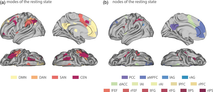
Masks for the empirical analysis of the B‐SNIP‐1 resting‐state data. (a) Masks comprising four key intrinsic networks (i.e., modes) of the resting state. Specifically, we included the default mode network (DMN; yellow), dorsal attention network (DAN; orange), salience network (SAN; red), and the central executive network (CEN; purple). (b) Masks comprising 15 subcomponents of three key intrinsic networks (DMN, DAN, and SAN) of the resting state. For the DMN (blueish colors): posterior cingulate cortex (PCC), anterior medial prefrontal cortex (aMPFC), and left and right angular gyrus (lAG and rAG). For the SAN (yellowish colors): dorsal anterior cingulate cortex (dACC), left and right anterior insula (lAI and rAI), and left and right anterior prefrontal cortex (lPFC and rPFC). For the DAN (reddish colors): left and right frontal eye fields (lFEF and rFEF), left and right inferior frontal gyrus (lIFG and rIFG), and left and right inferior parietal sulcus (lIPS and rIPS). All masks were taken from the templates published in Shirer et al. (2012)
In a second step, we investigated effective connectivity during the resting state not only at the level of entire networks, but at the level of the regional components (nodes) of those networks. To this end, we restricted ourselves to the DMN, DAN, and SAN, in line with previous work on the hierarchical organization of RSNs by Zhou et al. (2018). Consistent with Zhou et al. (2018), we subdivided the three key intrinsic networks as follows: For the (core) DMN, we identified four regions: posterior cingulate cortex (PCC), anterior medial prefrontal cortex (aMPFC), and left and right angular gyrus (lAG and rAG). For the DAN, we identified 6 regions: left and right frontal eye fields (lFEF and rFEF), left and right inferior frontal gyrus (lIFG and rIFG), and left and right inferior parietal sulcus (lIPS and rIPS). For the SAN, we identified five regions: dorsal anterior cingulate cortex (dACC), left and right anterior insula (lAI and rAI), and left and right anterior prefrontal cortex (lPFC and rPFC). This yielded a total of 15 regions of interest (ROIs) from which BOLD signal time series were extracted. Again, we utilized the templates provided by Shirer et al. (2012) as masks for the respective ROIs (Figure 2b). More specifically, we utilized the respective masks that had been obtained by Shirer et al. (2012) by sub‐dividing modes into their subcomponents.
Delineating the components of the intrinsic networks allowed for a more fine‐grained analysis of effective connectivity during the resting state and for disentangling functional integration within and between networks. It also served as a more challenging test scenario for rDCM given the increase in network size and, thus, number of free connectivity parameters. Having said this, the resulting network sizes are still an order of magnitude smaller than what is possible using rDCM. However, for the assessment of construct validity, we deliberately restricted ourselves to relatively small networks in order to allow for a comparison between rDCM and spectral DCM (but see below for an application of rDCM to rs‐fMRI data from a whole‐brain network with more than 200 regions).
For either of the two analysis pipelines (i.e., “modes” and “nodes”), BOLD signal time series were extracted as the first eigenvariate of all voxels within the respective mask. Time series were mean centered and confound‐related variance was removed (by regression using all nuisance regressors included in the first‐level GLM).
2.3.8. Time series extraction: whole‐brain network
Finally, to demonstrate that rDCM can infer effective connectivity patterns during the resting state at the whole‐brain level, we utilized the Human Brainnetome atlas as a whole‐brain parcellation scheme (Fan et al., 2016). The Brainnetome atlas represents a connectivity‐based parcellation derived from diffusion weighted imaging (DWI) data. In brief, the atlas comprises 246 distinct parcels (123 per hemisphere), including 210 cortical and 36 subcortical regions. Due to signal dropouts in the raw functional images (especially in inferior temporal regions near the skull base), BOLD signal time series could not be extracted for all regions defined by the Brainnetome atlas. Overall, 221 regions could be extracted in all participants. However, in order to ensure interhemispheric consistency of the network, we further reduced this set by excluded regions that were present in only one hemisphere.
This yielded a total of 212 brain regions from which sensible BOLD signal time series could be obtained in every participant. As for the small‐network analyses, BOLD signal time series were then extracted as the first eigenvariate of all voxels within the respective mask. Time series were mean centered and confound‐related variance was removed (by regression using all nuisance regressors included in the first‐level GLM).
2.3.9. rDCM analysis
The extracted BOLD signal time series from the previous step were then utilized for subsequent effective connectivity analyses using rDCM. For this, we constructed fully connected networks where all modes/regions were coupled to each other via reciprocal connections. This yielded a total of 16 free parameters for the 4‐mode network and 225 free parameters for the 15‐node network (all possible inter‐regional connections and inhibitory self‐connections), as well as 18,260 free parameters for the whole‐brain network (all inter‐regional connections present in the structural connectome of the Brainnetome atlas and inhibitory self‐connections) to be estimated. Again, model inversion was performed by utilizing the routine tapas_rdcm_estimate.m from the rDCM toolbox as implemented in TAPAS. For the small networks, parameter estimates obtained with rDCM were then compared to those obtained by spectral DCM (SPM12; version R7487), using the identical BOLD signal time series. To this end, two analyses were performed: First, we assessed the consistency of parameter estimates at the group level by computing the Pearson's correlation between the group‐averaged posterior parameter estimates of the two DCM variants. Second, we studied the consistency of parameter estimates at the individual level (rather than at the group level) by computing, for each connection separately, the Pearson's correlation across the individual posterior parameter estimates of the two DCM variants. Significance of associations was quantified by a threshold of p <.05. Note that, for the whole‐brain network, no comparison between rDCM and spectral DCM was possible.
3. RESULTS
3.1. Simulations
3.1.1. Face validity
First, we performed comprehensive simulation studies to assess the face validity of rDCM for modeling resting‐state fMRI data. To this end, we tested whether rDCM can recover generating (“true”) parameter values in four different four‐region networks (Figure 1) under various settings of SNR and TR of the synthetic data.
Overall, model parameter values could be recovered faithfully over a wide range of SNR and TR settings, for all four network architectures (Figure 3a, Table 1, and Figure S1). Specifically, root‐mean‐squared‐errors (RMSE) were below 0.15 in all tested cases. On average, we found the mean RMSE to range from 0.09 for model 1 to 0.04 for model 4 for the most challenging case of high measurement noise (SNR = 0.5) and low sampling rate (TR = 2 s). Note that, the absolute RMSE value is difficult to interpret as it will depend on the scaling of the data; hence, values should only be interpreted in a relative manner as they allow comparison across different data settings (i.e., SNR, TR) as well as across the different DCM variants. The average Pearson's correlation coefficient () ranged from .70 for Model 1 to .95 for Model 4 for the low‐SNR‐slow‐TR scenario, and thus showed a pattern highly consistent with the RMSE. Notably, averaging was performed by (i) transforming individual correlation coefficients to z‐space using Fisher r‐to‐z transformation, (ii) computing mean as well as lower and upper bound of the 95% confidence interval in z‐space, and finally (iii) back‐transforming estimates to r‐space. Overall, we observed an (expected) dependence of model parameter recovery on the sparsity of the network, with the most accurate results being observed for the simplest Model 4 with the lowest number of free parameters (Figure 3a). Furthermore, we observed a strong dependence of model parameter recovery performance on the data quality, suggesting that rDCM can infer upon connection strengths more faithfully for higher SNR settings of the (synthetic) BOLD signal time series. A similar effect was observed for the sampling rate (i.e., TR). Specifically, model parameter recovery performance of rDCM improved for faster TR settings, although this was somewhat less pronounced as the effect of the SNR (see Figure S1). The observed dependencies of model parameter recovery performance on SNR and TR settings are consistent with previous simulation analyses on rDCM in the context of task‐based data (Frässle, Lomakina, et al., 2018; Frässle et al., 2017).
FIGURE 3.
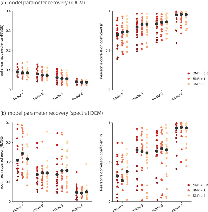
Model parameter recovery for regression DCM and spectral DCM. (a) Model parameter recovery for synthetic resting‐state fMRI data in terms of the root mean squared error (left) and the Pearson's correlation coefficient (right) between the inferred and the “true” data‐generating parameter values for regression DCM (rDCM), and (b) spectral DCM. Each colored dot represents the respective RMSE or Pearson's correlation coefficient for an individual synthetic subject. Black dots represent the mean RMSE or mean Pearson's correlation coefficient, averaged across all 20 synthetic subjects. Note that, averaging of the individual Pearson's correlation coefficients was performed in z‐space (see main text). Results are shown for four different network architectures, where model 1 is the most complex (full) model and model 4 is the sparsest network. Furthermore, results are shown for an exemplary repetition time (TR) of 2 s and three different signal‐to‐noise ratios (SNRs): 0.5 (red), 1 (orange), and 3 (yellow)
TABLE 1.
Model parameter recovery for regression DCM and spectral DCM
| SNR | RMSE | Pearson's correlation | |
|---|---|---|---|
| Mean [95% CI] | Mean [95% CI] | ||
| Regression DCM (rDCM) | |||
| Model 1 | 0.5 | 0.092 [0.084 0.099] | .70 [.63 .76] |
| 1 | 0.088 [0.080 0.096] | .73 [.66 .79] | |
| 3 | 0.088 [0.079 0.096] | .74 [.67 .79] | |
| Model 2 | 0.5 | 0.082 [0.071 0.092] | .80 [.73 .85] |
| 1 | 0.076 [0.066 0.085] | .83 [.77 .87] | |
| 3 | 0.074 [0.065 0.083] | .84 [.79 .88] | |
| Model 3 | 0.5 | 0.062 [0.053 0.072] | .84 [.79 .88] |
| 1 | 0.058 [0.049 0.068] | .86 [.81 .89] | |
| 3 | 0.057 [0.048 0.067] | .86 [.82 .90] | |
| Model 4 | 0.5 | 0.041 [0.037 0.045] | .95 [.92 .97] |
| 1 | 0.039 [0.036 0.042] | .96 [.93 .98] | |
| 3 | 0.039 [0.036 0.042] | .96 [.93 .98] | |
| Spectral DCM | |||
| Model 1 | 0.5 | 0.209 [0.174 0.245] | .32 [.21 .43] |
| 1 | 0.244 [0.203 0.285] | .27 [.11 .41] | |
| 3 | 0.217 [0.169 0.264] | .38 [.30 .46] | |
| Model 2 | 0.5 | 0.138 [0.111 0.165] | .66 [.52 .76] |
| 1 | 0.146 [0.118 0.174] | .64 [.50 .74] | |
| 3 | 0.145 [0.119 0.172] | .62 [.49 .72] | |
| Model 3 | 0.5 | 0.138 [0.103 0.172] | .64 [.50 .75] |
| 1 | 0.157 [0.119 0.194] | .67 [.54 .77] | |
| 3 | 0.158 [0.123 0.193] | .66 [.51 .77] | |
| Model 4 | 0.5 | 0.048 [0.033 0.062] | .93 [.88 .96] |
| 1 | 0.043 [0.035 0.052] | .94 [.90 .97] | |
| 3 | 0.051 [0.035 0.067] | .93 [.88 .96] | |
Note: Model parameter recovery for synthetic resting‐state fMRI data in terms of root mean squared error (left) and Pearson's correlation coefficient (right) between the inferred and “true” data‐generating parameter values for regression DCM (rDCM) and spectral DCM. Averaging of the individual Pearson's correlation coefficients as well as computing the 95% confidence interval (CI) was achieved by (i) transforming individual correlation coefficients to z‐space using Fisher r‐to‐z transformation, (ii) computing mean as well as lower and upper bound of the 95% CI in z‐space, and finally (iii) back‐transforming estimates to r‐space. Results are reported for four different network architectures, where model 1 is the most complex (full) model and model 4 is the sparsest network. Furthermore, results are reported for an exemplary repetition time (TR) of 2 s and three different signal‐to‐noise ratios (SNRs): 0.5, 1, and 3.
3.1.2. Comparison to spectral DCM
In a second step, we compared the model parameter recovery performance of rDCM with results obtained with spectral DCM (Friston, Kahan, Biswal, & Razi, 2014), which represents an alternative variant of DCM for fMRI that is suited to model resting‐state data. Importantly, spectral DCM has already been assessed in terms of face validity (Friston, Kahan, Biswal, & Razi, 2014), construct validity (Razi et al., 2015), and test–retest reliability (Almgren et al., 2018). Consequently, spectral DCM serves as a useful benchmark against which rDCM can be challenged.
Spectral DCMs were fitted to the exact same synthetic BOLD signal time series that have previously been utilized for rDCM. As before, model parameter recovery of spectral DCM improved as a function of network sparsity (Figure 3b and Table 1). However, the dependence of model parameter recovery on the characteristics of the synthetic fMRI data was less clear for spectral DCM: while no obvious dependence on data quality (i.e., SNR) could be observed, model parameter recovery showed a tendency to improve as a function of sampling rate (see Figure S2), which is consistent with previous work (Friston, Kahan, Biswal, & Razi, 2014). When comparing parameter recovery performance across the two DCM variants, overall, rDCM performed better than spectral DCM. More specifically, rDCM and spectral DCM were on par for the simplest Model 4, whereas for all other network architectures, rDCM outperformed spectral DCM in terms of RMSE and Pearson's correlation coefficient. This pattern was observed across all SNR and TR settings.
In summary, our simulation analyses provide evidence for the face validity of rDCM in application to synthetic resting‐state fMRI data in a relatively broad range of SNR and TR settings (Figures S1 and S2).
3.2. Empirical analyses: 4‐mode network
3.2.1. Effective connectivity during resting state
Next, we investigated the construct validity of rDCM in comparison to spectral DCM, using an empirical rs‐fMRI dataset. We here used the 196 healthy participants from the B‐SNIP‐1 consortium (Tamminga et al., 2013) described earlier (see Section 2).
First, we investigated effective connectivity among four key modes of the resting state (Figure 2a), namely the DMN, DAN, SAN, and CEN. Individual connectivity parameters were estimated in a fully connected network using rDCM. Model inversion resulted in biologically plausible connectivity patterns (Figure 4a). Specifically, we observed pronounced inhibitory afferent (inward) and efferent (outward) connections between the DMN, representing the task‐negative network, and the DAN and SAN, representing task‐positive networks. Additionally, we observed excitatory reciprocal connections between DAN and SAN. Interestingly, the CEN exerted a relatively strong excitatory influence on the DMN and simultaneously received a (weaker) positive influence from the DMN. Furthermore, the CEN was coupled positively to the DAN and negatively to the SAN.
FIGURE 4.

Effective connectivity among key modes of the resting state. (a) Group‐averaged posterior parameter estimates during the resting state as inferred with regression DCM (rDCM), and (b) spectral DCM (spDCM). Note that, in order to make the correlation between group‐averaged connectivity estimates of the two DCM variants more easily visible, color was scaled in relation to the maximal values of each method. Hence, we utilize slightly different color scales for the two DCM variants for illustration purposes. (c) Consistency of group‐level parameter averages between rDCM and spDCM. Shown are the group‐averaged inter‐regional connectivity estimates (top) as well as the Pearson's correlation coefficient (r) among them (bottom). Dots are colored using the rDCM color scale. (d) Consistency of individual parameter estimates for each connection separately; here, shown for the connection with the weakest (left) and strongest association (right) between the two DCM variants. Dots are colored using the rDCM color scale. (e) Range of correlation coefficients across all 12 connections of the 4‐mode network. Each colored dot represents the Pearson's correlation coefficient for an individual inter‐regional connection and the black dot denotes the mean Pearson's correlation coefficient, averaged across all connections. Note that, averaging of individual Pearson's correlation coefficients was performed in z‐space (see main text)
Based on the posterior parameter estimates, one can compute a metric of hierarchy strength as the difference between averaged absolute efferent and afferent connections for each of the four intrinsic networks of the resting state. This approach has been used by a previous DCM study on the hierarchical organization of RSNs (Zhou et al., 2018), and is similar to approaches used for analyzing hierarchical projections in the monkey brain (Goulas, Uylings, & Stiers, 2014) and the hierarchical organization of the prefrontal cortex in humans (Nee & D'Esposito, 2016). Importantly, this definition of “hierarchy” should not be confused with other accounts that relate to layer‐specificity of forward and backward connections (Felleman & Van Essen, 1991; Markov et al., 2014). Instead, the present definition simply refers to the degree of influence that one mode exerts over others (for a comprehensive review of alternative definitions of hierarchy, see Hilgetag & Goulas, 2020). The total hierarchy strength was indicative of a hierarchical organization of the four networks with the DMN at the bottom (−0.12), predominantly serving as a sink, and the other task‐positive networks ranking higher (DAN: 0.05, SAN: 0.02, CEN: 0.05), predominantly serving as neuronal drivers. This finding is consistent with previous observations on the hierarchical organization of RSNs (Sridharan, Levitin, & Menon, 2008; Zhou et al., 2018).
3.2.2. Comparison to spectral DCM
As for the simulations above, we again compared our findings from rDCM to those obtained by spectral DCM, using the identical BOLD signal time series. We observed that, at the group level, effective connectivity patterns were highly consistent across the two DCM variants (Figure 4b). In brief, spectral DCM also revealed pronounced inhibitory afferent and efferent connections between the DMN and the DAN and SAN, as well as excitatory reciprocal connections among DAN and SAN. The only (qualitative) difference between spectral DCM and rDCM results was observed in how the CEN integrated into this network. While, consistent with the rDCM results, efferent connections from the CEN to the DMN and DAN were excitatory, afferent connections to the CEN from DMN and DAN were inhibitory. With regard to the coupling between CEN and SAN, spectral DCM and rDCM again yielded consistent results. This similarity between the two DCM variants was also represented by a very high Pearson's correlation coefficient between the group‐level inter‐regional connectivity estimates (r = .85, p <.001; Figure 4c).
In a second step, we investigated the consistency of parameter estimates at the individual level (rather than at the group level) for each connection separately. At the individual level, connections showed some variability in the degree of consistency between the two DCM variants. While for some connections, the Pearson's correlation between rDCM and spectral DCM parameter estimates was relatively weak, as seen for the connection from CEN to DAN (r = .13, p = .06; Figure 4d, left), others showed much higher consistency, like the connection from DAN to CEN (r = .67, p <.001; Figure 4d, right). Overall, the mean Pearson's correlation coefficient, averaged across connections, was = .38 [.27 .48] (Figure 4e). Again, averaging was performed by (i) transforming individual correlation coefficients to z‐space using Fisher r‐to‐z transformation, (ii) computing mean as well as lower and upper bound of the 95% confidence interval in z‐space, and finally (iii) back‐transforming estimates to r‐space. Despite the observed variability, our results suggest that, across connections, there is significant evidence for consistency across parameter estimates from the two DCM variants at the individual level, as assessed using a one‐sample t‐test after Fisher r‐to‐z transformation of the correlation coefficients (t [1,11] = 6.40, p <.001).
3.3. Empirical analysis: 15‐node network
3.3.1. Effective connectivity during resting state
Next, we aimed to study effective connectivity during the resting state not only at the level of entire networks, but at the level of the regional components of those networks. To this end, we restricted our analysis to the DMN, DAN, and SAN and, consistent with Zhou et al. (2018), divided these three networks into 15 subcomponents (Figure 2b). This yielded four regions for the DMN (PCC, aMPFC, lAG, and rAG), five regions for the SAN (dACC, lAI, rAI, lPFC, and rPFC), and six regions for the DAN (lFEF, rFEF, lIFG, rIFG, lIPS, and rIPS).
As for the 4‐mode network, individual connectivity parameters were estimated in a fully connected network using rDCM, which resulted in biologically plausible connectivity patterns (Figure 5a). The first observation that becomes apparent from our result is the clear modular structure of the average endogenous connectivity matrix where regions that belong to the same RSN group together and show almost exclusively positive (excitatory) within‐network interactions. Conversely, between‐network connections (i.e., connections originating from a region in one RSN and terminating at a region in another RSN) were overall weaker and more variable, showing both inhibitory and excitatory influences. More precisely, afferent and efferent connections between regions of the DMN and regions of the SAN and DAN were still predominantly negative, whereas connections between the two task‐positive networks were more diverse.
FIGURE 5.
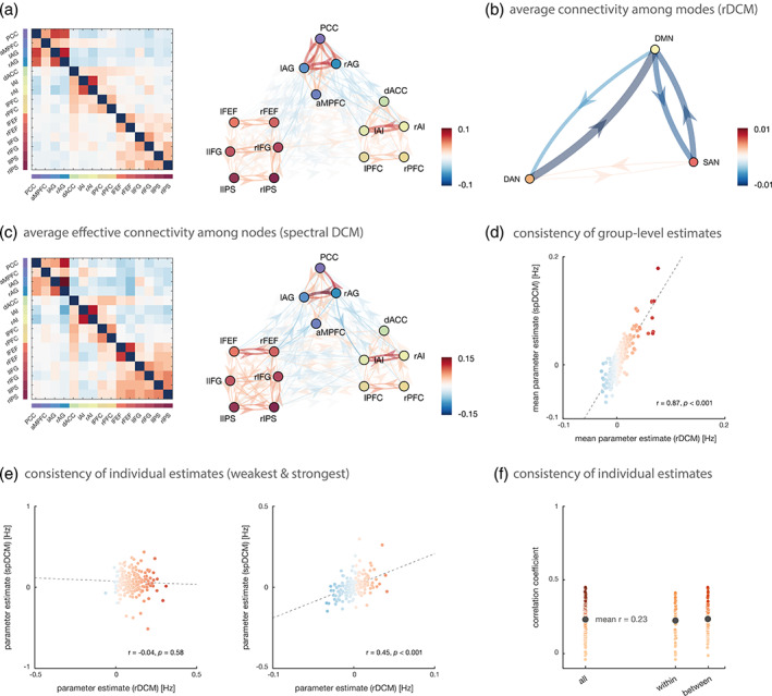
Effective connectivity among key brain regions of the resting state. (a) Group‐averaged posterior parameter estimates during the resting state as inferred with regression DCM (rDCM). (b) Average connection strength between resting‐state network (i.e., DMN, DAN, and SAN), computed as the average of the strength of all connections originating in one resting‐state network and terminating in another one. (c) Group‐averaged posterior parameter estimates during the resting state as inferred with spectral DCM (spDCM). Note that in order to make the correlation between group‐averaged connectivity estimates of the two DCM variants more easily visible, color was scaled in relation to the maximal values of each method. Hence, we utilize slightly different color scales for the two DCM variants for illustration purposes. (d) Consistency of group‐level parameter averages between rDCM and spDCM. Shown is the Pearson's correlation coefficient (r) among the group‐averaged inter‐regional connectivity estimates. Dots are colored using the rDCM color scale. (e) Consistency of individual parameter estimates for each connection separately; here, exemplarily shown for the connection with the weakest (left) and strongest association (right) between the two DCM variants. Dots are colored using the rDCM color scale. (f) Range of correlation coefficients across all 210 connections of the 15‐node network, as well as separately for all connections within a resting‐state network and all connections between resting‐state networks. Each colored dot represents the Pearson's correlation coefficient for an individual inter‐regional connection and the black dot denotes the mean Pearson's correlation coefficient, averaged across all connections. Note that averaging of individual Pearson's correlation coefficients was performed in z‐space (see main text)
In order to allow for direct comparability between this analysis of nodes and the previous analysis of modes, we computed the average connection strength between networks (Figure 5b). For example, the strength of all connections originating from a node of the DAN and terminating at a node of the DMN were averaged in order to yield the between‐network connection strength from the DAN to the DMN. This analysis suggested that, at the between‐network level, results from the 15‐node network were highly consistent with the ones obtained in the previous analysis of the 4‐mode network. Specifically, we again observed that the DMN was reciprocally connected to the other two RSNs via strong inhibitory connections, whereas the two task‐positive networks (i.e., DAN and SAN) showed excitatory coupling (although very weakly).
Finally, based on these between‐network connections (Figure 5b), we again computed the hierarchy strength as the difference between averaged absolute efferent and afferent connections between the three RSNs. As for the previous analysis, the total hierarchy strength was indicative of a hierarchical organization of the three networks with the DMN at the bottom (−0.007), predominantly serving as a sink, and the two task‐positive networks ranking higher (DAN: 0.006, SAN: 0.0007), predominantly serving as neuronal drivers. In fact, the three RSNs displayed even the exact same ordering as in the previous analysis of modes—a remarkable observation given the differences in the underlying networks—and are thus again consistent with previous work (Sridharan et al., 2008; Zhou et al., 2018).
3.3.2. Comparison to spectral DCM
As before, we compared our empirical findings from rDCM against the results obtained when utilizing spectral DCM to fit the identical BOLD signal time series. Group‐level effective connectivity patterns were again highly consistent across the two DCM variants (Figure 5c). Specifically, spectral DCM revealed the same modular structure of the (average) endogenous connectivity matrix with pronounced excitatory connections between regions of the same RSN and a more diverse pattern for between‐network connections. The similarity between the two DCM variants was again represented by a very high Pearson's correlation coefficient between the group‐level connectivity estimates (r = .87, p <.001; Figure 5d).
At the individual level, connections again varied in the degree of consistency between the two DCM variants. Correlations between rDCM and spectral DCM parameter estimates ranged from virtually absent (r = −.04, p = .58) for the connection from left to right IFG (Figure 5e, left) to robust (r = .45, p <.001) for the connection from left IPS to dACC (Figure 5e, right), representing a significant correlation. Overall, the mean correlation coefficient, averaged across all connections, was = .23 [.22 .24] (Figure 5f), and thus slightly decreased as compared to the 4‐mode networks. Nevertheless, consistency between rDCM and spectral DCM was significantly larger than zero, as assessed using a one‐sample t‐test (t [1,209] = 34.67, p <.001). Notably, consistency between the two DCM variants was not significantly different for within‐module as compared to between‐module connections (t [1,208] = −0.75, p = .46), suggesting that there was no systematic difference between those two types. As before, averaging of correlation coefficients as well as statistical testing were performed in z‐space—that is, after Fisher r‐to‐z transformation of the individual correlation coefficients.
In summary, these results were very similar to the ones obtained for the 4‐mode networks, although correlations at the individual level were overall somewhat lower for the 15‐node networks.
3.4. Empirical analysis: whole‐brain network
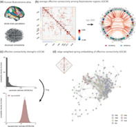
Having established the face validity and construct validity of rDCM for rs‐fMRI data in small networks, we assessed the practical utility of rDCM for inferring resting‐state effective connectivity at the whole‐brain level. To this end, we utilized the Brainnetome atlas as a whole‐brain parcellation scheme, using a 212‐node network covering the entire cortex (see Section 2 for details). Structural connectivity information provided by the Brainnetome atlas was used to constrain the network, resulting in 18,260 directed connections to be estimated (Figure 6a).
FIGURE 6.
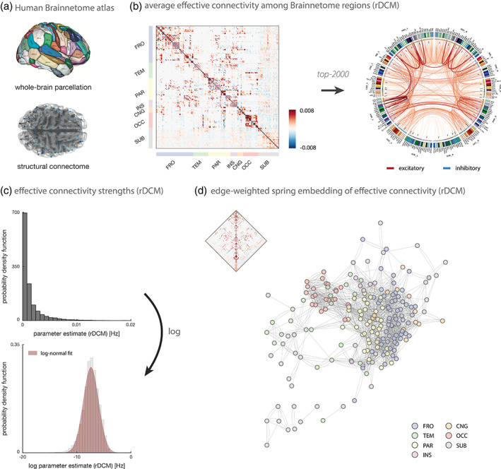
Whole‐brain effective connectivity during the resting state. (a) The whole‐brain rDCM analysis used the Human Brainnetome atlas that provides both a whole‐brain parcellation of cortical and subcortical regions as well as information on the structural connectivity among these parcels. The image of the Brainnetome parcellation was reprinted from Fan et al. (2016) with explicit permission from the copyright holder under the terms of the Creative commons attribution noncommercial license (http://creativecommons.org/licenses/by‐nc/4.0/). (b) Group‐averaged posterior estimates of directed connection strengths during the resting state as inferred with rDCM. Results are displayed as the full adjacency matrix (left) and as a connectogram of the top 2,000 connections with highest (absolute) weights (right). The connectogram was produced using Circos (publicly available at http://www.circos.ca/software/). Regions are divided into distinct sets, including frontal (FRO), temporal (TEM), parietal (PAR), insular (INS), cingulate (CNG; In the Brainnetome nomenclature, this set of regions is called “LIM” [limbic]. However, as the term “limbic” is not well‐defined (Kotter & Stephan, 1997) and since “LIM” exclusively consists of cingulate areas, we prefer to call this set of regions “CNG” [cingulate]), occipital (OCC), and subcortical (SUB). (c) Distribution of (absolute) endogenous connectivity parameters both in native (top) and logarithmic space (bottom). (d) Edge‐weighted spring embedding of the endogenous connectivity matrix based on the top 2,000 connections (see above). The edge‐weighted spring embedding projection was computed using Cytoscape (publicly available at https://cytoscape.org/download.html)
Applying rDCM to rs‐fMRI data from these 212 regions resulted in biologically plausible connectivity patterns (Figure 6b). The average endogenous connectivity matrix displayed a clear modular structure where regions within the same lobe (e.g., frontal, occipital) were strongly connected among each other (Figure 6b, left). Specifically, connections among regions within the same lobe were stronger and mostly positive (excitatory), whereas connections among regions in different lobes were more variable (i.e., showing both inhibitory and excitatory influences). This modular structure at the whole‐brain level is consistent with our analysis of the connectivity among resting‐state nodes. Furthermore, we found that while the majority of strong connections are within hemispheres, we also observed strong interhemispheric interactions, primarily among homotopic regions (Figure 6b, right).
Inspection of the distribution of (absolute) endogenous connectivity parameters revealed a log‐normal weight distribution, with connection strengths varying over several orders of magnitude (Figure 6c). This suggests a predominance of weak connections (corresponding to low‐frequency influences) in the average endogenous connectivity matrix. At the same time, the log‐normal distribution highlights the presence of an extended tail, indicating many strong connections (i.e., higher‐frequency influences) in the effective connectome. This finding is consistent with previous reports on log‐normal distributions of anatomical connection weights in the mouse cortex (Oh et al., 2014; Wang, Sporns, & Burkhalter, 2012) and in the macaque cortical connectome (Markov et al., 2013; Markov, Ercsey‐Ravasz, et al., 2014). The fall‐off from lower to higher frequency influences in the distribution of rDCM parameter estimates is also broadly consistent with the general spectral characteristics of rs‐fMRI data where low frequencies dominate (Chen & Glover, 2015; Kalcher et al., 2014; Niazy, Xie, Miller, Beckmann, & Smith, 2011).
Finally, the modular structure of the resting‐state effective connectivity becomes even more apparent when displaying the endogenous connectivity matrix as an edge‐weighted spring‐embedded projection. In brief, edge‐weighted spring embedding positions nodes that interact strongly next to each other, by treating each node as a steel ring linked by springs (edges), thereby forming a mechanical system (Kamada & Kawai, 1989). The optimal layout is then defined as one that minimizes the total energy of the system. Applying edge‐weighted spring embedding to the top 2000 connections of the average endogenous connectivity matrix revealed a clear modular structure with a tendency for nodes from the same set to cluster together (Figure 6d). This was particularly clear for regions in the occipital (red), parietal (yellow), and frontal lobe (blue). Furthermore, the spring‐embedded projection of the endogenous connectivity matrix was indicative of a hierarchical organization from occipital over parietal to frontal regions. This is consistent with the widespread view on brain organization as a hierarchy ranging from unimodal (e.g., visual) to transmodal (e.g., frontal) regions (Mesulam, 1998). Regions from some lobes (e.g., temporal) did not integrate clearly into this hierarchy, probably due to a dominance of weaker connection strengths below the chosen threshold. Notably, the spring‐embedded projection shown here should only be treated as a qualitative illustration, as the exact layout will depend on, for instance, the density of the network (and thus thresholding) and the exact initialization of the edge‐weighted spring embedding algorithm. Having said this, we verified that the overall pattern observed here holds for a range of different settings.
3.5. Computational burden
To provide an overview of computational efficiency, we report the run‐time for the different analyses. These values should be treated as a rough indication only, as run‐times will depend on the specific hardware used. Here, for all analyses, we used a single processor core on the Euler cluster at ETH Zurich (https://scicomp.ethz.ch/wiki/Euler).
First, rDCM took roughly 1 s for the small networks, regardless of the network architecture. More specifically, for the 4‐mode networks (16 free parameters: 12 connection and 4 inhibitory self‐connection parameters), model inversion took on average 0.48 ± 0.07 s (range: 0.35–0.77 s), whereas for the 15‐node networks (225 free parameters: 210 connection and 15 inhibitory self‐connection parameters), model inversion took on average 0.62 ± 0.10 s (range: 0.47–1.32 s). For the whole‐brain networks (18,260 free parameters: 18,048 connection and 212 inhibitory self‐connection parameters), model inversion took on average 132.30 ± 20.26 s (range: 90.63–175.30 s). This highlights the computational efficiency of rDCM in application to rs‐fMRI data and illustrates that the model scales gracefully with the number of regions, consistent with previous work on task‐fMRI (Frässle, Lomakina, et al., 2018; Frässle et al., 2017).
In comparison, while spectral DCM was also computationally efficient for the small networks, run‐times were considerably longer. Specifically, for the 4‐mode networks (30 free parameters: 12 connection, 4 inhibitory self‐connection, 6 hemodynamic, and 8 endogenous noise parameters), model inversion took on average 14.07 ± 5.99 s (range: 8.88–48.26 s), whereas for the 15‐node networks (261 free parameters: 210 connections, 15 inhibitory self‐connections, 17 hemodynamic, and 19 endogenous noise parameters), model inversion already took on average 3,031 ± 1,551s (range: 819–12,157 s).
In summary, although the number of free parameters of the small networks was comparable for the two DCM variants, run‐times were up to three orders of magnitude larger for spectral DCM. Specifically, our run‐time analyses suggest that rDCM scales much more gracefully to large networks as compared to spectral DCM. Here, we only applied rDCM to rs‐fMRI data from a parcellation with more than 200 areas; this was because runtimes of 21–42 hr per subject were reported for spectral DCM in application to a much smaller network of 36 regions (Razi et al., 2017).
4. DISCUSSION
In this article, we assessed the face validity and construct validity of regression DCM (rDCM; Frässle, Lomakina, et al., 2018; Frässle et al., 2017) for inferring effective connectivity during the resting state (i.e., unconstrained cognition) from noninvasive fMRI data. We demonstrated in simulation studies that rDCM can faithfully recover known model parameter values from synthetic rs‐fMRI data. Furthermore, we assessed the utility of rDCM in application to an empirical rs‐fMRI dataset acquired by the B‐SNIP‐1 consortium (Tamminga et al., 2013). These analyses suggest that rDCM yields biologically plausible results with regard to the functional integration during the resting state. Importantly, effective connectivity results obtained using rDCM in small networks (up to 15 nodes) were highly consistent with the estimates from spectral DCM when fitted to the identical BOLD signal time series. Furthermore, we then demonstrated that rDCM scales gracefully to large‐scale networks and provides sensible whole‐brain effective connectivity estimates from rs‐fMRI data within minutes.
First, we conducted comprehensive simulation studies to establish the face validity of rDCM when applied to synthetic resting‐state fMRI data. Specifically, we found that rDCM faithfully inferred upon the data‐generating (“true”) parameter values over a wide range of different settings of data quality (i.e., SNR) and sampling rate (i.e., TR). While model parameter recovery of rDCM improved for higher SNR and faster TR, consistent with previous observations in the context of task‐based fMRI (Frässle, Lomakina, et al., 2018; Frässle et al., 2017), performance was reasonable even for the most challenging scenario (i.e., SNR = 0.5, TR = 2 s). Besides this dependence on SNR and TR, model parameter recovery performance also depended on the complexity of the network with more accurate results being observed as the number of free parameters decreased.
Second, we applied rDCM to an empirical rs‐fMRI dataset to study the effective connectivity among entire RSNs (4 modes), as well as between their subcomponents (15 nodes). For both network architectures, results were biologically plausible and revealed inhibitory afferent and efferent connections for (regions of) the DMN, whereas (regions of) the task‐positive networks elicited predominantly excitatory coupling among each other. This was also represented by the fact that the different intrinsic RSNs followed a hierarchical ordering (under the given metric of hierarchy strength utilized in the present study), where the DMN was situated at the bottom (primarily serving as a sink) and the task‐positive networks (DAN, SAN, and CEN) were situated higher in the hierarchy (primarily serving as drivers). These findings were consistent with previous work on the hierarchical organization of RSNs (Sridharan et al., 2008; Zhou et al., 2018).
It is worth highlighting that several other studies have already applied DCM to resting‐state fMRI data and have found results consistent with observations reported here. Specifically, these studies have also demonstrated a tight functional coupling among regions within a given RSN (Razi et al., 2015; Zhou et al., 2018) as well as comparable patterns of integration between the RSNs (Zhou et al., 2018). This consistency is noteworthy given the substantial differences in analysis strategies among these studies. First, the generative model utilized ranged from regression DCM (present work) to spectral DCM (Razi et al., 2015; Sharaev, Zavyalova, Ushakov, Kartashov, & Velichkovsky, 2016; Zhou et al., 2018), stochastic DCM (Li, Wang, Yao, Hu, & Friston, 2012), and even deterministic DCM with a discrete cosine set (DCT) input (Di & Biswal, 2014). Second, studies differed in the exact choices made regarding preprocessing, the choice of regions/networks, and group level analyses. Despite these methodological and practical differences, all studies (including the present work) revealed tight coupling in the DMN between left angular gyrus and PCC, bilateral angular gyrus and the aMPFC, as well as reciprocal connections between left and right angular gyrus. In particular, the consistent involvement of the bilateral angular gyrus has been suggested to resemble its functional role in domain‐general automatic processing, where the angular gyrus has been claimed to function as an automatic bottom‐up buffer of incoming information (Humphreys & Lambon Ralph, 2017). Concerning functional integration among the subcomponents of the task‐positive networks, DCM studies have so far mainly focused on task‐based fMRI data. Nevertheless, these studies are still consistent with our findings in that pronounced integration was observed for regions of the SAN (Ham, Leff, de Boissezon, Joffe, & Sharp, 2013; Lamichhane & Dhamala, 2015) and DAN (Vossel, Weidner, Driver, Friston, & Fink, 2012).
Importantly, rDCM estimates were not only biologically plausible and consistent with previous findings in the literature, but also quantitatively similar to the results obtained using spectral DCM (Friston, Kahan, Biswal, & Razi, 2014). This is reassuring because spectral DCM represents a well‐established variant of DCM for resting‐state fMRI which has previously been tested in terms face validity (Friston, Kahan, Biswal, & Razi, 2014), construct validity (Razi et al., 2015), and test–retest reliability (Almgren et al., 2018). Hence, spectral DCM here served as a useful benchmark for assessing the construct validity of rDCM.
While group‐level estimates were highly consistent across the two variants of DCM, results were more variable at the individual level. Specifically, while individual parameter estimates were highly consistent for some connections, they were more variable between the two methods for others (Figures 4e and 5f). An interesting question for future work will be to disentangle whether the observed variability is merely due to chance or whether differences between the two methods for some of the connections actually represents meaningful differences in the variance that is picked up by rDCM and spectral DCM, respectively.
We would like to emphasize that, although rDCM and spectral DCM yielded comparable results for small networks (especially at the group level), rDCM was computationally much more efficient. This was indicated by run‐times that were up to three orders of magnitude higher for spectral DCM for the 15‐node network. While this increase in computational efficiency comes at the cost of physiological realism (e.g., fixed HRF, mean‐field approximation across regions), this allows rDCM to scale gracefully to very large networks with hundreds of brain regions. In contrast, the current implementation of spectral DCM is unlikely to scale to whole‐brain networks of this size, considering the run‐times reported here for the small networks as well as those reported previously, suggesting that model inversion of a single DCM with 36 regions takes between 21 and 42 hr (Razi et al., 2017).
Along these lines, we here conducted an additional exploratory analysis to demonstrate the practical feasibility of whole‐brain effective connectivity analyses during the resting state with rDCM. These analyses suggested that rDCM can indeed provide biologically plausible effective connectivity patterns at the whole‐brain level within minutes. Specifically, rDCM revealed an expected modular structure of the effective connectivity patterns, where areas of the same lobe grouped together and showed more pronounced within‐lobe interactions as compared to between‐lobe interactions. This is consistent with our findings on the coupling between components of the RSNs (“nodes”) as well as previous reports on functional integration during the resting state (Fornito, Zalesky, & Bullmore, 2016). Furthermore, (absolute) endogenous connection strengths inferred using rDCM followed a log‐normal distribution, consistent with previous reports on anatomical connection strengths in mice (Oh et al., 2014; Wang, Sporns, & Burkhalter, 2012) and macaques (Markov et al., 2013; Markov, Ercsey‐Ravasz, et al., 2014).
It is noteworthy that the average endogenous connection strengths for the whole‐brain network were an order of magnitude smaller than for the 4‐mode and 15‐node networks. This is a consequence of the choice of priors utilized in rDCM. More specifically, in rDCM, the variance of the shrinkage prior scales with ~1/N, where N is the number of regions. This choice of prior variance is identical to the one utilized for classical DCMs in SPM and aims to counteract the problem of overfitting which increases with the number of regions (and thus the number of connections and free parameters). In other words, by making the prior variance dependent on the number of regions, we regularize the estimates of individual connection strengths in a manner that grows with the size of the network. In the current study, the range of estimated connection strengths for the whole‐brain model is comparable to those reported in a previous publication that demonstrated the construct validity of the model for task‐based fMRI data (Frässle et al., 2021).
The combination of computational efficiency and applicability to simple conditions like the “resting state” renders rDCM particularly promising for application in the fields of Computational Psychiatry and Computational Neurology. Here, computational readouts of directed connectivity in whole‐brain networks are of major relevance because global dysconnectivity has been postulated as a hallmark of most psychiatric and neurological disorders (Deco & Kringelbach, 2014; Fornito et al., 2015; Frässle, Yao, et al., 2018; Menon, 2011; Stephan, Iglesias, Heinzle, & Diaconescu, 2015). The ability to infer whole‐brain effective connectivity patterns from rs‐fMRI measurements is appealing from a clinical perspective as it puts minimal burden on the patient in the MR scanner. Besides these promises for clinical applications, computational efficiency, and application to rs‐fMRI renders rDCM also a promising tool for analyses of large‐scale datasets (Sudlow et al., 2015; Van Essen et al., 2013). These datasets typically focus on rs‐fMRI for its advantage in terms of easy harmonization of multi‐site acquisition efforts. The vast amount of data available from these consortia calls for computational tools that are highly efficient. We anticipate that the application of rDCM to these open‐source datasets may represent an exciting new opportunity to move human connectomics and network neuroscience towards directed measures of functional integration.
It is worth mentioning that, while we replicated previous findings on putative anticorrelations between the task‐negative network (DMN) and the task‐positive networks (DAN, SAN) during the resting state (Fox et al., 2005), one should be cautious with regard to the interpretation of this finding. Specifically, it has been argued that the observed anticorrelations may—at least in part—be a consequence of specific preprocessing choices. In particular, global signal regression has been argued to artificially induce anticorrelations by removing any positive correlation between DMN and DAN/SAN that may be hidden in the signal (Buckner et al., 2008; Fox et al., 2009; Murphy, Birn, Handwerker, Jones, & Bandettini, 2009). In the present work, we did perform global signal regression to correct for potential confounds like psychological, hardware, and motion artifacts. Hence, results obtained with rDCM in the present study are consistent with previous reports that followed comparable preprocessing strategies (e.g., global signal regression). However, our methodological study cannot—and does not intend—to resolve the ongoing controversy on the validity of anticorrelations between RSNs.
Finally, we would like to highlight that the development of rDCM is still in an early stage and the present implementation is subject to several limitations. First, in its current form, rDCM does not account for variability in the hemodynamic response across regions and subjects (Aguirre, Zarahn, & D'esposito, 1998; Handwerker, Ollinger, & D'Esposito, 2004). In this study, using simulated fMRI data with realistic hemodynamic variability across regions, rDCM proved to be surprisingly robust and even allowed for superior connectivity parameter recovery compared to spectral DCM (Figure 3), a model that does account for region‐specific hemodynamics. Nevertheless, a major future development is to replace the fixed HRF with a more flexible hemodynamic model that still preserves the computational efficiency of rDCM.
Second, it is worth emphasizing that—although rDCM performs well in practice (both in simulations and empirical applications)—the approach presented in this article should only be seen as an initial pragmatic solution to enable application of rDCM to the resting state. This is because the generative model of rDCM does not represent endogenous fluctuations in neuronal activity explicitly. Instead, endogenous fluctuations of BOLD signal in any given region are explained, in the frequency domain, as a linear mixture of intrinsic fluctuations in other regions. This rests on the fact that the measured (instead of predicted) data enters the design matrix in Equation (1). This formulation effectively renders rDCM similar to a multivariate autoregressive model in the frequency domain (compare Frässle et al., 2017). While this works well in practice for both task (Frässle, Lomakina, et al., 2018; Frässle et al., 2017, 2021) and resting‐state data, this represents an important conceptual limitation of rDCM since this removes the strict separation between (latent) state and (measured) observation levels that is otherwise a characteristic feature of DCMs. Consequently, another major future development for rDCM is to explicitly account for endogenous neuronal fluctuations in the generative forward model and re‐separate state from observation levels.
Third, the linear formulation of rDCM and the stationarity assumption of the Fourier transform implies that only stationary measures of functional integration can be obtained. However, functional integration changes dynamically on short timescales, under the influence of synaptic plasticity and neuromodulation (Stephan et al., 2015). Models of effective connectivity in the context of task fMRI data have long accounted for this nonstationarity by considering dynamic changes in connectivity as a function of cognitive context (Friston et al., 2003) or local activity (Stephan et al., 2008). More recently, research on the resting state has also recognized the importance of time‐varying functional integration for a more comprehensive understanding of the organizing principles of the human brain; this constitutes an active area of research (e.g., Chang & Glover, 2010; Hutchison et al., 2013; Lurie et al., 2020; Preti, Bolton, & Van De Ville, 2017; Vidaurre et al., 2017). These studies have highlighted the reoccurring nature of dynamic functional connectivity patterns and proposed descriptions that model states of functional connectivity as attractor states in a high dimensional space (Vergara et al., 2020). Furthermore, alterations in the dynamics of functional integration during the resting state have been linked to a number of psychiatric and neurological conditions, including schizophrenia (Rashid, Damaraju, Pearlson, & Calhoun, 2014; Sakoglu et al., 2010), depression (Kaiser et al., 2016), autism (de Lacy, Doherty, King, Rachakonda, & Calhoun, 2017), Parkinson's (Diez‐Cirarda et al., 2018), and Alzheimer's disease (Jones et al., 2012). Hence, a major goal for future developments of our approach will be to introduce dynamics to the effective connectivity estimates obtained with rDCM.
Despite these limitations, our results demonstrate the face and construct validity of rDCM for modeling rs‐fMRI data: they demonstrate good recovery of known connection strengths from simulated data, illustrate that rDCM can infer biologically plausible effective connectivity patterns from empirical rs‐fMRI data and show that rDCM estimates are consistent with results from spectral DCM, a well‐established DCM variant for rs‐fMRI. Importantly, due to the computational efficiency of our method, rDCM scales gracefully with network size and provides sensible whole‐brain resting‐state effective connectivity patterns. This opens up promising new avenues for whole‐brain connectomics based on directed measures of functional integration during the resting state. Such a readout of whole‐brain effective connectivity will hopefully not only provide novel insights into the organizing principles of the human brain in health, but might also prove valuable for unraveling pathophysiological mechanisms and for enabling single‐subject predictions about clinical outcomes (Frässle et al., 2020).
CONFLICT OF INTEREST
The authors declare no potential conflict of interest.
DATA AVAILABILITY STATEMENT
A Matlab implementation of the regression dynamic causal modeling (rDCM) approach is available as open source code in the Translational Algorithms for Psychiatry‐Advancing Science (TAPAS) toolbox (www.translationalneuromodeling.org/tapas). Extensions to the rDCM toolbox that facilitate its application to rs‐fMRI data have already been made available. Furthermore, following acceptance of this article, we will publish the code for the analysis as well as the source data files for figures and tables online as part of an online repository that conforms to the FAIR (Findable, Accessible, Interoperable, and Re‐usable) data principles. Additionally, the raw data acquired by the B‐SNIP‐1 consortium is openly available from the NIMH RDoC database (RDoCdb; https://nda.nih.gov) which also conforms to the FAIR principles.
Supporting information
Appendix S1: Supporting Information
ACKNOWLEDGMENTS
This work was supported by the UZH Forschungskredit Postdoc (Stefan Frässle), the ETH Zurich Postdoctoral Fellowship Program and the Marie Curie Actions for People COFUND Program (Stefan Frässle), the Strategic Focal Area “Personalized Health and Related Technologies (PHRT)” of the ETH Domain grant #2017‐403 (Samuel J. Harrison), the René and Susanne Braginsky Foundation (Klaas E. Stephan), the Swiss National Science Foundation 320030_179377 (Klaas E. Stephan), and the University of Zurich (Klaas E. Stephan). Open Access funding enabled and organized by ProjektDEAL.
Frässle S, Harrison SJ, Heinzle J, et al. Regression dynamic causal modeling for resting‐state fMRI. Hum Brain Mapp. 2021;42:2159–2180. 10.1002/hbm.25357
Funding information ETH Zurich Postdoctoral Fellowship Program and the Marie Curie Actions for People COFUND Program, Grant/Award Number: FEL‐49 15‐2; René and Susanne Braginsky Foundation; Schweizerischer Nationalfonds zur Förderung der Wissenschaftlichen Forschung, Grant/Award Number: 320030_179377; Strategic Focal Area “Personalized Health and Related Technologies (PHRT)” of the ETH Domain, Grant/Award Number: 2017‐403; Universität Zürich; UZH Forschungskredit Postdoc, Grant/Award Number: FK‐18‐046
REFERENCES
- Aguirre, G. K. , Zarahn, E. , & D'esposito, M. (1998). The variability of human, BOLD hemodynamic responses. NeuroImage, 8, 360–369. [DOI] [PubMed] [Google Scholar]
- Almgren, H. , Van de Steen, F. , Kuhn, S. , Razi, A. , Friston, K. , & Marinazzo, D. (2018). Variability and reliability of effective connectivity within the core default mode network: A multi‐site longitudinal spectral DCM study. NeuroImage, 183, 757–768. [DOI] [PMC free article] [PubMed] [Google Scholar]
- Andreasen, N. C. , Endicott, J. , Spitzer, R. L. , & Winokur, G. (1977). The family history method using diagnostic criteria: Reliability and validity. Archives of General Psychiatry, 34, 1229–1235. [DOI] [PubMed] [Google Scholar]
- Avants, B. B. , Epstein, C. L. , Grossman, M. , & Gee, J. C. (2008). Symmetric diffeomorphic image registration with cross‐correlation: evaluating automated labeling of elderly and neurodegenerative brain. Medical Image Analysis, 12, 26–41. [DOI] [PMC free article] [PubMed] [Google Scholar]
- Baker, J. T. , Dillon, D. G. , Patrick, L. M. , Roffman, J. L. , Brady, R. O., Jr. , Pizzagalli, D. A. , … Holmes, A. J. (2019). Functional connectomics of affective and psychotic pathology. Proceedings of the National Academy of Sciences of the United States of America, 116, 9050–9059. [DOI] [PMC free article] [PubMed] [Google Scholar]
- Baker, J. T. , Holmes, A. J. , Masters, G. A. , Yeo, B. T. , Krienen, F. , Buckner, R. L. , & Ongur, D. (2014). Disruption of cortical association networks in schizophrenia and psychotic bipolar disorder. JAMA Psychiatry, 71, 109–118. [DOI] [PMC free article] [PubMed] [Google Scholar]
- Bassett, D. S. , & Sporns, O. (2017). Network neuroscience. Nature Neuroscience, 20, 353–364. [DOI] [PMC free article] [PubMed] [Google Scholar]
- Beckmann, C. F. , DeLuca, M. , Devlin, J. T. , & Smith, S. M. (2005). Investigations into resting‐state connectivity using independent component analysis. Philosophical Transactions of the Royal Society B‐Biological Sciences, 360, 1001–1013. [DOI] [PMC free article] [PubMed] [Google Scholar]
- Bishop, C. M. (2006). Pattern recognition and machine learning. New York: Springer; 12, 13, 47, 105. [Google Scholar]
- Biswal, B. , Yetkin, F. Z. , Haughton, V. M. , & Hyde, J. S. (1995). Functional connectivity in the motor cortex of resting human brain using echo‐planar MRI. Magnetic Resonance in Medicine, 34, 537–541. [DOI] [PubMed] [Google Scholar]
- Biswal, B. B. , Van Kylen, J. , & Hyde, J. S. (1997). Simultaneous assessment of flow and BOLD signals in resting‐state functional connectivity maps. NMR in Biomedicine, 10, 165–170. [DOI] [PubMed] [Google Scholar]
- Buckholtz, J. W. , & Meyer‐Lindenberg, A. (2012). Psychopathology and the human connectome: Toward a transdiagnostic model of risk for mental illness. Neuron, 74, 990–1004. [DOI] [PubMed] [Google Scholar]
- Buckner, R. L. , Andrews‐Hanna, J. R. , & Schacter, D. L. (2008). The brain's default network: anatomy, function, and relevance to disease. Annals of the New York Academy of Sciences, 1124, 1–38. [DOI] [PubMed] [Google Scholar]
- Bullmore, E. , & Sporns, O. (2009). Complex brain networks: Graph theoretical analysis of structural and functional systems. Nature Reviews. Neuroscience, 10, 186–198. [DOI] [PubMed] [Google Scholar]
- Chang, C. , & Glover, G. H. (2010). Time‐frequency dynamics of resting‐state brain connectivity measured with fMRI. NeuroImage, 50, 81–98. [DOI] [PMC free article] [PubMed] [Google Scholar]
- Chen, J. E. , & Glover, G. H. (2015). BOLD fractional contribution to resting‐state functional connectivity above 0.1 Hz. NeuroImage, 107, 207–218. [DOI] [PMC free article] [PubMed] [Google Scholar]
- Corbetta, M. , & Shulman, G. L. (2002). Control of goal‐directed and stimulus‐driven attention in the brain. Nature Reviews. Neuroscience, 3, 201–215. [DOI] [PubMed] [Google Scholar]
- Courchesne, E. , Pierce, K. , Schumann, C. M. , Redcay, E. , Buckwalter, J. A. , Kennedy, D. P. , & Morgan, J. (2007). Mapping early brain development in autism. Neuron, 56, 399–413. [DOI] [PubMed] [Google Scholar]
- Craddock, R. C. , Jbabdi, S. , Yan, C. G. , Vogelstein, J. T. , Castellanos, F. X. , Di Martino, A. , … Milham, M. P. (2013). Imaging human connectomes at the macroscale. Nature Methods, 10, 524–539. [DOI] [PMC free article] [PubMed] [Google Scholar]
- Daunizeau, J. , Friston, K. , & Kiebel, S. (2009). Variational Bayesian identification and prediction of stochastic nonlinear dynamic causal models. Physica D‐Nonlinear Phenomena, 238, 2089–2118. [DOI] [PMC free article] [PubMed] [Google Scholar]
- de Lacy, N. , Doherty, D. , King, B. H. , Rachakonda, S. , & Calhoun, V. D. (2017). Disruption to control network function correlates with altered dynamic connectivity in the wider autism spectrum. NeuroImage: Clinical, 15, 513–524. [DOI] [PMC free article] [PubMed] [Google Scholar]
- Deco, G. , & Kringelbach, M. L. (2014). Great expectations: using whole‐brain computational connectomics for understanding neuropsychiatric disorders. Neuron, 84, 892–905. [DOI] [PubMed] [Google Scholar]
- Di, X. , & Biswal, B. B. (2014). Modulatory interactions between the default mode network and task positive networks in resting‐state. PeerJ, 2, e367. [DOI] [PMC free article] [PubMed] [Google Scholar]
- Diez‐Cirarda, M. , Strafella, A. P. , Kim, J. , Pena, J. , Ojeda, N. , Cabrera‐Zubizarreta, A. , & Ibarretxe‐Bilbao, N. (2018). Dynamic functional connectivity in Parkinson's disease patients with mild cognitive impairment and normal cognition. NeuroImage: Clinical, 17, 847–855. [DOI] [PMC free article] [PubMed] [Google Scholar]
- Dosenbach, N. U. , Fair, D. A. , Miezin, F. M. , Cohen, A. L. , Wenger, K. K. , Dosenbach, R. A. , … Petersen, S. E. (2007). Distinct brain networks for adaptive and stable task control in humans. Proceedings of the National Academy of Sciences of the United States of America, 104, 11073–11078. [DOI] [PMC free article] [PubMed] [Google Scholar]
- Esteban, O. , Birman, D. , Schaer, M. , Koyejo, O. O. , Poldrack, R. A. , & Gorgolewski, K. J. (2017). MRIQC: Advancing the automatic prediction of image quality in MRI from unseen sites. PLoS One, 12, e0184661. [DOI] [PMC free article] [PubMed] [Google Scholar]
- Esteban, O. , Markiewicz, C. J. , Blair, R. W. , Moodie, C. A. , Isik, A. I. , Erramuzpe, A. , … Gorgolewski, K. J. (2019). fMRIPrep: A robust preprocessing pipeline for functional MRI. Nature Methods, 16, 111–116. [DOI] [PMC free article] [PubMed] [Google Scholar]
- Fan, L. , Li, H. , Zhuo, J. , Zhang, Y. , Wang, J. , Chen, L. , … Jiang, T. (2016). The human brainnetome atlas: A new brain atlas based on connectional architecture. Cerebral Cortex, 26, 3508–3526. [DOI] [PMC free article] [PubMed] [Google Scholar]
- Felleman, D. J. , & Van Essen, D. C. (1991). Distributed hierarchical processing in the primate cerebral cortex. Cerebral Cortex, 1, 1–47. [DOI] [PubMed] [Google Scholar]
- Fonov, V. , Evans, A. , McKinstry, R. , Almli, C. R. , & Collins, D. (2009). Unbiased nonlinear average age‐appropriate brain templates from birth to adulthood. NeuroImage, 47, S102. [Google Scholar]
- Fornito, A. , Zalesky, A. , Bassett, D. S. , Meunier, D. , Ellison‐Wright, I. , Yucel, M. , … Bullmore, E. T. (2011). Genetic influences on cost‐efficient organization of human cortical functional networks. The Journal of Neuroscience, 31, 3261–3270. [DOI] [PMC free article] [PubMed] [Google Scholar]
- Fornito, A. , Zalesky, A. , & Breakspear, M. (2015). The connectomics of brain disorders. Nature Reviews. Neuroscience, 16, 159–172. [DOI] [PubMed] [Google Scholar]
- Fornito, A. , Zalesky, A. , & Bullmore, E. (2016). Fundamentals of Brain Network Analysis, London, England: Elsevier Inc. [Google Scholar]
- Fox, M. D. , Corbetta, M. , Snyder, A. Z. , Vincent, J. L. , & Raichle, M. E. (2006). Spontaneous neuronal activity distinguishes human dorsal and ventral attention systems. Proceedings of the National Academy of Sciences of the United States of America, 103, 10046–10051. [DOI] [PMC free article] [PubMed] [Google Scholar]
- Fox, M. D. , & Raichle, M. E. (2007). Spontaneous fluctuations in brain activity observed with functional magnetic resonance imaging. Nature Reviews. Neuroscience, 8, 700–711. [DOI] [PubMed] [Google Scholar]
- Fox, M. D. , Snyder, A. Z. , Vincent, J. L. , Corbetta, M. , Van Essen, D. C. , & Raichle, M. E. (2005). The human brain is intrinsically organized into dynamic, anticorrelated functional networks. Proceedings of the National Academy of Sciences of the United States of America, 102, 9673–9678. [DOI] [PMC free article] [PubMed] [Google Scholar]
- Fox, M. D. , Zhang, D. , Snyder, A. Z. , & Raichle, M. E. (2009). The global signal and observed anticorrelated resting state brain networks. Journal of Neurophysiology, 101, 3270–3283. [DOI] [PMC free article] [PubMed] [Google Scholar]
- Frässle, S. , Lomakina, E. I. , Kasper, L. , Manjaly, Z. M. , Leff, A. , Pruessmann, K. P. , … Stephan, K. E. (2018). A generative model of whole‐brain effective connectivity. NeuroImage, 179, 505–529. [DOI] [PubMed] [Google Scholar]
- Frässle, S. , Lomakina, E. I. , Razi, A. , Friston, K. J. , Buhmann, J. M. , & Stephan, K. E. (2017). Regression DCM for fMRI. NeuroImage, 155, 406–421. [DOI] [PubMed] [Google Scholar]
- Frässle, S. , Manjaly, Z. M. , Do, C. T. , Kasper, L. , Pruessmann, K. P. , & Stephan, K. E. (2021). Whole‐brain estimates of directed connectivity for human connectomics. NeuroImage, 225, 117491. [DOI] [PubMed] [Google Scholar]
- Frässle, S. , Marquand, A. F. , Schmaal, L. , Dinga, R. , Veltman, D. J. , van der Wee, N. J. A. , … Stephan, K. E. (2020). Predicting individual clinical trajectories of depression with generative embedding. NeuroImage: Clinical, 26, 102213. [DOI] [PMC free article] [PubMed] [Google Scholar]
- Frässle, S. , Paulus, F. M. , Krach, S. , Schweinberger, S. R. , Stephan, K. E. , & Jansen, A. (2016). Mechanisms of hemispheric lateralization: Asymmetric interhemispheric recruitment in the face perception network. NeuroImage, 124, 977–988. [DOI] [PubMed] [Google Scholar]
- Frässle, S. , Yao, Y. , Schöbi, D. , Aponte, E. A. , Heinzle, J. , & Stephan, K. E. (2018). Generative models for clinical applications in computational psychiatry. Wiley Interdisciplinary Reviews: Cognitive Science, 9, e1460. [DOI] [PubMed] [Google Scholar]
- Friston, K. , Brown, H. R. , Siemerkus, J. , & Stephan, K. E. (2016). The dysconnection hypothesis (2016). Schizophrenia Research, 176, 83–94. [DOI] [PMC free article] [PubMed] [Google Scholar]
- Friston, K. , Harrison, L. , & Penny, W. (2003). Dynamic causal modelling. NeuroImage, 19, 1273–1302. [DOI] [PubMed] [Google Scholar]
- Friston, K. , Mattout, J. , Trujillo‐Barreto, N. , Ashburner, J. , & Penny, W. (2007). Variational free energy and the Laplace approximation. NeuroImage, 34, 220–234. [DOI] [PubMed] [Google Scholar]
- Friston, K. J. (2011). Functional and effective connectivity: a review. Brain Connectivity, 1, 13–36. [DOI] [PubMed] [Google Scholar]
- Friston, K. J. , Kahan, J. , Biswal, B. , & Razi, A. (2014). A DCM for resting state fMRI. NeuroImage, 94, 396–407. [DOI] [PMC free article] [PubMed] [Google Scholar]
- Friston, K. J. , Kahan, J. , Razi, A. , Stephan, K. E. , & Sporns, O. (2014). On nodes and modes in resting state fMRI. NeuroImage, 99, 533–547. [DOI] [PMC free article] [PubMed] [Google Scholar]
- Friston, K. J. , Williams, S. , Howard, R. , Frackowiak, R. S. , & Turner, R. (1996). Movement‐related effects in fMRI time‐series. Magnetic Resonance in Medicine, 35, 346–355. [DOI] [PubMed] [Google Scholar]
- Gazzaniga, M. S. (2000). Cerebral specialization and interhemispheric communication: Does the corpus callosum enable the human condition? Brain, 123(Pt 7), 1293–1326. [DOI] [PubMed] [Google Scholar]
- Glahn, D. C. , Winkler, A. M. , Kochunov, P. , Almasy, L. , Duggirala, R. , Carless, M. A. , … Blangero, J. (2010). Genetic control over the resting brain. Proceedings of the National Academy of Sciences of the United States of America, 107, 1223–1228. [DOI] [PMC free article] [PubMed] [Google Scholar]
- Gorgolewski, K. , Burns, C. D. , Madison, C. , Clark, D. , Halchenko, Y. O. , Waskom, M. L. , & Ghosh, S. S. (2011). Nipype: a flexible, lightweight and extensible neuroimaging data processing framework in python. Frontiers in Neuroinformatics, 5, 13. [DOI] [PMC free article] [PubMed] [Google Scholar]
- Goulas, A. , Uylings, H. B. , & Stiers, P. (2014). Mapping the hierarchical layout of the structural network of the macaque prefrontal cortex. Cerebral Cortex, 24, 1178–1194. [DOI] [PubMed] [Google Scholar]
- Greicius, M. D. , Flores, B. H. , Menon, V. , Glover, G. H. , Solvason, H. B. , Kenna, H. , … Schatzberg, A. F. (2007). Resting‐state functional connectivity in major depression: abnormally increased contributions from subgenual cingulate cortex and thalamus. Biological Psychiatry, 62, 429–437. [DOI] [PMC free article] [PubMed] [Google Scholar]
- Greicius, M. D. , Supekar, K. , Menon, V. , & Dougherty, R. F. (2009). Resting‐state functional connectivity reflects structural connectivity in the default mode network. Cerebral Cortex, 19, 72–78. [DOI] [PMC free article] [PubMed] [Google Scholar]
- Greve, D. N. , & Fischl, B. (2009). Accurate and robust brain image alignment using boundary‐based registration. NeuroImage, 48, 63–72. [DOI] [PMC free article] [PubMed] [Google Scholar]
- Hahamy, A. , Behrmann, M. , & Malach, R. (2015). The idiosyncratic brain: distortion of spontaneous connectivity patterns in autism spectrum disorder. Nature Neuroscience, 18, 302–309. [DOI] [PubMed] [Google Scholar]
- Ham, T. , Leff, A. , de Boissezon, X. , Joffe, A. , & Sharp, D. J. (2013). Cognitive control and the salience network: An investigation of error processing and effective connectivity. The Journal of Neuroscience, 33, 7091–7098. [DOI] [PMC free article] [PubMed] [Google Scholar]
- Handwerker, D. A. , Ollinger, J. M. , & D'Esposito, M. (2004). Variation of BOLD hemodynamic responses across subjects and brain regions and their effects on statistical analyses. NeuroImage, 21, 1639–1651. [DOI] [PubMed] [Google Scholar]
- Hilgetag, C. C. , & Goulas, A. (2020). Hierarchy' in the organization of brain networks. Philosophical Transactions of the Royal Society of London. Series B, Biological Sciences, 375, 20190319. [DOI] [PMC free article] [PubMed] [Google Scholar]
- Humphreys, G. F. , & Lambon Ralph, M. A. (2017). Mapping domain‐selective and counterpointed domain‐general higher cognitive functions in the lateral parietal cortex: Evidence from fMRI comparisons of difficulty‐varying semantic versus visuo‐spatial tasks, and functional connectivity analyses. Cerebral Cortex, 27, 4199–4212. [DOI] [PubMed] [Google Scholar]
- Hutchison, R. M. , Womelsdorf, T. , Allen, E. A. , Bandettini, P. A. , Calhoun, V. D. , Corbetta, M. , … Chang, C. (2013). Dynamic functional connectivity: Promise, issues, and interpretations. NeuroImage, 80, 360–378. [DOI] [PMC free article] [PubMed] [Google Scholar]
- Jenkinson, M. , Bannister, P. , Brady, M. , & Smith, S. (2002). Improved optimization for the robust and accurate linear registration and motion correction of brain images. NeuroImage, 17, 825–841. [DOI] [PubMed] [Google Scholar]
- Jenkinson, M. , Beckmann, C. F. , Behrens, T. E. , Woolrich, M. W. , & Smith, S. M. (2012). Fsl. NeuroImage, 62, 782–790. [DOI] [PubMed] [Google Scholar]
- Jenkinson, M. , & Smith, S. (2001). A global optimisation method for robust affine registration of brain images. Medical Image Analysis, 5, 143–156. [DOI] [PubMed] [Google Scholar]
- Jones, D. T. , Vemuri, P. , Murphy, M. C. , Gunter, J. L. , Senjem, M. L. , Machulda, M. M. , … Jack, C. R., Jr. (2012). Non‐stationarity in the "resting brain's" modular architecture. PLoS One, 7, e39731. [DOI] [PMC free article] [PubMed] [Google Scholar]
- Kaiser, R. H. , Whitfield‐Gabrieli, S. , Dillon, D. G. , Goer, F. , Beltzer, M. , Minkel, J. , … Pizzagalli, D. A. (2016). Dynamic Resting‐State Functional Connectivity in Major Depression. Neuropsychopharmacology, 41, 1822–1830. [DOI] [PMC free article] [PubMed] [Google Scholar]
- Kalcher, K. , Boubela, R. N. , Huf, W. , Bartova, L. , Kronnerwetter, C. , Derntl, B. , … Moser, E. (2014). The spectral diversity of resting‐state fluctuations in the human brain. PLoS One, 9, e93375. [DOI] [PMC free article] [PubMed] [Google Scholar]
- Kamada, T. , & Kawai, S. (1989). An algorithm for drawing general undirected graphs. Information Processing Letters, 31, 7–15. [Google Scholar]
- Karahanoglu, F. I. , & Van De Ville, D. (2017). Dynamics of large‐scale fMRI networks: Deconstruct brain activity to build better models of brain function. Current Opinion in Biomedical Engineering, 3, 28–36. [Google Scholar]
- Kotter, R. , & Stephan, K. E. (1997). Useless or helpful? The "limbic system" concept. Reviews in the Neurosciences, 8, 139–145. [DOI] [PubMed] [Google Scholar]
- Lamichhane, B. , & Dhamala, M. (2015). The salience network and its functional architecture in a perceptual decision: An effective connectivity study. Brain Connectivity, 5, 362–370. [DOI] [PubMed] [Google Scholar]
- Li, B. , Daunizeau, J. , Stephan, K. E. , Penny, W. , Hu, D. , & Friston, K. (2011). Generalised filtering and stochastic DCM for fMRI. NeuroImage, 58, 442–457. [DOI] [PubMed] [Google Scholar]
- Li, B. J. , Wang, X. , Yao, S. Q. , Hu, D. W. , & Friston, K. J. (2012). Task‐dependent modulation of effective connectivity within the default mode network. Frontiers in Psychology, 3, 206. [DOI] [PMC free article] [PubMed] [Google Scholar]
- Lui, S. , Yao, L. , Xiao, Y. , Keedy, S. K. , Reilly, J. L. , Keefe, R. S. , … Sweeney, J. A. (2015). Resting‐state brain function in schizophrenia and psychotic bipolar probands and their first‐degree relatives. Psychological Medicine, 45, 97–108. [DOI] [PMC free article] [PubMed] [Google Scholar]
- Lurie, D. J. , Kessler, D. , Bassett, D. S. , Betzel, R. F. , Breakspear, M. , Kheilholz, S. , … Calhoun, V. D. (2020). Questions and controversies in the study of time‐varying functional connectivity in resting fMRI. Network Neuroscience, 4, 30–69. [DOI] [PMC free article] [PubMed] [Google Scholar]
- Markov, N. T. , Ercsey‐Ravasz, M. , Van Essen, D. C. , Knoblauch, K. , Toroczkai, Z. , & Kennedy, H. (2013). Cortical high‐density counterstream architectures. Science, 342, 1238406. [DOI] [PMC free article] [PubMed] [Google Scholar]
- Markov, N. T. , Ercsey‐Ravasz, M. M. , Ribeiro Gomes, A. R. , Lamy, C. , Magrou, L. , Vezoli, J. , … Kennedy, H. (2014). A weighted and directed interareal connectivity matrix for macaque cerebral cortex. Cerebral Cortex, 24, 17–36. [DOI] [PMC free article] [PubMed] [Google Scholar]
- Markov, N. T. , Vezoli, J. , Chameau, P. , Falchier, A. , Quilodran, R. , Huissoud, C. , … Kennedy, H. (2014). Anatomy of hierarchy: feedforward and feedback pathways in macaque visual cortex. The Journal of Comparative Neurology, 522, 225–259. [DOI] [PMC free article] [PubMed] [Google Scholar]
- Menon, V. (2011). Large‐scale brain networks and psychopathology: A unifying triple network model. Trends in Cognitive Sciences, 15, 483–506. [DOI] [PubMed] [Google Scholar]
- Menon, V. , & Uddin, L. Q. (2010). Saliency, switching, attention and control: a network model of insula function. Brain Structure & Function, 214, 655–667. [DOI] [PMC free article] [PubMed] [Google Scholar]
- Mesulam, M. M. (1998). From sensation to cognition. Brain, 121(Pt 6), 1013–1052. [DOI] [PubMed] [Google Scholar]
- Mortamet, B. , Bernstein, M. A. , Jack, C. R., Jr. , Gunter, J. L. , Ward, C. , Britson, P. J. , … Alzheimer's Disease Neuroimaging Initiative . (2009). Automatic quality assessment in structural brain magnetic resonance imaging. Magnetic Resonance in Medicine, 62, 365–372. [DOI] [PMC free article] [PubMed] [Google Scholar]
- Murphy, K. , Birn, R. M. , Handwerker, D. A. , Jones, T. B. , & Bandettini, P. A. (2009). The impact of global signal regression on resting state correlations: are anti‐correlated networks introduced? NeuroImage, 44, 893–905. [DOI] [PMC free article] [PubMed] [Google Scholar]
- Nee, D. E. , & D'Esposito, M. (2016). The hierarchical organization of the lateral prefrontal cortex. eLife, 5, 1–26. [DOI] [PMC free article] [PubMed] [Google Scholar]
- Niazy, R. K. , Xie, J. , Miller, K. , Beckmann, C. F. , & Smith, S. M. (2011). Spectral characteristics of resting state networks. Progress in Brain Research, 193, 259–276. [DOI] [PubMed] [Google Scholar]
- Oh, S. W. , Harris, J. A. , Ng, L. , Winslow, B. , Cain, N. , Mihalas, S. , … Zeng, H. (2014). A mesoscale connectome of the mouse brain. Nature, 508, 207–214. [DOI] [PMC free article] [PubMed] [Google Scholar]
- Picchioni, D. , Duyn, J. H. , & Horovitz, S. G. (2013). Sleep and the functional connectome. NeuroImage, 80, 387–396. [DOI] [PMC free article] [PubMed] [Google Scholar]
- Power, J. D. , Barnes, K. A. , Snyder, A. Z. , Schlaggar, B. L. , & Petersen, S. E. (2012). Spurious but systematic correlations in functional connectivity MRI networks arise from subject motion. NeuroImage, 59, 2142–2154. [DOI] [PMC free article] [PubMed] [Google Scholar]
- Power, J. D. , Mitra, A. , Laumann, T. O. , Snyder, A. Z. , Schlaggar, B. L. , & Petersen, S. E. (2014). Methods to detect, characterize, and remove motion artifact in resting state fMRI. NeuroImage, 84, 320–341. [DOI] [PMC free article] [PubMed] [Google Scholar]
- Preti, M. G. , Bolton, T. A. , & Van De Ville, D. (2017). The dynamic functional connectome: State‐of‐the‐art and perspectives. NeuroImage, 160, 41–54. [DOI] [PubMed] [Google Scholar]
- Raichle, M. E. (2015). The brain's default mode network. Annual Review of Neuroscience, 38, 433–447. [DOI] [PubMed] [Google Scholar]
- Raichle, M. E. , MacLeod, A. M. , Snyder, A. Z. , Powers, W. J. , Gusnard, D. A. , & Shulman, G. L. (2001). A default mode of brain function. Proceedings of the National Academy of Sciences of the United States of America, 98, 676–682. [DOI] [PMC free article] [PubMed] [Google Scholar]
- Rashid, B. , Damaraju, E. , Pearlson, G. D. , & Calhoun, V. D. (2014). Dynamic connectivity states estimated from resting fMRI Identify differences among Schizophrenia, bipolar disorder, and healthy control subjects. Frontiers in Human Neuroscience, 8, 897. [DOI] [PMC free article] [PubMed] [Google Scholar]
- Razi, A. , Kahan, J. , Rees, G. , & Friston, K. J. (2015). Construct validation of a DCM for resting state fMRI. NeuroImage, 106, 1–14. [DOI] [PMC free article] [PubMed] [Google Scholar]
- Razi, A. , Seghier, M. L. , Zhou, Y. , McColgan, P. , Zeidman, P. , Park, H. J. , … Friston, K. J. (2017). Large‐scale DCMs for resting‐state fMRI. Network Neuroscience, 1, 222–241. [DOI] [PMC free article] [PubMed] [Google Scholar]
- Sakoglu, U. , Pearlson, G. D. , Kiehl, K. A. , Wang, Y. M. , Michael, A. M. , & Calhoun, V. D. (2010). A method for evaluating dynamic functional network connectivity and task‐modulation: Application to schizophrenia. Magma, 23, 351–366. [DOI] [PMC free article] [PubMed] [Google Scholar]
- Satterthwaite, T. D. , Elliott, M. A. , Gerraty, R. T. , Ruparel, K. , Loughead, J. , Calkins, M. E. , … Wolf, D. H. (2013). An improved framework for confound regression and filtering for control of motion artifact in the preprocessing of resting‐state functional connectivity data. NeuroImage, 64, 240–256. [DOI] [PMC free article] [PubMed] [Google Scholar]
- Sharaev, M. G. , Zavyalova, V. V. , Ushakov, V. L. , Kartashov, S. I. , & Velichkovsky, B. M. (2016). Effective connectivity within the default mode network: dynamic causal modeling of resting‐state fMRI data. Frontiers in Human Neuroscience, 10, 14. [DOI] [PMC free article] [PubMed] [Google Scholar]
- Shirer, W. R. , Ryali, S. , Rykhlevskaia, E. , Menon, V. , & Greicius, M. D. (2012). Decoding subject‐driven cognitive states with whole‐brain connectivity patterns. Cerebral Cortex, 22, 158–165. [DOI] [PMC free article] [PubMed] [Google Scholar]
- Shulman, G. L. , Fiez, J. A. , Corbetta, M. , Buckner, R. L. , Miezin, F. M. , Raichle, M. E. , & Petersen, S. E. (1997). Common Blood Flow Changes across Visual Tasks: II. Decreases in Cerebral Cortex. Journal of Cognitive Neuroscience, 9, 648–663. [DOI] [PubMed] [Google Scholar]
- Smith, S. M. , Fox, P. T. , Miller, K. L. , Glahn, D. C. , Fox, P. M. , Mackay, C. E. , … Beckmann, C. F. (2009). Correspondence of the brain's functional architecture during activation and rest. Proceedings of the National Academy of Sciences of the United States of America, 106, 13040–13045. [DOI] [PMC free article] [PubMed] [Google Scholar]
- Smith, S. M. , Vidaurre, D. , Beckmann, C. F. , Glasser, M. F. , Jenkinson, M. , Miller, K. L. , … Van Essen, D. C. (2013). Functional connectomics from resting‐state fMRI. Trends in Cognitive Sciences, 17, 666–682. [DOI] [PMC free article] [PubMed] [Google Scholar]
- Spreng, R. N. (2012). The fallacy of a "task‐negative" network. Frontiers in Psychology, 3, 145. [DOI] [PMC free article] [PubMed] [Google Scholar]
- Spreng, R. N. , Sepulcre, J. , Turner, G. R. , Stevens, W. D. , & Schacter, D. L. (2013). Intrinsic architecture underlying the relations among the default, dorsal attention, and frontoparietal control networks of the human brain. Journal of Cognitive Neuroscience, 25, 74–86. [DOI] [PMC free article] [PubMed] [Google Scholar]
- Spreng, R. N. , Stevens, W. D. , Chamberlain, J. P. , Gilmore, A. W. , & Schacter, D. L. (2010). Default network activity, coupled with the frontoparietal control network, supports goal‐directed cognition. NeuroImage, 53, 303–317. [DOI] [PMC free article] [PubMed] [Google Scholar]
- Sridharan, D. , Levitin, D. J. , & Menon, V. (2008). A critical role for the right fronto‐insular cortex in switching between central‐executive and default‐mode networks. Proceedings of the National Academy of Sciences of the United States of America, 105, 12569–12574. [DOI] [PMC free article] [PubMed] [Google Scholar]
- Stam, C. J. (2014). Modern network science of neurological disorders. Nature Reviews. Neuroscience, 15, 683–695. [DOI] [PubMed] [Google Scholar]
- Stephan, K. , Kasper, L. , Harrison, L. , Daunizeau, J. , den Ouden, H. , Breakspear, M. , & Friston, K. (2008). Nonlinear dynamic causal models for fMRI. NeuroImage, 42, 649–662. [DOI] [PMC free article] [PubMed] [Google Scholar]
- Stephan, K. , Marshall, J. , Penny, W. , Friston, K. , & Fink, G. (2007). Interhemispheric integration of visual processing during task‐driven lateralization. The Journal of Neuroscience, 27, 3512–3522. [DOI] [PMC free article] [PubMed] [Google Scholar]
- Stephan, K. E. , Iglesias, S. , Heinzle, J. , & Diaconescu, A. O. (2015). Translational perspectives for computational neuroimaging. Neuron, 87, 716–732. [DOI] [PubMed] [Google Scholar]
- Sudlow, C. , Gallacher, J. , Allen, N. , Beral, V. , Burton, P. , Danesh, J. , … Collins, R. (2015). UK biobank: An open access resource for identifying the causes of a wide range of complex diseases of middle and old age. PLoS Medicine, 12, e1001779. [DOI] [PMC free article] [PubMed] [Google Scholar]
- Tagliazucchi, E. , & Laufs, H. (2014). Decoding wakefulness levels from typical fMRI resting‐state data reveals reliable drifts between wakefulness and sleep. Neuron, 82, 695–708. [DOI] [PubMed] [Google Scholar]
- Tamminga, C. A. , Ivleva, E. I. , Keshavan, M. S. , Pearlson, G. D. , Clementz, B. A. , Witte, B. , … Sweeney, J. A. (2013). Clinical phenotypes of psychosis in the Bipolar‐Schizophrenia network on intermediate phenotypes (B‐SNIP). The American Journal of Psychiatry, 170, 1263–1274. [DOI] [PMC free article] [PubMed] [Google Scholar]
- Tamminga, C. A. , Pearlson, G. , Keshavan, M. , Sweeney, J. , Clementz, B. , & Thaker, G. (2014). Bipolar and schizophrenia network for intermediate phenotypes: outcomes across the psychosis continuum. Schizophrenia Bulletin, 40(Suppl 2), S131–S137. [DOI] [PMC free article] [PubMed] [Google Scholar]
- Treiber, J. M. , White, N. S. , Steed, T. C. , Bartsch, H. , Holland, D. , Farid, N. , … Chen, C. C. (2016). Characterization and correction of geometric distortions in 814 diffusion weighted images. PLoS One, 11, e0152472. [DOI] [PMC free article] [PubMed] [Google Scholar]
- Tustison, N. J. , Avants, B. B. , Cook, P. A. , Zheng, Y. , Egan, A. , Yushkevich, P. A. , & Gee, J. C. (2010). N4ITK: improved N3 bias correction. IEEE Transactions on Medical Imaging, 29, 1310–1320. [DOI] [PMC free article] [PubMed] [Google Scholar]
- van den Heuvel, M. P. , & Hulshoff Pol, H. E. (2010). Exploring the brain network: A review on resting‐state fMRI functional connectivity. European Neuropsychopharmacology, 20, 519–534. [DOI] [PubMed] [Google Scholar]
- Van Essen, D. C. , Smith, S. M. , Barch, D. M. , Behrens, T. E. J. , Yacoub, E. , Ugurbil, K. , & Consortium, W.‐M. H. (2013). The WU‐Minn Human Connectome Project: An overview. NeuroImage, 80, 62–79. [DOI] [PMC free article] [PubMed] [Google Scholar]
- Vergara, V. M. , van der Horn, J. H. , Mayer, A. R. , Espinoza, F. A. , van der Naalt, J. , Calhoun, V. D. (2020). Mild traumatic brain injury disrupts functional dynamic attractors of healthy mental states. doi: 10.1101/19007906. [DOI]
- Vidaurre, D. , Abeysuriya, R. , Becker, R. , Quinn, A. J. , Alfaro‐Almagro, F. , Smith, S. M. , & Woolrich, M. W. (2017). Discovering dynamic brain networks from big data in rest and task. NeuroImage. 180, 646–656. [DOI] [PMC free article] [PubMed] [Google Scholar]
- Vossel, S. , Weidner, R. , Driver, J. , Friston, K. J. , & Fink, G. R. (2012). Deconstructing the architecture of dorsal and ventral attention systems with dynamic causal modeling. The Journal of Neuroscience, 32, 10637–10648. [DOI] [PMC free article] [PubMed] [Google Scholar]
- Wang, L. , Hermens, D. F. , Hickie, I. B. , & Lagopoulos, J. (2012). A systematic review of resting‐state functional‐MRI studies in major depression. Journal of Affective Disorders, 142, 6–12. [DOI] [PubMed] [Google Scholar]
- Wang, Q. , Sporns, O. , & Burkhalter, A. (2012). Network analysis of corticocortical connections reveals ventral and dorsal processing streams in mouse visual cortex. The Journal of Neuroscience, 32, 4386–4399. [DOI] [PMC free article] [PubMed] [Google Scholar]
- Wang, S. , Peterson, D. J. , Gatenby, J. C. , Li, W. , Grabowski, T. J. , & Madhyastha, T. M. (2017). Evaluation of field map and nonlinear registration methods for correction of susceptibility artifacts in diffusion MRI. Frontiers in Neuroinformatics, 11, 17. [DOI] [PMC free article] [PubMed] [Google Scholar]
- Zeki, S. , & Shipp, S. (1988). The functional logic of cortical connections. Nature, 335, 311–317. [DOI] [PubMed] [Google Scholar]
- Zhang, Y. , Brady, M. , & Smith, S. (2001). Segmentation of brain MR images through a hidden Markov random field model and the expectation‐maximization algorithm. IEEE Transactions on Medical Imaging, 20, 45–57. [DOI] [PubMed] [Google Scholar]
- Zhou, Y. , Friston, K. J. , Zeidman, P. , Chen, J. , Li, S. , & Razi, A. (2018). The hierarchical organization of the default, dorsal attention and salience networks in adolescents and young adults. Cerebral Cortex, 28, 726–737. [DOI] [PMC free article] [PubMed] [Google Scholar]
Associated Data
This section collects any data citations, data availability statements, or supplementary materials included in this article.
Supplementary Materials
Appendix S1: Supporting Information
Data Availability Statement
A Matlab implementation of the regression dynamic causal modeling (rDCM) approach is available as open source code in the Translational Algorithms for Psychiatry‐Advancing Science (TAPAS) toolbox (www.translationalneuromodeling.org/tapas). Extensions to the rDCM toolbox that facilitate its application to rs‐fMRI data have already been made available. Furthermore, following acceptance of this article, we will publish the code for the analysis as well as the source data files for figures and tables online as part of an online repository that conforms to the FAIR (Findable, Accessible, Interoperable, and Re‐usable) data principles. Additionally, the raw data acquired by the B‐SNIP‐1 consortium is openly available from the NIMH RDoC database (RDoCdb; https://nda.nih.gov) which also conforms to the FAIR principles.