Quantile Regression Forests to Identify Determinants of Neighborhood Stroke Prevalence in 500 Cities in the USA: Implications for Neighborhoods with High Prevalence

Abstract

Stroke exerts a massive burden on the US health and economy. Place-based evidence is increasingly recognized as a critical part of stroke management, but identifying the key determinants of neighborhood stroke prevalence and the underlying effect mechanisms is a topic that has been treated sparingly in the literature. We aim to fill in the research gaps with a study focusing on urban health. We develop and apply analytical approaches to address two challenges. First, domain expertise on drivers of neighborhood-level stroke outcomes is limited. Second, commonly used linear regression methods may provide incomplete and biased conclusions. We created a new neighborhood health data set at census tract level by pooling information from multiple sources. We developed and applied a machine learning–based quantile regression method to uncover crucial neighborhood characteristics for neighborhood stroke outcomes among vulnerable neighborhoods burdened with high prevalence of stroke. Neighborhoods with a larger share of non-Hispanic blacks, older adults, or people with insufficient sleep tended to have a higher prevalence of stroke, whereas neighborhoods with a higher socio-economic status in terms of income and education had a lower prevalence of stroke. The effects of five major determinants varied geographically and were significantly stronger among neighborhoods with high prevalence of stroke. Highly flexible machine learning identifies true drivers of neighborhood cardiovascular health outcomes from wide-ranging information in an agnostic and reproducible way. The identified major determinants and the effect mechanisms can provide important avenues for prioritizing and allocating resources to develop optimal community-level interventions for stroke prevention.

Background

Stroke is the fifth leading cause of death in the USA and is a major cause of serious disability for adults [1]. The prevalence of stroke is approximately 3%, accounting for one of every 20 deaths. With an estimated $45.5 billion in direct and indirect costs, stroke is a chronic disease exerting a massive burden on the US health and economy. Considerable research has been conducted on the risk factors for stroke at the individual level [2–4]. These studies have demonstrated accumulative scientific evidence showing that stroke is associated with modifiable risk factors, such as high blood pressure, obesity, and high cholesterol, and health behavioral risk factors, such as smoking, sleep deprivation, and sedentary lifestyle [5–8]. There are also remarkable disparities, with higher stroke incidence and prevalence found among older population, Blacks, and those with low socioeconomic status [9].

In comparison, few studies have examined the mechanisms between neighborhood characteristics and neighborhood-level prevalence of stroke, despite the growing awareness that individuals’ health is closely related to the neighborhood environment they live in [10, 11]. The connections between place and health can be seen in the apparent clustering of high prevalence of stroke in the Stroke Belt states and in certain census tracts across major US cities [12, 13]. However, there is an insufficient understanding of what and how neighborhood characteristics drive the neighborhood-level prevalence of stroke. Identifying critical predictors is important as it provides an opportunity for policymakers to plan tailored community-based interventions, which have been shown to be more effective and cost-effective in reducing the burden of cardiovascular disease and curbing health care costs compared with individual-based interventions [14].

This study aims to contribute to neighborhood cardiovascular health research. We address two primary challenges. First, in public health research, domain expertise is frequently used for variable selection. However, subject matter expertise on key drivers of neighborhood-level cardiovascular health outcomes and their relative importance is limited. In practice, variable selection is often carried out with certain degree of arbitrariness (e.g., tests based on statistical significance level, the order in which variables are entered into a model, the choice of a statistical model). In addition, the relative importance of each variable in relation to the outcome is often unclear.

Second, commonly used linear regression (LR) methods for determining the association between exposures and an outcome assess how the mean of the conditional distribution of the outcome varies with exposures. However, the mean of the neighborhood-level prevalence of stroke may be a poor indicator of central tendency and conveys limited information about how prevalence of stroke varies across different neighborhoods. The distribution of the neighborhood-level prevalence of stroke is skewed; see Fig. 1. The effect of a factor may be different across quantiles. Consequently, using LR methods to estimate only the effects at the mean level may result in incomplete and biased conclusion about the effect.

Fig. 1.

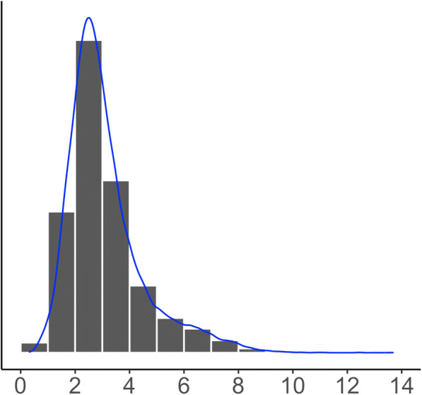
Distribution of the neighborhood-level prevalence of stroke is right skewed. Skewness = 1.5 and kurtosis = 6.0

Research is needed to understand the most important links between neighborhood-level characteristics and a high prevalence of stroke at the neighborhood level, as such knowledge would aid in prioritizing and deploying prevention interventions for the affected communities. Focusing on these vulnerable communities requires an analysis of the tail of a distribution, e.g., 90th percentile of the distribution of the prevalence of stroke as it signals “troubled” neighborhoods.

Quantile regression (QR) methods are well suited to estimate how specified quantiles or percentiles of the distribution of the outcome variable vary with covariates and is robust against outliers and is more informative for a skewed distribution than mean-based regression [15, 16]. In this article, we demonstrate the value of a highly flexible machine learning–based quantile regression method in studying neighborhood stroke burden.

We first created a large-scale neighborhood health data by pooling information from multiple sources and considered 24 factors. These factors have been linked to cardiovascular health outcomes at the individual patient level and can be grouped into four major domains, unhealthy behaviors, prevention measures, sociodemographic indicators, and environmental measures [5, 6, 8, 9]. We then exploited quantile regression forests (QRFs)—a machine learning modeling technique—to rank the relative importance of the potential predictors and proposed and implemented an algorithm to identify a set of major determinants for the distribution of neighborhood-level prevalence of stroke. We further compared the performance of our machine learning method to the performance of regression approaches commonly used in practice. Finally, we quantified the effects of the identified major determinants on stroke prevalence in vulnerable neighborhoods where the stroke prevalence ranked in the 90th percentile and assessed the bias from mean-based analyses.

Results from this study will provide insights into how to prioritize and incorporate the fabric of neighborhood health and sociodemographic environment into stroke-prevention strategies for communities heavily burdened with stroke.

Methods

We created a new neighborhood health data set by pooling information in three datasets from the Centers for Disease Control and Prevention (CDC), the Census Bureau, and the Environmental Protection Agency (EPA) in the USA. Census tract was used as a proxy of neighborhood. Data on the prevalence of health outcomes, prevention, and health behavior measures were drawn from the CDC’s 500 Cities Project 2017 data release on 28,004 census tracts [17]. The project was funded by the Robert Wood Johnson Foundation in conjunction with the CDC Foundation. Socio-demographic measures for the selected census tracts were from the 2011–2015 American Community Survey 5-Year Estimates [18, 19]. Information on environmental exposures was obtained from the EPA’s Environmental Justice Screening (EJSCREEN) database [20]. We did not obtain IRB approval as this ecological study used census tract level data from publicly available data sources.

We included four types of neighborhood risk factors: (i) unhealthy behaviors (e.g., smoking, no leisure-time physical activity, insufficient sleep, and obesity), (ii) prevention measures (e.g., lack of health insurance, visits to dentist, colonoscopy screening, up to date on a core set of preventative services for male and females), (iii) sociodemographic indicators (e.g., age, sex, race/ethnicity, income, and education), and (iv) environmental measures (e.g., ambient air pollution). Both the stroke outcome and its predictor variables were measured at the neighborhood level (no person-level data were used). Detailed description of the variables and their data sources and distributions are shown in Table 1. We excluded 1307 census tracts that had missing data on key variables. Among the 1307 census tracts, 975 had missing health measures, 137 had missing socio-demographic measures, and 295 had missing environmental data. Our final analytical dataset included 26,697 census tracts.

Table 1.

Distribution of 24 potential neighborhood-level predictors and prevalence of stroke across 500 cities. Measures are in percentages for all variables except those marked with an asterisk

Domain	Variable name	Definition	Min	Q1	Median	Q3	Max	Mean	Data source
Health outcomes	STROKE	Stroke among adults aged ≥ 18 years	0.30	2.20	2.80	3.60	18.80	3.11	CDC 500 Cities Data
Unhealthy behaviors	SMOKING	Current smoking among adults aged ≥ 18 years	2.00	14.30	18.30	23.10	48.70	19.10	CDC 500 Cities Dataa
	NO_PA	No leisure-time physical activity among adults aged ≥ 18 years	7.90	18.30	24.20	31.60	61.30	25.30
	OBESITY	Obesity among adults aged ≥ 18 years	8.70	23.70	28.60	34.90	58.50	29.76
	INSUF_SLEEP	Sleeping less than 7 h among adults aged ≥ 18 years	18.50	32.50	36.30	41.20	59.80	37.10
Prevention	LACK_INSURANCE	Current lack of health insurance among adults aged 18–64 years	2.50	11.70	18.00	27.40	70.80	20.58	CDC 500 Cities Data
	DENTAL	Visits to dentist or dental clinic among adults aged ≥ 18 years	18.90	49.80	61.30	70.50	87.10	59.82
	COLON_SCREEN	Fecal occult blood test, sigmoidoscopy, or colonoscopy among adults aged 50–75 years	23.40	52.60	60.60	66.60	81.50	59.29
	CORE_PREV_M	Older adults aged ≥ 65 years who are up to date on a core set of clinical preventive services (men: flu shot past year, pneumococcal polysaccharides vaccine (PPV) shot ever, colorectal cancer screening)	13.10	24.80	29.90	34.60	52.20	29.88
	CORE_PREV_W	Older adults aged ≥ 65 years who are up to date on a core set of clinical preventive services (women: same as above and mammogram past 2 years)	9.60	23.00	28.60	33.90	53.80	28.64
Socio-demographic status	AGE65_OVER	Population aged 65 and over	0.00	10.61	14.81	19.79	100.00	15.81	ACSb
	AGE18_34	Population aged between 18 and 34	0.00	27.48	33.78	40.76	99.38	34.96
	COLLEGE_HIGHER	Bachelor’s degree or higher	0.00	12.27	23.71	40.33	100.00	28.28
	HS_COLLEGE	High school graduate or higher	0.00	75.78	85.51	91.66	100.00	82.44
	FEMALE	Female	0.00	48.82	51.19	53.60	100.00	51.04
	NON_HIS_ASIAN	Not Hispanic or Latino: Asian alone	0.00	0.72	3.08	8.50	91.32	7.26
	NON_HIS_BLACK	Not Hispanic or Latino: Black or African American alone	0.00	2.19	7.37	24.43	100.00	19.73
	NON_HIS_OTHER	Not Hispanic or Latino: Other	0.00	2.07	4.61	8.06	50.70	6.02
	NON_HIS_WHITE	Not Hispanic or Latino: White alone	0.00	17.24	48.02	72.15	100.00	45.65
	POVERTY	Below poverty level; estimate; families	0.00	5.10	12.10	24.00	100.00	16.09
	MED_INCOME*	Median household income in the past 12 months (in thousands)	4.17	34.10	49.58	70.43	250.00	55.49
Environmental factors	HOUSE_PRE1960*	Pre-1960 housing (lead paint indicator) (in thousands)	0.00	0.10	0.48	0.92	8.13	0.59
	TRAFFIC*	Traffic proximity and volume (average number of vehicles/distance)	0.00	0.12	0.39	1.10	62.11	11.73
	OZONE*	Ozone level in air (ppb)	27.63	44.40	48.74	52.81	73.67	48.04	EPA-EJSCREENc
	PM25*	PM2.5 level in air (μg/m3)	4.97	8.54	9.89	10.66	13.32	9.71

PM_2.5 concentrations are annual average of the daily ambient average, and ozone concentrations are average of daily maximum 8-h level for the summer season. Both PM_2.5 and ozone were from a space-time downscaling fusion model based on monitoring data and modeled data. Traffic data reflect annual average daily traffic count of vehicles, i.e., count of vehicle at major roads within 500 m divided by distance in meters, and was calculated based on traffic data from the US Department of Transportation. Pre-1960 housing data were based on ACS from the US Census

*Variables with absolute measurements as opposed to percentages

^aCensus tract level 500 Cities Data from the Centers for Disease Control and Prevention (CDC), which were modeled based on population-based survey data from the Behavioral Risk Factor Surveillance System (BRFSS)

^bCensus tract level data from the 2011–2015 American Community Survey 5-Year Estimates provided by the Census Bureau

^cTo match the geospatial unit of census tract available in the other two data sources, we aggregated the census block group level environmental measures to the census tract level by taking the means for PM_2.5 and O₃ and the sum for the housing data and the sum of block-group-level population weighted traffic data

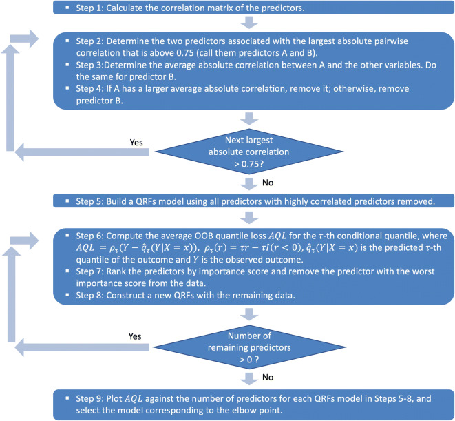
We first explored a heuristic approach to remove the minimum number of highly correlated predictor variables. Redundant predictors add complexity to the model than information they provide to the model. Using highly correlated predictors in regression models can lead to highly unstable results. The variance inflation factor (VIF) can be used to identify predictors that are impacted but does not determine which should be removed to resolve the problem. We followed an iterative algorithm to remove the minimum number of variables to ensure that all pairwise correlations are below a certain threshold, for which we chose 0.75 [21]. Details of the algorithm appear in Fig. 2.

Fig. 2.

Variable selection algorithm using quantile regression forests

We then applied a high-performance nonparametric machine learning technique, QRFs, on the reduced data with no highly correlated variables. QRFs is a generalization of the random forests (RFs). RFs are a machine learning modeling technique that builds an ensemble of regression trees to flexibly capture the relationship between the conditional mean of the response and predictor variables and has gained popularity in medical research for its high prediction accuracy and adaptability [22–24]. QRFs utilizes the infrastructure of RFs and gives a nonparametric and accurate way of estimating conditional quantiles. The method has been shown to be consistent and competitive in terms of predictive power [25]. QRFs grows an ensemble of regression trees, employing random nodes and split point selection as in the standard RFs algorithm, but for each node in each tree, RFs keeps only the mean of the observations that fall into this node, whereas QRFs keeps the values of all observations in the node. Thus, QRFs can assess the conditional distribution function of the response given the covariates and can provide a fuller picture of the exposure-outcome relationship than mean-based RFs.

We developed and implemented a variable selection algorithm based on the variable importance scores generated by QRFs to determine the most critical predictors for the 90th percentile of the neighborhood-level prevalence rate of stroke. The algorithm is described in Fig. 2. A similar algorithm was suggested by Dietrich et al. for implementing RFs with survival outcomes but without assessing the optimal balance between the prediction error and the number of selected variables [26]. The importance score for each variable is computed by randomly permuting the values of each predictor for the out-of-bag (OOB) sample of the predictor for each tree and measuring the decrease in model accuracy by the permutation averaged across the forest. The more important the variable is, the larger decrease (i.e., importance score) is produced by the permutation. We carried out an iterative process for variable selection. Each time, we removed the least important variable and rebuilt a QRFs model with the remaining variables and recorded the OOB average quantile loss (AQL) until no variable is left. We used AQL for the evaluation of model performance because the true conditional quantiles of the responses are unobservable. So as suggested by Wang et al. and Fang et al., we computed the prediction error of the τth conditional quantile by averaging the quantile loss function, ${\rho }_{\tau }\left(Y-{\widehat{q}}_{\tau }\left(Y|X=x\right)\right)$, overall observations, where ρ_τ(r) = τr − rI(r < 0) [27, 28]. We then plotted the OOB AQLs against the number of selected variables and set the final model to be the one corresponding to the “elbow” point, which achieved the best balance between the smallest OOB AQL and the parsimoniousness of the selected variables.

To empirically evaluate whether our machine learning algorithm selected major determinants, we compared QRFs with classical linear QR including all predictors additively, termed as LQR-AllVar, which is frequently used in public health. To demonstrate the benefit of our first step of removing highly correlated variables, we applied our variable selection algorithm using QRFs to the full set of 24 predictors, and we termed this approach as QRFs-F. We compared the metric AQL and AQL reduction per predictor—defined as (AQL_null − AQL_method)/Number of Predictors_method, where AQL_null is the AQL from the null model, i.e., intercept only model, and AQL_method corresponds to the AQL of each method. AQL reduction per predictor answers the question of how much gain do we get for adding each predictor variable suggested by a variable selection approach, and therefore methods that give larger AQL reduction per predictor are desired.

Finally, to “unblackbox” machine learning, we included the major predictors selected by QRFs in a linear QR model to quantify the effects of each predictor on different percentiles of the response and in an LR model to show how mean-based analysis may provide incomplete and biased summary of the effect of exposures. All statistical analyses were performed using R version 3.6.1. QRF models were built using the “quantregForest” R package.

Results

We first applied the iterative algorithm (steps 1–4 in Fig. 2) to identify and remove 8 redundant and highly correlated variables from the 24 candidate predictors. We then built a QRFs model with the remaining16 predictors and ranked the relative importance of each predictor in relation to the 90th percentile of the neighborhood-level prevalence of stroke; see Fig. 3. Sociodemographic indicators related to race, age, income level, education, and unhealthy sleep behavior appeared to be the leading neighborhood-level risk factors for high prevalence of stroke, whereas the environmental measures and gender composition are of relatively low importance.

Fig. 3.

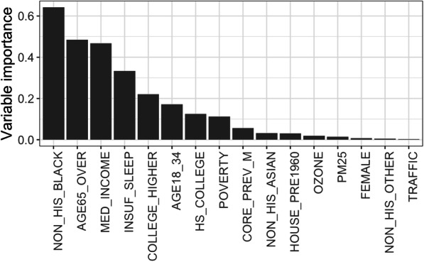
Importance ranking of predictors for the neighborhood-level prevalence of stroke based on 10,000 trained trees for the QRFs. Importance is measured as follows. For each tree, the prediction performance (i.e., mean squared errors) on the OOB samples is recorded. Then the values of each predictor in the OOB samples are randomly permuted, and the prediction performance based on the shuffled data is recorded. The importance score of that variable is measured as decrease in the prediction performance after permutation averaged across all trees. QRFs quantile regression forests, OOB out-of-bag

We further identified major determinants of high stroke prevalence using the relative importance scores. Targeting the 90th percentile of the prevalence of stroke at the neighborhood level, our QRFs-based variable selection algorithm (steps 5–9 in Fig. 2) identified five crucial factors that explained the majority of the variability in stroke prevalence among the most vulnerable neighborhoods. They are, in the order of relative importance, the share of non-Hispanic blacks, the proportion the percentage of population over 65 years of age, median household income, the percentage of population with insufficient sleep, and the share of population with higher education. These five predictors correspond to the “elbow” point in Fig. 4—variables remained in the QRFs model in the 11th iteration of our QRFs variable selection algorithm. Together, the predictors reduced the AQL from the null model (with no predictors) by 70%, similar to the percentage of reduction in AQL (72.5%) delivered by a full model including all 16 available predictors, as suggested in Fig. 4 by the curve of OOB AQL gradually reaching a plateau after the “elbow” point. The AQL reduction per predictor achieved by these five predictors was 0.04 as compared with 0.01 by the full model.

Fig. 4.

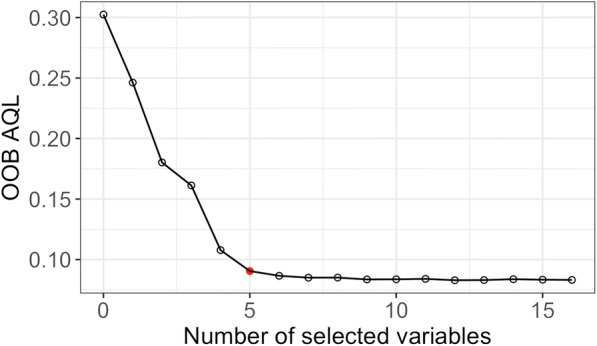
Estimated out-of-bag average quantile loss for the 90th percentile corresponding to each iteration in our QRFs variable selection algorithm. The red dot indicates the “elbow” point, at which the optimal balance between model accuracy and parsimoniousness of the selected variables is achieved. QRFs quantile regression forests

Figure 5 compares the performances of QRFs, QRFs-F, and LQR-AllVar in terms of the prediction error of the 90th quantile, number of selected variables, and prediction error reduction per predictor. While QRFs distinguished only five factors out of 16 available factors, the machine learning–based method gave a similar AQL as LQR-AllVar did for predicting the 90th percentile of the neighborhood-level prevalence of stroke and obtained a significantly larger error reduction per predictor. The AQL from QRFs-F was the same as that from QRFs. Consequently, the QRFs-F method yielded a smaller AQL reduction per predictor; see Table 2. In addition, several variables selected via QRFs-F were highly correlated (results not shown). For example, the Pearson correlation coefficient was − 0.92 between the proportion of people who have dental insurance and the proportion of people who have no leisure-time physical activity and 0.83 between the proportion of obese people and the proportion of people who have no leisure-time physical activity. These results showed that the presence of highly correlated predictors may adversely impact QRFs’ ability to identify strong predictors [29] and that QRFs may be sensitive to selecting highly correlated and redundant predictors. The findings corroborated that our method identified true determinants. We further investigated whether the better performance of QRFs over LQR-AllVar was due to the possible nonlinear covariate–outcome relationships and interactions among predictors. Figure 6 shows the partial dependence functions between the outcome and the five identified key determinants, demonstrating the marginal effects of the five determinants on the 90th percentile of the neighborhood-level prevalence of stroke. The marginal effects were nonlinear for median household income, the proportion of people who are above 65, and the proportion of people with insufficient sleep. The interaction measures based on the normalized minimal depth of variable [30] indicate that the interactions among these five key determinants were quite substantial (results not shown).

Fig. 5.

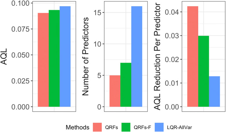
Comparison of QRFs, QRFs-F, and LQR-AllVar based on AQL, number of predictors selected, and AQL reduction per predictor (larger AQL reduction is better). QRFs quantile regression forests, QRFs-F quantile regression forests applied to full set of predictors, LQR-AllVar linear quantile regression including all variables, AQL average quantile loss

Table 2.

Comparison of QRFs and QRFs-F in variable selection. QRFs-F = quantile regression forests applied to full set of predictors

	Selected key determinants	AQL	AQL reduction per predictor
QRFs	NON_HIS_BLACK, MED_INCOME, AGE65_OVER, INSUF_SLEEP, COLLEGE_HIGHER	0.09	0.042
QRFs-F	NON_HIS_BLACK, MED_INCOME, AGE65_OVER, INSUF_SLEEP, NO_PA, OBESITY, DENTAL	0.09	0.029

Fig. 6.

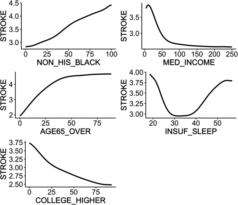
The partial dependence plot showing the marginal effect of each of five determinants on the neighborhood-level prevalence of stroke. Nonlinear patterns are observed for median household income, the proportion of people who are above 65, and the proportion of people with insufficient sleep

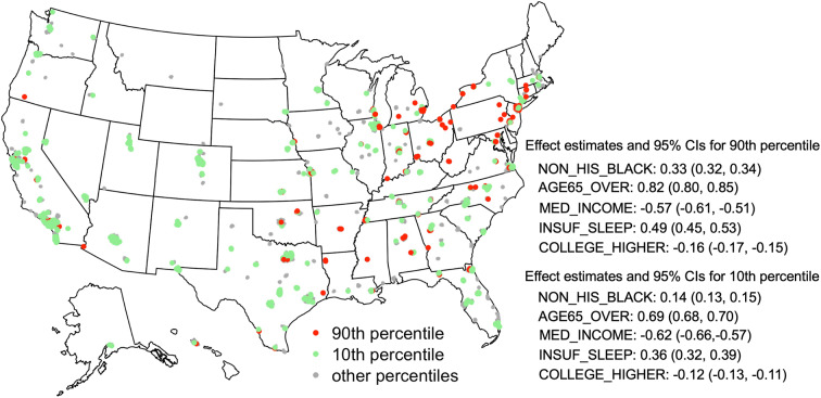
An “unblackboxing” analysis provided interpretable effects of the identified major determinants on the high prevalence of stroke at the neighborhood level. To demonstrate that a risk factor may have different effects on the tails of the outcome distribution than on the outcome on average, we examined the respective effects on the 90th (upper tail), 50th (median), and 10th (lower tail) quantile and the mean effects. Figure 7 displays the point estimates and 95% confidence intervals for each of the five major factor. First, larger shares of non-Hispanic blacks, older residents over 65 years of age, and people who have insufficient sleep were positively associated with higher 90th, median, and 10th quantile of the neighborhood-level prevalence of stroke. Median household income and the fraction of adults with higher education were inversely associated with all three quantiles. Second, all five major factors disproportionally affect different parts of the outcome distribution. The fractions of non-Hispanic blacks, older adults, highly educated residents, and people with insufficient sleep had significantly larger (absolute) effects on the upper tail than on the lower tail. Third, estimates from the mean-based LR analysis hardly covered the QR estimates. These findings suggest that analyses based on the premise that the prevalence of stroke is uniformly or symmetrically distributed across the nation would lead to an incomplete and biased summary of the effect of exposures. A geographical comparison of the effects on the 90th and 10th percentile appears in Fig. 8. Take the New York City as an example, Manhattan and Bronx sit at the opposite tails of stroke prevalence distribution (lower (10th percentile) and upper (90th percentile), respectively), the effects of major factors such as the prevalence of insufficient sleep and the age structure are substantially different (e.g., nonoverlapping confidence intervals of the effect estimates) between these two neighborhoods, underscoring heightened influence of insufficient sleep and older population in Bronx than in Manhattan, which, in turn, can provide guidance for developing targeted intervention programs.

Fig. 7.

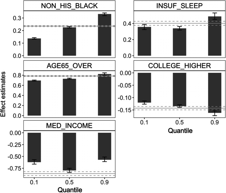
The effects of five major determinants on stroke varied across the 90th, 50th, and 10th quantile of the distribution of the neighborhood-level prevalence of stroke, in contrast to the uniform effect from the mean-based LR analysis. The height of the bars corresponds to estimated point effects; error bars represent the associated 95% confidence intervals. Horizontal gray solid and dotted lines represent the effects and confidence intervals on the mean responses. Effect estimates represent changes in the τth quantile (bars) or the mean (horizontal gray lines) of the prevalence of stroke per 10% increase in NON_HIS_BLACK, AGE65_OVER, INSUF_SLEEP, and COLLEGE_HIGHER and per $100,000 increase in MED_INCOME. LR linear regression

Fig. 8.

Effect estimates of five major neighborhood characteristics on the 90th and 10th quantile of the distribution of the neighborhood-level prevalence of stroke. Tracts corresponding to the 90th and 10th percentiles are represented by red and green dots, respectively

Discussion

In this study, we developed and applied a robust and reproducible machine learning–based approach to identify major factors for the tails of the distribution of the neighborhood-level cardiovascular health outcome, prevalence of stroke, and when the distribution was not normal and investigated the underlying effect mechanisms of the major factors, leveraging a high-performance nonparametric quantile regression technique, QRFs. We exploited a large-scale dataset with wide-ranging information from unhealthy behaviors and prevention measures to sociodemographic status and environmental factors, pooled from more than 20,000 census tracts in 500 cities of the USA.

Our approach identified a parsimonious set of predictors for quantiles of the neighborhood-level prevalence of stroke, shedding light on the true drivers for high prevalence of stroke at the neighborhood-level. The identified neighborhood characteristics were in good agreement with known individual-level risk factors. Neighborhoods with a larger share of non-Hispanic blacks, older adults, or people who have insufficient sleep tended to have a higher prevalence of stroke, whereas neighborhoods with a higher socio-economic status in terms of income and education had a lower prevalence of stroke. All of five factors disproportionally affected the prevalence of stroke among neighborhoods with different stroke prevalence profile. The effects on the 90th percentile (upper tail) were significantly higher than effects on the 10th percentile (lower tail) and higher than effects at the mean level. Using mean-based LR methods would have led to a limited and biased conclusion. Our approach offered a “higher-resolution” analysis that can be used to expand and deepen the existing quantitative evidence on stroke prevalence and its risk factors.

Results from our study may help inform public health policies. Establishing key neighborhood characteristics for high neighborhood-level prevalence of stroke allows policymakers to prioritize communities burdened with a high prevalence of stroke in developing and customizing community-based intervention programs to improve cardiovascular health outcomes. For example, resources may be allocated to the boroughs of New York City that have a high prevalence of stroke (e.g., the Bronx) to develop community-level educational interventions that promote exercise, improve bedroom ambience, or alleviate sleep disorders that may promote or interfere with sleep [31]. As the share of non-Hispanic blacks and the older population structure are two key components that may drive up the prevalence of stroke, it is critical for communities to make efforts to address avoidable inequalities and to eliminate health and health care disparities [32].

Identifying the most influential and true determinants from wide-ranging information is challenging, especially when the number of relevant predictors is sparse relative to the total number of available predictors and relationships between predictors and outcomes may be nonlinear. The presence of skewness in the outcome elevates the complexity. Previous studies that evaluated the relationships between neighborhood characteristics and cardiovascular health outcomes are typically conducted at the individual level and have limitations in analytical approaches [33]. The skewness of the outcome is typically ignored as mean-based regression analyses are commonly used. Predictors are often selected a priori or using test procedures based on some arbitrary threshold value. As a result, these studies may not provide specific insights into precise drivers for diverse neighborhoods with varied prevalence of cardiovascular diseases.

Our method is capable of specifying the effect of a predictor on the tail of the outcome distribution in the presence of skewedness that is missed by others. We compared our approach to classical QR and classical LR. Our approach achieved nearly the same prediction error reduction with only five predictors as the full QR model. In comparison, implementation of the two-standard-deviation approach within the framework of QRFs proposed in Fang et al. [28] selected only one variable, failing to capture many important predictors. Our “higher resolution” analysis showed that the major determinants disproportionally affected neighborhood-level stroke outcomes, underscoring the larger effects in the areas with a higher prevalence. In conjunction with the ranking of variable importance, our method can provide valuable guidance for targeted community-based interventions.

There are several limitations in this study. First, some behavioral and health outcome measures available in the 500 Cities Data were estimated by the CDC using a small area estimation approach. Although these estimated measures may not be accurate as real statistics, they provide the best available data for these small areas and the approach has been well validated [34]. Second, we could not make causal claims about the relationship between neighborhood characteristics and health outcomes due to the nature of the cross-sectional data and the ecological study design. However, our results identified important factors of neighborhood cardiovascular health and can potentially stimulate future causal inference research in neighborhood cardiovascular health. Finally, there could be other important variables that were not included in our study, either unmeasured or not collected in our data, due to the complexity of the neighborhood cardiovascular health. Despite the potential omitted variables, by combining data from three different large datasets and using an innovative machine learning approach, we believe that the scope and depth of our analysis can provide important insights on policymaking and lead to more innovative investigations in the area of neighborhood population health.

Conclusions

Highly flexible machine learning identifies drivers of neighborhood cardiovascular health outcomes from wide-ranging information in an agnostic and reproducible way. Quantile regression–based approaches provide an opportunity to deepen and expand the quantitative evidence gained from mean-based analyses. The identified major determinants and the effect mechanisms can provide important avenues for prioritizing and allocating resources to develop optimal community-level interventions for stroke prevention.

Funding

This research was supported in part by award ME2017C3 9041 from the Patient-Centered Outcomes Research Institute (PCORI), a grant from the National Heart, Lung, And Blood Institute of the NIH under Award Number R01HL141427, and two grants from the National Cancer Institute of the NIH under Award Number R21CA235153 and R21CA245855. The contents of this paper are solely the responsibility of the authors and do not necessarily represent the official views of the PCORI or NIH.

References

- 1.Mozaffarian D, Benjamin Emelia J, Go Alan S, et al. Heart disease and stroke statistics-2016 update. Circulation. 2016;133(4):e38–e360. doi: 10.1161/CIR.0000000000000350. [DOI] [PubMed] [Google Scholar]
- 2.You Roger X, McNeil John J, O’Malley Heather M, Davis Stephen M, Thrift Amanda G, Donnan GA. Risk factors for stroke due to cerebral infarction in young adults. Stroke. 1997;28(10):1913–1918. doi: 10.1161/01.STR.28.10.1913. [DOI] [PubMed] [Google Scholar]
- 3.Whisnant JP. Modeling of risk factors for ischemic stroke. Stroke. 1997;28(9):1840–1844. doi: 10.1161/01.STR.28.9.1840. [DOI] [PubMed] [Google Scholar]
- 4.Müller-Nordhorn J, Nolte Christian H, Rossnagel K, et al. Knowledge about risk factors for stroke. Stroke. 2006;37(4):946–950. doi: 10.1161/01.STR.0000209332.96513.82. [DOI] [PubMed] [Google Scholar]
- 5.Go AS, Mozaffarian D, Roger VL, Benjamin EJ, Berry JD, Blaha MJ, Dai S, Ford ES, Fox CS, Franco S, Fullerton HJ, Gillespie C, Hailpern SM, Heit JA, Howard VJ, Huffman MD, Judd SE, Kissela BM, Kittner SJ, Lackland DT, Lichtman JH, Lisabeth LD, Mackey RH, Magid DJ, Marcus GM, Marelli A, Matchar DB, McGuire D, Mohler ER, 3rd, Moy CS, Mussolino ME, Neumar RW, Nichol G, Pandey DK, Paynter NP, Reeves MJ, Sorlie PD, Stein J, Towfighi A, Turan TN, Virani SS, Wong ND, Woo D, Turner MB, American Heart Association Statistics Committee and Stroke Statistics Subcommittee Heart disease and stroke statistics-2014 update: a report from the American Heart Association. Circulation. 2014;129(3):e28–e292. doi: 10.1161/01.cir.0000441139.02102.80. [DOI] [PMC free article] [PubMed] [Google Scholar]
- 6.Bridgwood B, Lager KE, Mistri AK, Khunti K, Wilson AD, Modi P. Interventions for improving modifiable risk factor control in the secondary prevention of stroke. Cochrane Database Syst Rev. 2018;5(5):CD009103. doi: 10.1002/14651858.CD009103.pub3. [DOI] [PMC free article] [PubMed] [Google Scholar]
- 7.Cappuccio FP, Cooper D, D'Elia L, Strazzullo P, Miller MA. Sleep duration predicts cardiovascular outcomes: a systematic review and meta-analysis of prospective studies. Eur Heart J. 2011;32(12):1484–1492. doi: 10.1093/eurheartj/ehr007. [DOI] [PubMed] [Google Scholar]
- 8.Boehme AK, Esenwa C, Elkind MSV. Stroke risk factors, genetics, and prevention. Circ Res. 2017;120(3):472–495. doi: 10.1161/CIRCRESAHA.116.308398. [DOI] [PMC free article] [PubMed] [Google Scholar]
- 9.Kelly-Hayes M. Influence of age and health behaviors on stroke risk: lessons from longitudinal studies. J Am Geriatr Soc. 2010;58(Suppl 2):S325–S328. doi: 10.1111/j.1532-5415.2010.02915.x. [DOI] [PMC free article] [PubMed] [Google Scholar]
- 10.Schüle SA, Bolte G. Interactive and independent associations between the socioeconomic and objective built environment on the neighbourhood level and individual health: a systematic review of multilevel studies. PLoS One. 2015;10(4):e0123456. doi: 10.1371/journal.pone.0123456. [DOI] [PMC free article] [PubMed] [Google Scholar]
- 11.Osypuk TL, Ehntholt A, Moon JR, Gilsanz P, Glymour MM. Neighborhood differences in post-stroke mortality. Circ Cardiovasc Qual Outcomes. 2017;10(2):e002547. doi: 10.1161/CIRCOUTCOMES.116.002547. [DOI] [PMC free article] [PubMed] [Google Scholar]
- 12.Dworkis DA, Marvel J, Sanossian N, Arora S. Neighborhood-level stroke hot spots within major United States cities. Am J Emerg Med. 2020;38(4):794–98. 10.1016/j.ajem.2019.06.044. [DOI] [PubMed]
- 13.Karp David N, Wolff Catherine S, Wiebe Douglas J, Branas Charles C, Carr Brendan G, Mullen MT. Reassessing the Stroke Belt. Stroke. 2016;47(7):1939–1942. doi: 10.1161/STROKEAHA.116.012997. [DOI] [PMC free article] [PubMed] [Google Scholar]
- 14.Mensah GA, Cooper RS, Siega-Riz AM, Cooper LA, Smith JD, Brown CH, Westfall JM, Ofili EO, Price LSN, Arteaga S, Green Parker MC, Nelson CR, Newsome BJ, Redmond N, Roper RA, Beech BM, Brooks JL, Furr-Holden D, Gebreab SY, Giles WH, James RS, Lewis TT, Mokdad AH, Moore KD, Ravenell JE, Richmond A, Schoenberg NE, Sims M, Singh GK, Sumner AE, Treviño RP, Watson KS, Avilés-Santa ML, Reis JP, Pratt CA, Engelgau MM, Goff DC, Jr, Pérez-Stable EJ. Reducing cardiovascular disparities through community-engaged implementation research: a National Heart, Lung, and Blood Institute workshop report. Circ Res. 2018;122(2):213–230. doi: 10.1161/CIRCRESAHA.117.312243. [DOI] [PMC free article] [PubMed] [Google Scholar]
- 15.Wei Y, Kehm RD, Goldberg M, Terry MB. Applications for quantile regression in epidemiology. Curr Epidemiol Rep. 2019;6(2):191–199. doi: 10.1007/s40471-019-00204-6. [DOI] [Google Scholar]
- 16.Hu L, Hogan JW. Causal comparative effectiveness analysis of dynamic continuous-time treatment initiation rules with sparsely measured outcomes and death. Biometrics. 2019;75(2):695–707. doi: 10.1111/biom.13018. [DOI] [PMC free article] [PubMed] [Google Scholar]
- 17.500 Cities: Local Data for Better Health. Centers for Disease Control and Prevention; 2017. https://www.cdc.gov/500cities/index.htm. Accessed June 15, 2020.
- 18.American Community Survey 5-Year Data (2009-2018). United States Census Bureau. https://www.census.gov/data/developers/data-sets/acs-5year.html. Accessed June 15, 2020.
- 19.American FactFinder (AFF). United States Census Bureau. https://data.census.gov/cedsci/. Accessed June 15, 2020.
- 20.Environmental Justice Mapping and Screening Tool. United States Environmental Protection Agency. https://www.epa.gov/ejscreen. Accessed June.15, 2020.
- 21.Kuhn M, Johnson K. Applied predictive modeling. 2. New York: Springer; 2018. [Google Scholar]
- 22.Breiman L. Random forests. Mach Learn. 2001;45(1):5–32. doi: 10.1023/A:1010933404324. [DOI] [Google Scholar]
- 23.Genuer R, Poggi J-M, Tuleau-Malot C. Variable selection using random forests. Pattern Recogn Lett. 2010;31(14):2225–2236. doi: 10.1016/j.patrec.2010.03.014. [DOI] [Google Scholar]
- 24.Mazumdar M, Lin J-YJ, Zhang W, Li L, Liu M, Dharmarajan K, Sanderson M, Isola L, Hu L. Comparison of statistical and machine learning models for healthcare cost data: a simulation study motivated by Oncology Care Model (OCM) data. BMC Health Serv Res. 2020;20(1):350. doi: 10.1186/s12913-020-05148-y. [DOI] [PMC free article] [PubMed] [Google Scholar]
- 25.Meinshausen N. Quantile regression forests. J Mach Learn Res. 2006;7:983–999. [Google Scholar]
- 26.Dietrich S, Floegel A, Troll M, Kühn T, Rathmann W, Peters A, Sookthai D, von Bergen M, Kaaks R, Adamski J, Prehn C, Boeing H, Schulze MB, Illig T, Pischon T, Knüppel S, Wang-Sattler R, Drogan D. Random Survival Forest in practice: a method for modelling complex metabolomics data in time to event analysis. Int J Epidemiol. 2016;45(5):1406–1420. doi: 10.1093/ije/dyw145. [DOI] [PubMed] [Google Scholar]
- 27.Wang L, Wu Y, Li R. Quantile regression for analyzing heterogeneity in ultra-high dimension. J Am Stat Assoc. 2012;107(497):214–222. doi: 10.1080/01621459.2012.656014. [DOI] [PMC free article] [PubMed] [Google Scholar]
- 28.Fang Y, Xu P, Yang J, Qin Y. A quantile regression forest based method to predict drug response and assess prediction reliability. PLoS One. 2018;13(10):e0205155. doi: 10.1371/journal.pone.0205155. [DOI] [PMC free article] [PubMed] [Google Scholar]
- 29.Darst BF, Malecki KC, Engelman CD. Using recursive feature elimination in random forest to account for correlated variables in high dimensional data. BMC Genet. 2018;19(1):65. doi: 10.1186/s12863-018-0633-8. [DOI] [PMC free article] [PubMed] [Google Scholar]
- 30.Ishwaran H, Kogalur UB, Chen X, Minn AJ. Random survival forests for high-dimensional data. Stat Anal Data Min ASA Data Sci J. 2011;4(1):115–132. doi: 10.1002/sam.10103. [DOI] [Google Scholar]
- 31.Redeker NS, Caruso CC, Hashmi SD, Mullington JM, Grandner M, Morgenthaler TI. Workplace interventions to promote sleep health and an alert, Healthy Workforce. J Clin Sleep Med. 2019;15(4):649–657. doi: 10.5664/jcsm.7734. [DOI] [PMC free article] [PubMed] [Google Scholar]
- 32.Srinivasan S, Williams SD. Transitioning from health disparities to a health equity research agenda: the time is now. Public Health Rep. 2014;129(Suppl 2):71–76. doi: 10.1177/00333549141291S213. [DOI] [PMC free article] [PubMed] [Google Scholar]
- 33.Kershaw KN, Osypuk TL, Do DP, De Chavez PJ, Diez Roux AV. Neighborhood-level racial/ethnic residential segregation and incident cardiovascular disease: the multi-ethnic study of atherosclerosis. Circulation. 2015;131(2):141–148. doi: 10.1161/CIRCULATIONAHA.114.011345. [DOI] [PMC free article] [PubMed] [Google Scholar]
- 34.Zhang X, Holt JB, Yun S, Lu H, Greenlund KJ, Croft JB. Validation of multilevel regression and poststratification methodology for small area estimation of health indicators from the behavioral risk factor surveillance system. Am J Epidemiol. 2015;182(2):127–137. doi: 10.1093/aje/kwv002. [DOI] [PMC free article] [PubMed] [Google Scholar]