

Summary:
Primates recognize complex objects such as faces with remarkable speed and reliability. Here, we reveal the brain’s code for facial identity. Experiments in macaques demonstrate an extraordinarily simple transformation between faces and responses of cells in face patches. By formatting faces as points in a high-dimensional linear space, we discovered that each face cell’s firing rate is proportional to the projection of an incoming face stimulus onto a single axis in this space, allowing a face cell ensemble to encode the location of any face in the space. Using this code, we could precisely decode faces from neural population responses and predict neural firing rates to faces. Furthermore, this code disavows the longstanding assumption that face cells encode specific facial identities, confirmed by engineering faces with drastically different appearance that elicited identical responses in single face cells. Our work suggests other objects could be encoded by analogous metric coordinate systems.
Graphical Abstract
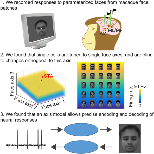
Facial identity is encoded via a remarkably simple neural code that relies on the ability of neurons to respond to facial features along specific axis in the space, disavowing the longstanding assumption that single face cells encode individual faces.
Introduction:
A central challenge of visual neuroscience is to understand how the brain represents the identity of a complex object. This process is thought to happen in IT cortex, where neurons carry information about high-level object identity, with invariance to various transformations that do not affect identity (Brincat and Connor, 2004; Ito et al., 1995; Majaj et al., 2015). However, despite decades of research on the response properties of IT neurons, the precise code for object identity used by single IT neurons remains unknown: typically, neurons respond to a broad range of stimuli and the principles governing the set of effective stimuli are not understood. Ideally, if we had a full understanding of IT cortex, then we would be able to decode the precise object presented from IT population responses, and conversely predict IT responses to an arbitrary object. Due to the many layers of computation between the retina and IT cortex, it has been suggested that a simple, explicit model of IT cells may be impossible to achieve (Yamins et al., 2014).
Here, we sought to construct an explicit model of face-selective cells that would allow us to both decode an arbitrary realistic face from face cell responses, and predict the firing of cells in response to an arbitrary realistic face. Studying face coding has two unique advantages. First, the macaque face patch system, a set of regions strongly selective for faces in fMRI experiments, provides a powerful experimental model to dissect the mechanism for face representation, since these regions contain high concentrations of face-selective cells (Tsao et al., 2006) and appear to perform distinct steps in face representation (Freiwald and Tsao, 2010). Second, the homogeneity of faces as a stimulus class permits arbitrary faces to be represented by relatively small sets of numbers describing coordinates within a “face space” (Beymer and Poggio, 1996; Blanz and Vetter, 1999; Edwards et al., 1998), facilitating systematic exploration of the full geometry of neuronal tuning.
To explore the geometry of tuning of high-level sensory neurons in a high-dimensional space, we recorded responses of cells in face patches ML/MF and AM to a large set of realistic faces parameterized by 50 dimensions. We chose to record in ML/MF and AM because previous functional (Freiwald and Tsao, 2010) and anatomical (Grimaldi et al., 2016; Moeller et al., 2008a) experiments have demonstrated a hierarchical relationship between ML/MF and AM, and suggest that AM is the final output stage of IT face processing. In particular, a population of sparse cells has been found in AM which appear to encode exemplars for specific individuals, as they respond to faces of only a few specific individuals, regardless of head orientation (Freiwald and Tsao, 2010). These cells encode the most explicit concept of facial identity across the entire face patch system, and understanding them seems crucial for gaining a full understanding of the neural code for faces in IT cortex.
Our data reveal a remarkably simple code for facial identity in face patches ML/MF and AM that can be used to both precisely decode realistic face images from population responses and accurately predict neural firing rates. Single cells in both ML/MF and AM are essentially projecting incoming faces, represented as vectors in face space, onto specific axes. A prediction of this model is that each cell should have a linear null space, orthogonal to the preferred axis, in which all faces elicit the same response. We confirm this prediction, even for sparse AM cells which had previously been assumed to explicitly code exemplars of specific identities.
Results:
Recording procedure and stimulus generation
We first localized six face patches in two monkeys with fMRI by presenting a face localizer stimulus set containing images of faces and non-face objects (Moeller et al., 2008b; Tsao et al., 2003; Tsao et al., 2008). Middle face patches MF, ML, and anterior patch AM were targeted for electrophysiological recordings (Tsao et al., 2006) (Figure S1A). Well-isolated single units were recorded while presenting 16 real faces and 80 non-face objects (same stimuli as in (Tsao et al., 2006)). Units selective for faces were selected for further recordings (Figures S1B and C, see STAR Methods).
To investigate face representation in face patches, we generated parameterized realistic face stimuli using the “active appearance model” (Cootes et al., 2001; Edwards et al., 1998): for each of 200 frontal faces from an online face database (FEI face database; see STAR Methods: Generation of parameterized face stimuli), a set of landmarks were labeled by hand (Figure 1A, left). The positions of these points carry information about the shape of the face and the shape/position of internal features (Figure 1A, middle). Then the landmarks were smoothly morphed to a standard template (average shape of landmarks); the resulting image (Figure 1A, right) carries shape-free appearance information. In this way, we extracted a set of 200 shape descriptors and 200 appearance descriptors. To construct a realistic face space, we performed principal components analysis on the shape and appearance descriptors separately, to extract the feature dimensions that accounted for the largest variability in the database, retaining the first 25 PCs for shape and first 25 PCs for appearance (Figure 1B, Figure S2A). This results in a 50-d face space, where every point represents a face, obtained by starting with the average face, first adding the appearance transform, and then applying the shape transform to the landmarks; reconstructions of faces from the original data set within this 50-d space strongly resemble the original faces (Figure S2B). Most of the dimensions were “holistic”, involving changes in multiple parts of the face; for example, the first shape dimension involved changes in hairline, face width, and height of eyes. Movie S1 shows a movie of a face undergoing only changes in shape parameters, and a face undergoing changes only in appearance parameters.
Figure 1. Complementary representation of facial features by AM and ML/MF populations.
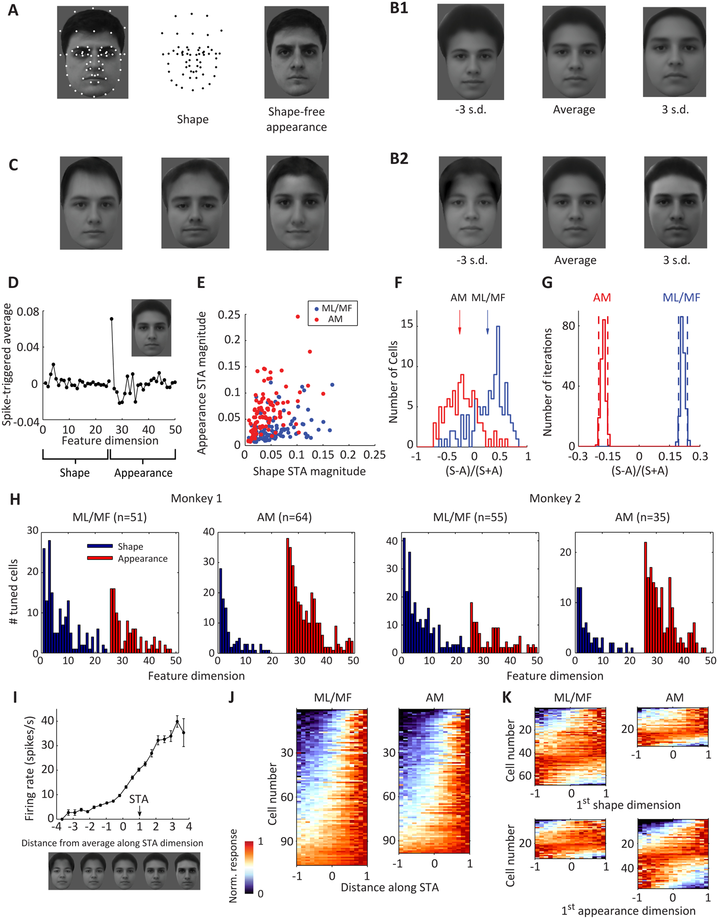
A-C, Generation of parameterized face stimuli. A, 58 landmark points were labeled on 200 facial images from a face database (FEI face database; example image shown on left). The positions of these landmarks carry shape information about each facial image (middle). The landmarks were smoothly morphed to match the average landmark positions in the 200 faces, generating an image carrying shape-free appearance information about each face (right). B, Principal component analysis was performed to extract the feature dimensions that account for the largest variability in the database. The 1st principal component for shape (B1) and appearance (B2) are shown. C, Example face stimuli generated by randomly drawing from a face space constructed by the first 25 shape PCs and first 25 appearance PCs. D, Spike-triggered average of a face-selective neuron from anterior face patch AM. The first 25 points represent shape dimensions, and the next 25 represent appearance dimensions. The facial image corresponding to the STA is shown in the inset. E, Vector length of the STA for the 25 appearance dimensions is plotted against that for the 25 shape dimensions for all the cells recorded from middle face patches ML/MF (blue) and anterior face patch AM (red). F, Distribution of shape preference indices, quantified as the contrast between the vector length of shape and appearance STA for ML/MF and AM cells. Arrows indicate the average of each population (p=10−25, Student’s t-test). G, Reliability of the estimated population average of shape preference index for ML/MF and AM (n = 200 iterations of random sampling with replacement). Dash lines indicate 95% confidence intervals. H, Number of significantly tuned cells (p<0.01 by shift predictor, see STAR Methods) for each of 50 dimensions for ML/MF and AM cells in both monkeys. I, Response of a neuron in AM is plotted against distance between the stimulus and the average face along the STA axis. Error bars represent s.e. J, Responses of ML/MF (left) and AM (right) neurons as a function of the distance along STA dimension. The abscissa is rescaled so that the range [−1,1] covers 98% of the stimuli. K, Neuronal responses as a function of the feature value for the 1st shape dimension (top) and 1st appearance dimension (bottom) for all significant cells (p<0.01 by shift predictor).
To generate stimuli for our recordings, we randomly drew 2000 faces from this face space (Figure 1C). Projections of real faces onto the 50 axes were largely Gaussian, and the 2000 faces shared a similar distribution of vector lengths as the real faces (Figure S2C). Face stimuli were presented for 150 ms (ON period) interleaved by a gray screen for 150 ms (OFF period), and the same set of 2000 stimuli were presented to each cell from three to five times each. We recorded 205 cells in total from two monkeys: 51 cells from ML/MF and 64 cells from AM for monkey 1; 55 cells from ML/MF and 35 cells from AM for monkey 2.
Face patches ML/MF and AM carry complementary information about facial features
To quantify neuronal tuning to the 50 dimensions of the face space, responses of each neuron were first used to calculate a “spike-triggered average” (STA) stimulus (Schwartz et al., 2006), i.e., the average stimulus that triggered the neuron to fire (Figure 1D). On average, each cell was significantly tuned along 6.1 feature dimensions (covering the range [0 17] with s.d.=3.8). We next compared the relative sensitivity to shape or appearance for each neuron: a “shape preference index” was computed based on the vector length of the STA for shape vs. appearance dimensions. We found that most ML/MF cells showed stronger tuning to shape dimensions than to appearance dimensions, while AM cells showed the opposite trend (Figure 1E–H). The shape preference indices computed with subsets of stimuli were highly correlated (split halves approach, correlation=0.89±0.07, n=205 cells, see STAR Methods), hence this distinction between preferred axes in ML/MF and AM is real (Figure 1G). Furthermore, this distinction is completely consistent with previous studies showing that ML/MF cells are tuned to specific face views, while AM cells code view-invariant identity (Freiwald and Tsao, 2010). Changes in identity would produce changes in appearance dimensions, and changes in view (within a limited range away from frontal) would be accounted for by changes in shape dimensions. Importantly, because shape dimensions encompass a much larger set of transformations than just view changes, the tuning of AM cells to appearance dimensions indicates invariance to a much larger set of transformations in articulated shape than just view changes, consistent with the invariance of face recognition behavior to many transformations beyond view changes, such as severe distortion in face aspect ratio (Sinha et al., 2006).
Next we explored the shape of tuning to shape/appearance dimensions by ML/MF and AM neurons. When responses of an example AM neuron were grouped according to the distance between the stimulus and the average face (i.e., the face at the origin of the face space) along the STA axis in the 50-d face space, we saw ramp-like tuning, with maximum and minimum responses occurring at extreme feature values (Figure 1I). Such ramp-like tuning was consistently observed along the STA dimension across the population for both AM and ML/MF (Figure 1J), and was also clear for individual dimensions (Figure 1K).
Decoding facial features using linear regression
If a face cell has ramp-shaped tuning to different features, this means that its response can be roughly approximated by a linear combination of the facial features, with the weighting coefficients given by the slopes of the ramp-shaped tuning functions. For a population of neurons, , where is the vector of responses of different neurons, S is the matrix of weighting coefficients for different neurons, is the 50-d vector of face feature values, and is the offset vector. If this is true, then by simply inverting this equation, we should be able to linearly decode the facial features from the population response (Cowen et al., 2014; Kay et al., 2008; Nestor et al., 2016). To attempt this, we took advantage of the fact that we always presented the same set of 2000 stimuli to the monkey, and used a leave-one-out approach to train and test our model. We determined the transformation from responses to feature values with linear regression using population responses of face cells in a time window from 50 to 300 ms after stimulus onset to 1999 faces, and then predicted the feature value of the remaining image (Figure 2A). Note that for this decoding procedure, we used cells recorded sequentially; if the brain were to use a similar decoding approach, it would be using neurons firing simultaneously.
Figure 2. Decoding facial features using linear regression.
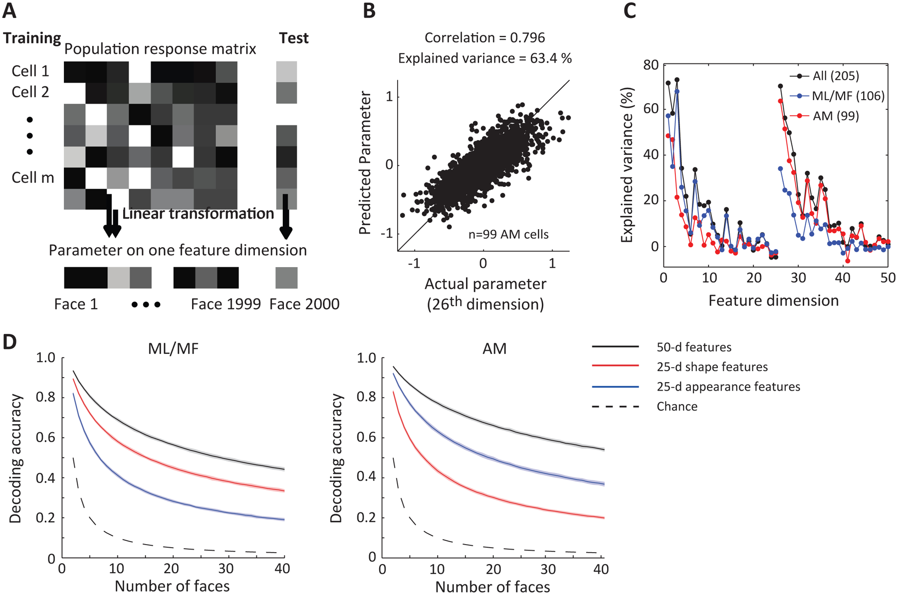
A, Diagram illustrating decoding model. To construct and test the model, we used responses of AM (n=99) and ML/MF (n=106) cells to 2000 faces. Population responses to 1999 faces were used to determine the transformation from responses to feature values by linear regression, and then the feature values of the remaining image were predicted. B, Model predictions using AM data are plotted against actual feature values for the first appearance dimension (26th dimension). C, Percentage explained variances for all 50 dimensions using linear regression based on responses of three different neuronal populations: 106 ML/MF cells (blue); 99 AM cells (red); 205 cells combined (black). D, Decoding accuracy as a function of the number of faces randomly drawn from the stimulus set for three different models (see STAR Methods). For each model, different sets of features were first linearly decoded from population responses, and then Euclidean distances between decoded and actual features in each feature space were computed to determine decoding accuracy. The three sets of features are: 50-d features of active appearance model; 25-d shape features; 25-d appearance features. Shaded region indicates s.d. estimated using bootstrapping.
We found this simple linear model could predict single features very well (Figure 2B). We used percentage variance of the feature values explained by the linear model to quantify the decoding quality. Overall, the decoding quality for appearance features was better than that for shape features for AM neurons while the opposite was true for ML/MF neurons (Figure 2C and D), consistent with our analysis using STA (Figure 1F). By combining the predicted feature values across all 50 dimensions, we could reconstruct the face that the monkey saw. Examples of the reconstructed faces are shown in Figure 3A next to the actual faces, using ML/MF data, AM data, and combined data from both patches. The reconstructions using AM data strongly resemble the actual faces the monkey saw, and the resemblance was further improved by adding ML/MF data.
Figure 3. Reconstruction of facial images using linear regression.
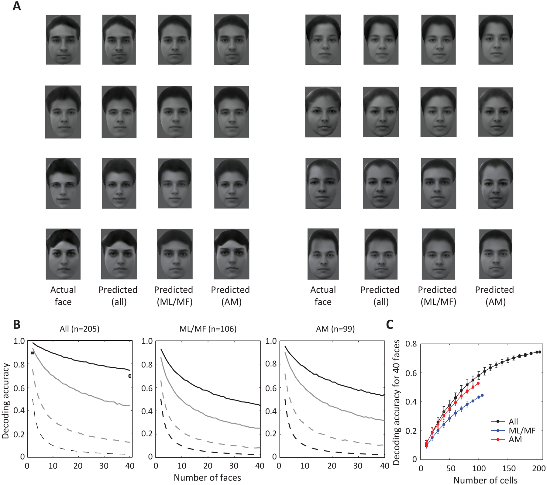
A, Using facial features decoded by linear regression in Figure 2, facial images could be reconstructed. Predicted faces by three neuronal populations and the corresponding actual stimuli presented in the experiment are shown. B, Decoding accuracy as function of number of faces, using a Euclidean distance model (black solid line). Decoding accuracy based on two alternative models, nearest neighbor in the space of population response (gray dashed line, see STAR Methods) and average of nearest 50 neighbors (gray solid line), were much lower. The black dashed line represents chance level. Results based on three neuronal populations are shown separately (black solid lines for ML/MF and AM are the same as the black solid lines for corresponding patches in Figure 2D, except here they are not shown with variability estimated by bootstrapping). In the left panel, boxes and error bars represent mean and s.e.m. of subjective (human-based) decoding accuracy based on 78 human participants (see STAR Methods: human psychophysics). C, Decoding accuracy for 40 faces plotted against different numbers of cells randomly drawn from three populations (black: all; blue: ML/MF; red: AM). Error bar represents s.d.
To quantify the overall decoding accuracy of our model, we randomly selected a number of faces from the stimulus set and compared their actual 50-d feature vectors to the reconstructed feature vector of one face in the set using Euclidean distance. The decoding accuracy decayed with increasing number of faces, but was ~ 75% with 40 faces when all cells were pooled together (Figure 3B, black solid line), which is much higher than chance level (Figure 3B black dashed line). Furthermore, when the number of cells was equalized, decoding accuracy rose fastest for the combined population compared to ML/MF and AM populations alone (Figure 3C, for n=99 cells, p<0.01 when comparing combined population with AM; p<0.005 when comparing combined population with ML/MF, estimated by 1000 iterations of random sampling with replacement, see STAR Methods), consistent with the two regions carrying complementary information about shape and appearance. We also determined the accuracy of decoding by measuring the subjective similarity between the reconstructions and actual faces using human psychophysics, and found that human subjects were significantly more likely to match the reconstructed with the actual face, compared to a highly similar distractor (see STAR Methods: human psychophysics). The fact that we can accurately decode the identity of real faces from population responses in ML/MF and AM shows that we have satisfied one essential test of a full understanding of the brain’s code for face identity.
Shape of tuning along axes orthogonal to the STA
The model used for decoding assumes that face patch neurons are linearly combining different features (“axis model”). While simple, this code is inconsistent with prevailing notions of the function of IT cells, in particular sparse AM cells. Many models of object recognition assume an exemplar-based representation (Riesenhuber and Poggio, 1999; Valentine, 1991) (Figure 4G, right), in which object recognition is mediated by units tuned to exemplars of specific objects that need to be recognized. Early studies attempting to find the “optimal object” for IT cells assumed such an exemplar-based model (Tanaka, 1996). More direct support for an exemplar-based model comes from recordings in face patch AM, where a subset of cells have been found to respond extremely sparsely to only a few identities, invariant to head orientation (e.g., see Figure 1 in (Freiwald and Tsao, 2010) and Movie S2). These cells have been hypothesized to code exemplars of specific individuals, analogous to the “Jennifer Aniston” cells recorded in human hippocampus which respond to images, letter strings, and vocalizations of one specific individual (Quiroga et al., 2005). If AM cells are in fact linearly combining different features, then geometrically, what an AM cell is doing is simply taking a dot product between an incoming face and a specific direction in face space defined by the cell’s STA (Figure 4A, inset). If this is true, then each cell should have a null space within which the response of the cell doesn’t change. This null space is simply the plane orthogonal to the STA, since adding a vector in this plane won’t change the value of projection onto the STA. In contrast, if AM cells are coding exemplars of specific individuals, then the response to an incoming face should be a decreasing function of distance of the face to the exemplar face (Riesenhuber and Poggio, 1999; Valentine, 1991).
Figure 4. AM neurons display almost flat tuning along axes orthogonal to the STA in face space.
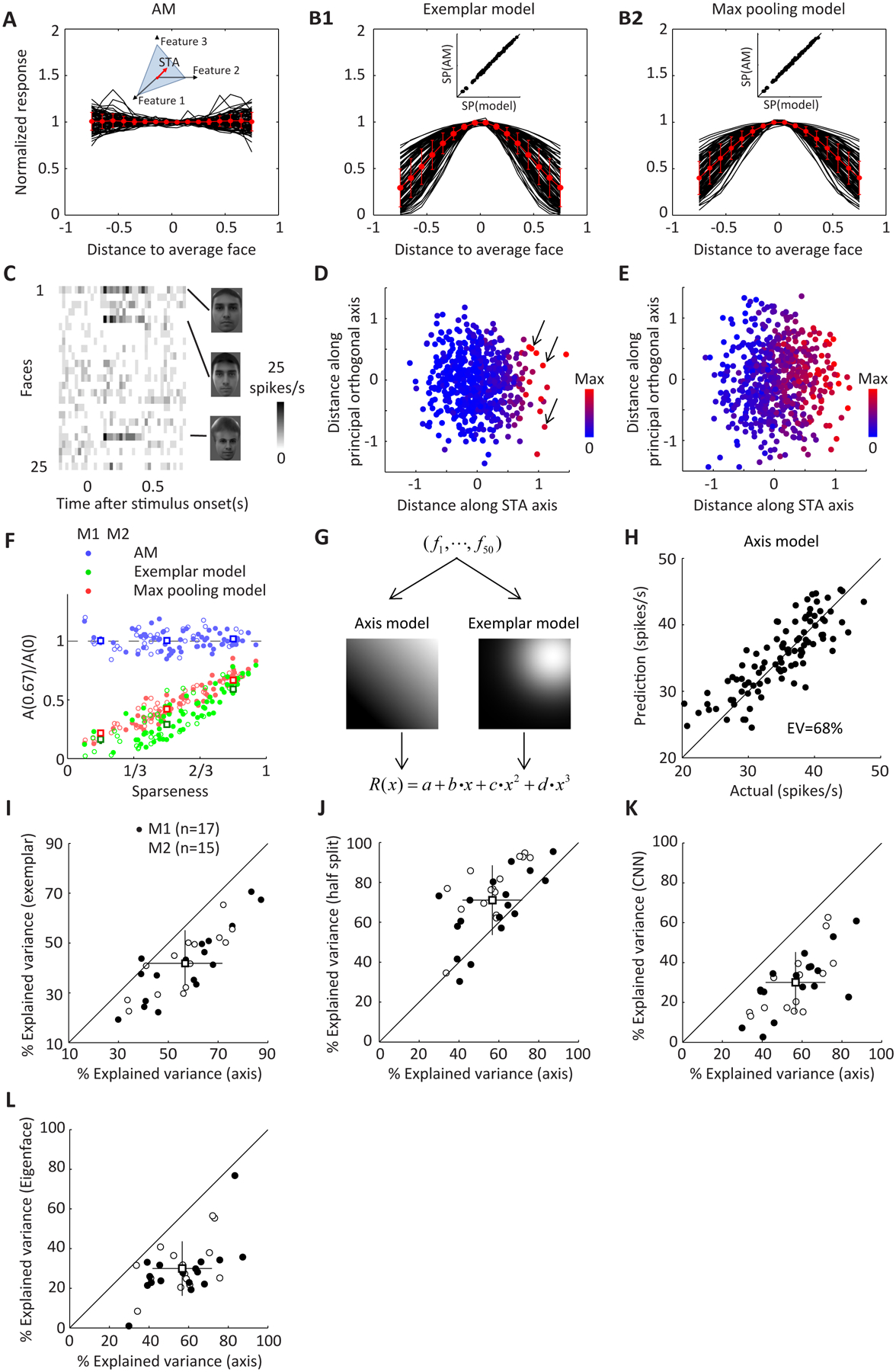
A, For each neuron in AM, the STA was first computed, then 2000 random axes were selected and orthogonalized to the STA in the 25-d space of appearance features. Tuning functions along 300 axes accounting for the largest variability in the stimuli were averaged and fitted with a Gaussian function (). The center of the fit (a + c) was used to normalize the average tuning function. Red dots and error bars represent mean and s.d. of the population. B, Same as A, but for two control models. B1, Each simulated cell corresponds to one of the 200 real faces projected onto the 25-d face space of appearance features (exemplar face), and its response to an arbitrary face is a decreasing linear function of the Euclidean distance between the arbitrary face and the exemplar in the 25-d feature space. B2, Each simulated cell corresponds to 81 transforms of a single identity (9 views*9 positions). For a given image, the similarity of this image to any of the transforms (defined as a decreasing linear function of pixel level distance between the two images) was computed and the maximum value across all 81 transforms was set as the response of the cell. For fairness of comparison, the response of each model cell was matched to one of the AM neurons on noise level and sparseness (for details see STAR Methods, comparison of sparseness between neurons and models is shown in the inset). C, Responses of an AM neuron to 25 parameterized faces. Firing rate was averaged with 25 ms bins. The three stimuli evoking strong responses are shown on the right. D, Responses of the cell in (C) to different faces are color coded and plotted in the 2-D space spanned by the STA axis and the axis orthogonal to STA in the appearance feature space accounting for the largest variability in the features. Arrows indicate three faces in (C). E, Same as D, but for a non-sparse AM cell. F, For each cell in AM or two models, tuning along orthogonal axes was first fitted with a Gaussian function, and the ratio between the fit at and the center (a + c) and was computed and plotted against the sparseness of the cell. Cells in each population were further divided into three groups according to sparseness . Solid and open circles indicate data from two different monkeys. Boxes and error bars represent mean and s.e. of each subgroup. The difference between AM neurons and two models was significant for all three sparseness levels (p<0.001, Student’s t-test). G, Two models were used to fit face cells’ responses to parameterized face stimuli: 1) an “axis” model where every face was projected onto an axis in the 50-d face space; 2) an “exemplar” model where distance from one of the 2000 faces to an exemplar face was computed (the length of the exemplar face in the 50-d space was restricted to be smaller than twice the average length of real faces). The projection or distance was then passed through a nonlinearity (a third-order polynomial) to generate a predicted response. Each parameter of the model was adjusted using gradient descent to minimize the Euclidean distance between predicted and actual firing rate. To obtain high-quality responses, we repeated 100 faces more frequently than the remaining 1900 faces, and used responses to the 100 faces to validate the model derived from the 1900 faces. H, Predicted versus actual responses for one example cell using an axis model. The model explained 68% of variance in the responses. I, Comparison of fitting quality by two models for 32 cells. An axis model provides significantly better fits to actual responses (mean=56.9%) than an exemplar model (mean=41.7%, p<0.001, paired t-test). J, Different trials of responses to 100 stimuli were randomly split into 2 halves, and the average response across half of the trials was used to predict that of the other half. Percentage variances explained, after Spearman-Brown correction (mean=71.1%), are plotted against that of the axis model. K, A convolutional neural net was trained to perform view-invariant face identification (Figure S7). 52 units were randomly selected from 500 units in the final layer of CNN and were used to linearly fit responses of face cells. Mean explained variance across 100 repetitions of random sampling was plotted against that of the axis model. The fit quality by CNN units was much lower (mean=30.2%, p<0.01) than the axis model. Using more units will lead to overfitting and the validated explained variance will be further reduced (to 26.5% for the case of 100 units and 17.7% for 200 units). L, Neuronal responses were fitted by a different “axis” model using “Eigenface” features as the dimensions of the face space (Figure S2G, see STAR Methods). PCA was performed on the original image intensities of 2000 faces and the first 50 PCs were treated as the input to the axis model. Fitting procedure was the same as shown in (G). The fit quality by “Eigenface” model was much lower (mean=29.9%, p<0.001) than the axis model. Using 100 PCs slightly increased the fit quality (mean=31.1%), while using 200 PCs led to overfitting (mean=22.8%).
To decide whether a cell is coding an exemplar or an axis, the critical question is: what is the shape of tuning along axes in the plane orthogonal to the STA axis? If this plane constitutes a “null space” in which all faces elicit the same response, this would be indicative of axis coding. Alternatively, if there is Gaussian tuning along axes within this plane, this would be indicative of exemplar coding. To distinguish between these two possibilities, we quantified tuning of AM cells along axes orthogonal to the STA in 25-d appearance feature space (Figure 4A); we purposely excluded the 25-d shape feature space to avoid the possibility of shape invariance giving rise to flat tuning along the orthogonal dimension. To obtain better signal quality, we averaged tuning along multiple axes that accounted for the largest variability of the stimuli (see STAR Methods; the results also hold true for single axes, see Figure S3). Surprisingly, the tuning of AM neurons was largely flat along orthogonal axes and showed no clear bias for Gaussian nonlinearity.
To quantitatively confirm the flatness, we compared the result with several models (Figure 4B, Figure S3B–D). The first model defined, for each AM cell recorded, a counterpart model “exemplar” cell which fired maximally to a specific exemplar face, and whose firing rate decayed linearly as a function of the distance between an incoming face and the exemplar face. We chose the exemplar face by projecting one of the 200 real faces in the original FEI database to the 25-d appearance feature space. The sparseness and noise of the model units were set equal to those of the actual units. As expected, the model units displayed clear bell-shaped tuning along orthogonal axes (Figure 4B1). In a second exemplar model, we implemented view-invariance by a conventional max-pooling operation: each unit contained a set of templates corresponding to different views and positions of the same identity, and the response of the unit to one face was the maximum of the similarities between this face and each template (similarity was defined as a decreasing linear function of mean absolute pixel difference between two images). This model also demonstrated a clear bell-shaped nonlinearity (Figure 4B2).
One might worry that the flat tuning we observed in the orthogonal plane was due to contribution from dimensions that did not modulate any cells in the population; analysis of responses restricted to the actual face space spanned by the STAs of AM neurons shows that this is not the case (Figure S4A–H). Another concern is that cells may encode exemplars using an ellipsoidal distance metric, such that tuning is broader along some dimensions than others; analysis of model exemplar units explicitly endowed with non-circular aspect ratio rule out this possibility (Figure S4I–L).
A further potential confounding factor is adaptation: cells in IT cortex have been reported to suppress their responses more strongly for more frequent feature values (Vogels, 2016). Our stimuli were Gaussian distributed along each axis; as a result faces closer to the average appeared more frequently. To rule out the possibility that our findings are specific to our stimulus conditions, we examined the extent of adaptation in the recorded cells by regrouping the responses based on the preceding stimuli. We first examined how tuning along the STA dimension is affected by the preceding stimuli. The responses of each cell were regrouped according to the distance between the immediately preceding stimulus and the average face along the STA dimension, into a far group (33% largest distances) and a near group (33% smallest distances). If adaptation plays an important role, one would expect to see a clear difference in tuning between the two groups (for example, one might expect the center of the tuning function to be more suppressed for the “near” group than the “far” group). However, we observed no difference in tuning between the two groups (Figures S5A–D). Similar to results along the STA dimension, we found adaptation played little role in reshaping tuning along orthogonal axes (Figures S5E–H).
The results so far suggest that AM cells are encoding specific axes rather than exemplars. How can we reconcile this finding with the existence of sparse, view-invariant AM cells selective for specific exemplars? To address this, we examined the shape of tuning of AM cells as a function of sparseness. We found that for our parameterized stimuli, some AM neurons also responded sparsely (Figure 4C shows one example). However, when we looked at tuning of these sparse neurons in a 2-d space spanned by the STA and an orthogonal axis, they showed a drastic nonlinearity along the STA, but nearly no tuning along the orthogonal axis (Figure 4D shows one example; for comparison, Figure 4E shows the response of a non-sparse cell). When we plotted the level of nonlinearity along the orthogonal axis against sparseness, we found AM neurons were less tuned than the two control models, regardless of the sparseness of responses (Figure 4F, Figures S3E–H). Furthermore, the lack of tuning along the orthogonal axis provides a simple explanation for the mystery of why some AM cells, even super sparse ones, respond to several faces bearing no obvious resemblance to each other: these faces are “metameric” because they differ by a large vector lying in the cell’s null space (arrows in Figure 4D).
We repeated the above analyses for cells in ML/MF, and found that ML/MF cells were also tuned to single axes defined by the STA, showing flat tuning in the hyperplane orthogonal to the STA (Figures S4M and N). Thus the fundamental difference between ML/MF and AM lies in the axes being encoded (shape versus shape-free appearance), not in the coding scheme.
A full model of face processing should allow both encoding and decoding of neural responses to arbitrary faces. How well does the axis model predict firing rates of cells to real faces? To address this, we fit responses of face cells to two models, an axis model and an exemplar model (Figure 4G). In the axis model, we assumed that the cell is simply taking the dot product between an incoming face (described in terms of a 50-d shape-appearance vector) and a specific axis, and then passing the result through a nonlinearity. In the exemplar model, we assumed the cell is computing the Euclidean distance between the face and a specific exemplar face and then passing the result through a nonlinearity. The nonlinearity allows us to account for nonlinear tuning along the STA. We fit the two models on responses to a set of 1900 faces, and then tested on responses to a different set of 100 faces. To obtain high signal quality, the 100 faces were repeated 10 times more frequently than the rest of the 1900 faces. We found that the axis model could explain up to 57% of the variance of the response, outperforming the exemplar model by more than 15% of explained variance (Figures 4H and I). We compared this to the noise ceiling of the cells estimated by using the mean response on half of the trials to predict the mean on the other half, which yielded 72% explained variance after Spearman-Brown correction (Figure 4J). The ratio between variances explained by the axis model and that by data is 80.0%, which is much higher than previously achieved (48.5%)(Yamins et al., 2014). We also trained a five-layer convolutional neural network (CNN) to perform invariant face identification, and then linearly regressed activity of AM cells on the activity of the output neurons of this network, analogous to a previous study using output units of a CNN trained on invariant object recognition to model IT responses (Yamins et al., 2014). We found this could explain 30% variance (42.5% of noise ceiling) (Figure 4K), significantly lower than the performance of the axis model, and comparable to results of the previous study (48.5% of noise ceiling). Furthermore, we compared the axis model with a well-known face model: the “Eigenface” model (Sirovich and Kirby, 1987; Turk and Pentland, 1991), which computes principal components of the original images rather than shape or appearance representations (STAR Methods, see also Figure S2G). In this case, 50 “Eigenface” features were used as the axes of the model. We found that the “Eigenface” model could explain 31% variance (Figure 4L), significantly lower than that of the axis model. This suggests the correct choice of face space axes is critical for achieving a simple explanation of face cells’ responses.
So far, all of our results point to a model of face cells as linear projection machines. While simple, this model is also surprising because it means face cells are performing a rather abstract mathematical computation. We next performed a strong test of this model: (1) we computed, online during the recording, the STA of a cell, (2) we used the STA to engineer a set of predicted face metamers for the cell (i.e., faces lying in the plane orthogonal to the STA), and (3) we measured responses of the cell to these face metamers. Specifically, we presented faces evenly sampled from a 2-d space spanned by the STA axis and the principal orthogonal axis (Figure 5A, STAR Methods) while recording from the same cell in which the STA was measured. We found that, as predicted, face cells showed strong tuning only along the STA axis, with nearly identical responses to faces varied along orthogonal axes (Figures 5B–E).
Figure 5. Responses of AM cells to faces specifically engineered for each cell confirms the axis model.
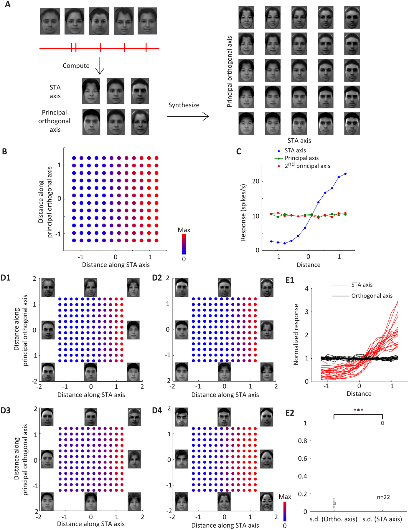
A, Experimental procedure. After recording the responses of a face cell to 2000 parameterized face stimuli, the STA axis and the principal orthogonal axis were extracted. Facial features were evenly sampled along each axis and a facial image was synthesized for each pair of features (see STAR Methods). The synthesized images were presented to the monkey and responses of the same face cell were recorded. B, The responses of an AM cell to 144 faces evenly sampled from the 2-d space spanned by the STA axis and principal orthogonal axis (c.f. Figure 4D and E), synthesized specifically for this cell, are color coded and plotted (Figure 5A shows a subset of the faces presented to this cell, spanning [−1.2 −0.6 0 0.6 1.2] × [−1.2 −0.6 0 0.6 1.2]). C, The responses of the cell in (B) are plotted against the distance along the STA axis and two orthogonal axes. D, Responses of four more example cells are color coded and plotted. Faces at (−1,−1), (−1,0), (−1,1), (0,−1), (0,1), (1,1), (1,0) and (1,−1) are shown on the periphery. The face at (0,0) is the same for all cells, and shown in Figure 5A. E1, Responses of 22 cells are plotted against the corresponding STA axes (red) and principal orthogonal axes (black). For each cell, the average response to 144 images was normalized to 1. E2, The standard deviations of the projected responses along the orthogonal axes (black in E1) are compared to the STA axes (red in E1), with the latter normalized to 1. On average, the tuning along the orthogonal axes is 8.5% of the tuning along the STA axis, and significantly smaller than 1 (one-sample t-test, p=2*10−34). Boxes and error bars represents mean and s.e.m.
The axis coding model is tolerant to view changes
A prominent feature of face patch AM is view-invariance: AM neurons respond selectively to images of individual identities independent of head orientation (Freiwald and Tsao, 2010). However, it is unknown what mechanism cells use to compute view invariance. How do cells recognize the same person from a frontal or profile view? Are they picking out a subset of features that are common between frontal and profile views? If so, what are these features? To address these questions, we generated a 50-d full-profile face space with feature dimensions conjugate to PCs of frontal faces in our main stimulus set (compare Figure S2E to Figure S2A). We recorded responses from 46 cells in AM to profile face stimuli drawn from this profile face space (randomly interleaved with the 2000 frontal faces in our original stimulus set). We found that frontal and profile STAs were highly correlated across cells for appearance dimensions (Figures 6B–D). Furthermore, cells showed ramp-shaped tuning to profile face dimensions just as they did for frontal face dimensions (Figure 6E). Finally, view invariance (quantified by the correlation between frontal and profile STAs across dimensions) was stronger for appearance-biased cells than shape-biased cells (Figures 6F). Overall, these findings indicate that AM cells are projecting profile and frontal faces onto corresponding appearance axes within profile and frontal face spaces, respectively.
Figure 6. The axis coding model is view tolerant.
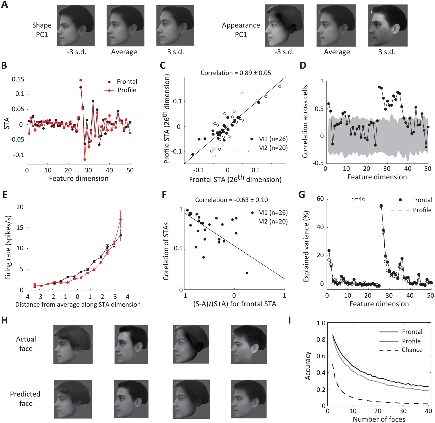
A, To explore how our model could be extended to other views besides frontal, parameterized faces of right profiles were generated whose main dimensions were conjugate to those of the 2000 frontal faces (see STAR Methods). The first PCs for shape features and appearance features of the profile face space are shown (for more PCs see Figure S2E). B, Spike-triggered average computed using 2000 frontal stimuli (black) and 2000 profile stimuli (red) for an example cell in AM. C, Correlation between profile STA and frontal STA on one single feature dimension (1st appearance dimension) across n=46 AM neurons. Solid and open circles indicate data from two different monkeys. D, STA correlation across cells for all 50 dimensions. Shaded regions indicate 99% confidence intervals of randomly shuffled data. E, Response of the neuron in B is plotted against distances between the stimuli and the average face along the STA axis for frontal and profile stimuli. The distance was rescaled so that STA corresponds to 1. Error bars represent s.e. F, The relationship between face view invariance and feature preference for frontal images across cells. Face-view invariance is quantified as the correlation between frontal and profile STA across 50 dimensions for each neuron. The black line indicates linear fit of the data. G, For the set of 4000 faces, including 2000 frontal and 2000 profile faces, we trained a linear model to predict features on individual dimensions based on population responses of 46 AM cells. Explained variances of all 50 feature dimensions are plotted for frontal and profile faces separately. H, Four reconstructions of profile faces based on the predicted features are shown alongside the corresponding faces presented to the monkey. I, Decoding accuracy as a function of the number of faces (solid lines, similar to Figure 3B), using the model in (G), shown separately for frontal and profile faces (either a frontal or a profile face had to be identified from a number of faces of mixed views).
The high correlation in tuning to appearance parameters of profile and frontal faces (Figures 6B–D) suggests that we should be able to decode faces independent of head orientation from AM cell activity. We next decoded feature values of both profile and frontal faces using linear regression on population responses, analogous to Figures 2 and 3. Importantly, for each cell, we used the exact same 51 model parameters to fit responses to both frontal and profile faces (rather than 51 model parameters for frontal faces and 51 different parameters for profile faces), motivated by the high correlation in tuning to appearance parameters of profile and frontal faces (Figures 6B–D). We found we could predict profile faces quite well despite only using 46 cells (Figures 6G and H). To quantify decoding accuracy, we carried out the same analysis as in Figure 3B separately for frontal and profile faces (but using the same model for both). We could identify both frontal and profile faces well above chance (Figures 6I). Overall, these results show that a simple model (namely, linear projection onto a single appearance STA axis) can account for responses of AM cells to facial images across different views.
Computational advantages of an axis metric over a distance metric
Why do ML/MF and AM choose linear projection onto face axes to represent faces? Previous studies have argued that nonlinear mixing of responses to different task variables in a complex task is necessary to generate a high dimensional representation that can then be flexibly read out along multiple dimensions through linear classifiers (Rigotti et al., 2013). In the case of face representation, however, the space is already inherently high dimensional; thus linear encoding could be sufficient. To test this idea, we trained a simple 1-layer neural network to identify one face out of 200 faces (Figure 7A2). The inputs to the network contained 200 units whose tuning to faces was defined by either a nonlinear distance metric (measuring distance from one particular face to the exemplar face) or a linear axis metric (measuring the projection of one face onto the axis). We varied the dimensionality of the input stimulus space, and found that a distance metric performed better than an axis metric for lower dimensionality, but the two were comparably good for dimensionality higher than six (Figure 7A3). Two further simulations demonstrate the advantages of an axis metric. First, axes are more efficient, allowing a smaller number of units to achieve similar performance. When we performed principal component analyses on a set of units tuned to faces according to a distance metric, we found the PCs displayed linear tuning in the space, consistent with an axis metric (Figure 7B1, Figure S6B), indicating the same number of units tuned to axes capture more variability than units using distance. To explicitly compare the efficiency of axis versus distance units, we performed the same analysis as in Figure 7A, but used only 10 input units (Figure 7B2), and found that axis metrics performed better for dimensionality higher than three (Figure 7B3). We can make an analogy to color coding, which can be accomplished either with a large number of cells tuned to specific hues such as periwinkle and chartreuse, or more efficiently, by cells encoding projection onto three axes, R, G, and B. A second advantage of linear tuning is robustness. In the weight matrix of the network trained in Figure 7A using either an axis or a distance metric, the output units of the axis model received more distributed inputs than those of the distance model (Figure 7C1). Linearly pooling inputs with similar signal but independent noise would help improve the signal quality (Figure 7C2), leading an axis model to perform better in noisy conditions. To test this idea, we repeated the same analyses as in Figure 7A, but added a large amount of random noise to the inputs (Figure 7C2, lower). We found that for dimensionality higher than three, axis models perform better than distance models (Figure 7C3). Finally, an axis metric endows downstream areas reading out the activity of AM with greater flexibility to discriminate along a variety of different dimensions. If there is a linear relationship between facial features and responses, then one can linearly decode the facial features (Figure 3) and use these decoded features flexibly for any purpose, not only for face identification (e.g., by “Jennifer Aniston” cells in the hippocampus (Quiroga et al., 2005)), but also other tasks such as gender discrimination or recognition of daily changes in a familiar face (Figure 7D). In sum, axis coding is more flexible, efficient, and robust to noise for representation of objects in a high-dimensional space compared to exemplar coding.
Figure 7. An axis-metric representation is more flexible, efficient, and robust for face identification.
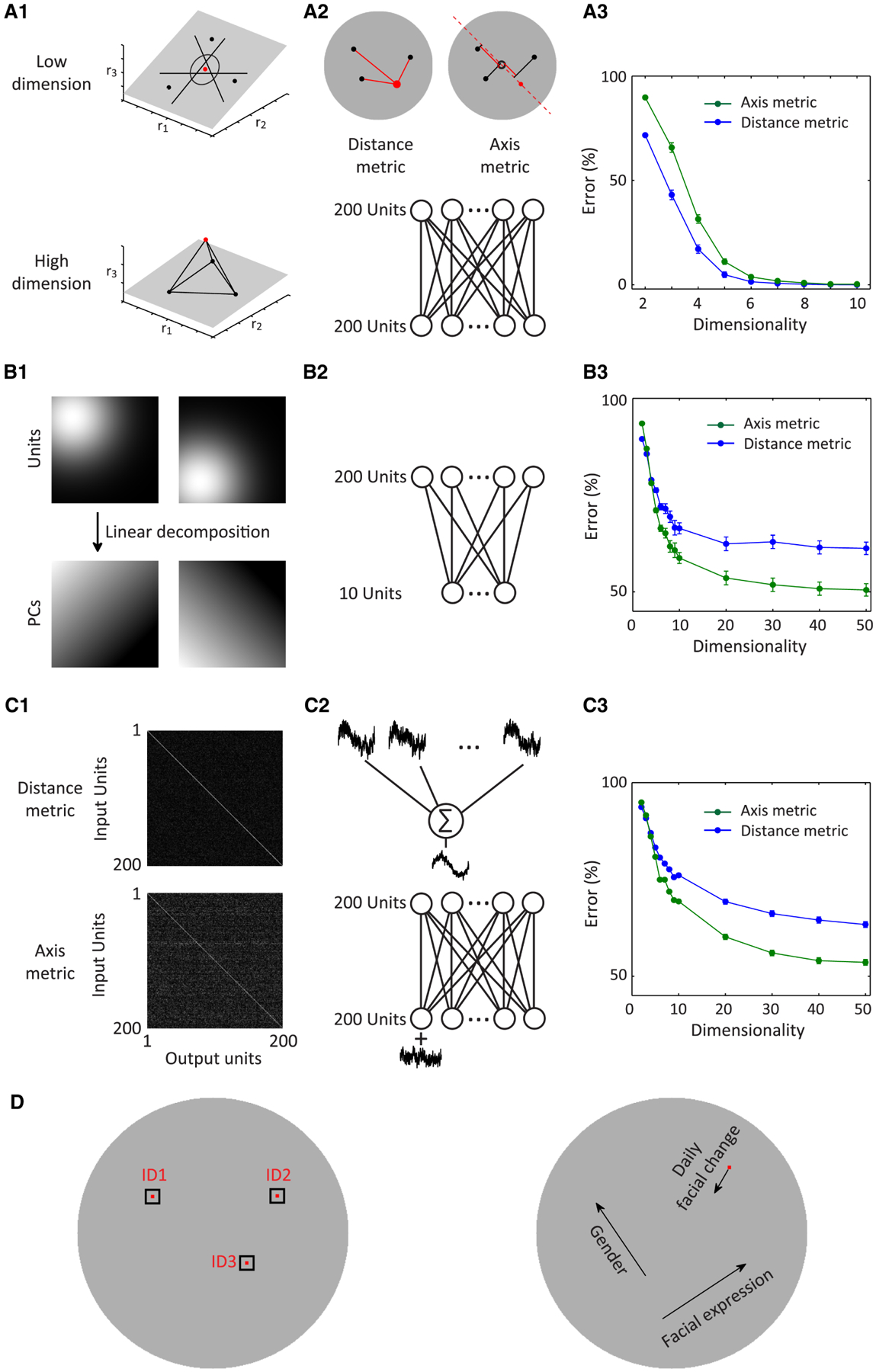
A, An axis metric can perform as well as a distance metric on an identification task for high-dimensional representation but not for low-dimensional representation. A1, For an identification task, a linear classifier is usually non-optimal for a low-dimensional space (upper), e.g., it’s impossible to linearly separate the red dot from the black dots in the same plane, while a circular decision boundary defined by the distance to the red dot could easily perform the task. However, if the representation of these dots were high-dimensional, it’s much easier to separate the dots (lower). A2, We explored how axis and distance metrics (upper) defined on feature spaces of variable dimensions perform in a face identification task. A simple network model (lower) was trained to identify one of the 200 faces based on 200 units with tuning defined by a distance-metric or an axis-metric on a feature space of variable dimensionality. These units used exactly the same 200 faces to be identified to define exemplars/axes of the inputs (red dot in the upper left, and red dashed line in the upper right). A3, Error rate of identification was plotted against dimensionality for both models. B, An axis metric is more efficient than a distance metric. Assume we have model neurons that are tuned in a high-dimensional feature space proportional to the distance to a fixed point. Dimension reduction on a population of such units using principal component analysis reveals that the main PCs are almost linearly tuned in the space (for quantification see Figure S6B). B2 and B3, same as A2 and A3 but using 10 input units. For high dimensionality, axis metrics outperformed the distance metrics. C, Axis metrics are more distributed and more robust to noise than distance metrics. C1, Weight matrices of networks in B after training using units defined by an axis metric or a distance metric (white indicates large weight). Weights for the distance metric are mostly on the diagonal, while those for the axis metric are more distributed. C2, Distributed inputs could help average signals with independent noise, resulting in high signal-to-noise (upper). The same network in A2 was trained with noisy inputs (lower). C3, Error rates of both models plotted against dimensionality. D, The linear relationship between neuronal responses and facial features ensures diverse tasks can be performed. The gray disks indicate face space.
Discussion:
In this paper, we reveal the code for realistic facial identity in the primate brain. We show that it is possible to decode any human face using just ~ 200 face cells from patches ML/MF and AM, once faces are defined in the proper space (as vectors in a “shape-appearance” space). Furthermore, we reveal the mechanism underlying this remarkably efficient code for facial identity: linear projection of incoming face vectors onto a specific axis (the “STA” axis). We find that in planes orthogonal to this preferred axis, cells show completely flat tuning. Surprisingly, even cells that had previously been thought to respond extremely sparsely turned out to have this property; by finding the null plane for these cells, we were able to engineer a large set of faces that all triggered strong responses in these putative “sparse” cells. This is surprising because it means there are no detectors for identities of specific individuals in the face patch system--even though intuitively one might expect this, especially after observing a sparse AM cell (Movie S2). Using the axis code, we could predict firing rates of face cells in response to arbitrary faces close to their noise ceiling. Advantages of axis coding include: efficiency, robustness, flexibility, and ease of readout. Our results demonstrate that at least one subdivision of IT cortex can be explained by an explicit, simple model and “black box” explanations are unnecessary.
Several previous studies have explored tuning of IT cells within a face space framework. Our results are inconsistent with a previous study (which did not specifically target AM) claiming that face representation in anterior IT is mediated by cells showing V-shaped tuning around the average face in face space (Leopold et al., 2006). Our results are consistent with a previous study which showed ramp-like tuning of face cells in ML/MF to geometric features such as inter-eye distance in cartoon faces (Freiwald et al., 2009). However, the current study goes far beyond this previous study, by (1) recording from both AM and ML/MF, (2) testing a large set of parameterized realistic faces rather than cartoon faces, (3) showing that an axis model can be used to accurately decode and encode responses to realistic faces, and (4) most importantly, showing that in both patches, tuning in the hyperplane orthogonal to the preferred axis is flat. The last point is critical: while many coding schemes are consistent with ramp-shaped tuning (Figure S3I), a coding scheme in which tuning is flat in the hyperplane orthogonal to the STA is what turns face cells into linear projection machines. And this is what makes the code for faces so efficient (essentially, a high dimensional analog of the familiar RGB code for colors), allowing realistic faces to be accurately decoded with such a small number of cells.
How are cells wired to transform an object, defined in pixel coordinates, into a shape-appearance feature vector representation? It is possible to automatically extract a shape-appearance feature vector representation of a face image using a stochastic gradient descent algorithm (Blanz and Vetter, 1999). Most likely, in the brain, such a representation is produced by an architecture similar to a hierarchical feedforward deep-network. A variety of biologically-plausible neural networks have been trained to automatically extract key landmark positions from face images (Kumar et al., 2016). Note that the shape-free appearance descriptor could be approximated based on intensity variations around the landmarks (e.g., eye intensities and hair colors)—the original image doesn’t have to be warped in a literal sense. Interestingly, when we analyzed the representation used by units in the final layer of a CNN trained to recognize faces, we found that tuning of these units was more consistent with an axis model than an exemplar model, and furthermore was strongly appearance-biased, resembling AM (Figure S7B–F). The fact that the CNN developed these properties even though it was not explicitly trained to extract appearance coordinates suggests that an axis representation may arise naturally from general constraints on efficient face recognition. Regardless how the wiring is accomplished by the brain, we believe our insight that the brain is formatting faces into a shape/appearance feature vector representation is important in itself (by analogy, grid and place cells have provided deep insight into neural coding of an animal’s spatial environment, even though the mechanism by which these cell types are generated remains heavily debated).
It may seem like a stroke of luck that the axes we chose to generate faces, namely, the 50 shape and appearance axes, turned out to explain responses of ML/MF and AM cells in such a simple way. However, these axes were in fact not arbitrary but meaningful: within the space spanned by these axes, every point corresponds to a realistic face. This is a highly constraining property: in order to achieve this, most algorithms for generating realistic faces use a similar approach, first aligning landmarks and then performing principal components analysis separately on landmark positions and aligned images (Beymer and Poggio, 1996; Blanz and Vetter, 1999; Cootes et al., 2001; Edwards et al., 1998). In contrast, applying principal components analysis on faces directly, without landmark alignment, produces “Eigenfaces” composed of blurry features that do not look like realistic faces (Sirovich and Kirby, 1987; Turk and Pentland, 1991). Of course, enlargement of the stimulus space to include not only human faces but also monkey faces, and not only neutral faces but also expressive faces, would likely add additional axes. Furthermore, the axis representation in AM is likely invariant not only to view but also to other accidental transformations such as clutter, illumination, and partial occlusion. The shape-appearance axis framework proposed here can be readily extended to accommodate these extensions of face space.
Our finding that AM cells are coding axes of shape-free appearance representations rather than “Eigenface” features (Figure 4L) is consistent with a recently proposed explanation for the effectiveness of deep neural networks in image recognition (Lin and Tegmark, 2016): a visual image on the retina can be considered the result of a hierarchical generative model starting from a set of simple variables, e.g., shape-free appearance features. Deep neural networks are reversing this generative hierarchy, one step at a time, to derive these variables at the final layers. According to this view, the reason the brain codes shape and appearance features is that these are the key input variables to the hierarchical generative model for producing face images which the brain has learned to reverse.
We think the insights gained in our study of face representation may shed light on the general problem of object representation. One can imagine applying these same constraints to generate an analogous space for non-face objects and then testing whether non-face objects are also coded by cells representing principal components of a shape space together with a shape-invariant object space. However, the space of non-face objects is far less homogeneous than that of faces, so it may be difficult to register different non-face objects to compute a set of shape and shape-free appearance axes. Configural coding in terms of shape fragments is a third alternative to the holistic axis and exemplar models considered in this paper, and is supported by previous studies showing that general object coding is best described in terms of Gaussian-like tuning for contour, surface, and medial axis fragments in explicitly geometric dimensions like orientation, curvature, and relative position (Brincat and Connor, 2004; Hung et al., 2012).
Regardless of the details of how non-face objects are represented in IT, we believe the computational goal of object representation is likely the same across all of IT including face patches. The present study suggests that within face patches, this goal is to set up a coordinate system to measure faces rather than to explicitly identify faces, since almost every single face cell we recorded was susceptible to face metamers. Given that it is actually trivial to construct metamer-resistant exemplar-tuned units from a set of axis-tuned units (e.g., by applying a softmax function to the output of the latter), it is surprising that we didn’t find any evidence for the former in IT face patches. It seems the brain anatomically parcellates the functions of object measurement and object identification. Future work is needed to clarify the metric coordinate system(s) used by IT to measure objects in general, as well as the mechanisms for explicit object identification that occur after IT.
STAR METHODS:
CONTACT FOR REAGENT AND RESOURCE SHARING
Further information and requests for reagents and resource may be directed to and will be fulfilled by the Lead Contact, Dr. Doris Tsao (dortsao@caltech.edu).
EXPERIMENTAL MODEL AND SUBJECT DETAILS
Two male rhesus macaques (Macaca mulatta) of 7–9 years old were used in this study. Both animals were pair-housed and kept on a 14 hr/10hr light/dark cycle. All procedures conformed to local and US National Institutes of Health guidelines, including the US National Institutes of Health Guide for Care and Use of Laboratory Animals. All experiments were performed with the approval of the Caltech Institutional Animal Care and Use Committee (IACUC). 78 anonymous participants were recruited online (Amazon Turk, https://www.mturk.com/) for the human psychophysics experiment, which was approved by Caltech Institutional Review Board (IRB).
METHOD DETAILS
Face Patch Localization
Two male rhesus macaques were trained to maintain fixation on a small spot for juice reward. Monkeys were scanned in a 3T TIM (Siemens, Munich, Germany) magnet while passively viewing images on a screen. Feraheme contrast agent was injected to improve signal/noise ratio. Face patches were determined by identifying regions responding significantly more to faces than to bodies, fruits, gadgets, hands, and scrambled patterns, and were confirmed across multiple independent scan sessions. Additional details are available in previous publications (Freiwald and Tsao, 2010; Ohayon and Tsao, 2012; Tsao et al., 2006).
Single-unit recording
Tungsten electrodes (18–20 Mohm at 1 kHz, FHC) were back loaded into plastic guide tubes. Guide tubes length was set to reach approximately 3–5 mm below the dura surface. The electrode was advanced slowly with a manual advancer (Narishige Scientific Instrument, Tokyo, Japan). Neural signals were amplified and extracellular action potentials were isolated using the box method in an on-line spike sorting system (Plexon, Dallas, TX, USA). Spikes were sampled at 40 kHz. All spike data was re-sorted with off-line spike sorting clustering algorithms (Plexon). Only well-isolated units were considered for further analysis.
Behavioral Task and Visual Stimuli
Monkeys were head fixed and passively viewed the screen in a dark room. Stimuli were presented on a CRT monitor (DELL P1130). The intensity of the screen was measured using a colorimeter (PR650, Photo Research) and linearized for visual stimulation. Screen size covered 27.7*36.9 visual degrees and stimulus size spanned 5.7 degrees. The fixation spot size was 0.2 degrees in diameter and the fixation window was a square with the diameter of 2.5 degrees. Images were presented in random order using custom software. Eye position was monitored using an infrared eye tracking system (ISCAN). Juice reward was delivered every 2–4 s if fixation was properly maintained.
For visual stimulation, all images were presented for 150 ms interleaved by 150 ms of a gray screen. Each image was presented 3–5 times to obtain reliable firing rate statistics. In this study, four different stimulus sets were used:
A set of 16 real face images, and 80 images of objects from nonface categories (fruits, bodies, gadgets, hands, and scrambled images) (Freiwald and Tsao, 2010; Ohayon and Tsao, 2012; Tsao et al., 2006) (Figure S1).
A set of 2000 images of parameterized frontal face stimuli, generated using the active appearance model (Cootes et al., 2001; Edwards et al., 1998) (Figures 1–4, Figure S2A).
A set of 2000 images of parameterized profile face stimuli (Figure 6, Figure S2E).
A set of 144 images of parameterized frontal face stimuli, generated online using responses of the recorded neuron (Figure 5).
Generation of parameterized face stimuli
We used real face images from an online face database, FEI face database (http://fei.edu.br/~cet/facedatabase.html). This database contains images from 200 individuals with 11 different head orientations (from left full profile to right full profile). Generation of parameterized face stimuli followed the procedure of previous papers on active appearance modeling (Cootes et al., 2001; Edwards et al., 1998): First, a set of 58 landmarks were labeled on each of the frontal face images (Figure 1A). The positions of landmarks were normalized for mean and variance for each of the 200 faces, and an average shape template was calculated. Then each face was smoothly warped so that the landmarks matched this shape template, using a technique based on spline interpolation (Bookstein, 1989). This warped image was then normalized for mean and variance and reshaped to a 1-d vector. Principal component analysis was carried out on positions of landmarks and shape-free intensity independently. The first 25 PCs of landmark positions (“shape” dimensions, both x and y coordinates from all landmarks were concatenated into a 116-d vector) and 25 PCs of shape-free intensity (“shape-free appearance” dimension, intensities of all pixels of the warped images were concatenated into a 17304-d vector) were used to construct a parameterized face space. The distribution of feature values for each PC dimension followed a Gaussian distribution with variance proportional to that of the 200 faces from the database. Then 2000 images were randomly drawn from this space (and constructed from the 50-d feature vector by inverting the process above). Pair-wise correlations between the 2000-long vectors for each dimension were further removed by orthogonalization. The feature values were scaled by two scaling factors (constant across all images), one for appearance features and one for shape features, such that the total variances of shape features and appearance features (sum of variances cross dimensions) were both equal to 0.5, i.e.,
where is the value of shape/appearance feature dimension i in face j, and is the mean value of shape/appearance feature dimension i across all 2000 faces.
For profile stimuli, we repeated the same procedure using images of the same identities from other views, taken from the same database (Figure S2E). To register frontal coordinates with profile coordinates, we projected the 200 frontal faces and 200 profile faces to the 50-d frontal face space and profile face space respectively. The correspondence between frontal coordinates and profile coordinates was identified using linear regression for shape dimensions and appearance dimensions independently; the resulting linear transformation was applied to the profile coordinates, to produce new profile coordinates registered to the frontal coordinates. In detail, we use and to denote the frontal and profile coordinates on the ith feature dimension of the jth identity (note, the are coordinates in the original, unregistered profile face space). For each profile dimension i we carried out the following linear regression:
where are the regression coefficients, and are the error terms. The procedure was carried out for all 50 shape and appearance features independently. In this way, for each face in the frontal face space, we could compute optimal coordinates in the unregistered profile face space of the profile face of the same individual. Then, to obtain coordinates of this same profile face in the registered profile face space, we simply used the frontal coordinates to denote it. For example, the profile face with coordinates (1 0 0 … 0) in the registered profile face space would be the face with coordinates in the unregistered profile face space. We repeated the same procedure for images in other views, generating 9 views altogether for each identity (Figure S2F; only full left profiles were used for Figure 6, while all views were used for Figure S7).
Human psychophysics
To quantify subjective similarity between the reconstructed faces and the actual faces, responses from 78 human participants were collected from Amazon’s Mechanical Turk (https://www.mturk.com/). All participants signed an electronic consent form at the beginning of the experiment. In each trial, two faces were randomly drawn from the stimulus set, and one of them was reconstructed based on the population responses of all face cells. The face corresponding to the reconstruction was considered as the target and the other one was considered as the distractor. The participant had to report which of the two faces was more similar to the reconstruction. This design is comparable to the case of two faces in the “objective” quantification of decoding accuracy (Figure 3B, see below). The average accuracy of human subjects was 88.3%, significantly above chance (p=6*10−62, one-sample t-test). We were also interested in human decoding accuracy under more difficult conditions, specifically the case of 40 faces. It is impractical to present 40 faces to the human subject at the same time, so we designed a new experiment to mimic the case of 40 faces. In this experiment, we selected the “distractor” face in the following way: 39 faces different from the “target” face were randomly drawn from the stimulus set, and the one with the smallest face-space distance to the reconstructed face was chosen as the distractor. This task is similar to the “objective” quantification of decoding accuracy using 40 faces (Figure 3B), in the sense that the comparison of similarity performed by the human subject is the same critical comparison performed by the algorithm determining the “objective” (distance-based) decoding accuracy: if the actual face is considered to be more similar to the reconstructed face than the face that is the most similar one to the reconstructed face out of the 39 faces, it should be considered the one out of 40 faces most similar to the reconstruction. We found that in this much more difficult face identity matching task, human performance remained significantly better than chance (average=69.6%, p=6*10−24, one-sample t-test). Similar to a previous report (Cowen et al., 2014), the subjective (human-based) decoding accuracy was lower than the objective (distance-based) decoding accuracy, likely due to noise in the decision making process of human participants.
QUANTIFICATION AND STATISTICAL ANALYSIS
Face selectivity index
To quantify the face selectivity of individual cells, we defined a face-selectivity index as
| (1) |
The number of spikes in a time window of 50–300 ms after stimulus onset was counted for each stimulus. Units with high face selectivity (FSI>0.33) were selected for further recordings.
Spike triggered average analysis
The number of spikes in a time window of 50–300 ms after stimulus onset was counted for each stimulus. To estimate the spike-triggered average (STA), the 50-d stimulus vector was multiplied by the spike number and averaged across the stimuli presented:
| (2) |
where f(n) is the spiking response to the nth stimulus, and is the vector representing the nth stimulus.
To estimate neuronal preference for shape or appearance features, we first computed the vector length for the shape dimensions of the STA (suppose , shape STA vector length=|(A1,⋯,A25)| and appearance STA vector length = |(A26,⋯,A50)|, using Euclidean distance). The shape preference index was defined as:
| (3) |
where S and A are vector lengths for shape and appearance STAs.
To test the reliability of our analysis, we randomly split the 2000 images into two halves, and computed shape preference index for each half. We found shape preference indices were highly correlated in independent data sets (correlation=0.89±0.07, n=205 cells).
Statistical significance of tuning along a single axis in the face space
To quantify the significance of the tuning along an axis, we first shifted spike trains by a random amount of time and then computed tuning along the axis in the following way (see also Figures 1 J and K): we first rescaled the axis so that [−1 1] contains 98% of all 2000 projections, then grouped the features between [−1 1] into 16 equidistant bins and computed the average response for each bin; s.d. of 16 average responses was used to quantify the strength of tuning (i.e., how inhomogeneous the response is). The same procedure of random shifting was repeated 1000 times. The tuning was considered significant if the strength of tuning was higher than 990 random shifts (p<0.01).
Decoding analysis
Population responses from neurons in AM or ML/MF to 2000 facial images generated by the active appearance model were used to decode 50-d features. Leave-1-out cross validation was employed:
Population responses to 1999 images were used to predict feature values by linear regression,
| (4) |
where fij is the feature value of the ith image on the jth dimension, is the response of the nth neuron to ith image, are the regression coefficients. This linear model was then tested on the remaining image.
Fitting quality of the model was determined by the percentage of variance in data explained by the model (R2):
| (5) |
where yi is the observed data, fi is the model fit, is the mean of the observed data.
To quantify the overall decoding accuracy of the model, we randomly selected a number of faces from the stimulus set of 2000 faces and compared their actual 50-d feature vectors to the reconstructed feature vector of one face in the set using Euclidean distance. If the actual face with the smallest distance is the face corresponding to the reconstruction, the decoding is considered correct. We repeated the procedure 1000 times to estimate the accuracy.
Linear regression was used for decoding most of the time. Two additional methods were considered: Nearest neighbor finds the stimulus in the 1999 training set that has the closest distance to the test stimulus in the space of neuronal responses (in this space, each dimension represents the response of one neuron); Nearest K-neighbor finds K-stimuli of the 1999 training set that are closest to the test stimulus, and computes the average of the K-stimuli as the prediction.
To test the reliability of decoding performance, a bootstrap procedure was employed (Jiang et al., 2008): a bootstrap sample of 2000 images was randomly drawn with replacement from the original stimulus set. We then applied a cross-validation procedure on this bootstrap sample. That is, to predict features of one image, we left out all the replications of this image in the bootstrap sample and used what remained to train the linear model for prediction. Decoding accuracy was then estimated for each bootstrap. Standard deviations and confidence intervals of decoding accuracy were then computed from 1000 iterations of bootstrapping.
To compare decoding accuracy between neuronal populations, the same number of neurons (n=99) were randomly drawn with replacement from both populations. Decoding accuracy was estimated for each random sampling. The p-value of null hypothesis was determined by comparing decoding accuracies from 1000 iterations of such random sampling.
Computation of neuronal tuning along axis orthogonal to STA
For each neuron tested with 2000 parameterized facial images, the STA was first computed. Since there were many axes orthogonal to STA, we cannot sample all of them. Thus we wanted to measure tuning along long axes, i.e., the axes that account for largest variability of the images’ coordinates in the 50-d space, so that tuning could be most reliably fitted. Two different approaches were employed. 1) We randomly selected 2000 axes, and orthogonalized them to the STA. We then sorted the orthogonal axes according to the variability of images explained, and the top 300 axes were chosen. Average tuning along 300 axes was computed. 2) We first orthogonalized 2000 faces to STA, and then used PCA to extract the axis accounting for the largest variability of 2000 orthogonalized faces. Tuning along this “longest axis” was computed.
After tuning of each neuron was computed, we fitted a Gaussian function () to each tuning curve, and used the ratio of the fit at the surround (x=0.67) and the center(x=0) to quantify nonlinearity of tuning.
Two control models were generated to compare with AM neurons. 1) Exemplar model: for each unit, we first selected one of the 200 real faces projected onto 50-d face space as an “exemplar” face, and the response of this unit to any face was set to be a decreasing linear function of the distance between this face and the exemplar in 50-d face space. Therefore a face closer to the exemplar will evoke larger response. Alternatively we randomly chose extreme faces with vector lengths of 2 (larger than any of the real faces) as “exemplars”, to account for the possibility that units seeming to use an axis code might actually be using extreme exemplars. 2) Max-pooling model: for each unit, we first generated 81 transforms of one identity (9 views*9 positions, Figure S2F) in the face space. Then we defined the similarity between any facial image and one of the transforms using a decreasing linear function of the mean absolute difference in pixel intensities between two images, so that a smaller intensity difference would result in higher similarity. The response of the unit to any face was set to the maximum of its similarity to all 81 transforms.
To make a fair comparison between AM neurons and the control model units, we matched the model units to the actual AM neurons in both sparseness and noise. Sparseness of neuronal responses was computed in the following way:
| (6) |
where N=2000, and Ri is the response to ith image. Lower values indicate sparser responses.
It was important to match sparseness of model units to the real units, because sparseness can make a nonlinearity appear stronger (e.g., see the green dots in Figure 4F: sparser cells show more nonlinear, bell-shaped tuning). It was furthermore important to match noise of model units to real units, because noise could change the sparseness (e.g., a constant distribution is the least sparse distribution, while adding noise to it will increase the sparseness), which would in turn affect the apparent nonlinearity of tuning. Thus we added two further components to the modeled response, a threshold and Gaussian noise, and controlled these two parameters so that both sparseness and noise for each simulated unit was matched to one of the AM neurons. Noise for neurons was estimated using bootstrapping; for each neuron, bootstrap samples were created for each image: responses to different repetitions of one image were randomly drawn with replacement, and the average response was computed for each sample. The s.d. of the average responses was determined for each image and averaged across 2000 images to yield the noise for each neuron. We divided this noise by the s.d. of the average responses to the 2000 images (i.e., the signal) to generate a scale-free definition of noise. For the model units, we added random noise to the responses of each unit; we then computed the s.d. of these responses for a single image, averaged across all images, and divided noise by the s.d. of the responses to 2000 images to obtain the overall noise estimate, just as we did for the real neurons.
Model fitting
To quantify which model better predicts neuronal responses, we repeated a small subset of 100 stimuli 10 times more frequently that the rest of the 1900 stimuli. We used the 1900 stimuli as the training set to fit one of the following two models, and used the 100 stimuli to validate the model.
Both models started from 50-d representation of faces. Model 1 (axis model) assumed the 50-d features are first combined linearly and then passed through a third order polynomial. All coefficients of linear fitting and the polynomials were considered parameters and adjusted by gradient descent to minimize the error of fit. Model 2 (exemplar model) assumed the Euclidean distance between the 50-d features and an “exemplar” face is computed and then passed through a third order polynomial. The 50-d features of the exemplar face and coefficients of the polynomial were considered as parameters in this case. We restricted the vector length of the exemplar face to be smaller than 2 to avoid very extreme exemplar faces. Faces with vector length of 2 already look quite extreme (Figure S2D), and the projections of the 200 real faces from the database all had vector length <2 (Figure S2C2), so the restriction is reasonable. The percentage variance of responses to 100 faces explained by each model was used to quantify the quality of fit.
Neural network modeling
1-layer neural networks were trained to identify faces: inputs were simulated responses of different models to one of 200 faces, and the outputs were 200 units representing 200 identities. Distance metric units used the Euclidean distance between one face and the exemplar face as inputs, while axis metric units used the projection onto the axis containing the exemplar face as inputs. The dimensionality of the feature space, where distance and projection were computed, was systematically varied: we sorted the 50 dimensions according to variance, and used the top n dimensions as the axes of the n- dimensional feature space. For each image, activations of the input units were normalized to 0 mean and unit variance to facilitate training. Gradient descent was used to minimize a softmax loss function, and we updated parameters until the network converged.
Two levels of noise were added to the inputs. Low noise level (Figures 7A and B): random Gaussian noise with s.d. =0.6*s.d. of inputs; high noise level (Figure 7C): random Gaussian noise with s.d.=2.4*s.d. of inputs. Noise was linearly added to the inputs of the network. Nine trials of noise implementation were used to train the network and one other trial was used to test the performance of the trained model.
Convolutional neural network modeling
We implemented a convolutional neural network using an online package (MatConvNet, http://www.vlfeat.org/matconvnet). The input images had size of 100*100, containing faces of 500 individuals at 9 views and 9 positions (Figure S2F). The first two hidden layers were convolutional layers, which included both linear convolution and max pooling. The same linear convolution was replicated across the whole image. The size of linear convolution for both layers was 15*15 and the size of max pooling was 4*4. The convolutional layers were followed by two fully connected layers with rectified linear units in between. The number of features after each layer was: 20, 50, 200 and 500. The output identity of the network was the unit in the final layer with maximum value. A softmax loss function was added to the final layer for training. The network was trained to output the correct identity irrespective of view and position. After training, the network reached nearly perfect performance, with validation error <1%. The 2000 parameterized facial images were then loaded to the network to investigate the representation of face space in the final layer of the network (before softmax loss function).
Online generation of facial images based on the responses of face cells
After recording a face cell’s responses to the 2000 parameterized frontal faces, STA stimuli were computed. We then determined the principal orthogonal axis in the following way: 25-d appearance features of 2000 faces were orthogonalized to the STA to produce 2000 STA-orthogonal feature vectors, and PCA was performed to extract the axis accounting for the largest variability among the 2000 STA-orthogonal feature vectors. 12 feature values were evenly sampled from both the STA axis and the principal orthogonal axis, extending from −1.2 to 1.2 (here, 1=the average norm of 2000 faces), and 12*12 images were generated according to each pair of feature values. For Figure 5C, we repeated the above procedure for the second principal orthogonal axis.
DATA AND SOFTWARE AVAILABILITY
All data are available upon request to the Lead Contact.
Supplementary Material
Figure S1. Localization of face patches, Related to Figure 1.
A, Sagittal slices showing location of fMRI-identified face patches in one monkey targeted for recording; dark black line indicates electrode. B, Neuronal responses (baseline-subtracted, averaged from 50 to 300 ms) to images of different categories recorded from the middle face patches (ML/MF, left) and the anterior face patch AM (right). C, Distribution of face selectivity index (FSI) across all visually-responsive neurons. Dotted lines indicate |FSI|=0.33.
Figure S2. Feature dimensions of parameterized face stimuli, Related to Figure 1.
A, Frontal faces corresponding to the first 3 PCs for shape (top) and first 3 PCs for shape-free appearance (bottom). B, Original faces from the database are shown alongside reconstructions based on their feature values in the 50-d space. C1, Gray lines show distribution of feature values of 200 real faces along 50 dimensions, normalized to zero mean and unit variance. Black line shows prediction by standard Gaussian distribution. C2, Sorted vector lengths of 200 real faces in 50-d feature space. C3, Sorted vector lengths of 2000 parameterized faces in 50-d feature space. D, Example parameterized faces with twice the vector length of the average of actual faces. E, The same as (A), but for profile faces. F, Parameterized facial images of the same identity at 9 different views. G, The first 9 Eigenface feature dimensions. The intensity was normalized so that 0 was mapped to middle gray, and maximum absolute value was mapped to black or white.
Figure S3. Tuning along single axis orthogonal to STA is flatter for AM neurons than control models using exemplars or max pooling, Related to Figure 4.
A, Tuning of 99 AM cells along the single axis orthogonal to STA in 25-d appearance feature space that accounts for the most variability. Red dot and error bar represent mean and s.d. B, Same as A, but for models using distance to an exemplar face to compute responses (c.f. Figure 4B). Sparseness and noise levels are matched to AM cells. C, Same as B, but using extreme faces as exemplars of each cell (vector length=twice the average of real faces). D, Same as B, but using max pooling model in Figure 4B. E, The strength of nonlinearity, quantified by the ratio between surround and center of the Gaussian fit (c.f. Figure 4F), is plotted against sparseness for AM and 3 models. Boxes and error bars represent mean and s.e. for three sparseness levels. F, Same as E, but for the absolute difference between the ratio and 1. G and H, Same as E and F, but for all 300 random axes used in Figure 4A. I, Ramp-shaped tuning along STA axis does not imply flat tuning along orthogonal axes. I1, The axis model shows ramp-shaped tuning along STA axis and flat tuning along orthogonal axes. I2, Different examples with ramp-shaped tuning along STA axis (Face axis 1). Only the left-most example shows flat tuning along the orthogonal axis (Face axis 2).
Figure S4. Additional analyses of tuning along axes orthogonal to STA, Related to Figure 4.
A-H, The actual face space spanned by AM cells constitutes a subspace of the 50-d feature space. One concern is that the flat tuning we observed in the orthogonal plane is due to contribution from dimensions which do not modulate any cells in the population. To address this, the actual face space encoded by AM cells was constructed by performing principal component analysis on axes defined by the STAs of appearance-preferring AM neurons. This figure shows that tuning along axes orthogonal to STA is flatter for AM neurons than control models within this actual face space encoded by AM cells. A, To estimate the actual space encoded by AM neurons, we first computed the STA for each neuron, normalized it to norm of 1. To avoid a non-zero mean, we pooled both STAs and their opposite (–STA), then performed principal component analysis on STAs (and –STAs) of all the appearance-biased AM neurons. B, Principal components (PCs) were used to define the axes of the new space. C, The eigenvalue of each PC was used to define a scaling factor of that axis: Larger eigenvalues correspond to longer axes. The gray area indicates 99% confidence interval computed by randomly shuffling the 2000 stimuli. The STA of the randomly shuffled response was rescaled using the norm of the actual STA. The first 47 PCs are significant. For another way of estimating dimensionality of face space using an identification task, see Figure S6A. D-G, same as Figures 4A,B and F, but using distance and orthogonality estimated by the metrics of the new space. H, The absolute difference between 1 and the ratio in G was plotted against sparseness for all three populations. I-L, Another concern is that exemplar cells may use a distance function weighing some dimension more strongly than other dimensions, resulting in non-circular contour lines. Such cells would display flatter tuning along some dimensions than others. We explore this possibility by varying the aspect-ratio between weights of distance along the STA axis and orthogonal axes. I-K, Tuning along axes orthogonal to STA for three aspect-ratios, same convention as Figure 4B. L, Nonlinearity of tuning along orthogonal dimensions for three sparseness levels, as quantified in Figure 4F, were plotted for exemplar cells using distance metrics with different aspect-ratios and AM. Tuning of AM cells are flatter than exemplar cells with aspect ratio as high as eight (p<0.01, Student’s t-test). M and N, Tuning along axes orthogonal to the STA is flatter for ML/MF neurons than the exemplar model in the space of shape features. M, same as Figure 4A, but for tuning of 106 ML/MF cells along axes orthogonal to STA in 25-d space of shape features. N, same as Figure 4F, but for ML/MF cells.
Figure S5. Adaptation plays little role in shaping responses of AM cells, Related to Figure 4.
A, Tuning functions along the STA dimension for an example cell in AM are shown under three adaptation conditions: all trials (blue); trials preceded by a stimulus far from the average face along the STA dimension (33% largest distances, green); trials preceded by a stimulus close to the average face along STA dimension (33% smallest distances, red). The ratio of average distance between the far and near groups was 7.06 on average, thus the two groups represent clearly different adaptation conditions. B, The average tuning function along the STA dimension for 47 AM cells for the three conditions are shown. The response of each cell was normalized to have an average of 1. Error bars represent s.e. Note that we have 47 AM cells in this case, rather than 99 cells, because for 52 cells the presented stimuli included not only frontal faces (e.g., profile faces), making it difficult to collect enough consecutive trials of frontal faces for this analysis. C, Average response to near stimuli (33% smallest distances) was not affected by the distance of the preceding stimulus to the average face (near or far). D, Similar to C, but only considering trials preceded by two consecutive near or far stimuli, which should result in stronger adaptation effect, if there is any. E-H, similar to A-D, but for tuning along axes orthogonal to the STA. Note that distance to the average face was computed along orthogonal axes (c.f. Figure 4A). Error bars represent s.d. There is no significant difference between the two groups in C,D,G and H (p>0.05, paired t-test).
Figure S6. Additional analyses of neuronal dimensionality and linear encoding, Related to Figure 7.
A, To determine the number of dimensions spanned by STAs of AM cells that are useful for performing a face identification task, we first constructed simulated units using the axis model: each unit corresponds to an axis defined by the STA of one AM neuron; sparseness and noise level was set to match that neuron (same as Figure 4B). Note that use of simulated units was important to remove any nonlinearities that might boost task performance independent of the number of linear dimensions spanned by the STAs of the AM cells. Principal component analysis was performed on population responses of 99 simulated cells to 2000 faces. The first n PCs with highest explained variability were used to train an SVM model to identify one face from a total of 200 faces. The SVM model was trained and tested on simulated population responses with noise. Error rate was plotted against number of PCs used. Gray area indicates 99% confidence interval of classification error using 23 PCs (number of dimensions with minimal error) by 1000 iterations of bootstrapping. Error first decays with increasing number of PCs, remaining significant for 17 PCs, suggesting the significant dimensionality of simulated “axis” units’ responses is no less than 18. B, A population of 2000 simulated neurons was constructed using a distance metric in 50-d face space (c.f. Figure 7B1). PCA was performed on the population responses to 2000 faces. Response of the units and PCs were fitted by linear combination of 50-d features and the explained variance was used to quantify linearity of the representation on the space. Unlike the distance units, the first 40 PCs were very well fit by linear combinations of features; in other words, the PCs correspond to axis units. B1, Explained variances for the first 100 (out of 2000) units and first 100 PCs are shown. B2, 100 highest explained variances for units and PCs. None of the 2000 units could be as well fit by a linear model as the top PCs.
Figure S7. Convolutional neural net trained for view-invariant identification supports axis coding, Related to Figure 4.
A, Architecture of convolutional neural network. Two convolution/max pooling layers are followed by two fully connected layers. Inputs were images of 500 identities, each at 9 views and 9 positions. The output compares the features of the 500 units in the final layer and determines the identity in the image. B, After training, 2000 parameterized facial images were loaded to the network, and the STA for each unit was computed. The distribution of feature preference indices for the final layer are shown alongside the distribution for AM and ML/MF. C, Same as Figure 4A, but for the final layer of the convolutional neural network. Sparseness and noise were matched to AM neurons. D, The strength of nonlinearity, quantified by the ratio between surround and center of the Gaussian fit (c.f. Figure 4F), is plotted against sparseness for the final layer of the neural network and two other models (same as Figure 4). Box and error bar represent mean and s.e. for three sparseness levels. E, Same as D, but for the absolute difference between the ratio and 1. F, Responses of units in the final layer were fitted either by an “axis” model or an “exemplar” model (Figure 4G). Percentage explained variance by each model are plotted against each other. The axis model explained a high percentage of variance of unit responses (mean=80.0%), significantly higher than the exemplar model (mean=67.5%, p<0.001, Student’s t-test). This is surprising since we did not give any information to the network about face space axes; one might have expected each output unit to show spherical tuning around each of the 500 target faces, given that the job of each output unit was to identify one of the 500 target faces.
Movie S1. Shape and appearance transformations. Related to Figure 1.
This movie shows a face undergoing only changes in shape parameters, and a face undergoing changes only in appearance parameters.
Movie S2. View-invariant sparse AM neuron. Related to Figure 4.
This movie shows responses of a cell in AM to a set of images. The clicks represent the spikes fired by the cell. This cell responded to only one identity, invariant to head orientation.
Highlights:
Facial images can be linearly reconstructed using responses of ~200 face cells
Face cells display flat tuning along dimensions orthogonal to the axis being coded
The axis model is more efficient, robust and flexible than the exemplar model
Face patches ML/MF and AM carry complementary information about faces
Acknowledgments:
This work was supported by 1R01EY019702, the Howard Hughes Medical Institute, the Tianqiao and Chrissy Chen Institute for Neuroscience at Caltech, and the Swartz Foundation (fellowship to LC). We thank Nicole Schweers for technical support, members of the Tsao lab, Margaret Livingstone, and Albert Tsao for critical comments, and Rodrigo Qian Quiroga for an inspiring conversation.
Footnotes
Publisher's Disclaimer: This is a PDF file of an unedited manuscript that has been accepted for publication. As a service to our customers we are providing this early version of the manuscript. The manuscript will undergo copyediting, typesetting, and review of the resulting proof before it is published in its final citable form. Please note that during the production process errors may be discovered which could affect the content, and all legal disclaimers that apply to the journal pertain.
References:
- Beymer D, and Poggio T (1996). Image representations for visual learning. Science 272, 1905–1909. [DOI] [PubMed] [Google Scholar]
- Blanz V, and Vetter T (1999). A morphable model for the synthesis of 3D faces. Comp Graph, 187–194. [Google Scholar]
- Bookstein FL (1989). Principal Warps - Thin-Plate Splines and the Decomposition of Deformations. Ieee T Pattern Anal 11, 567–585. [Google Scholar]
- Brincat SL, and Connor CE (2004). Underlying principles of visual shape selectivity in posterior inferotemporal cortex. Nat Neurosci 7, 880–886. [DOI] [PubMed] [Google Scholar]
- Cootes TF, Edwards GJ, and Taylor CJ (2001). Active appearance models. Ieee T Pattern Anal 23, 681–685. [Google Scholar]
- Cowen AS, Chun MM, and Kuhl BA (2014). Neural portraits of perception: reconstructing face images from evoked brain activity. Neuroimage 94, 12–22. [DOI] [PMC free article] [PubMed] [Google Scholar]
- Edwards GJ, Taylor CJ, and Cootes TF (1998). Interpreting face images using Active Appearance Models. Automatic Face and Gesture Recognition - Third Ieee International Conference Proceedings, 300–305. [Google Scholar]
- Freiwald WA, and Tsao DY (2010). Functional compartmentalization and viewpoint generalization within the macaque face-processing system. Science 330, 845–851. [DOI] [PMC free article] [PubMed] [Google Scholar]
- Freiwald WA, Tsao DY, and Livingstone MS (2009). A face feature space in the macaque temporal lobe. Nat Neurosci 12, 1187–1196. [DOI] [PMC free article] [PubMed] [Google Scholar]
- Grimaldi P, Saleem K, and Tsao D (2016). Anatomical connections of the functionally- defined “face patches” in the macaque monkey. Neuron 90, 1325–1342. [DOI] [PMC free article] [PubMed] [Google Scholar]
- Hung CC, Carlson ET, and Connor CE (2012). Medial axis shape coding in macaque inferotemporal cortex. Neuron 74, 1099–1113. [DOI] [PMC free article] [PubMed] [Google Scholar]
- Ito M, Tamura H, Fujita I, and Tanaka K (1995). Size and position invariance of neuronal responses in monkey inferotemporal cortex. J Neurophysiol 73, 218–226. [DOI] [PubMed] [Google Scholar]
- Jiang W, Varma S, and Simon R (2008). Calculating confidence intervals for prediction error in microarray classification using resampling. Statistical applications in genetics and molecular biology 7, Article8. [DOI] [PubMed] [Google Scholar]
- Kay KN, Naselaris T, Prenger RJ, and Gallant JL (2008). Identifying natural images from human brain activity. Nature 452, 352–355. [DOI] [PMC free article] [PubMed] [Google Scholar]
- Kumar A, Rangjan R, Patel V, and Chellappa R (2016). face alignment by local deep descriptor regression. arXiv 1601.07950. [Google Scholar]
- Leopold DA, Bondar IV, and Giese MA (2006). Norm-based face encoding by single neurons in the monkey inferotemporal cortex. Nature 442, 572–575. [DOI] [PubMed] [Google Scholar]
- Lin H, and Tegmark M (2016). Why does deep and cheap learning work so well? arXiv. [Google Scholar]
- Majaj NJ, Hong H, Solomon EA, and DiCarlo JJ (2015). Simple Learned Weighted Sums of Inferior Temporal Neuronal Firing Rates Accurately Predict Human Core Object Recognition Performance. The Journal of neuroscience : the official journal of the Society for Neuroscience 35, 13402–13418. [DOI] [PMC free article] [PubMed] [Google Scholar]
- Moeller S, Freiwald WA, and Tsao DY (2008a). A direct link between face-selective regions in temporal and prefrontal cortex. Paper presented at: Society for Neuroscience Conference (Washington D.C.). [Google Scholar]
- Moeller S, Freiwald WA, and Tsao DY (2008b). Patches with links: a unified system for processing faces in the macaque temporal lobe. Science 320, 1355–1359. [DOI] [PMC free article] [PubMed] [Google Scholar]
- Nestor A, Plaut DC, and Behrmann M (2016). Feature-based face representations and image reconstruction from behavioral and neural data. Proc Natl Acad Sci U S A 113, 416–421. [DOI] [PMC free article] [PubMed] [Google Scholar]
- Ohayon S, and Tsao DY (2012). MR-guided stereotactic navigation. J Neurosci Methods 204, 389–397. [DOI] [PMC free article] [PubMed] [Google Scholar]
- Quiroga RQ, Reddy L, Kreiman G, Koch C, and Fried I (2005). Invariant visual representation by single neurons in the human brain. Nature 435, 1102–1107. [DOI] [PubMed] [Google Scholar]
- Riesenhuber M, and Poggio T (1999). Hierarchical models of object recognition in cortex. Nat Neurosci 2, 1019–1025. [DOI] [PubMed] [Google Scholar]
- Rigotti M, Barak O, Warden MR, Wang XJ, Daw ND, Miller EK, and Fusi S (2013). The importance of mixed selectivity in complex cognitive tasks. Nature 497, 585–590. [DOI] [PMC free article] [PubMed] [Google Scholar]
- Schwartz O, Pillow JW, Rust NC, and Simoncelli EP (2006). Spike-triggered neural characterization. J Vis 6, 484–507. [DOI] [PubMed] [Google Scholar]
- Sinha P, Balas B, Ostrovsky Y, and Russell R (2006). Face recognition by humans: Nineteen results all computer vision researchers should know about. P Ieee 94, 1948–1962. [Google Scholar]
- Sirovich L, and Kirby M (1987). Low-Dimensional Procedure for the Characterization of Human Faces. Journal of the Optical Society of America a-Optics Image Science and Vision 4, 519–524. [DOI] [PubMed] [Google Scholar]
- Tanaka K (1996). Inferotemporal cortex and object vision. Annual review of neuroscience 19, 109–139. [DOI] [PubMed] [Google Scholar]
- Tsao DY, Freiwald WA, Knutsen TA, Mandeville JB, and Tootell RB (2003). Faces and objects in macaque cerebral cortex. Nat Neurosci 6, 989–995. [DOI] [PMC free article] [PubMed] [Google Scholar]
- Tsao DY, Freiwald WA, Tootell RB, and Livingstone MS (2006). A cortical region consisting entirely of face-selective cells. Science 311, 670–674. [DOI] [PMC free article] [PubMed] [Google Scholar]
- Tsao DY, Moeller S, and Freiwald WA (2008). Comparing face patch systems in macaques and humans. Proc Natl Acad Sci U S A 105, 19514–19519. [DOI] [PMC free article] [PubMed] [Google Scholar]
- Turk MA, and Pentland AP (1991). Face Recognition Using Eigenfaces. 1991 Ieee Computer Society Conference on Computer Vision and Pattern Recognition, 586–591. [Google Scholar]
- Valentine T (1991). A unified account of the effects of distinctiveness, inversion, and race in face recognition. The Quarterly journal of experimental psychology A, Human experimental psychology 43, 161–204. [DOI] [PubMed] [Google Scholar]
- Vogels R (2016). Sources of adaptation of inferior temporal cortical responses. Cortex; a journal devoted to the study of the nervous system and behavior 80, 185–195. [DOI] [PubMed] [Google Scholar]
- Yamins DL, Hong H, Cadieu CF, Solomon EA, Seibert D, and DiCarlo JJ (2014). Performance-optimized hierarchical models predict neural responses in higher visual cortex. Proc Natl Acad Sci U S A 111, 8619–8624. [DOI] [PMC free article] [PubMed] [Google Scholar]
Associated Data
This section collects any data citations, data availability statements, or supplementary materials included in this article.
Supplementary Materials
Figure S1. Localization of face patches, Related to Figure 1.
A, Sagittal slices showing location of fMRI-identified face patches in one monkey targeted for recording; dark black line indicates electrode. B, Neuronal responses (baseline-subtracted, averaged from 50 to 300 ms) to images of different categories recorded from the middle face patches (ML/MF, left) and the anterior face patch AM (right). C, Distribution of face selectivity index (FSI) across all visually-responsive neurons. Dotted lines indicate |FSI|=0.33.
Figure S2. Feature dimensions of parameterized face stimuli, Related to Figure 1.
A, Frontal faces corresponding to the first 3 PCs for shape (top) and first 3 PCs for shape-free appearance (bottom). B, Original faces from the database are shown alongside reconstructions based on their feature values in the 50-d space. C1, Gray lines show distribution of feature values of 200 real faces along 50 dimensions, normalized to zero mean and unit variance. Black line shows prediction by standard Gaussian distribution. C2, Sorted vector lengths of 200 real faces in 50-d feature space. C3, Sorted vector lengths of 2000 parameterized faces in 50-d feature space. D, Example parameterized faces with twice the vector length of the average of actual faces. E, The same as (A), but for profile faces. F, Parameterized facial images of the same identity at 9 different views. G, The first 9 Eigenface feature dimensions. The intensity was normalized so that 0 was mapped to middle gray, and maximum absolute value was mapped to black or white.
Figure S3. Tuning along single axis orthogonal to STA is flatter for AM neurons than control models using exemplars or max pooling, Related to Figure 4.
A, Tuning of 99 AM cells along the single axis orthogonal to STA in 25-d appearance feature space that accounts for the most variability. Red dot and error bar represent mean and s.d. B, Same as A, but for models using distance to an exemplar face to compute responses (c.f. Figure 4B). Sparseness and noise levels are matched to AM cells. C, Same as B, but using extreme faces as exemplars of each cell (vector length=twice the average of real faces). D, Same as B, but using max pooling model in Figure 4B. E, The strength of nonlinearity, quantified by the ratio between surround and center of the Gaussian fit (c.f. Figure 4F), is plotted against sparseness for AM and 3 models. Boxes and error bars represent mean and s.e. for three sparseness levels. F, Same as E, but for the absolute difference between the ratio and 1. G and H, Same as E and F, but for all 300 random axes used in Figure 4A. I, Ramp-shaped tuning along STA axis does not imply flat tuning along orthogonal axes. I1, The axis model shows ramp-shaped tuning along STA axis and flat tuning along orthogonal axes. I2, Different examples with ramp-shaped tuning along STA axis (Face axis 1). Only the left-most example shows flat tuning along the orthogonal axis (Face axis 2).
Figure S4. Additional analyses of tuning along axes orthogonal to STA, Related to Figure 4.
A-H, The actual face space spanned by AM cells constitutes a subspace of the 50-d feature space. One concern is that the flat tuning we observed in the orthogonal plane is due to contribution from dimensions which do not modulate any cells in the population. To address this, the actual face space encoded by AM cells was constructed by performing principal component analysis on axes defined by the STAs of appearance-preferring AM neurons. This figure shows that tuning along axes orthogonal to STA is flatter for AM neurons than control models within this actual face space encoded by AM cells. A, To estimate the actual space encoded by AM neurons, we first computed the STA for each neuron, normalized it to norm of 1. To avoid a non-zero mean, we pooled both STAs and their opposite (–STA), then performed principal component analysis on STAs (and –STAs) of all the appearance-biased AM neurons. B, Principal components (PCs) were used to define the axes of the new space. C, The eigenvalue of each PC was used to define a scaling factor of that axis: Larger eigenvalues correspond to longer axes. The gray area indicates 99% confidence interval computed by randomly shuffling the 2000 stimuli. The STA of the randomly shuffled response was rescaled using the norm of the actual STA. The first 47 PCs are significant. For another way of estimating dimensionality of face space using an identification task, see Figure S6A. D-G, same as Figures 4A,B and F, but using distance and orthogonality estimated by the metrics of the new space. H, The absolute difference between 1 and the ratio in G was plotted against sparseness for all three populations. I-L, Another concern is that exemplar cells may use a distance function weighing some dimension more strongly than other dimensions, resulting in non-circular contour lines. Such cells would display flatter tuning along some dimensions than others. We explore this possibility by varying the aspect-ratio between weights of distance along the STA axis and orthogonal axes. I-K, Tuning along axes orthogonal to STA for three aspect-ratios, same convention as Figure 4B. L, Nonlinearity of tuning along orthogonal dimensions for three sparseness levels, as quantified in Figure 4F, were plotted for exemplar cells using distance metrics with different aspect-ratios and AM. Tuning of AM cells are flatter than exemplar cells with aspect ratio as high as eight (p<0.01, Student’s t-test). M and N, Tuning along axes orthogonal to the STA is flatter for ML/MF neurons than the exemplar model in the space of shape features. M, same as Figure 4A, but for tuning of 106 ML/MF cells along axes orthogonal to STA in 25-d space of shape features. N, same as Figure 4F, but for ML/MF cells.
Figure S5. Adaptation plays little role in shaping responses of AM cells, Related to Figure 4.
A, Tuning functions along the STA dimension for an example cell in AM are shown under three adaptation conditions: all trials (blue); trials preceded by a stimulus far from the average face along the STA dimension (33% largest distances, green); trials preceded by a stimulus close to the average face along STA dimension (33% smallest distances, red). The ratio of average distance between the far and near groups was 7.06 on average, thus the two groups represent clearly different adaptation conditions. B, The average tuning function along the STA dimension for 47 AM cells for the three conditions are shown. The response of each cell was normalized to have an average of 1. Error bars represent s.e. Note that we have 47 AM cells in this case, rather than 99 cells, because for 52 cells the presented stimuli included not only frontal faces (e.g., profile faces), making it difficult to collect enough consecutive trials of frontal faces for this analysis. C, Average response to near stimuli (33% smallest distances) was not affected by the distance of the preceding stimulus to the average face (near or far). D, Similar to C, but only considering trials preceded by two consecutive near or far stimuli, which should result in stronger adaptation effect, if there is any. E-H, similar to A-D, but for tuning along axes orthogonal to the STA. Note that distance to the average face was computed along orthogonal axes (c.f. Figure 4A). Error bars represent s.d. There is no significant difference between the two groups in C,D,G and H (p>0.05, paired t-test).
Figure S6. Additional analyses of neuronal dimensionality and linear encoding, Related to Figure 7.
A, To determine the number of dimensions spanned by STAs of AM cells that are useful for performing a face identification task, we first constructed simulated units using the axis model: each unit corresponds to an axis defined by the STA of one AM neuron; sparseness and noise level was set to match that neuron (same as Figure 4B). Note that use of simulated units was important to remove any nonlinearities that might boost task performance independent of the number of linear dimensions spanned by the STAs of the AM cells. Principal component analysis was performed on population responses of 99 simulated cells to 2000 faces. The first n PCs with highest explained variability were used to train an SVM model to identify one face from a total of 200 faces. The SVM model was trained and tested on simulated population responses with noise. Error rate was plotted against number of PCs used. Gray area indicates 99% confidence interval of classification error using 23 PCs (number of dimensions with minimal error) by 1000 iterations of bootstrapping. Error first decays with increasing number of PCs, remaining significant for 17 PCs, suggesting the significant dimensionality of simulated “axis” units’ responses is no less than 18. B, A population of 2000 simulated neurons was constructed using a distance metric in 50-d face space (c.f. Figure 7B1). PCA was performed on the population responses to 2000 faces. Response of the units and PCs were fitted by linear combination of 50-d features and the explained variance was used to quantify linearity of the representation on the space. Unlike the distance units, the first 40 PCs were very well fit by linear combinations of features; in other words, the PCs correspond to axis units. B1, Explained variances for the first 100 (out of 2000) units and first 100 PCs are shown. B2, 100 highest explained variances for units and PCs. None of the 2000 units could be as well fit by a linear model as the top PCs.
Figure S7. Convolutional neural net trained for view-invariant identification supports axis coding, Related to Figure 4.
A, Architecture of convolutional neural network. Two convolution/max pooling layers are followed by two fully connected layers. Inputs were images of 500 identities, each at 9 views and 9 positions. The output compares the features of the 500 units in the final layer and determines the identity in the image. B, After training, 2000 parameterized facial images were loaded to the network, and the STA for each unit was computed. The distribution of feature preference indices for the final layer are shown alongside the distribution for AM and ML/MF. C, Same as Figure 4A, but for the final layer of the convolutional neural network. Sparseness and noise were matched to AM neurons. D, The strength of nonlinearity, quantified by the ratio between surround and center of the Gaussian fit (c.f. Figure 4F), is plotted against sparseness for the final layer of the neural network and two other models (same as Figure 4). Box and error bar represent mean and s.e. for three sparseness levels. E, Same as D, but for the absolute difference between the ratio and 1. F, Responses of units in the final layer were fitted either by an “axis” model or an “exemplar” model (Figure 4G). Percentage explained variance by each model are plotted against each other. The axis model explained a high percentage of variance of unit responses (mean=80.0%), significantly higher than the exemplar model (mean=67.5%, p<0.001, Student’s t-test). This is surprising since we did not give any information to the network about face space axes; one might have expected each output unit to show spherical tuning around each of the 500 target faces, given that the job of each output unit was to identify one of the 500 target faces.
Movie S1. Shape and appearance transformations. Related to Figure 1.
This movie shows a face undergoing only changes in shape parameters, and a face undergoing changes only in appearance parameters.
Movie S2. View-invariant sparse AM neuron. Related to Figure 4.
This movie shows responses of a cell in AM to a set of images. The clicks represent the spikes fired by the cell. This cell responded to only one identity, invariant to head orientation.
Data Availability Statement
All data are available upon request to the Lead Contact.