COVID-19 optimal vaccination policies: A modeling study on efficacy, natural and vaccine-induced immunity responses

Abstract

About a year into the pandemic, COVID-19 accumulates more than two million deaths worldwide. Despite non-pharmaceutical interventions such as social distance, mask-wearing, and restrictive lockdown, the daily confirmed cases remain growing. Vaccine developments from Pfizer, Moderna, and Gamaleya Institute reach more than 90% efficacy and sustain the vaccination campaigns in multiple countries. However, natural and vaccine-induced immunity responses remain poorly understood. There are great expectations, but the new SARS-CoV-2 variants demand to inquire if the vaccines will be highly protective or induce permanent immunity. Further, in the first quarter of 2021, vaccine supply is scarce. Consequently, some countries that are applying the Pfizer vaccine will delay its second required dose. Likewise, logistic supply, economic and political implications impose a set of grand challenges to develop vaccination policies. Therefore, health decision-makers require tools to evaluate hypothetical scenarios and evaluate admissible responses.

Following some of the WHO-SAGE recommendations, we formulate an optimal control problem with mixed constraints to describe vaccination schedules. Our solution identifies vaccination policies that minimize the burden of COVID-19 quantified by the number of disability-adjusted years of life lost. These optimal policies ensure the vaccination coverage of a prescribed population fraction in a given time horizon and preserve hospitalization occupancy below a risk level. We explore “via simulation” plausible scenarios regarding efficacy, coverage, vaccine-induced, and natural immunity.

Our simulations suggest that response regarding vaccine-induced immunity and reinfection periods would play a dominant role in mitigating COVID-19.

1. Introduction

In late December 2019, the public health officials of Wuhan City, China, reported the emergence of a pneumonia illness of an unknown etiology (COVID-19). The virus (caused by SARS-CoV2) rapidly spread through many countries around the world, causing severe problems on their health systems. The first-line defense against the virus included several non-pharmaceutical interventions (NPIs) such as quarantine, isolation, and social distancing, being the main ones. Additionally, some drugs such as baricitinib, combined with remdesivir have been used in the U.S. to treat suspected or laboratory-confirmed COVID-19 hospital patients [1]. Despite such measures, the pandemic has not been controlled in most places. According to the WHO Dashboard [2], more than 111.5 million people have been infected, and 2.4 million individuals died around the world at the end of February 2021.

After COVID-19 became a Pandemic in March 2020, the World Health Organization (WHO) organized a group of specialists dedicated to immunization against COVID-19: the SAGE Working Group on COVID-19 vaccines [3]. In July 2020, WHO SAGE published in [3] the document entitled “Prioritized infectious disease and economic modeling questions”.

Here we attempt to answer some of the questions regarding the design of vaccination policies: when and how to administrate vaccine doses optimally.

Fortunately, the unprecedented efforts of many scientists have succeeded in developing vaccines to protect against COVID-19. When writing these sentences (February 2021), Mexico signed contracts that promise vaccine supply doses from Pfizer-BioNtech, AstraZeneca, CanSinoBio firms, and Gamaleya center. Besides, other vaccines probably get approval this year by the health authorities.

Although there are approved COVID-19 vaccine developments, its effective and fair administration implies enormous challenges. Health authorities will administrate more than one development. Each vaccine development requires different logistics, management, and administration training. For example, the Pfizer-BioNtech vaccine requires a high-tech cold chain for its transportation. In the same way, while most vaccines require two doses, others like Johnson & Johnson requires only one dose [4].

The significant barrier at the moment is to produce enough doses to vaccinate more than half the worldwide population in record time. Vaccines production demands complex processes, so we expect more situations like Pfizer’s and AstraZeneca’s announced delays. Consequently, health authorities would review and recalibrate its vaccination policies according to dynamic information.

In mathematical epidemiology, the modeling of vaccination policies reached vast and impressive advances. Some approaches range from deterministic to stochastic, discrete or continuous, and based on ordinary or partial derivatives [5], [6]. The new tendency also points towards statistical data analysis, optimization, and combinations of all mentioned techniques [7]. However, the previous studies provide limited insights into the particularities of SARS-CoV-2.

Despite new information emerges as the current pandemic evolves, the immunological responses of COVID-19 remains poorly understood. Essential and conclusive information about natural and vaccine-induced immunity remains under development [8], [9]. The variants of the SARS-CoV-2 would impact the vaccine efficacy—as in United Kingdom’s reported case with AstraZeneca [10]. Further, Johnson & Johnson reports in [4] that its vaccine efficacy differs across geographical regions.

Clearly, COVID-19 vaccination policies should endure complex and high uncertain issues. Thus, optimize the impact of the scarce vaccine supply is mandatory.

Our main objective is the formulation of optimal schedules for vaccine administration that ensure:

• •To cover a target population fraction in a fixed time horizon.
• •To minimize COVID-19 burden quantified in Disability-Adjusted Life Years (DALYs).
• •To preserve hospitalization occupancy below a required bound.

According to Toner et al. [11], the last influenza vaccination program may share some similarities with COVID-19 in the USA, but the latter demands new requirements. Further, health authorities would need to revise and adapt current vaccination policies as the pandemic evolves. Consequently, vaccination policies design and calibration should consider other NPIs in parallel.

Iboi et al. [12] model the effect of the combined NPIs strategies and vaccination and conclude that both are essential to mitigate the actual state of COVID-19 in the USA. Recently, [13] discusses this conducted strategy across groups differentiated according to mask-wearing. Makhoul et al. [14] analyze the impact of SARS-CoV-2 vaccination in age-stratified groups and vaccination strategies, according to reduction of susceptibility, infectiousness, duration of infection, and mitigation of severe cases.

Previous COVID-19 Kermack-McKendrick type models, as reported in [15], [16], aim to forecast the number of cases, deaths, or hospital occupancy. Other COVID-19 models explore the impact of NPIs as lockdown and exit strategies [17], [18], [19], [20], [21], or the effect of optimal serological tests as shielding [22].

To the best of our knowledge, the most popular way to model disease control strategies with optimal control is the so-called Lenhart’s approach (see, for example, [23]). Mainly, the literature report models that differ only in the compartmental model or functional cost. Although optimization problems in Engineering with mixed constraints—as boundary conditions or path restrictions—are routine, in Mathematical Epidemiology are uncommon [24].

The preprints [25], [26], [27] address the prioritization of the COVID-19 vaccine across five or more risk groups and optimize vaccine allocation. Their approaches face different prioritization policies according to vaccine efficacy and its availability. Buckner et al. [27] apply dynamic optimization with a time resolution of one month. Previous models based on dynamical optimization mainly focus on NPIs [28], [29] and just a few address optimal vaccination schedules [30].

According to real pharmaceutical profiles, our contribution employs dynamic optimization to compute optimal vaccination policies with a time-dependent vaccination rate. We model vaccination strategies as an optimal control problem with mixed restrictions. Our setup allows us to minimize the burden of COVID-19 in years of life lost and satisfying constraints of hospitalization occupancy, vaccination coverage, and time horizon of doses administration. Such strategies are aligned to the policies of the WHO strategic advisory group of experts (SAGE) on COVID-19 vaccination [3]. We run numerical experiments to explore hypothetical scenarios conforming to four main topics: optimal schedules, vaccine efficacy, natural and vaccine-induced immunity.

The present work explores hypothetical scenarios conforming to:

• •optimal vaccine administration schedules modulated by time-dependent vaccination rate
• •different vaccine profiles as efficacy and immunization periods
• •natural and induced-vaccine immunity responses

The present work helps to set the basis to investigate possible future scenarios with vaccination policies. For example, the implementation of optimal strategies when considering more than one vaccination dose. Particularly to explore the consequences in the vaccination policies when varying the inter-dose interval. Another implication is related to find optimal strategies for a second immunization program once the induced immunization period, of the first vaccination campaign, has expired.

Section 2 formulates our vaccination model. Section 3 discusses a vaccine reproduction number. In Section 4, we establish our optimal control problem. Section 5 displays numerical experiments regarding optimal vaccination policies. Section 6 presents our discussions. We end with a conclusions section.

2. Formulation of mathematical model

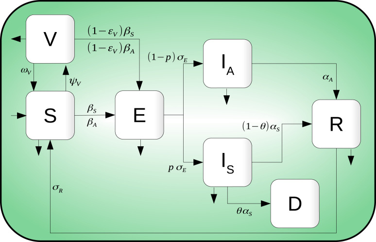
We use an extension of the classical Kermack–McKendrick model. Our formulation considers vaccination and vital dynamics. To this end, for fixed time $t$, we split the total population $N\left(t\right)$, according to the following compartments: susceptible ($S\left(t\right)$), exposed ($E\left(t\right)$), symptomatic infectious ($I_S\left(t\right)$), asymptomatic infectious ($I_A\left(t\right)$), recovered ($R\left(t\right)$), dead ($D\left(t\right)$) and vaccinated ($V\left(t\right)$). Our formulation requires the following hypotheses:

• (H-1)The vaccine is administered to all individuals exempting those with symptoms. Therefore, only individuals in the $S$, $E$, $I_A$ and $R$ classes are candidates for vaccination.
• (H-2)The vaccine only has effects on the susceptible individuals. Thus, susceptible individuals become vaccinated at ${\psi }_V$ rate.
• (H-3)The vaccine only protects against COVID-19.
• (H-4)Individuals get vaccinated only once during the epidemic.
• (H-5)Once an inoculated individual gets vaccine-induced immunity, returns to the $S$ class after a period of time (waning immunity period).
• (H-6)The vaccine is imperfect. A fraction of individuals in $V$ may become infected, with a lower probability than those in the $S$ class.
• (H-7)After a natural immunity period, the recovered population returns to the susceptible class.

Since we will explore disease dynamics that lasts from six months to one year, the model includes vital dynamics. We consider a constant population $(N\left(t\right)=N)$. Thus, we assume that birth and natural death rates are the same and represented by $\mu$. All births lie into the $S$ class and all but class $D$ experience natural death. Class $D$ does not intervene in the transmission dynamics and counts reported deaths.

The infection dynamics are as follows: Susceptible individuals $\left(S\right)$ become infected, but not infectious, when in contact with infectious individuals $I_S$ and $I_A$. Exposed individuals ($E$) remain in their class until they become infectious and move to either $I_S$ or $I_A$. Individuals in class $I_S$ either die by disease complications or recover, whereas individuals in class $I_A$ move to the $R$ class after a some time. Finally, as the vaccine is considered imperfect, individuals in $V$ move to the $E$ class by interacting with infectious individuals $I_S$ and $I_A$ at a lower rate than $S$ individuals. Fig. 1 shows the compartmental model diagram which summarizes hypotheses mentioned above.

Fig. 1.

Compartmental diagram of COVID-19 transmission dynamics which including vaccination dynamics. Here, there are seven different classes: Susceptible $\left(S\right)$, exposed $\left(E\right)$, symptomatic infected $\left(I_S\right)$, asymptomatic infected $\left(I_A\right)$, recovered $\left(R\right)$, death $\left(D\right)$ and vaccinated $\left(V\right)$ individuals.

The model is given by the following ordinary differential equations system

$$S^{\prime }\left(t\right)=\mu \widehat{N}-f_{\lambda }S-(\mu +{\psi }_V)S+{\omega }_{V}V+{\sigma }_{R}R$$$$E^{\prime }\left(t\right)=f_{\lambda }\left(S+(1-{\epsilon }_V)V\right)-(\mu +{\sigma }_E)E$$$$I_S^{\prime }\left(t\right)=p{\sigma }_{E}E-(\mu +{\alpha }_S)I_S$$$$I_A^{\prime }\left(t\right)=(1-p){\sigma }_{E}E-(\mu +{\alpha }_A)I_A$$$$R^{\prime }\left(t\right)=(1-\theta ){\alpha }_S{I}_S+{\alpha }_A{I}_A-(\mu +{\sigma }_R)R$$$$D^{\prime }\left(t\right)=\theta {\alpha }_S{I}_S$$$$V^{\prime }\left(t\right)={\psi }_{V}S-(1-{\epsilon }_V)f_{\lambda }V-(\mu +{\omega }_V)V$$ (1)

where the infection force is defined by

$$f_{\lambda }≔\frac{{\beta }_S{I}_S+{\beta }_A{I}_A}{\widehat{N}}.$$ (2)

Here, $\widehat{N}\left(t\right)=S\left(t\right)+E\left(t\right)+I_S\left(t\right)+I_A\left(t\right)+R\left(t\right)+V\left(t\right)$. For system in Eq. (1) all the variables are taken normalized by the constant total population $N$. Therefore $\widehat{N}+D=1$. Let

$$\Omega =\{(S,E,I_S,I_A,R,D,V)\in {[0,1]}^7:S+E+I_S+I_A+R+D+V=1\}.$$

The dynamics in Eq. (1) is positively-invariant on $\Omega$ (see Appendix B). Additionally, the equations

$$X^{\prime }\left(t\right)={\psi }_V(S+E+I_A+R)$$$$Y_{I_S}^{\prime }\left(t\right)=p{\sigma }_{E}E,$$ (3)

count the cumulative administered vaccines doses until time $t$ as the product $N\times X\left(t\right)$. Also, the cumulative incidence of reported cases is given by $N\times Y_{I_S}\left(t\right)$.

Remark 1

Vaccine is administered to individuals in classes $S$, $E$, $I_A$ and $R$. The amount of given vaccines is quantified by Eq. (3). However, as we assume the vaccine has preventive nature only, there is no change from classes $E$, $I_A$, and $R$ to $V$ due to vaccination.

The parameters of model Eq. (1) are described in Table 1.

Table 1.

Parameters definition of system in Eq. (1).

Parameter	Description
$\mu$	Natural death rate
${\beta }_S\left({\beta }_A\right)$	Symptomatic (Asymptomatic) transmission contact rate
${\psi }_V$	Vaccination rate
${\omega }_V$	Waning rate of vaccine. $1∕{\omega }_V$ is the average time to lose vaccine-induced immunity
${\epsilon }_V$	Vaccine efficacy
${\sigma }_E$	Latency rate. $1∕{\sigma }_E$ is the average latency period
$p$	Exposed individuals’ fraction who become symptomatic infectious
${\alpha }_S$	Transition rate from symptomatic to recover or death. $1∕{\alpha }_S$ is the average output time of symptomatic individuals class
$\theta$	Proportion of symptomatic individuals who die due to the disease
${\alpha }_A$	Recovery rate of asymptomatic individuals. $1∕{\alpha }_A$ is the average time which asymptomatic individuals leave being infectious
${\sigma }_R$	Rate of loss of natural immunity. $1∕{\sigma }_R$ is the natural immunity period

2.1. Calibration of baseline parameters

Multiple COVID-19 studies have shown important differences in transmission contact rates values across countries. For this reason, we establish a set of baseline parameter values for our geographic region of interest: the area constituted by Mexico-City and Mexico-State.

Mexico’s COVID-19 database provides detailed information on reported cases, hospitalized, ambulatory and deaths. Following the ideas of  [15], we consider COVID-19 confirmed deaths data to calibrate both transmission contact rates and exposed individuals proportion who become symptomatic infectious.

To address this problem, we employ a MCMC method. As observation model, we use a negative binomial distribution with mean given by

$$\widehat{D}\left(k\right)=D\left(k\right)-D(k-1)={\int }_{k-1}^k\theta {\alpha }_S{I}_S\left(t\right)dt,$$ (4)

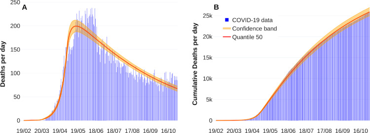
where $\widehat{D}\left(k\right)$ represents the daily deaths incidence at the $k$th day, and $D\left(k\right)$ is the solution of the sixth equation of the system in Eq. (1) without vaccination dynamics at the $k$th day. Fig. 2 shows fitting curves with their respective confidence bands. Estimation process considers data from February 19, 2020, to October 31, 2020. Like other studies [17], [18], it is considered perturbations on both transmission contact rates due to implementing or breaking mitigation measures. For more information about the parameter estimation process, see Appendix A. Table 2 summarizes our parameter calibration.

Fig. 2.

Fitting death curve of the COVID-19 outbreak in Mexico-City and Mexico-State. Panel A shows new reported deaths per day. Panel B represents cumulative deaths per day. Reported deaths data are shown in blue bars from February 19, 2020, to October 31, 2020.

Table 2.

Estimated range for some parameters of system in Eq. (1) without vaccination dynamics.

Parameter	Estimated range	Calibrated
${\beta }_S$	$[\text{0.058 262},\text{0.544 492}]$	0.363282
${\beta }_A$	$[\text{0.101 754},\text{0.441 215}]$	$0.251521$
$p$	$[\text{0.111 348},\text{0.249 985}]$	0.1213

3. Vaccine reproduction number

In this section, we present a formulation for the vaccine reproduction number. Using the definitions of Van den Driessche and Watmough [31], the basic reproductive number for our dynamics without vaccination ($R_0$) and the vaccine reproduction number ($R_V$) are calculated for Eq. (1). Since $R_V$ can be rewritten in terms of $R_0$, this representation will allow us to formulate disease control strategies.

Considering dynamics (1) without vaccination, the basic reproductive number results:

$$R_0=\frac{p{\sigma }_E{\beta }_S}{(\mu +{\sigma }_E)(\mu +{\alpha }_S)}+\frac{(1-p){\sigma }_E{\beta }_A}{(\mu +{\sigma }_E)(\mu +{\alpha }_A)}.$$ (5)

Note that each term of $R_0$ represents the contribution of the symptomatic and asymptomatic infectious, respectively, to the spread of the disease.

On the other hand, the vaccine reproduction number for Eq. (1) is given by (see Appendix B)

$$R_V=R_S+R_A,$$ (6)

where,

$$R_S=\frac{p{\beta }_S{\sigma }_E(\mu +{\omega }_V+(1-{\epsilon }_V){\psi }_V)}{(\mu +{\sigma }_E)(\mu +{\omega }_V+{\psi }_V)(\mu +{\alpha }_S)},\text{and}{R}_A=\frac{(1-p){\beta }_A{\sigma }_E(\mu +{\omega }_V+(1-{\epsilon }_V){\psi }_V)}{(\mu +{\sigma }_E)(\mu +{\omega }_V+{\psi }_V)(\mu +{\alpha }_A)}.$$

Let

$$f_V=\frac{{\epsilon }_V{\psi }_V}{(\mu +{\omega }_V+{\psi }_V)}.$$

This factor encloses parameters corresponding to the vaccine profile (efficacy, waning), and vaccination rate. According to this factor and following the ideas of Alexander et al. [32], the expression (6) can be rewritten as

$$R_V=R_0\left(1-f_V\right).$$ (7)

Note that $\left(1-f_V\right)<1$. Observe that if $R_0<1$, then $R_V<1$. Otherwise, if $R_0>1$ and the following conditions hold

$${\psi }_V>\frac{(R_0-1)(\mu +{\omega }_V)}{({\epsilon }_V-1)R_0+1},$$$${\epsilon }_V>1-\frac{1}{R_0},$$ (8)

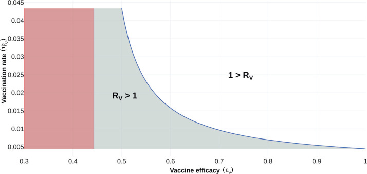
then $R_V$ value is lower than one. Thus, for a waning rate given, there exist an adequate efficacy and vaccination rate to control the disease. However, if the conditions in (8) is not satisfied, it will not be possible to reduce the value of $R_V$ below 1.

To illustrate the aforementioned, Fig. 3 shows the regions where it is possible to reduce the value of $R_V$. In this case, we set all the system parameters as given in Table 3 and fixed ${\omega }_V=1∕180$, leaving ${\epsilon }_V$ and ${\psi }_V$ free.

Fig. 3.

Feasibility region for vaccine reproduction number. The vaccine reproduction number $R_V$ is plotted as a function of vaccine efficacy (${\epsilon }_V$) and vaccination rate (${\psi }_V$). Gray shaded region, corresponds to $R_V>1$. White region, denotes when $R_V<1$. Red region is biologically unfeasible.

Table 3.

Fixed parameters values of system in Eq. (1). The parameters corresponding to vaccination are established in each scenario.

Parameter	Value	95 %CI	Reference/Source
${\alpha }_S$	$\text{0.092 506 9}$	$[\text{0.043 233},\text{0.181 159}]$	[17]
${\alpha }_A$	$\text{0.167 504}$	$[\text{0.086 355},\text{0.198 807}]$	[17]
${\sigma }_E$	$\text{0.196 078}$	$[\text{0.182 815},\text{0.231 481}]$	[33]
${\beta }_S$	$\text{0.363 282}$	a	Calibrated
${\beta }_A$	$\text{0.251 521}$	a	Calibrated
$p$	$\text{0.1213}$	a	Calibrated
${\sigma }_R$	$\text{0.002 739 73}$		Assumed
$\mu$	$\text{0.000 039 138 9}$		Assumed
$\theta$	$\text{0.11}$	b	From data

^aConfidence intervals for parameters ${\beta }_S$, ${\beta }_A$ and $p$ in Table 2 and Appendix A.

^bMedian estimated from Mexico data.

3.1. Baseline vaccination rate

Vaccination policies to reach a given coverage of a certain percentage of the population in a given period is of great importance. In this sense, we refer to this vaccination constant rate as the base vaccination rate, denoted by ${\psi }_{Vbase}$.

Let $W\left(t\right)$ be the normalized unvaccinated population at time $t$. If no individual has been vaccinated at $t=0$, then $W\left(0\right)=1$. Assuming that we vaccinate individuals at a constant rate ${\psi }_{Vbase}$, proportional to the actual population, we have that $W\left(t\right)$ satisfies the equation

$$\dot{W}\left(t\right)=-{\psi }_{Vbase}W\left(t\right)\text{with}W\left(0\right)=1,$$

that is $W\left(t\right)=e^{-{\psi }_{Vbase}t}$. It implies that the number of vaccinated individuals $\left(\widehat{W}\left(t\right)\right)$ at time $t$ is given by $\widehat{W}\left(t\right)=1-e^{-{\psi }_{Vbase}t}$. Therefore, to vaccinate a fraction $z$ of a population in the given time horizon $T$, it follows that ${\psi }_{Vbase}$ satisfies the equation

$$z=1-exp(-{\psi }_{Vbase}T)$$

thus

$${\psi }_{Vbase}=\frac{-ln(1-z)}{T}.$$ (9)

Observe that in the calculation of ${\psi }_{Vbase}$, it is considered all the population to be vaccinated. For our study, vaccination is not applied to symptomatic infectious individuals. Therefore, Eq. (9) represents an approximation of our vaccination coverage $\left(x_{coverage}\right)$ at constant rate.

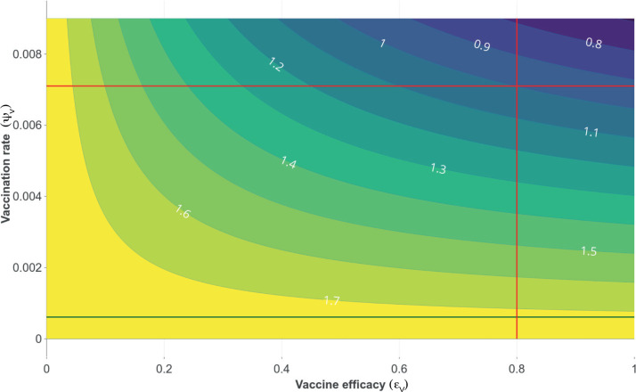
Fig. 4 shows the contour curves for $R_V$ as a function of the vaccine efficacy $\left({\epsilon }_V\right)$ and vaccination rate $\left({\psi }_V\right)$. The green line corresponds to vaccination rate ${\psi }_{Vbase}$ equal to 0.000 611. With this vaccination rate, it is not possible to reduce the value of $R_V$ below one. The intersection of the red lines correspond a vaccine efficacy equals to 0.8 and the corresponding vaccination rate such that $R_V=1$. Note that this vaccination rate values below 0.007 implies $R_V$ greater than 1. Thus, vaccination rate has to be greater than 0.007 in order drives $R_V$ lower to 1. Further, a vaccine efficacy of 50 % or more is required so that, with an adequate vaccination rate, the $R_V$ value can be reduced below one.

Fig. 4.

Contour plot of $R_V$, as a function of vaccine efficacy (${\epsilon }_V$) and vaccination rate (${\psi }_V$) for the case where the average vaccine-induced immunity period is six month. Dark green line represents the value of ${\psi }_{Vbase}=\text{0.000 611}$, corresponding to a coverage $x_{coverage}=\text{0.2}$ and a time horizon $T=\text{365}$ days. Red lines show a scenario in which it is possible to reduce the $R_V$ value below one, considering a vaccine efficacy of 0.8 and a vaccination rate of 0.007.

In the next section, the optimal control theory will be applied to propose optimal vaccination policies that minimize the COVID-19 burden.

4. Optimal vaccination policies

In the remains of this manuscript, we use the following definitions.

Definition 1 Constant Vaccination Policy —

Consider the model in Eqs. (1), (3). A constant vaccination policy (CP) is a policy where the vaccination rate ${\psi }_V$ remains constant for all time $t\in [0,T]$. Thus the number of administered vaccine doses at time $t$ with this CP results

$${\psi }_V\left(S\left(t\right)+E\left(t\right)+I_A\left(t\right)+R\left(t\right)\right)N.$$ (10)

Our main idea is taking ${\psi }_V$ as Eq. (9) and modulating it additively by a time function $u_V\left(t\right)$. We impose that $u_V\left(t\right)\in [-m_1{\psi }_V,m_2{\psi }_V],\forall t\in [0,T]$, $m_1\in [0,1]$, $m_2\in {\mathbb{Q}}^{+}$, then term

$${\psi }_V+u_V\left(t\right),$$ (11)

amplifies or attenuates the constant vaccination rate ${\psi }_V$. If $m_1\in (0,1]$, then control signal $u_V\left(t\right)$ attenuates the vaccination rate ${\psi }_V$. Meanwhile, if $m_2>0$, then control signal $u_V\left(t\right)$ amplifies this vaccination rate.

We modify components equations corresponding to $S$, $V$, $X$ in Eqs. (1), (3) by

$$S^{\prime }\left(t\right)=\mu \widehat{N}-f_{\lambda }S-\left(\mu +({\psi }_V+u_V\left(t\right))\right)S+{\omega }_{V}V+{\sigma }_{R}R$$$$V^{\prime }\left(t\right)=\left({\psi }_V+u_V\left(t\right)\right)S-(1-{\epsilon }_V)f_{\lambda }V-(\mu +{\omega }_V)V$$$$X^{\prime }\left(t\right)=\left({\psi }_V+u_V\left(t\right)\right)(S+E+I_A+R).$$ (12)

Then our controlled dynamics reads

$$\begin{array}{cc}\hfill S^{\prime }\left(t\right)& =\mu \widehat{N}-f_{\lambda }S-(\mu +{\psi }_V+u_V\left(t\right))S+{\omega }_{V}V+{\sigma }_{R}R\hfill \\ \hfill E^{\prime }\left(t\right)& =f_{\lambda }(S+(1-{\epsilon }_V)V)-(\mu +{\sigma }_E)E\hfill \\ \hfill I_S^{\prime }\left(t\right)& =p{\sigma }_{E}E-(\mu +{\alpha }_S)I_S\hfill \\ \hfill I_A^{\prime }\left(t\right)& =(1-p){\sigma }_{E}E-(\mu +{\alpha }_A)I_A\hfill \\ \hfill R^{\prime }\left(t\right)& =(1-\theta ){\alpha }_S{I}_S+{\alpha }_A{I}_A-(\mu +{\sigma }_R)R\hfill \\ \hfill D^{\prime }\left(t\right)& =\theta {\alpha }_S{I}_S\hfill \\ \hfill V^{\prime }\left(t\right)& =({\psi }_V+u_V\left(t\right))S-\left((1-{\epsilon }_V)f_{\lambda }V+\mu +{\omega }_V\right)V\hfill \\ \hfill X^{\prime }\left(t\right)& =({\psi }_V+u_V\left(t\right))(S+E+I_A+R)\hfill \\ \hfill Y_{I_S}^{\prime }\left(t\right)& =p{\sigma }_{E}E,\hfill \\ \hfill \\ \hfill S\left(0\right)& =S_0,E\left(0\right)=E_0,I_S\left(0\right)=I_{S_0},\hfill \\ \hfill I_A\left(0\right)& =I_{A_0},R\left(0\right)=R_0,D\left(0\right)=D_0,\hfill \\ \hfill V\left(0\right)& =0,X\left(0\right)=0,Y_S\left(0\right)=Y_{S_0}\hfill \\ \hfill \widehat{N}\left(t\right)& =S+E+I_S+I_A+R+V.\hfill \end{array}$$ (13)

Formally we define a controlled vaccination policy as follows.

Definition 2 Controlled Vaccination Policy —

Conforming the model in Eq. (13) we say that

$${\psi }_V+u_V\left(t\right),t\in [0,T],$$

is a controlled vaccination policy (CVP). Then,

$$({\psi }_V+u_V\left(t\right))\left(S\left(t\right)+E\left(t\right)+I_A\left(t\right)+R\left(t\right)\right)N,$$

denote the number of doses at time $t$ according to the modulated vaccination rate $({\psi }_V+u_V\left(t\right))$.

We aim to obtain time-control functions $u_V\left(\cdot \right)$ that hold natural modeling constraints—as a fixed bound for hospitalized prevalence and coverage at the final time—and optimize a conveniently cost functional. To this end, we have to assure our optimal controlled model solution, so we consider the functional space

$$\mathcal{U}[0,T]≔\left\{u_V:[0,T]\to \mathbb{R},\right)$$$$\text{ such that }{u}_V\left(\cdot \right)\text{ bounded and}$$$$\left(\text{ piecewise continuous}\right\}.$$ (14)

Let $x\left(t\right)≔{(S,E,I_S,I_A,R,D,V,X,Y_{I_S})}^{\top }\left(t\right)$ and control signal $u_V\left(\cdot \right)\in \mathcal{U}[0,T]$. Following the guidelines of WHO-SAGE modeling questions [3], we quantify the burden of COVID-19, according to the DALY indicator. Adapting DALY’s definition reported in [34], we optimize the number of years of life lost with a controlled vaccination policy. Our formulation calculates a minimum of the penalization functional

$$J\left(u_V\right)=a_D(D\left(T\right)-D\left(0\right))+a_S(Y_{I_S}\left(T\right)-Y_{I_S}\left(0\right)).$$ (15)

Here, $a_S$ and $a_D$ are parameters related to the definition of the Years of Life Lost (YLL) due to premature mortality and the Years Lost due to Disability (YLD). We estimate $a_D$ as the average remaining life expectancy at the age of death, and according to the union of Mexico-City and Mexico-State data, we set $a_D=\text{7.5}\text{years}$. Parameter $a_S$ is the product of a disability weight (DW) and the average duration of cases until remission or death in years, that is, $a_S=DW\times {\alpha }_S^{-1}$. Here we postulate the disability weight as the arithmetic average of disability weight regarding comorbidities reported in [35]. Our simulations employ $a_S=\text{0.008 418 473}\text{years}$. Thus, functional $J$ penalizes the pandemic burden—in Years of Life Lost—due to mortality or disability.

To describe vaccination coverage, we ask the terminal condition

$$\phi \left(x\left(T\right)\right)=X\left(T\right),$$$$S\left(T\right)+E\left(T\right)+I_S\left(T\right)+I_A\left(T\right)+R\left(T\right)+V\left(T\right)+D\left(T\right)=1,$$$$X\left(T\right)=x_{coverage},$$$$x_{coverage}\in \left\{\text{Low(0.2)},\text{Mid(0.5)}\right\}.$$ (16)

That is, given the time horizon $T$, we set the vaccination coverage to 20 % or 50 % of the total population, and the rest of final states free. Likewise, we impose the path constraint

$$\Phi (x,t)≔\kappa I_S\left(t\right)\le B,\forall t\in [0,T],$$ (17)

to ensure that critical symptomatic cases will not overload healthcare services. Here $\kappa$ denotes hospitalization rate, and $B$ is the load capacity of the health system.

Definition 3 Admissible Control Vaccination Policy —

Let $(x\left(\cdot \right),u_V\left(\cdot \right))$ be a pair satisfying the ODE (13). Consider $\mathcal{U}[0,T]$ as in (14). If

• (AC-1) $u_V\left(\cdot \right)\in \mathcal{U}[0,T]$
• (AC-2)$u\left(t\right)\in [-m_1{\psi }_V,m_2{\lambda }_V],\forall t\in [0,T]$,  $m_i\in \mathbb{Q}$
• (AC-3) $x\left(T\right)={(\cdot ,\cdot ,\cdot ,\cdot ,\cdot ,\cdot ,\cdot ,x_{coverage},\cdot )}^{\top }$
• (AC-4) $\kappa I_S\left(t\right)\le B,\forall t\in [0,T]$

holds, then the CVP ${\psi }_V+u_V\left(\cdot \right)$ is admissible.

In other words, an admissible vaccination policy (AVP) is a CVP that satisfies the coverage and hospitalization constraints imposed on model (13). Furhter, if an AVP optimizes functional cost (15), then this AVP is an optimal vaccination policy (OVP). Formally we have the following definition.

Definition 4 Optimal Vaccination Policy —

Let $(x\left(\cdot \right),u_V\left(\cdot \right))$ a pair that satisfies the ODE (13) such that (AC-1)–(AC-4) of Definition 3 holds. Let cost functional $J$ as in (15). If

$$J\left(u_V\right)=\underset{u\in {\mathcal{U}}^{\star }}{min}J\left(u\right),$$$${\mathcal{U}}^{\star }:=\mathcal{U}[0,T]\cap \{u\left(\cdot \right):\text{(ADC-1)–(ADC-4) holds}\},$$ (18)

then ${\psi }_V+u_V\left(\cdot \right)$ is an optimal vaccination policy.

Remark 2

Optimal vaccination amplifies or attenuates the estimated baseline ${\psi }_V$ in an interval $[{\psi }_V^{min},{\psi }_V^{max}]$ to optimize functional $J\left(\cdot \right)$—minimizing symptomatic incidence and death reported cases in DALYs and satisfying hospitalization occupancy and coverage constraints.

We aim to minimize the cost functional (15)—over an appropriated space—subject to the dynamics in Eq. (13), coverage related to the boundary condition (16), and path constraints (17). We call this kind of policies as optimal vaccination policies (OVP). That is, we seek vaccination policies that solve the following problem.

Optimal Control Problem (OCP): Find the optimal vaccination rate $({\psi }_V+u_V^{\ast })$ such that,

$$\begin{array}{cc}\hfill J\left(u_V^{\ast }\right)& =\underset{u_V\in {\mathcal{U}}^{\star }}{min}J\left(u_V\right)\hfill \\ \hfill J\left(u_V\right)& ≔a_D(D\left(T\right)-D\left(0\right))+a_S(Y_{I_S}\left(T\right)-Y_{I_S}\left(0\right))\hfill \\ \hfill \text{subject to}& \hfill \\ \hfill f_{\lambda }& ≔\frac{{\beta }_S{I}_S+{\beta }_A{I}_A}{\widehat{N}}\hfill \\ \hfill S^{\prime }\left(t\right)& =\mu \widehat{N}-f_{\lambda }S-(\mu +{\psi }_V+u_V\left(t\right))S+{\omega }_{V}V+{\sigma }_{R}R\hfill \\ \hfill E^{\prime }\left(t\right)& =f_{\lambda }(S+(1-{\epsilon }_V)V)-(\mu +{\sigma }_E)E\hfill \\ \hfill I_S^{\prime }\left(t\right)& =p{\sigma }_{E}E-(\mu +{\alpha }_S)I_S\hfill \\ \hfill I_A^{\prime }\left(t\right)& =(1-p){\sigma }_{E}E-(\mu +{\alpha }_A)I_A\hfill \\ \hfill R^{\prime }\left(t\right)& =(1-\theta ){\alpha }_S{I}_S+{\alpha }_A{I}_A-(\mu +{\sigma }_R)R\hfill \\ \hfill D^{\prime }\left(t\right)& =\theta {\alpha }_S{I}_S\hfill \\ \hfill V^{\prime }\left(t\right)& =({\psi }_V+u_V\left(t\right))S-\left((1-{\epsilon }_V)f_{\lambda }V+\mu +{\omega }_V\right)V\hfill \\ \hfill X^{\prime }\left(t\right)& =({\psi }_V+u_V\left(t\right))(S+E+I_A+R)\hfill \\ \hfill Y_{I_S}^{\prime }\left(t\right)& =p{\sigma }_{E}E,\hfill \\ \hfill \\ \hfill S\left(0\right)& =S_0,E\left(0\right)=E_0,I_S\left(0\right)=I_{S_0},\hfill \\ \hfill I_A\left(0\right)& =I_{A_0},R\left(0\right)=R_0,D\left(0\right)=D_0,\hfill \\ \hfill V\left(0\right)& =0,X\left(0\right)=0,Y_S\left(0\right)=Y_{S_0},X\left(T\right)=x_{coverage},\hfill \\ \hfill u_V\left(\cdot \right)& \in [u_{min},u^{max}],\hfill \\ \hfill \kappa I_S\left(t\right)& \le B,\forall t\in [0,T],\hfill \\ \hfill \widehat{N}\left(t\right)& =S+E+I_S+I_A+R+V.\hfill \end{array}$$ (19)

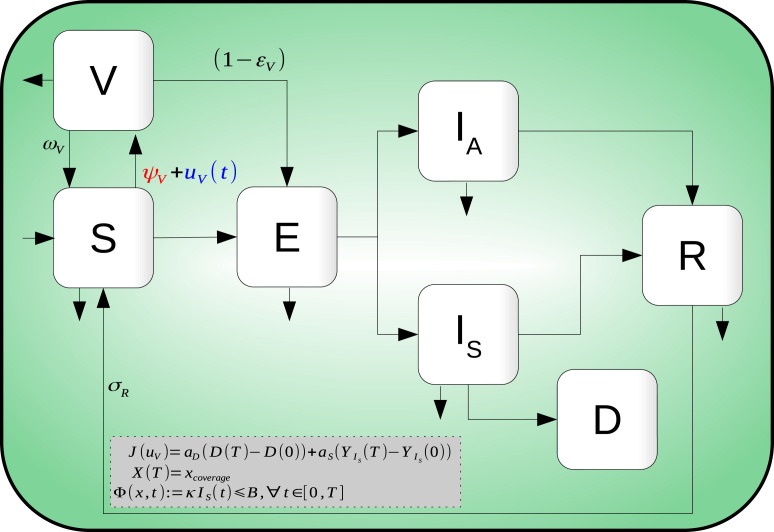
Fig. 5 illustrates the main ideas of the above discussion. Table 4 enclose parameter information of the functional cost and constraints.

Fig. 5.

Compartmental diagram of COVID-19 transmission dynamics that includes optimal vaccination dynamics (19), penalization and a path constraint.

Table 4.

Parameters regarding the constraints conditions and cost functional of the OCP (19).

Symbol	Description	Value	Ref
$a_D$	Penalization weight due to premature mortality (YLL) and estimated from Mexico-City an Mexico-State data	$\text{7.5}\text{years}$	[34], [37]
$a_S$	Penalization weight due to disability (YLD)	$\text{0.008 418 473}\text{years}$	[35]
$x_{coverage}$	Covering constraint at time horizon $T$		[3]
$\kappa$	Hospitalization rate	0.05	Estimated
$B$	Health service capacity in number of beds	9500	Estimated

Existence of solution to our (OCP) in Eq. (19) drops in the theory developed by Francis Clark [see e.g. 36, Thm. 23.11]. Since we aim to simulate hypothetical scenarios, we omit here a rigorous proof. Instead, we refer interested readers to [23] and the reference therein.

5. Numerical experiments

5.1. Methodology

We apply the so-called transcript method to solve our (OCP). This method transforms the underlying problem of optimizing functional governed by a differential equation into a finite-dimensional optimization problem with restrictions. To fix ideas, let $x$, $u$ respectively denote state and control, and consider the optimal control problem

$$minJ(x\left(\cdot \right),u\left(\cdot \right))=g_0(T,x\left(T\right))\text{Functional cost}$$

$$\dot{x}=f(t,x\left(t\right),u\left(t\right)),\forall t\in [0,T],\text{Dynamics}$$

$$u\left(t\right)\in \mathcal{U}[0,T]\text{for a.e. }t\in [0,T]\text{Admissible controls}$$

$$g(x\left(t\right),u\left(t\right))\le 0\text{Path constrain}$$

$$\Phi (x\left(0\right),x\left(T\right))=0\text{Boundary conditions}.$$

Then, transcription methods transform this infinite-dimensional optimization problem into a finite dimension problem (NLP) via discretization of dynamics, state, and control. For example, if we employ the Euler method with a discretization of $N$ constant steps with size $h$, then we can solve

$$min{g}_0(t_N,x_N)$$$$x_{i+1}=x_i+hf(x_i,u_i),i=0,\dots ,N-1$$$$u_i\in \mathcal{U},i=0,\dots ,N$$$$g(x_i,u_i)\le 0,i=0,\dots ,N$$$$\Phi (x_0,x_N)=0,i=0,\dots ,N,$$ (20)

where $x_i\approx x\left(t_i\right)$, $u_i\approx u\left(t_i\right)$ in the grid

$$\left\{t_0=0,t_i=ih(i=1,\dots ,N-1),t_N=T\right\}.$$

Let $Y=\{x_0,\dots ,x_N,u_0,\dots u_N\}$. Thus Eq. (20) defines a nonlinear programming problem on the discretized state and control variables of the form

$$minF\left(Y\right)$$$$\text{such that}$$$$LB\le C\left(Y\right)\le UB.$$ (21)

The numerical analysis and design of transcript methods is a well-established and active research numerical field. There is a vast literature about robust methods, and recently, implementations have been developed in vogue languages like Julia  [38], Python [39], and others.

Our simulations rely on the Bocop package  [40] to solve our OCP. Bocop is part of the development of the INRIA-Saclay initiative for open source optimal control toolbox and supported by the team Commands. BOCOP solves the NLP problem in Eq. (21) by the well-known software Ipopt and using sparse exact derivatives computed by ADOL-C.

We provide in [41] a GitHub repository with all regarding Bocop sources.

5.2. Hypothetical scenarios

Following the guidelines reported by the WHO Strategic Advisory Group of Experts (SAGE) on Immunization Working Group on COVID-19 Vaccines modeling questions presented in [3]. We simulate scenarios to illustrate vaccination policies’ response with a preventive vaccine. We aim to contrast the impact on the burden of COVID-19, according to

• (SCN-1)

  Optimal versus constant vaccination policies

• (SCN-2)

  Vaccine efficacy

• (SCN-3)

  Induced vaccine immunity

• (SCN-4)

  Natural immunity

We consider vaccine efficacies and doses compatible with the firms CansinoBio and Johnson & Johnson [42]. Although other firms such as Pfizer-BioNTech, Moderna, Astra-Zeneca, Gamaleya Research Institute, Sinovac Biotech, among others, require two doses [10], [43], [44], as a first approximation, our model simulates their total efficacy in a single dose. Further, since reinfection and vaccine-induced immunity parameters remain unavailable, we see it pertinent to explore the effect of plausible settings.

Remark 3

Optimal vaccination policy implies that number of doses per unit time described by

$$({\psi }_V+u_V\left(t\right))(S\left(t\right)+E\left(t\right)+I_A\left(t\right)+R\left(t\right))N$$

mitigates the outbreak in optimal form, where optimal is defined in terms of function $J\left(\cdot \right)$ (see Eq. (15)), that is minimizing years of life lost in DALYs. Counterfactual scenarios implies ${\psi }_V+u_V\left(t\right)=0,\forall t\in [0,T]$. Constant vaccination policy means $u_V\left(\cdot \right)=0$.

Remark 4

We assume positive prevalence of all epidemiological classes according to the following hypothesis:

• (IC)-1The implemented initial conditions for our numerical experiments are hypothetical and do not reflect the actual data reported by Mexico-City and Mexico-State health authorities. The initial conditions are taken such that an outbreak is on its growth phase.
• (IC)-2We suppose that around of 30 % of the population is under Lockdown and is enclosed along with recovered class $R$. That is, $R\left(0\right)$ encircle mainly children, senior, home office, people with low mobility and COVID-19 recovered individuals.
• (IC)-3Our numerical results are of qualitative nature and not necessarily sustain forecasting or follows the actual profile of the underlying COVID-19 pandemic data.

Table 5 encloses a brief description and parameter values regarding each scenario. The reader can also access the web Chart Studio Graph of each figure regarding data and plotly [45] visual representation.

Table 5.

Setup parameters for counterfactual and response scenarios. See Table 2 for the rest of parameters.

Simulation scene	Description	Set-up  $(x_{coverage},T,{\epsilon }_V,{\omega }_V^{-1},{\sigma }_R^{-1})$
(SCN-1)	Likening between optimal and constant vaccination policies.	(20  % , 180  days , 70  % , 730  days , lifelong )
(SCN-2)	Vaccine efficacy blow	(50  % , 365  days , $\left\{\text{50}\text{\%},\text{70}\text{\%},\text{90}\text{\%}\right\}$, 730  days , 180  days )
(SCN-3)	Vaccine-induced immunity period	(50  % , 365  days , 90  % , $\left\{\text{180}\text{days},\text{365}\text{days},\text{730}\text{days}\right\}$, 365  days )
(SCN-4)	Natural immunity period	(50  % , 365  days , 90  % , 730  days , $\left\{\text{90}\text{days},\text{180}\text{days},\text{365}\text{days}\right\}$)

To perform the simulations corresponding to the scenarios presented in Table 5, we fix the parameter values as in Table 6.

Table 6.

Fixed parameters values of system in Eq. (19).

Parameters values
	(SCN-1)–(SCN4)
${\beta }_S$, ${\beta }_A$, ${\alpha }_S$, ${\alpha }_A$, ${\sigma }_E$, $\mu$, $\theta$, $p$	Table 2
$a_D$, $a_S$, $\kappa$, $B$	Table 4
	(SCN-1)	(SCN-2)–(SCN-4)
${\psi }_V$	0.001 239 69	0.001 899 03
$u_{min}$	−0.5${\psi }_V$	−0.5${\psi }_V$
$u_{max}$	5${\psi }_V$	2.5${\psi }_V$

Optimal versus constant vaccination policies: (SCN-1)

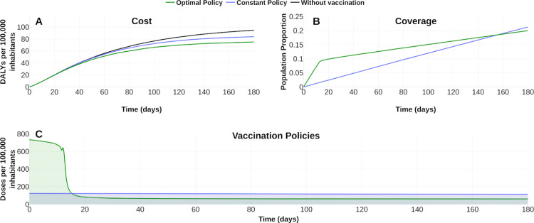
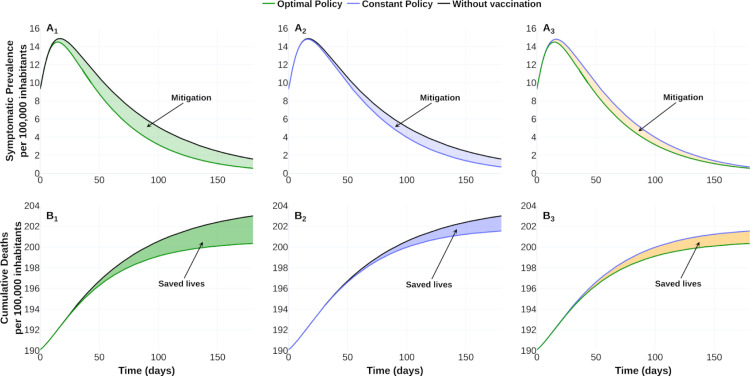
To fix ideas, we display in Fig. 6, Fig. 7 the counterfactual scenario regarding no intervention, constant vaccination policy (CP), and optimal vaccination policy (OVP) with a vaccine profile of efficacy ${\epsilon }_V=\text{70}\text{\%}$, vaccine-induced immunity ${\omega }_V^{-1}=\text{730}\text{days}$ and a campaign for 20 % of coverage at 180 days. Fig. 6 suggests that the OVP improves CP response and counterfactual scenario given by the disease burden quantified in DALYs. Fig. 7 confirms this improvement by comparing disease dynamics with and without vaccination. We observe CP and OVP reduce the symptomatic prevalence and the cumulative deaths. Note that despite OVP requires less doses amount than CP at the time horizon (see Fig. 6B), the OVP performs better than CP (see Fig. 7).

Fig. 6.

Effect of the vaccination policy on the burden COVID-19 for a 20% coverage at time horizon of half year. (A) Vaccination policies’ response regarding constant (${\psi }_V$) and optimal (${\psi }_V+u_V\left(t\right)$) vaccination rates in the burden of COVID-19 quantified in DALYs. (B) Evolution of the vaccination covering according to each policy. (C) Vaccination schedule for each vaccination policy. Blue line corresponds to policies with constant vaccination rate 0.001 239 69. Green line corresponds to optimal vaccination policy. For counterfactual reference (panel A), black line represents the burden of COVID-19 without vaccination. See https://plotly.com/ MAAZ/366/ for plotly visualization and data.

Fig. 7.

Effect of the vaccination policy on outbreak evolution. Optimal policy versus no vaccination (first column), constant policy versus no vaccination (second column) and optimal versus constant policy (third column). Upper row shows the symptomatic prevalence per 100 000 inhabitants. Lower row illustrates cumulative deaths (per 100 000 inhabitants). The shaded area represents the improvement of one policy over its corresponding. Data and web visualization in https://plotly.com/ MAAZ/474/.

Vaccine efficacy (SCN-2)

In February 2021, multiple vaccines have been rolled out to prevent COVID-19 disease. Table 7 summarizes some of these vaccine efficacies. To encompass these scenarios we focus on the 50 %, 70 % and 90 % vaccine efficacies.

Table 7.

Vaccine efficacy of some of the approved developments for emergency use.

Developer	Vaccine name	Vaccine efficacy %, (95% CI)	Reference
Pfizer-BioNTech	BNT162b2	95(90.3 –97.6 )	[46]
Gamaleya Institute	Sputnik V	91.6(85.6 –95.2 )	[44]
Oxford University-AztraZeneca	AZD1222	74.6(41.6 -88.9 )	[10]
Johnson & Johnsona	Ad26.COV2.S	57 %, 66  % or 72  %	[4]
Sinovac Biotecha	CoronaVac	50.4 %	[42]

^aNo available information about the confidence intervals.

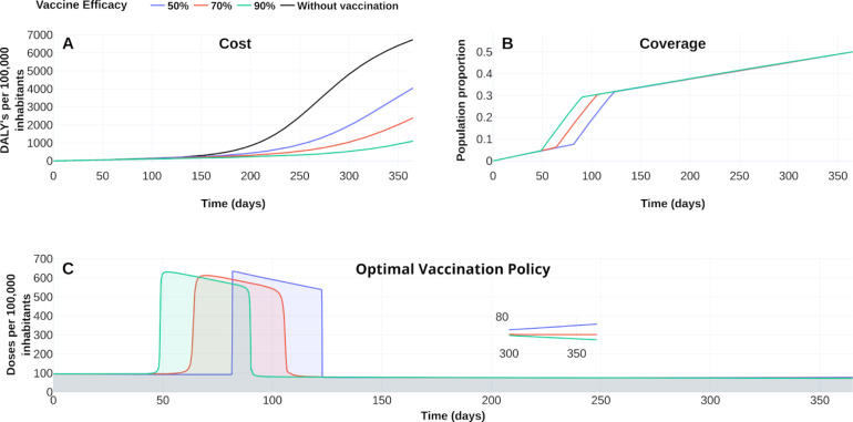
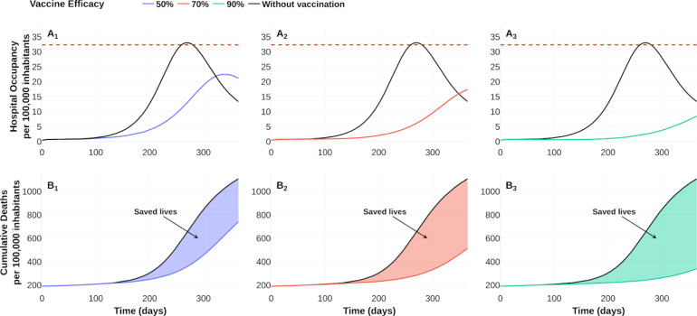
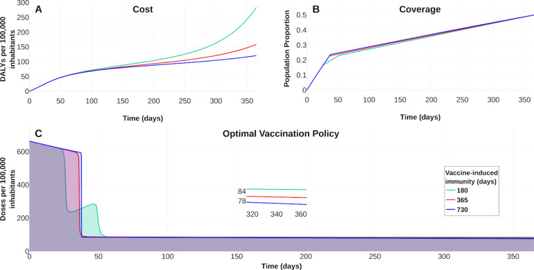
Fig. 8, Fig. 9 display the optimal vaccination policy’s response according to the vaccine efficacies above mentioned. Fig. 8A displays COVID-19 burden in DALYs for the different vaccine efficacies and without vaccination dynamics. Clearly, the higher the vaccine efficacy, the lower the DALYs become.

Fig. 8.

The response of COVID-19 burden on vaccine efficacy. (A) COVID-19 burden response quantified in DALYs per 100 000 inhabitants to vaccines with efficacy of 50 % (blue), 70 % (red) and 90 %(green). (B) Coverage evolution to reach 50 % of the total population vaccinated. (C) Optimal vaccination doses schedule according to the different efficacies. See https://plotly.com/ MAAZ/358/ for visualization and data.

Fig. 9.

Effect of vaccine-efficacy on hospital occupancy and on the number of saved lives compared to no vaccination dynamics. Vaccine-efficacy of 50 % (blue), 70 % (red) and 90 % (green). Dotted red line represents 90 % of hospital beds per 100 000 inhabitants. See https://plotly.com/ MAAZ/470/ for data and visualization.

Figs. 8B–C also illustrate the effect of vaccine-efficacies on coverage and optimal vaccination policy, respectively. We observe that vaccine efficacy influences the design of an optimal policy. For this scenario the higher vaccine efficacy, the earlier is its massive implementation. According to 50 % coverage at a time horizon of 1 year, Fig. 9 displays an improvement from 1.5 to 3 times regarding the counterfactual scenario for the cumulative deaths at time horizon. Also, there is a notorious improvement in the hospital occupancy. For the no vaccination dynamics, the hospital occupancy exceeds the 90% of beds (dashed red line in Fig. 9). In contrast, for the considered controlled dynamics, the higher hospital occupancy lowers to about 63% of beds (see Fig. 9A${}_1$).

Vaccine-induced immunity (SCN-3)

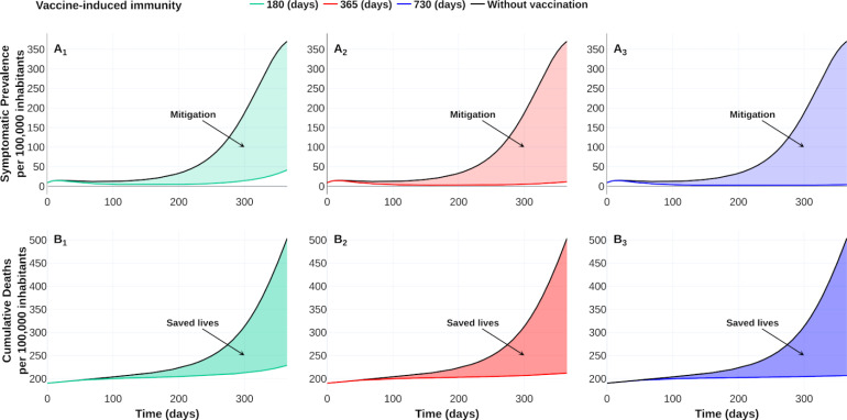
Vaccine response and its induced immunity are strongly related on the mitigation prevalence. However, vaccine-induced immunity period remains poorly understood [8]. Here, we contrast three vaccines with different induced-immunity. Let denote by $va{x}_1$, $va{x}_2$, $va{x}_3$ vaccines with an induced-immunity period of a half, one, and two years, respectively, and common efficacy of 90 %. Consider a vaccine campaign of time horizon of one year and 50 % coverage. Taking the same initial conditions, and parameters values, as in Table 2, we explore the vaccines’ consequences versus the counterfactual scenario with $R_0=\text{1.794 93}$. Vaccine reproduction number, at the initial time of the optimal policy, for each vaccine results in $R_V^{\left[va{x}_1\right]}=\text{0.917 813 4}$, $R_V^{\left[va{x}_2\right]}=\text{0.655 909 4}$, $R_V^{\left[va{x}_3\right]}=\text{0.462 048 9}$ for vaccine-induced immunity periods of a half, one, and two years, respectively. We display in Fig. 10 the response of the vaccines $va{x}_1$, $va{x}_2$ and $va{x}_3$. Since optimal vaccination policies are similar, Fig. 10C suggests that the vaccine-induced immunity rate is not determinant in the vaccination schedule design. Fig. 11 shows a wide reduction of prevalence and cumulative deaths concerning the uncontrolled outbreak. This reduction is consistent with the vaccine reproductive number values corresponding to each vaccine-induced immunity. Thus, vaccine reproductive number values highlight the importance of having an adequate vaccine profile and adequate vaccine schedule to control the epidemic outbreak.

Fig. 10.

Vaccine-induced immunity effect on the COVID-19 burden. (A) Effect on the burden of COVID-19 quantified in DALYs per 100 000 inhabitants due to vaccine-induced immunity of 180 days (green), 365 days (red) and 730 days (blue). (B) Coverage evolution to reach 50 % of the total population vaccinated. (C) Optimal vaccination doses schedule according to the different vaccine-induced immunity periods. Visualization and data in https://plotly.com/ MAAZ/407/.

Fig. 11.

Effect of vaccine-induced immunity on mitigation and saved lives of COVID-19 outbreak. Upper row shows the improvement of optimal vaccination policy over no vaccination dynamics on the symptomatic prevalence per 100 000 inhabitants. Lower row shows a comparison of the saved lives (per 100 000 inhabitants) between optimal policies and no vaccination dynamics. Optimal policy with vaccine-induced immunity of a half year versus no vaccination dynamics (first column), optimal policy with vaccine-induced immunity of a year versus no vaccination dynamics (second column), and optimal policy with vaccine-induced immunity of two years versus no vaccination dynamics (third column). See https://plotly.com/ MAAZ/465/ for data and visualization.

Natural immunity hypothesis (SCN-4)

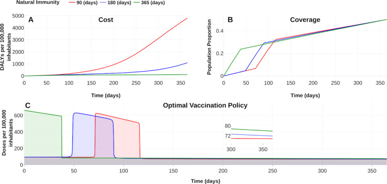
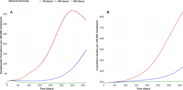
“Reinfections raise questions about long-term immunity to COVID-19 and the prospects for a vaccine”, reported Heidi Ledford in [47]. Following this line, we display in Fig. 12, Fig. 13 the vaccine’s response with 90 % efficacy and contrasting with natural immunity periods of 90 days, 180 days, and 365 days. Here, the adjective “natural” denotes the immunity that an individual develops after recovering from a previous bout of COVID-19 without vaccination. Fig. 12A shows that, if natural immunity lasts one year, then burden of COVID-19 falls until around 120 DALYs. We confirm this fall in the reduction of the symptomatic prevalence cases and cumulative deaths, as displayed in Fig. 13. When natural immunity is 365 days, the benefit in reducing symptomatic prevalence concerning a natural immunity of 90 days is at least 100 times. The number of deaths with a natural immunity of 90 days reaches 845 cases per 100 000 inhabitants, in contrast, to 206 cases when natural immunity is 365 days. Thus, this scenario suggests that natural immunity plays an essential role in controlling the outbreak, consistent with the conclusions reported in [8].

Fig. 12.

Effect of natural immunity on the burden of COVID-19. (A) Effect on the burden of COVID-19 quantified in DALYs per 100,000 inhabitants due to natural immunity of 90 days (red), 180 days (blue) and 365 days (green). (B) Coverage evolution to reach 50 % of the total population vaccinated. (C) Optimal vaccination doses schedule according to the different natural immunities. https://plotly.com/ MAAZ/402/.

Fig. 13.

Effect of natural immunity on COVID-19 outbreak. (A) Effect of natural immunity over the symptomatic prevalence per 100 000 inhabitants. (B) Improvement of natural immunity over the cumulative deaths per 100 000 inhabitants. Plotly visualization and data in https://plotly.com/ MAAZ/451/.

6. Discussion

In February 2021, at least four vaccination developments support the primary pharmaceutical measure to recover life’s style before the pandemic. Although the leading pharmaceutics firms report high vaccine efficacy, its implementation implies new challenges as its distribution, stocks, politics, logistic, among others, emerge. A fair distribution and application strategy is imperative to manage the available resources. Despite that vaccine-immunization response remains under study, vaccination campaigns recently started. Thus evaluating the impact of different vaccine profiles and natural immune responses would be crucial to calibrate vaccination policies. Further, since the vaccine doses are scarce at the beginning of the COVID-19 vaccination campaigns optimize their administration subject to its availability, minimizing deaths and preserving health systems is mandatory.

We aim to compare different vaccine profiles in computing optimal vaccination policies for COVID-19 and evaluate the impact of hypothetical reinfection and immunization responses. Our simulations suggest that an optimal strategy design is influenced by vaccine profile and natural immunity period. Likewise, we observe that natural and vaccine-induced immunity would play an essential role in reducing COVID-19 disease mortality and prevalence levels. Poland et al. [48] stress that understanding immune responses to SARS-CoV-2 are crucial to developing vaccines. Our simulation faces different vaccine-induced and natural immunization profiles, allowing the study of these variables’ effects and developing optimal dose administration schedules. Further, our optimal solution satisfies modeling constraints to obtain the desired vaccination coverage and avoid health system overload. We optimized vaccination strategies by minimizing the COVID-19 burden quantified in DALYs.

Note that the elderly population has been the most affected in terms of deaths due to the disease. Thus, the average remaining expectancy of lives could be explained by this population. It is well know that stratification becomes important when vaccination strategies prioritize risk groups to reduce burden. Although our model lacks an age-stratified structure, these results would apply to situations where the population has homogeneous characteristics. This kind of population’s designs arises, for example, in places like factories, offices, or even schools. The question “who vaccinate first¿‘ has been faced as an optimal allocation problem in [25], [26], [27]. Our optimal solutions have a complementary objective—while we answer when and how to administrate vaccine doses, the mentioned references answer who vaccinate first.

In [30] the authors answered when to vaccinate optimally. They used a signal that switches between not vaccination and immunization of all susceptible individuals. Since the vaccine is scarce, this control signal would be unrealistic in some situations. Our results improve this strategy by modulating a base vaccination rate in a more realistic bound. Further, we consider more detailed dynamics: our model includes exposed and dead classes and differences between symptomatic infectious kinds.

We relate vaccination rate with the available vaccine stock and health system response—limited by logistics, management, politics, and other issues related to each vaccine development. So, our contribution can help decision-makers to design vaccination schedules of homogeneous populations.

When writing this article, the vaccine-induced immunity period and SARS-CoV-2 transmission capacity from a vaccinated individual remain unexplained [48]. The conclusive answer inevitably will drive the development of COVID-19 vaccines and their policies. Experts estimate that around 7 800 billion immunization doses are required to reach herd immunity. This number, with the approved developments, is far away to accomplish in one year. However, we expect that more vaccines finish their third trial phase and also get approval. Thus, vaccination policies also have to contemplate two o more vaccine profiles, perhaps with different efficacy o number of recommended doses.

These issues also have to balance the health services and other resources optimally.

7. Conclusions

The absence of proven highly effective treatments against COVID-19 has led the world’s population to pin their hopes on vaccines. However, due to the limited stock of vaccines, the question arises as to which is the best vaccination strategy. Thus, different researchers have sought to answer this question from different perspectives. In the present work, we address this question through an optimal control approach. Our results show the importance of how and when to vaccinate on reducing disease levels.

The scarce information regarding immunity periods and the wide efficacy range of the approved vaccines highlights the importance of exploring scenarios with different vaccination profiles. This study observes the importance of knowing the vaccine profile and the natural immunity period to design an optimal vaccination strategy. For example, SCN-2 and SCN-4 scenarios show that an optimal vaccination strategy does not necessarily imply massive vaccination at the beginning. For the former, the vaccine efficacy level (Fig. 8) is a responsible factor to determine the beginning time of the massive vaccination strategy whereas for the latter is the natural immunity period (Fig. 12).

Nowadays, several countries have problems with vaccine stocks. In addition, the uncertainty regarding induced immunity and natural immunity has forced governments to implement vaccination programs aimed at specific populations such as medical personnel, elderly population, teachers, etc., with similar characteristics to each other. Our work can be useful in decision-making for the design of vaccination programs targeted to this populations types, since it considers stock constraints and explores different vaccination profiles and natural immunity to design optimal vaccination strategies.

At the date of writing this manuscript, several questions about vaccines and COVID-19 disease have not been addressed thoroughly. How often shall we need to get vaccinated, once in a lifetime or yearly? Do all the vaccines’ acquired immunity last equally? If the latter is false, what are the consequences of implementing campaigns with different vaccines? Would the vaccines be produced on a much larger scale than now? If the latter is true, when, how, and to whom should vaccines be given to obtaining greater reductions on incidence levels? What effect will the new COVID-19 variants have on the vaccines developed? Would the vaccines’ effectiveness significantly decrease? If the latter is true, then would be necessary more doses for each vaccine? All these questions will eventually become daily concerns in society as time passes by. Thus, optimal vaccination strategies take more relevance to address some of these questions.

Motivated by the above, as future work, we analyze extending our study when considering a stratified population problem and more than one vaccine with different efficacies and number of doses. We aim to answer some of the previously raised questions over non-homogeneous populations.

CRediT authorship contribution statement

Manuel Adrian Acuña-Zegarra: Conceptualization, Methodology, Software, Validation, Formal analysis, Investigation, Resources, Visualization, Project administration, Writing - original draft, Writing - review & editing. Saúl Díaz-Infante: Conceptualization, Methodology, Software, Validation, Formal analysis, Investigation, Data curation, Visualization, Supervision, Writing - original draft, Writing - review & editing. David Baca-Carrasco: Conceptualization, Methodology, Formal analysis, Writing - original draft, Writing - review & editing. Daniel Olmos-Liceaga: Conceptualization, Methodology, Formal analysis, Writing - original draft, Writing - review & editing.

Declaration of Competing Interest

The authors declare that they have no known competing financial interests or personal relationships that could have appeared to influence the work reported in this paper.

Appendix A. Parameter estimation

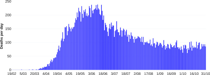
Parameter estimation is based on reported data of deaths by COVID-19 of Mexico-City and Mexico-State. We considered the first 256 days of the pandemic, from February 19, 2020, to October 31, 2020 (see Fig. A.14). Database is found on [37].

Fig. A.14.

Reported deaths by COVID-19 of Mexico-City and Mexico-State. Data from February 19, 2020, to October 31, 2020.

We employ statistical inference by the MCMC via a computer package (STAN R-package). This package has already been used on similar works [49], [50]. For the numerical implementation, we follow the ideas in [49], and the code is available in [41].

In the estimation process, we use model in Eq. (1) with no vaccination dynamics (${\psi }_V=0$ and $V\left(0\right)=0$), time-dependent transmission contact rates and negative binomial distribution as an observation model. Our estimations are focused on three parameters: ${\beta }_A,{\beta }_S$ and $p$. However, it is important to mention that as a consequence of, for example, behavior all changes, implementation/breaking of mitigation measures, or superspreading events, the transmission contact rates’ baseline values can be reduced or increased. For this reason, we consider as an approximation, two reductions in contact rates. These reductions are also estimated. Other parameter values are assumed or taken from literature, see Table A.8.

The system in Eq. (1) becomes:

$$S^{\prime }\left(t\right)=\mu \widehat{N}-\left(\frac{{\beta }_S\left(t\right)I_S+{\beta }_A\left(t\right)I_A}{\widehat{N}}\right)S-\mu S+{\sigma }_{R}R$$$$E^{\prime }\left(t\right)=\left(\frac{{\beta }_S\left(t\right)I_S+{\beta }_A\left(t\right)I_A}{\widehat{N}}\right)S-(\mu +{\sigma }_E)E$$$$I_S^{\prime }\left(t\right)=p{\sigma }_{E}E-(\mu +{\alpha }_S)I_S$$$$I_A^{\prime }\left(t\right)=(1-p){\sigma }_{E}E-(\mu +{\alpha }_A)I_A$$$$R^{\prime }\left(t\right)=(1-\theta ){\alpha }_S{I}_S+{\alpha }_A{I}_A-(\mu +{\sigma }_R)R$$$$D^{\prime }\left(t\right)=\theta {\alpha }_S{I}_S$$ (A.1)

with

$${\beta }_{•}\left(t\right)=\left\{\begin{array}{cc}{\hat{\beta }}_{•},\hfill & T_1\le t\le T_2\hfill \\ {ϵ}_1{\hat{\beta }}_{•},\hfill & T_2<t\le T_3\hfill \\ {ϵ}_2{ϵ}_1{\hat{\beta }}_{•},\hfill & T_3<t\hfill \end{array}\right)$$$$\widehat{N}\left(t\right)=S\left(t\right)+E\left(t\right)+I_S\left(t\right)+I_A\left(t\right)+R\left(t\right)$$$$N=\widehat{N}+D$$ (A.2)

where, the index $•$ runs over $S$, and $A$. The relaxation times $T_1,T_2$ and $T_3$ corresponds to February 19, 2020, March 23, 2020 and April 30, 2020, respectively. The initial condition for Eq. (A.1), assumes $D\left(0\right)=0$ and $R\left(0\right)=0$, while $E\left(0\right)$, $I_S\left(0\right)$, and $I_A\left(0\right)$ are estimated. Then the initial susceptible stage follows the relation $N-(E\left(0\right)+I_S\left(0\right)+I_A\left(0\right))$. According to [51], we handle $N=\text{26 446 435}$ individuals as total population. As observational model, we employ a negative-binomial with mean given by the integral of the right hand side of death compartment in (Eq. (4)). That is, we count the number of new deaths per day. In addition to the above, we assign prior probability distributions to each parameter and the initial conditions for the above mentioned classes. Table A.9 shows prior distributions for each parameter.

Table A.8.

Fixed parameters values of system in Eq. (A.1).

Parameter	Value	References
${\sigma }_E^{-1}$	$5.1\text{days}$	[33]
${\alpha }_S^{-1}$	$5.97\text{days}$	[17]
${\alpha }_A^{-1}$	$10.81\text{days}$	[17]
${\sigma }_R^{-1}$	$365\text{days}$	Assumed
${\mu }^{-1}$	$70\text{years}$	Assumed

After employing our STAN implementation, we obtained an estimated range for each parameter. Table A.10 shows the estimated range for ${\hat{\beta }}_A$, ${\hat{\beta }}_S$, $p$, ${ϵ}_1$ and ${ϵ}_2$.

Table A.9.

Prior distributions for each parameter and initial conditions.

Parameter	Prior distribution	Initial condition	Prior distribution
${\hat{\beta }}_S$	$\mathcal{N}(0.5,0.1)$	$E\left(0\right)$	$\mathcal{U}(1,15)$
${\hat{\beta }}_A$	$\mathcal{N}(0.5,0.1)$	$I_S\left(0\right)$	$\mathcal{U}(1,5)$
$p$	$\mathcal{U}(0.05,0.25)$	$I_A\left(0\right)$	$\mathcal{U}(1,15)$
${ϵ}_1$	$\mathcal{U}(0.05,1)$
${ϵ}_2$	$\mathcal{U}(0.05,1)$

Using the sample of estimated parameters and Eq. (5), we obtain an estimated range for the basic reproductive number given by $[3.308204,4.849821]$. This range is obtained for the initial COVID-19 outbreak and is consistent with reported data in the literature [17]. On the other hand, the estimated range for transmission contact rates after implemented mitigation measures are shown in Table A.11.

Table A.10.

Estimated range for some parameters of system in Eq. (A.1).

Parameter	Estimated range
${\hat{\beta }}_S$	$[0.243439,0.814272]$
${\hat{\beta }}_A$	$[0.416429,0.774116]$
$p$	$[0.111348,0.249985]$
${ϵ}_1$	$[0.503394,0.793054]$
${ϵ}_2$	$[0.3371,0.412239]$

Finally, it is important to mention that our results were implemented considering a reduction in the baseline transmission contact rates. However, implementation/breaking mitigation measures (among others) do not allow knowing with precision what the value of these parameters was at the beginning of the vaccination campaign. For this reason, for each transmission contact rate, we join the ranges given in Table A.11. The resulting ranges and fitting curves with their respective bands are shown in Table 2 and Fig. 2, respectively.

Table A.11.

Estimated range for some parameters of system in Eq. (A.1).

Parameter	Estimated range
${ϵ}_1{\hat{\beta }}_S$	$[0.147767,0.544492]$
${ϵ}_1{\hat{\beta }}_A$	$[0.294708,0.441215]$
${ϵ}_2{ϵ}_1{\hat{\beta }}_S$	$[0.058262,0.193831]$
${ϵ}_2{ϵ}_1{\hat{\beta }}_A$	$[0.101754,0.171101]$

Appendix B. Positivity and invariance of the interest region

Lemma 1

The set$\Omega =\{(S,E,I_S,I_A,R,D,V)\in {[0,1]}^7:S+E+I_S+I_A+R+D+V=1\}$is a positively invariant set for the system in Eq. (1) .

Proof

Let $\Omega =\{(S,E,I_S,I_A,R,D,V)\in {[0,1]}^7:S+E+I_S+I_A+R+D+V=1\}\subset {[0,1]}^7$. First, note that for this model we have a closed population, which allows the solutions to be upper bounded by the total population $N$.

On the other hand, to show the positivity of the solutions with initial conditions

$$(S\left(0\right),E\left(0\right),I_S\left(0\right),I_A\left(0\right),R\left(0\right),D\left(0\right),V\left(0\right))\in {[0,1]}^7,$$

we look at the direction of the vector field on the hypercube faces in the direction of each variable in the system. For example, consider a point on the hypercube face where the variable $S=0$ and look at the behavior of the vector field in the direction of the same variable $S$, to see if the solutions cross the face of the hypercube where we are taking the initial condition. So, notice that if $S=0$, $S^{\prime }\left(t\right)>0$, so the solution points into the hypercube. Similarly, consider an initial condition of the form $(S,0,I_S,I_A,R,D,V)$ and note that $E^{\prime }\left(t\right)>0$ for all $t>0$, which implies that the solutions of the system with initial conditions of the form $(S,0,I_S,I_A,R,D,V)$ point towards the interior of the hypercube. Similarly, positivity can be tested for the rest of the variables. With this information, the result follows. □

Now, continuing with the analysis of our model, it is easy to prove that the disease-free equilibrium is given by the point at $X_0\in \Omega$ of the form

$$X_0=\left(\frac{(\mu +{\omega }_V)}{\mu +{\omega }_V+{\psi }_V},0,0,0,0,0,\frac{{\psi }_V}{\mu +{\omega }_V+{\psi }_V}\right).$$

On the other hand, following [31], the next generation matrix for this model, evaluated at the disease equilibrium point, is given as in Box I

Box I.

$$\mathbf{K}=\left[\begin{array}{ccc}\hfill \left(\frac{p{\beta }_S}{(\mu +{\alpha }_S)(\mu +{\sigma }_E)}+\frac{(1-p){\beta }_A}{(\mu +{\alpha }_A)(\mu +{\sigma }_E)}\right){\sigma }_E\left(S^{\ast }+(1-{\epsilon }_V)V^{\ast }\right)\hfill & \hfill \frac{{\beta }_S(S^{\ast }+(1-{\epsilon }_V)V^{\ast })}{(\mu +{\alpha }_S)}\hfill & \hfill \frac{{\beta }_A(S^{\ast }+(1-{\epsilon }_V)V^{\ast })}{(\mu +{\alpha }_A)}\hfill \\ \hfill 0\hfill & \hfill 0\hfill & \hfill 0\hfill \\ \hfill 0\hfill & \hfill 0\hfill & \hfill 0\hfill \end{array}\right]$$ (B.1)

where $S^{\ast }=\frac{(\mu +{\omega }_V)}{\mu +{\omega }_V+{\psi }_V}$ and $V^{\ast }=\frac{\lambda }{\mu +{\omega }_V+{\psi }_V}$. Then, the spectral radius of K is

$$R_V=R_S+R_A$$

with

$$R_S=\frac{p{\beta }_S{\sigma }_E(\mu +{\omega }_V+(1-{\epsilon }_V){\psi }_V)}{(\mu +{\sigma }_E)(\mu +{\omega }_V+{\psi }_V)(\mu +{\alpha }_S)}$$

$$R_A=\frac{(1-p){\beta }_A{\sigma }_E(\mu +{\omega }_V+(1-{\epsilon }_V){\psi }_V)}{(\mu +{\sigma }_E)(\mu +{\omega }_V+{\psi }_V)(\mu +{\alpha }_A)}.$$

That is, $R_V$ is the vaccine reproduction number.

Data availability

All code is available at https://github.com/SaulDiazInfante/ NovelCovid19-ControlModelling/ tree/master/UNISON-ITSON-VACCINATON-PRJ.

References

- 1.2020. United States Food and Drug Adminsitration, FDA news release. Coronavirus (COVID-19) update: FDA authorizes drug combination for treatment of COVID-19. URL: https://www.fda.gov/news-events/press-announcements/coronavirus-covid-19-update-fda-authorizes-drug-combination-treatment-covid-19. [Google Scholar]
- 2.2021. World Health Organization, WHO coronavirus disease (COVID-19) dashboard. URL: https://covid19.who.int/ (Accessed 24 February 2021) [Google Scholar]
- 3.2020. World Health Organization, strategic advisory group of experts (SAGE) on immunization working group on COVID-19 vaccines: WHO strategic advisory group of experts (SAGE) URL: https://www.who.int/immunization/policy/sage/SAGE_WG_COVID19_Vaccines_Modelling_Questions_31July2020.pdf?ua=1. [Google Scholar]
- 4.2021. Johnson & Johnson, Johnson & Johnson announces single-shot janssen COVID-19 vaccine candidate met primary endpoints in interim analysis of its phase 3 ensemble trial. URL: https://www.jnj.com/johnson-johnson-announces-single-shot-janssen-covid-19-vaccine-candidate-met-primary-endpoints-in-interim-analysis-of-its-phase-3-ensemble-trial (Accessed 15 February 2021) [Google Scholar]
- 5.Scherer A., McLean A. Mathematical models of vaccination. Br. Med. Bull. 2002;62:187–199. doi: 10.1093/bmb/62.1.187. [DOI] [PubMed] [Google Scholar]
- 6.Kim S.-Y., Goldie S.J. Cost-effectiveness analyses of vaccination programmes. A focused review of modelling approaches. Pharmacoeconomics. 2002;26:191–215. doi: 10.2165/00019053-200826030-00004. [DOI] [PubMed] [Google Scholar]
- 7.Bragazzi N.L., Giangredi V., Villarini M., Roselli R., Nasr A., Hussein A., Martini M., Behzadifar M. Vaccines meet big data: State-ofthe-art and future prospects. From the classical 3Is (’isolate–inactivate–inject’) vaccinology 1.0 to vaccinology 3.0, vaccinomics, and beyond: A historical overview. Front. Public Health. 2018;6:1–9. doi: 10.3389/fpubh.2018.00062. [DOI] [PMC free article] [PubMed] [Google Scholar]
- 8.Jeyanathan M., Afkhami S., Smaill F., Miller M.S., Lichty B.D., Xing Z. Immunological considerations for COVID-19 vaccine strategies. Nat. Rev. Immunol. 2020;20:615–632. doi: 10.1038/s41577-020-00434-6. [DOI] [PMC free article] [PubMed] [Google Scholar]
- 9.Rydyznski Moderbacher C., Ramirez S.I., Dan J.M., Grifoni A., Hastie K.M., Weiskopf D., Belanger S., Abbott R.K., Kim C., Choi J., Kato Y., Crotty E.G., Kim C., Rawlings S.A., Mateus J., Tse L.P.V., Frazier A., Baric R., Peters B., Greenbaum J., Ollmann Saphire E., Smith D.M., Sette A., Crotty S. Antigen-specific adaptive immunity to SARS-CoV-2 in acute COVID-19 and associations with age and disease severity. Cell. 2020;183:996–1012.e19. doi: 10.1016/j.cell.2020.09.038. [DOI] [PMC free article] [PubMed] [Google Scholar]
- 10.Emary K.R.W., Golubchick T., Aley P.K., Ariani C.V., Angus B.J., Bibi S., Blane B., Bonsall D., Cicconi P., Charlton S., Clutterbuck E., Collins A., Cox T., Darton T., et al. Efficacy of ChAdOx1 nCoV-19 (AZD1222) vaccine against SARS-CoV-2 VOC 202012/01 (B.1.1.7) SSRN. 2021 doi: 10.2139/ssrn.3779160. [DOI] [Google Scholar]
- 11.Toner E., Barnill A., Krubiner C., Benstein J., Privor-Dumm L., Watson M. Interim framework for COVID-19 vaccine allocation and distribution in the United States. August 2020. Johns Hopkins Bloomberg School of Public Health. Cent. Health Secur. 2020 URL: https://www.centerforhealthsecurity.org/our-work/pubs_archive/pubs-pdfs/2020/200819-vaccine-allocation.pdf. [Google Scholar]
- 12.Iboi E.A., Ngonghala C.N., Gumel A.B. Will an imperfect vaccine curtail the COVID-19 pandemic in the U.S.? Infect. Dis. Model. 2020;5:510–524. doi: 10.1016/j.idm.2020.07.006. [DOI] [PMC free article] [PubMed] [Google Scholar]
- 13.Gumel A.B., Iboi E.A., Ngonghala C.N., A. N.G. Mathematical assessment of the roles of vaccination and non-pharmaceutical interventions on COVID-19 dynamics: a multigroup modeling approach. medRxiv. 2020 doi: 10.1101/2020.12.11.20247916. [DOI] [Google Scholar]
- 14.Makhoul M., Ayoub H.H., Chemaitelly H., Seedat S., Mumtaz G.R., Al-Omari S., Abu-Raddad L.J. Epidemiological impact of SARS-CoV-2 vaccination: Mathematical modeling analyses. Vaccines. 2020;8:1–16. doi: 10.3390/vaccines8040668. [DOI] [PMC free article] [PubMed] [Google Scholar]
- 15.health service utilization forecasting team I.C.-. Forecasting COVID-19 impact on hospital bed-days, ICU-days, ventilator-days and deaths by US state in the next 4 months. medRxiv. 2020 doi: 10.1101/2020.03.27.20043752. [DOI] [Google Scholar]
- 16.Capistran M.A., Capella A., Christen J.A. Forecasting hospital demand in metropolitan areas during the current COVID-19 pandemic and estimates of lockdown-induced 2nd waves. Lo Iacono G., editor. PLOS ONE. 2021;16 doi: 10.1371/journal.pone.0245669. [DOI] [PMC free article] [PubMed] [Google Scholar]
- 17.Acuña-Zegarra M.A., Santana-Cibrian M., Velasco-Hernandez J.X. Modeling behavioral change and COVID-19 containment in Mexico: A trade-off between lockdown and compliance. Math. Biosci. 2020;325 doi: 10.1016/j.mbs.2020.108370. [DOI] [PMC free article] [PubMed] [Google Scholar]
- 18.Santana-Cibrian M., Acuña-Zegarra M.A., Velasco-Hernandez J.X. Lifting mobility restrictions and the effect of superspreading events on the short-term dynamics of COVID-19. Math. Biosci. Eng. 2020;17:6240–6258. doi: 10.3934/mbe.2020330. [DOI] [PubMed] [Google Scholar]
- 19.Tocto-Erazo M.R., Espindola-Zepeda J.A., Montoya-Laos J.A., Acuña Zegarra M.A., Olmos-Liceaga D., Reyes-Castro P.A., Figueroa-Preciado G. Lockdown, relaxation, and acme period in COVID-19: A study of disease dynamics in Hermosillo, Sonora, Mexico. PloS ONE. 2020;15 doi: 10.1371/journal.pone.0242957. [DOI] [PMC free article] [PubMed] [Google Scholar]
- 20.Zhao H., Feng Z. Staggered release policies for COVID-19 control: Costs and benefits of relaxing restrictions by age and risk. Math. Biosci. 2020;326 doi: 10.1016/j.mbs.2020.108405. [DOI] [PMC free article] [PubMed] [Google Scholar]
- 21.Ngonghala C.N., Iboi E., Eikenberry S., Scotch M., MacIntyre C.R., Bonds M.H., Gumel A.B. Mathematical assessment of the impact of non-pharmaceutical interventions on curtailing the 2019 novel Coronavirus. Math. Biosci. 2020;325 doi: 10.1016/j.mbs.2020.108364. [DOI] [PMC free article] [PubMed] [Google Scholar]
- 22.Weitz J.S., Beckett S.J., Coenen A.R., Demory D., Dominguez-Mirazo M., Dushoff J., Leung C.Y., Li G., Mglie A., Park S.W., Rodriguez-Gonzalez R., Shivam S., Zhao C.Y. Modeling shield immunity to reduce COVID-19 epidemic spread. Nature Med. 2020;26:849–854. doi: 10.1038/s41591-020-0895-3. [DOI] [PMC free article] [PubMed] [Google Scholar]
- 23.Lenhart S., Workman J.T. Chapman & Hall/CRC Mathematical and Computational Biology Series. Chapman & Hall/CRC; Boca Raton, FL: 2007. Optimal control applied to biological models. [DOI] [Google Scholar]
- 24.do Rosário de Pinho M., Maurer H., Zidani H. Optimal control of normalized SIMR models with vaccination and treatment. Discrete Contin. Dyn. Syst. Ser. B. 2018;23:79–99. doi: 10.3934/dcdsb.2018006. [DOI] [Google Scholar]
- 25.Matrajt L., Eatontra J., Leung T., Brown E.R. Vaccine optimization for COVID-19, who to vaccinate first? medRxiv. 2020 doi: 10.1101/2020.08.14.20175257. [DOI] [PMC free article] [PubMed] [Google Scholar]
- 26.Bubar K.M., Reinholt K., Kissler S.M., Lipsitch M., Cobey S., Grad Y.H., Larremore D.B. Model-informed COVID-19 vaccine prioritization strategies by age and serostatus. MedRxiv. 2020 doi: 10.1101/2020.09.08.20190629. [DOI] [PMC free article] [PubMed] [Google Scholar]
- 27.Buckner J.H., Chowell G., Springborn M.R. Optimal dynamic prioritization of scarce COVID-19 vaccines. medRxiv. 2020 doi: 10.1101/2020.09.22.20199174. [DOI] [PMC free article] [PubMed] [Google Scholar]
- 28.Perkins T.A., España G. Optimal control of the COVID-19 pandemic with non-pharmaceutical interventions. Bull. Math. Biol. 2020;82:118(1–24). doi: 10.1007/s11538-020-00795-y. [DOI] [PMC free article] [PubMed] [Google Scholar]
- 29.Ullah S., Khan M.A. Modeling the impact of non-pharmaceutical interventions on the dynamics of novel coronavirus with optimal control analysis with a case study. Chaos Solitons Fractals. 2020;139:110075(1–15). doi: 10.1016/j.chaos.2020.110075. [DOI] [PMC free article] [PubMed] [Google Scholar]
- 30.Barbosa Libotte G., Sérgio Lobato F., Mendes Platt G., Silva Neto A.J. Determination of an optimal control strategy for vaccine administration in COVID-19 pandemic treatment. Comput. Methods Programs Biomed. 2020;196 doi: 10.1016/j.cmpb.2020.105664. 105664(1–13) [DOI] [PMC free article] [PubMed] [Google Scholar]
- 31.Van den Driessche P., Watmough J. Reproduction numbers and sub-threshold endemic equilibria for compartmental models of disease transmission. Math. Biosci. 2002;180:29–48. doi: 10.1016/S0025-5564(02)00108-6. [DOI] [PubMed] [Google Scholar]
- 32.Alexander M.E., Bowman C., Moghadas S.M., Summers R., Gumel A.B., Sahai B.M. A vaccination model for transmission dynamics of influenza. SIAM J. Appl. Dyn. Syst. 2004;3:503–524. doi: 10.1137/030600370. [DOI] [Google Scholar]
- 33.Tian H., Liu Y., Li Y., Wu C.-H., Chen B., Kraemer M.U., Li B., Cai J., Xu B., Yang Q., et al. An investigation of transmission control measures during the first 50 days of the COVID-19 epidemic in China. Science. 2020;368:638–642. doi: 10.1126/science.abb6105. [DOI] [PMC free article] [PubMed] [Google Scholar]
- 34.2020. World of Health Organization, WHO methods and data sources for global burden of disease estimates 2000-2011. https://www.who.int/healthinfo/statistics/GlobalDALYmethods_2000_2011.pdf (Accessed 2020) [Google Scholar]
- 35.Jo M.W., Go D.S., Kim R., Lee S.W., Ock M., Kim Y.E., Oh I.H., Yoon S.J., Park H. The burden of disease due to COVID-19 in Korea using disability-adjusted life years. J. Korean Med. Sci. 2020;35 doi: 10.3346/jkms.2020.35.e199. e199 (1–10) [DOI] [PMC free article] [PubMed] [Google Scholar]
- 36.Clarke F. vol. 264. Springer, London; 2013. Functional analysis, calculus of variations and optimal control; p. xiv+591. (Graduate Texts in Mathematics). [DOI] [Google Scholar]
- 37.de México G. 2021. Datos abiertos. URL: https://www.gob.mx/salud/documentos/datos-abiertos-152127 (Accessed 04 January 2021) [Google Scholar]
- 38.Dunning I., Huchette J., Lubin M. JuMP: A modeling language for mathematical optimization. SIAM Rev. 2017;59:295–320. doi: 10.1137/15M1020575. [DOI] [Google Scholar]
- 39.Benazera E., Hansen N. 2020. Libcmaes documentation. URL: https://github.com/beniz/libcmaes/wiki. [Google Scholar]
- 40.Team Commands I.S. 2017. BOCOP: an open source toolbox for optimal control. URL: http://bocop.org/download/ [Google Scholar]
- 41.Diaz-Infante S., Acuña-Zegarra M.A., Baca-Carrasco D., Olmos-Liceaga D. 2020. Source code for the manuscript optimal vaccine policies for COVID-19. URL: https://github.com/SaulDiazInfante/NovelCovid19-ControlModelling/tree/master/UNISON-ITSON-VACCINATON-PRJ. [Google Scholar]
- 42.2020. New York Times, Coronavirus vaccine tracker. URL: https://www.nytimes.com/interactive/2020/science/coronavirus-vaccine-tracker.html?auth=login-google1tap&login=google1tap (Accessed 20 January 2021) [Google Scholar]
- 43.Polack F.P., Thomas S.J., Kitcin N., Absalon J., Gurtman A., Lockhart S., Perez J.L., Pérez Marc G., Moreira E.D., Zerbini C., Bailey R., Swanson K.A., et al. Safety and efficacy of the BNT162b2 mRNA Covid-19 vaccine. N. Engl. J. Med. 2020;383:2603–2615. doi: 10.1056/NEJMoa2034577. [DOI] [PMC free article] [PubMed] [Google Scholar]
- 44.Lugonov D.Y., Dolzhikova I.V., Shcheblyakov D.V., Tukhvatulim A.I., Zubkuva O.V., Dzharullaeva A.S., Kovyrshina A.V., Lubenets N.L., Grousova D.M., Erohova A.S., Botikov A.G., Izhaeva O., Ozharovskaya T.A., Esmagambetov I.B., Favorskaya I.A., Zrelkin D.I., Voronina D.V. Safety and efficacy of an rAd26 and rAd5 vector-based heterologous prime-boost COVID-19 vaccine: an interim analysis of a randomised controlled phase 3 trial in Russia. Lancet. 2021 doi: 10.1016/S0140-6736(21)00234-8. [DOI] [PMC free article] [PubMed] [Google Scholar]
- 45.2015. Plotly Technologies Inc., collaborative data science. URL: https://plot.ly. [Google Scholar]
- 46.Dagan N., Barda N., Kepten E., Miron O., Perchik S., Katz M.A., Hernán M.A., Lipsitch M., Reis B., Balicer R.D. BNT162b2 mRNA Covid-19 vaccine in a nationwide mass vaccination setting. N. Engl. J. Med. 2021 doi: 10.1056/NEJMoa2101765. NEJMoa2101765. [DOI] [PMC free article] [PubMed] [Google Scholar]
- 47.Ledford H. Coronavirus reinfections: three questions scientists are asking. Nature. 2020;585:168–169. doi: 10.1038/d41586-020-02506-y. [DOI] [PubMed] [Google Scholar]
- 48.Poland G.A., Ovsyannikova I.G., Kennedy R.B. SARS-CoV-2 Immunity: review and applications to phase 3 vaccine candidates. Lancet. 2020;396:1595–1606. doi: 10.1016/S0140-6736(20)32137-1. [DOI] [PMC free article] [PubMed] [Google Scholar]
- 49.Chatzilena A., van Leeuwen E., Ratmann O., Baguelin M., Demiris N. Contemporary statistical inference for infectious disease models using stan. Epidemics. 2019;29:10036(1–16). doi: 10.1016/j.epidem.2019.100367. [DOI] [PubMed] [Google Scholar]
- 50.Hauser A., Counotte M.J., Margossian C.C., Konstantinoudis G., Low N., Althaus C.L., Riou J. Estimation of SARS-CoV-2 mortality during the early stages of an epidemic: A modeling study in Hubei, China, and six regions in Europe. PLOS Med. 2020;17:1–17. doi: 10.1371/journal.pmed.1003189. [DOI] [PMC free article] [PubMed] [Google Scholar]
- 51.2020. Comisión Nacional de Vivienda, Proyecciones de población. URL: https://sniiv.conavi.gob.mx/demanda/poblacion_proyecciones.aspx (Accesed November 2020) [Google Scholar]
Associated Data
This section collects any data citations, data availability statements, or supplementary materials included in this article.
Data Availability Statement