A network for scene processing in the macaque temporal lobe

Summary

Spatial navigation is a complex process, but one that is essential for any mobile organism. We localized a region in the macaque occipitotemporal sulcus that responds preferentially to images of scenes. Single unit recording revealed that this region, which we term the lateral place patch (LPP), contained a large concentration of scene-selective single units. These units were not modulated by spatial layout alone, but were instead modulated by a combination of spatial and non-spatial factors, with individual units coding specific scene parts. We further demonstrate by microstimulation that LPP is connected with extrastriate visual areas V4V and DP and a scene-selective medial place patch in the parahippocampal gyrus, revealing a ventral network for visual scene processing in the macaque.

Introduction

Studies of navigation in rodents have shown that place, grid, and head direction cells are strongly modulated by visual information (Hafting et al., 2005; O’Keefe and Conway, 1978; Taube et al., 1990). How this visual information reaches the entorhinal cortex and hippocampus is less clear. Lesion studies have identified the postsubiculum, retrosplenial cortex (RSC), and potentially the postrhinal cortex (homologous to primate parahippocampal cortex) as regions important to landmark control of navigation (Yoder et al., 2011). However, few studies have investigated the neural representation of the visual information within these regions, perhaps because of difficulty in dissociating visual information from tactile and vestibular information during active navigation. Moreover, since the visual acuity of primates is superior to that of rodents and primate extrastriate cortex is much larger, primates may possess regions specialized for visual control of navigation not present in rodents.

Human functional imaging studies have placed a greater emphasis on understanding visual contributions to navigation. Functional magnetic resonance imaging (fMRI) studies have consistently demonstrated stronger activation to images of scenes with indications of spatial layout than to images of faces and objects in the “parahippocampal place area” (PPA) in posterior parahippocampal cortex, as well as in patches within RSC and the transverse occipital sulcus (TOS) (Epstein, 2008; Epstein and Kanwisher, 1998; Epstein et al., 1999, 2003; Rosenbaum et al., 2004). The former two regions have been shown to be vital for navigation. Patients with damage to parahippocampal cortex show selective deficits in memory for scenes without conspicuous visual landmarks, and are severely impaired in navigating novel visual environments (Aguirre and D’Esposito, 1999; Epstein et al., 2001; Mendez and Cherrier, 2003), while patients with damage to RSC show no impairments in scene perception and in memory for individual images of scenes, but are unable to describe the relationship between locations (Takahashi et al., 1997).

Imaging studies have provided some indirect clues to the properties of neurons within these regions. On short timescales, the PPA does not adapt to repeated presentations of the same scene from different viewpoints, whereas RSC does, indicating that neural representations in RSC, but not PPA, are viewpoint-invariant (Epstein et al., 2003, 2008; Park and Chun, 2009). All three regions show greater responses to contralaterally presented stimuli than to ipsilaterally presented stimuli, but adaptation effects are as strong when the same stimuli are presented in opposite hemifields as when they are presented in contralateral hemifields, suggesting receptive fields span the vertical meridian (MacEvoy and Epstein, 2007). These results, combined with the general scene selectivity of these regions, have led some to suggest that the PPA, or a portion thereof, might encode viewpoint-specific information about spatial boundaries within a scene, while RSC might encode viewpoint-invariant information (Epstein, 2008). However, several lines of evidence suggest that the PPA contains a more complex representation of visual information. First, the PPA is more strongly activated when subjects attend to texture and material properties of presented objects than when subjects attend to shape, suggesting that the region may also contain representations of these qualities (Cant and Goodale, 2011). Second, while TOS and RSC are released from adaptation by presentation of mirror-reversed scenes, the PPA is not, even though such mirror-reversal produces large changes in the location of spatial boundaries (Dilks et al., 2011). Finally, while spatial layout can be decoded from activation patterns in both the PPA and RSC, the PPA also contains significant information about object identity (Harel et al., 2012). While these findings form the basis of our current understanding of the neural mechanisms of scene processing, fMRI adaptation and multi-voxel pattern analysis do not necessarily reflect the selectivity of individual neurons (Sawamura et al., 2006; Freeman et al., 2011). Thus, the accuracy with which these results reflect information processing in scene areas remains unclear.

Because humans and non-human primates have similar visual systems, it is natural to ask whether non-human primates also possess visual areas that respond selectively to stimuli that represent spatial layout. Given our past success in combining fMRI, electrophysiology, and microstimulation to understand the macaque face processing system (Freiwald and Tsao, 2010; Freiwald et al., 2009; Moeller et al., 2008; Tsao et al., 2003, 2006), we sought to localize and record from macaque scene-selective areas and characterize the properties of cells within these regions in order to elucidate the neural mechanisms underlying scene processing.

Results

fMRI localization of scene-selective regions

We first performed functional magnetic resonance imaging of three rhesus macaques while they viewed interleaved blocks of scene, non-scene, and scrambled stimuli (Figure S1A). Because our animals receive no exposure to outdoor environments, we restricted our stimuli to familiar and unfamiliar indoor scenes. In all three animals, we found a circumscribed region in the occipitotemporal sulcus anterior to area V4 that responded significantly more strongly to scenes than to non-scene controls, which we term the lateral place patch (LPP) (Figure 1). Different histological studies provide different parcellations of the ventral surface of the macaque brain, labeling the larger anatomical region within which LPP resides as TFO (Blatt and Rosene, 1998; Blatt et al., 2003), TEO (Distler et al., 1993; Ungerleider et al., 2008), TEpv, or V4V (Saleem et al., 2007). In all three animals, we also observed robust activation in LIP and putative V3A/DP as well as weaker, more variable activity within the posterior occipitotemporal sulcus in a region in V2V, V3V, or V4V (Figures S1B–E). Vertically flipped scene stimuli evoked even stronger activation within these retinotopic visual areas (Figure S1F). Two monkeys also exhibited scene-selective activations in the anterior parieto-occipital sulcus (APOS). In these localizer scans, we observed activation in the “mPPA” of Rajimehr et al. (2011) and Nasr et al. (2011) in only one animal. While we were successful in localizing this region in one hemisphere of the two remaining animals in additional scans, we observed stronger and more consistent activation in LPP, even when using the same localizer stimuli as those studies (see Supplementary Results).

Figure 1:

A, Examples of stimuli shown. B, Coronal, sagittal, and horizontal slices indicating regions that exhibited a significantly greater response to scenes as compared to objects and textures in three monkeys. Fuchsia arrows indicate the location of the lateral place patch. Inset text indicates the AP coordinates of the coronal slice. C, Same as A, in a human subject. Fuchsia arrows indicate the location of the parahippocampal place area. D, Time course of the response to the localizer, averaged across the occipitotemporal place area of all monkeys in both hemispheres, and in the parahippocampal place area of a human subject. Regions of interest were defined on a separate set of runs from those from which the time courses were derived. Because blocks were shown in the same order on every run, with intervening blocks of scrambles to allow the hemodynamic signal to return to baseline, adaptation-related effects may confound comparison of the relative signal intensity among scene blocks. See also Figure S1.

Scene selectivity of single units in LPP

After localizing a scene-selective area in occipitotemporal cortex in subjects M1 and M2, we attached recording chambers and targeted the activation with a tungsten microelectrode while presenting a reduced version of the fMRI localizer consisting of familiar and unfamiliar scenes and objects, textures, and scrambled scenes. Because the electrode entered at a non-normal angle to the grey matter, such that the grey matter extended far past the edge of the area activated by the localizer in the fMRI experiment, we recorded all cells in a region 2–3 mm past the white/grey matter boundary (Figures S2A and S2B). A large proportion of recorded neurons in LPP, but not lateral sites adjacent to LPP, responded strongly to scenes (Figures 2A and 2B; Figures S2C–F). Like neurons in macaque middle face patches (Tsao et al., 2006) and unlike neurons in the rodent hippocampus (Moser et al., 2008), these cells typically responded to a wide variety of stimuli. To quantify the scene selectivity of these units, we computed a scene selectivity index as SSI = (mean response_scenes - mean response_non-scenes)/(mean response_scenes + mean response_non-scenes). 46% (127/275) of visually responsive cells exhibited a scene selectivity index of ⅓ or greater, indicating an average response to scenes at least twice as high as the average response to non-scene stimuli (median = 0.304; Figure 2C). These numbers serve as a lower bound on the selectivity of the region, since some of the single units included in this analysis may have been recorded outside of LPP. While we did not map the receptive fields of LPP neurons, neurons responded to wedge stimuli in both hemifields (see Supplementary Results).

Figure 2:

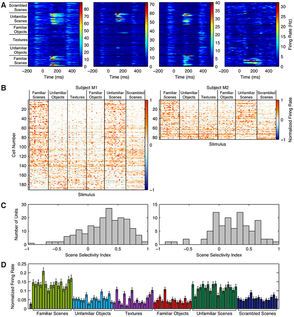
A, Response histograms for four example LPP single units. Cells 1 and 2 were recorded from M1; cells 3 and 4 were recorded from M2. B, Response profiles of visually responsive cells in LPP in M1 (left) and M2 (right), sorted by scene selectivity index. Each row represents one cell and each column one image. c, Histogram of scene selectivity indices for individual cells in M1 and M2. In both monkeys, the distribution was skewed toward positive values, indicating greater scene selectivity than would be expected by chance. D, Mean normalized response to each stimulus, averaged across all visually responsive cells. Scene stimuli evoked stronger activity than non-scene stimuli. Error bars are SEM. See also Figure S2.

Exploration of LPP connectivity by combined fMRI and microstimulation

Having confirmed that a large proportion of single units within LPP were scene-selective, we sought to investigate the connectivity of LPP with other regions by microstimulation. In M1 and M2, we advanced a low-impedance Pt-Ir electrode into LPP and verified that the multiunit activity we recorded was scene-selective (Figure S3A and S3B). We then placed the animal into the MRI, acquiring functional volumes while alternating between microstimulation on and microstimulation off conditions every 24 seconds while the monkey fixated on a centrally located dot. In both monkeys, microstimulation elicited strong activation throughout the OTS, as well as in an anatomically discontinuous region in the medial parahippocampal gyrus, which we term the medial place patch (MPP) for reasons discussed below. As with LPP, histological studies differ in their region labels for the area in which this activation resides, terming it TLO (Blatt and Rosene, 1998; Blatt et al., 2003), TFO (Saleem et al., 2007), or VTF (Boussaoud et al., 1991). Additional microstimulation-evoked activation was observed in extrastriate visual areas V4V and putative DP and in the inferior branch of the posterior middle temporal sulcus (PMTS) (Figure 3). In M1, we also observed activation in the posterior medial temporal sulcus. These areas are a subset of the areas identified by tracing studies in the vicinity of LPP, which have identified strong reciprocal connectivity with medial parahippocampal areas, as well as connectivity with extrastriate visual areas V3A, V3V, V4, FST, MST, LIP, and 7a; area TPO; retrosplenial cortex; and hippocampal subfield CA1 (Blatt and Rosene, 1998; Blatt et al., 2003; Distler et al., 1993). Our failure to observe activation in all of these regions could reflect lack of power of our microstimulation protocol to identify diffuse connections.

Figure 3:

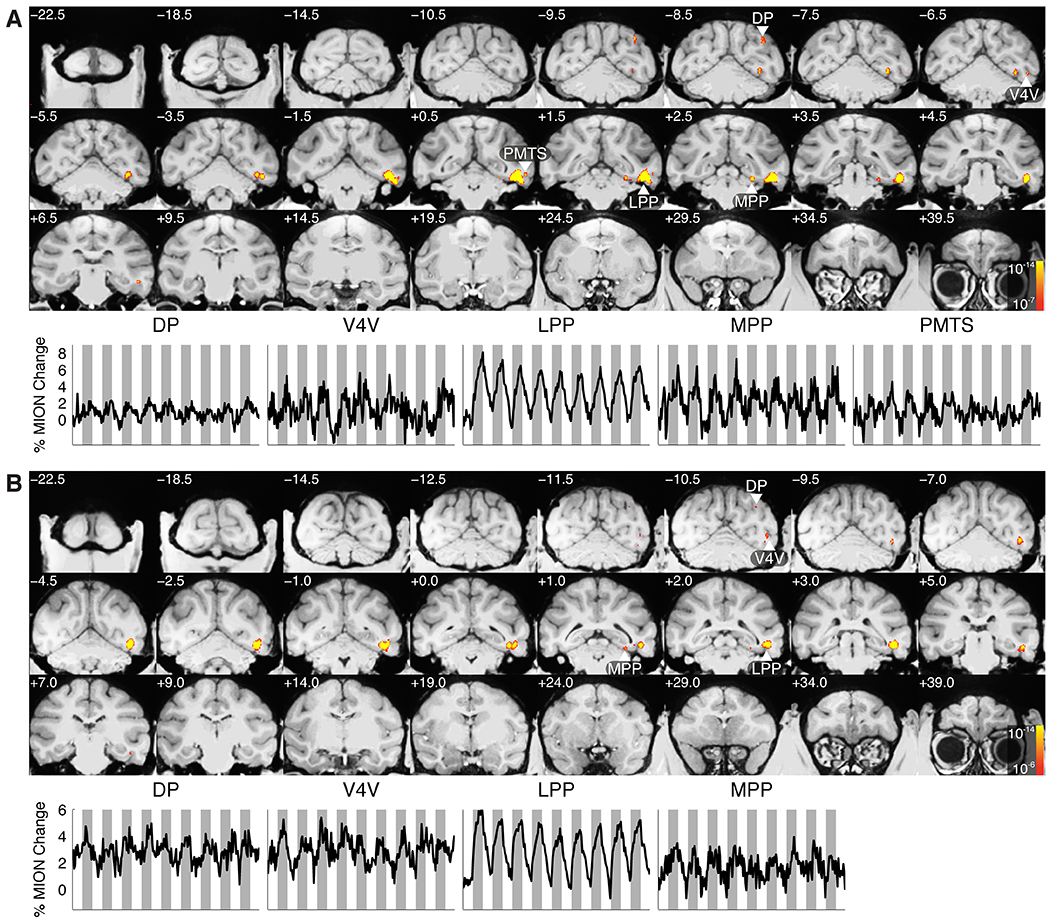
Areas showing significantly greater activation during microstimulation in the occipitotemporal place area as compared to baseline in subjects M1 (A) and M2 (B). Time courses for activated regions of interest are shown below the slice mosaic for each monkey. Shaded bars indicate time points during which microstimulation was active. Regions of interest were defined on one third of the data, while time courses were calculated from the remaining two thirds. See also Figure S3.

Scene selectivity of MPP

Of the areas activated observed by microstimulation, we were particularly interested in MPP. Because this area is putatively located within parahippocampal cortex, it is well suited to carry scene information to the hippocampus, and, like LPP, it is potentially homologous to the human PPA. Furthermore, the region was also weakly activated by the place localizer in one hemisphere of M3, suggesting that it might respond to passive viewing of scenes (Figure S1C). We targeted this medial parahippocampal region as activated by microstimulation in monkey M1 (Figures S4A and S4B) and recorded a large proportion of scene-selective single units (Figure 4A). 27% of visually responsive units (31/113) exhibited a scene selectivity index greater than ⅓ (median = 0.16; Figure 4B). While LPP and MPP exhibited similar latencies (LPP: 120 ± 42 ms; MPP: 123 ± 63 ms; p = 0.33, unequal variance t-test), the duration of the neural response was nearly twice as long in LPP as compared to MPP (LPP: 155 ± 76 ms; MPP: 90 ± 70 ms; p < 10⁻¹⁴, unequal variance t-test; Figure S4C). Additionally, none of 24 units recorded from grid holes immediately lateral to MPP were visually responsive, a significant difference from results in MPP (p = 0.002, Fisher’s exact test; Figures S4D–G). These results indicate that MPP and LPP are distinct functional regions.

Figure 4:

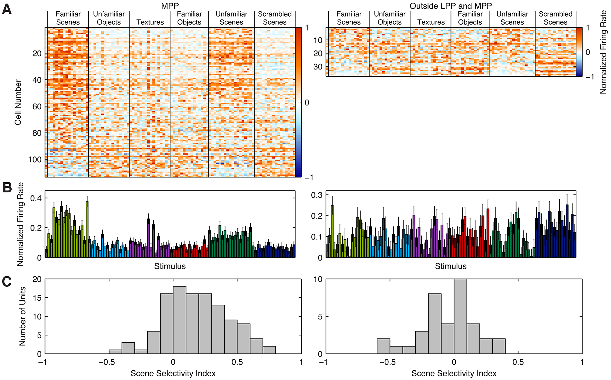
Single unit responses to scenes and non-scenes in MPP (left) and a control region posterior to LPP (right). A, Response profiles of recorded cells. Each row represents one cell and each column one image. B, Mean normalized response to each stimulus, averaged across all visually responsive cells. Scene stimuli evoked stronger activity than non-scene stimuli in MPP, but not the control region posterior to LPP. Error bars are SEM. C, Histogram of scene selectivity indices.

To ensure that the scene selectivity observed in single units in LPP and MPP was restricted to these regions, and not present throughout cortex, we also recorded from 41 single units in a region 3 mm posterior to LPP (Figures 4 and S4H). While 90% of cells (37/41) were visually responsive, only one exhibited a scene selectivity index greater than ⅓ (median = -0.01; Figure 4D), significantly fewer than in LPP (p < 10^-7, Fisher’s exact test) or MPP (p < 0.001). We also failed to observe scene selectivity in sites lateral to LPP and MPP (Figures S2C–F and S4D–G).

Since MPP clearly contains scene-selective units, we are uncertain why it was not strongly activated in our fMRI experiments localizing scene-selective regions in the brain (Figures 1 and S1). One possibility is that microstimulation and passive viewing both activate the same population of units in MPP, but that microstimulation evokes a stronger response in those units. Since the signal to noise ratio was slightly greater in LPP than MPP (Figure S3C), activation in the place localizer may not have been strong enough in MPP to achieve statistical significance at the single voxel level. We coregistered the MPP ROI activated microstimulation to the place localizer scanning sessions in each monkey and found that the mean beta values across the ROI indicated significant activation to scenes in M1 (p = 0.0057) and marginally significant activation in M2 (p = 0.059). A second factor may contribute to the discrepancy between our fMRI and single unit results: Unlike LPP, MPP contains a large population of cells that are not activated by passive viewing of scene stimuli, but which may be activated by microstimulation of LPP. Only 50% (113/228) of single units in MPP were visually responsive, versus 94% (275/294) in LPP (p < 10^-30, Fisher’s exact test). Finally, it is also possible that microstimulation activated neurons outside of MPP as well as in MPP itself, reducing partial volume effects. Our discovery of MPP as a scene-selective area underscores the importance of studying visual processing in terms of functionally connected networks, and confirms the power of fMRI combined with microstimulation as a tool to identify functionally connected networks (Ekstrom et al., 2008; Moeller et al., 2008; Tolias et al., 2005). Further studies with more advanced imaging technology will be necessary to confirm that visually evoked activity in MPP is consistently detectable by fMRI.

Population coding of individual scenes in LPP and MPP

We have shown that many individual LPP and MPP neurons respond more strongly to scenes than to non-scenes. This difference in mean response could indicate two possibilities (not mutually exclusive): first, these neurons could preferentially encode features that distinguish among scenes, and second, these neurons encode features that distinguish scenes from non-scenes. To examine these two possibilities, we trained naïve Bayes classifiers to discriminate between pairs of stimuli and to identify individual stimuli based on single presentation firing rates of groups of 25 visually responsive neurons in LPP, MPP, and the control region outside LPP (see Methods). We found that LPP neurons were equally accurate at discriminating scenes from other scenes and discriminating scenes from non-scenes (both 92%; p = 0.13, t-test), but significantly worse at discriminating non-scenes from other non-scenes (80%; both p < 10⁻⁵; Figure 5A and 5B). Responses of MPP neurons discriminated scenes from non-scenes slightly more accurately than they discriminated scenes from other scenes (scenes versus scenes: 79%; scenes versus non-scenes: 85%; p = 0.025), but were again substantially worse at distinguishing non-scenes from other non-scenes (61%; both p < 0.002). Moreover, cells in both regions were far more accurate at identifying individual scenes than at identifying individual non-scenes (LPP: 44% versus 16%; p < 10⁻¹³; MPP: 16% versus 4%; p < 10⁻⁹; Figure 5C).

Figure 5:

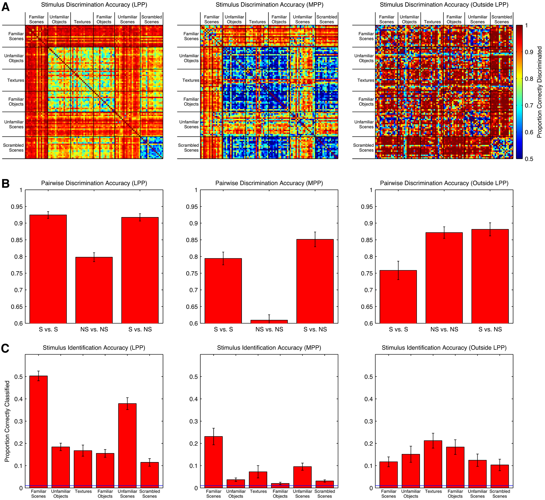
Performance of naïve Bayes classifiers in discriminating pairs of stimuli and identifying individual stimuli based on responses of 25 visually responsive single units in LPP (left), MPP (middle), and a control region posterior to LPP (right). A, Performance of classifier in distinguishing between pairs of stimuli. B, Average pairwise discrimination performance in each region for scenes versus scenes, non-scenes versus non-scenes, and scenes versus non-scenes. Chance performance is 50%. Error bars are SEM. C, Classifier accuracy in identifying individual stimuli from the full set of 98. Chance performance is 1%. Error bars are SEM.

To examine whether the observed differences in classification performance could be explained by differences in low-level similarity of the stimuli used, we performed two further controls. Using an HMAX C1 complex cell model, which approximates neural representation of images at the level of V1 (Riesenhuber and Poggio, 1999; Serre et al., 2007), we computed the Euclidean distance between responses of simulated complex cells to each of the images in our stimulus set. The distance between the responses to scene stimuli was not significantly different from than the distance between non-scene stimuli (scenes: 9.35 +/− 3.54, non-scenes: 8.87 +/− 2.31; p = 0.61, permutation test). Moreover, while classification performance based on neuronal responses of the control region outside LPP was also high, neurons within this region distinguished non-scenes from non-scenes and scenes from non-scenes more accurately than they distinguished scenes from scenes (scenes versus scenes: 78%, scenes versus non-scenes: 87%, scenes versus non-scenes: 89%; Figure 5A and 5B), and were slightly better at identifying non-scenes than scenes (12% versus 16%; Figure 5C).

Response modulation by long, straight contours in LPP and MPP

We used natural scene stimuli to localize LPP and to establish the scene selectivity of LPP and MPP via electrophysiological recording. While the use of such stimuli is common in neuroimaging literature, these stimuli differ appreciably in their low-level properties: A linear classifier trained on the output of the HMAX C1 complex cell model could easily distinguish scene and non-scene stimuli (Figure S5A). To further investigate the features represented by LPP neurons, we wanted to know which non-scene stimuli are most effective at driving scene-selective cells in LPP and MPP. We selected only scene-selective units (SSI > ⅓) in LPP and MPP, and sorted all of the stimuli within our localizer set by the average magnitude of the response among this population. Analysis of responses to non-scene stimuli revealed a key feature to which these cells respond: in both LPP and MPP, neurons tended to fire strongly to non-scene stimuli containing long, straight contours and weakly to stimuli containing short, curved contours (Figure 6A and B). For example, within the category of textures, the strongest responses were elicited by textures containing long straight contours, e.g., a series of vertically oriented tire treads, while weak responses were elicited by similarly regular textures lacking long contours, e.g., a mosaic of pebbles. The same pattern was observed in the local field potential: in response to most scenes, as well as to textures containing long, straight contours, the local field potential showed a distinctive response trough starting around 100 ms after stimulus onset that was smaller or not present in the response to other non-scenes (Figures 6C and D).

Figure 6:

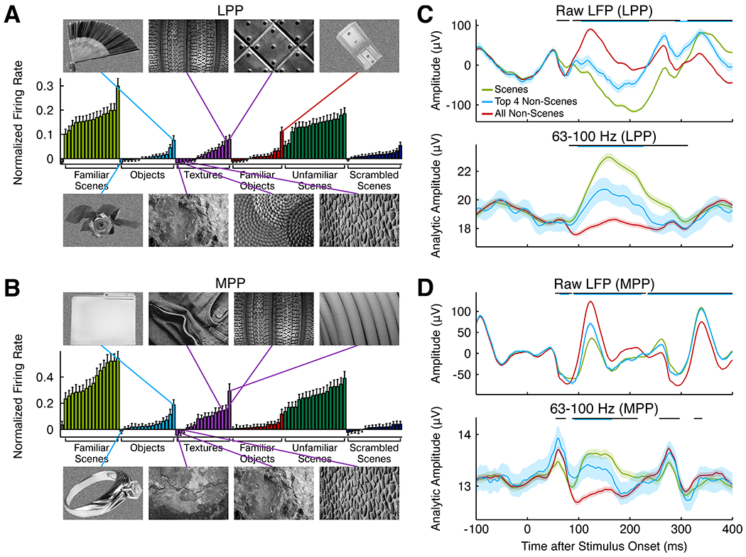
A and B, Mean normalized firing rate of visually responsive cells with scene selectivity index > ⅓ to each stimulus in the electrophysiology localizer in LPP (A) and MPP (B). Significant variance is visible in the magnitude of the mean response for non-scene stimuli. The four non-scene stimuli eliciting the strongest responses are shown above the graph; the four non-scene stimuli eliciting the weakest responses are shown below. C and D, Average LFP (top) and analytic amplitude in 63–100 Hz frequency band (bottom) to all scenes, top 4 non-scenes (shown to the left), and all non-scenes, averaged across 86 channels recorded from LPP (C) and 184 channels recorded from MPP (D). Error bars are 95% confidence intervals. Black strips at the top of each graph indicate significant differences between scenes and non-scenes; cyan strips indicate significant differences between the top and bottom four non-scenes (α = 0.001, t-test).

In order to provide a more objective assessment of modulation of LPP and MPP units by long, straight contours, using a merge sort algorithm, we asked 20 naïve human subjects to order the images by number of long, straight contours via a set of pairwise comparisons (see Methods). In both LPP and MPP, there was a significant correlation between the mean subject ranking and the rank of the mean response of scene-selective units (Figure S5B; LPP: r = 0.82, p < 10⁻²⁰, t-test; MPP: r = 0.82, p < 10⁻¹⁹; LPP versus MPP: p = 0.91, t-test for equality of two dependent correlations using Williams’s formula (Steiger, 1980)). This correlation remained highly significant when only non-scenes were included in the analysis (LPP: r = 0.64, p < 10⁻⁵; MPP: r = 0.53, p = 1.2×10⁻⁴; LPP versus MPP: p = 0.36). In MPP, but not LPP, the correlation was also significant when only scenes were included in the analysis (LPP: r = 0.18, p = 0.3; MPP: r = 0.50, p = 0.0025; LPP versus MPP: p = 0.014).

To determine whether scene selectivity in LPP and MPP is driven solely by long, straight contours, rather than by other characteristics of scenes, we computed a new scene selectivity index SSI_top by comparing responses to all scene stimuli against the seven non-scene stimuli that subjects had ranked as having the greatest numbers of long, straight contours (see Methods). In MPP, but not LPP, SSI_top was significantly less than SSI_all, the scene selectivity index computed using all non-scene stimuli (LPP: mean[SSI_all – SSI_top] = 0.028, p = 0.11, paired sample t-test; MPP: mean[SSI_all – SSI_top] = 0.078, p = 3.2×10⁻⁷; LPP versus MPP: p = 0.034, unequal variance t-test). In LPP, 42% (115/275) of visually responsive cells had a scene selectivity index of greater than ⅓ versus these seven scenes compared with 46% (127/275) against all scenes (p = 0.21, Liddell’s exact test). As a further control, we recorded from 13 cells in LPP while showing line drawings of scenes as well as disrupted versions of the same line drawings in which the lines had been randomly rotated or translated. Many but not all cells responded exclusively to the intact line drawings, suggesting that LPP represents spatial structure (Figure S5C–E). However, in MPP, only 14% (16/113) of visually responsive cells showed SSI_top > ⅓, compared with 27% (31/113) with SSI_all > ⅓, a significant reduction in selectivity (p = 0.004, Liddell’s exact test). These results indicate that units in MPP are more selective for long, straight contours and less selective to scenes per se than units in LPP. Nonetheless, MPP contains significantly more cells with SSI_top > ⅓ than the control region outside LPP (p = 0.027, Fisher’s exact test), suggesting that it may not be responding solely to contours.

It has previously been suggested that the PPA responds to high spatial frequencies (Rajimehr et al., 2011). We find no evidence for this. In both LPP and MPP, we found an inverse correlation between spatial frequency and average response magnitude that became insignificant once we included stimulus category in the regression (LPP: p = 0.10, ANOVA, MPP: p = 0.30, ANOVA; Figures S5F–G). Our results instead suggest a dominant feature driving both LPP and MPP responses is the presence of long, straight contours.

Encoding of scene boundaries and content in LPP and MPP

So far, we have demonstrated that cells in LPP and MPP respond selectively to scenes, but are driven to some degree by long, straight contours. The role of these contours in defining spatial boundaries and the comparable fMRI response of macaque LPP to rooms with and without objects (Figure 1 and S1) raise the possibility that cells in these regions might be coding topographical layout in a pure sense: i.e., they would respond the same to all scenes with the same spatial boundaries, regardless of wallpaper, furniture, etc. Alternatively, units might jointly encode scene content and scene boundaries. We thus sought to determine the sensitivity of unit responses in these areas to changes in boundary and content.

We constructed a stimulus set comprising images with 26 different spatial layouts. For each spatial layout, we constructed a line drawing that contained only the spatial boundaries of the scene (Figure 7A). To determine whether LPP cells encoded spatial layout information invariant to scene content, we recorded from 30 units while presenting both sets of stimuli. For each cell, we computed the Pearson correlation between the mean response to each of the original layouts and the line drawings representing those layouts. Correlation coefficients were significantly greater than a control distribution generated by permuting layout labels (p < 10⁻⁹, t-test; Figure 7B), indicating that LPP units carry some information about the spatial layout present in the stimulus independent of the content of the scene. Classification analysis confirmed this conclusion. We trained naïve Bayes classifiers using the responses to 4 presentations of each of the 28 scene photographs, and tested these classifiers on one presentation of each of the scene photographs that was not used to train the classifier along with one presentation of each of the line drawings. On average, the classifiers were 16% accurate at classifying line drawings based on the responses to the corresponding photographs, far better than chance (1/28 = 3.6%), but much worse than classifier performance on independent responses to the photographs (45%). Similarly, when trained on the line drawings, the classifiers were 17% accurate at classifying responses to the photographs, but 37% accurate classifying independent responses to the line drawings.

Figure 7:

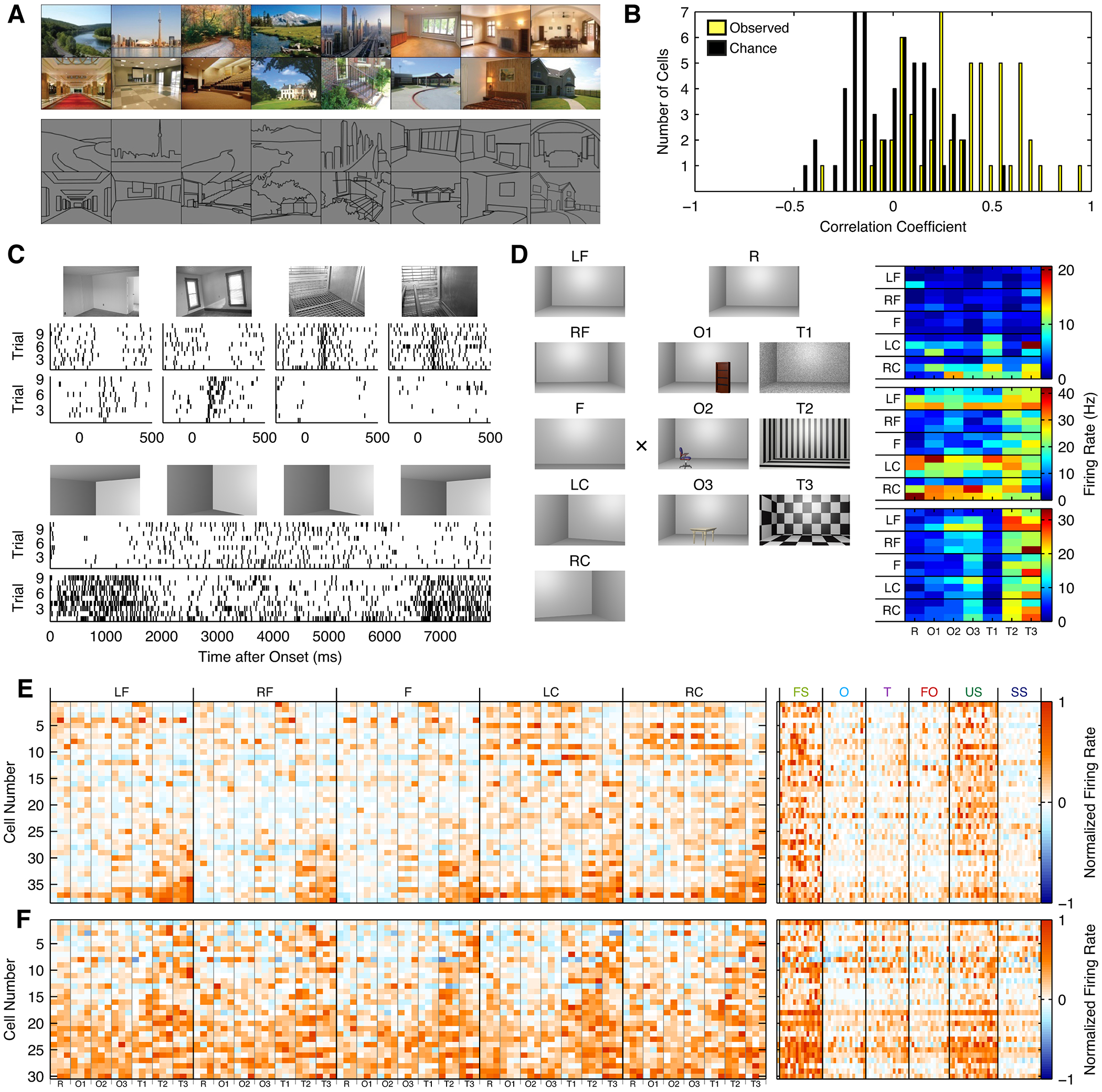
A, Examples of scene photographs (top) and corresponding line drawings (bottom) used. B, Histogram of the average correlation between photographs of scenes and line drawings of the same scenes. C, Two cells showing selectivity for images of top and bottom room corners (one cell/row). The top group of rasters show these cells responding to indoor scene images. The bottom group show the same two cells as in responding to top and bottom corners of a synthetic stimulus consisting of a 3D-rendered sequence panning from top to bottom to top of an empty room. D, Left: parameterized synthetic room stimuli. LF = front left; RF = front right; F = front; LC = left corner; RC = right corner; R = empty rooms; O = object; T = texture. Right: Three example cells from M1 demonstrating an interaction between response for texture and spatial viewpoint in parameterized synthetic room stimuli. Object and texture are shown on the x-axis, while viewpoint and depth are shown on the y-axis. E and F, Left: Response of scene-selective cells from M1 to the parameterized room stimuli from b in LPP (e) and MPP (f), sorted by the first principal component. Right: responses of the same cells to the place localizer stimuli. See also Figure S6.

While these results indicate that LPP neurons encode some information relevant to spatial layout regardless of scene content, they also imply that these cells are coding features unrelated to spatial layout. To further investigate the response properties of LPP and MPP neurons, we thus constructed a set of images of a single synthetic room that varied by viewpoint, depth, wall texture, and objects present in the scene (Figure S6A). We first determined that cells responded to synthetic room stimuli, and that the responses were similar to responses to the photographs used in our localizer. Figure 7C shows two cells in LPP with complementary response profiles that remained consistent across the localizer stimuli and a movie panning up and down in a 3D-rendered synthetic room, with one cell selective for images of a top room corner, and the other for images of a bottom room corner. At a population level, there was no significant difference in the responses to synthetic room stimuli and photographs of rooms (p = 0.49, ANOVA).

Next, we asked whether the cells in this region are modulated only by geometric parameters (depth and viewpoint), expected if they were used directly for navigation, or whether other visual features such as texture and objects also affect their responses, expected if they were used for scene recognition. We measured the response of 38 units in LPP (Figures 7D and 7E) and 30 units in MPP to static synthetic room stimuli (Figure 7F), presented stereoscopically in order to emphasize geometry, and performed a 4-way ANOVA to determine which factors modulated responses (Table 1). Crucially, no cells in either LPP or MPP were modulated by viewpoint or depth alone, expected if cells were coding pure spatial topography. Instead, for nearly all cells, a significant proportion of variance was explained by texture or objects present in the scene (α = 0.05, F-test; LPP: 35/38 units; MPP: 27/30 units). In both LPP and MPP, a significantly greater proportion of cells showed a main effect of texture than any other main effect or interaction (all p < 0.05, Liddell’s exact test). Nonetheless, in both LPP and MPP, the majority of cells were also modulated by viewpoint, depth, or an interaction involving viewpoint or depth (F-test; LPP: 32/38 units; MPP: 16/30 units; LPP vs. MPP: p = 0.008, Fisher’s exact test), and a minority of LPP neurons were much more strongly modulated by viewpoint or the interaction of viewpoint with depth than by other parameters (Figure S6B). In LPP, but not MPP, the majority of units were also modulated by object or an interaction involving it (LPP: 23/38 units; MPP: 6/30 units; LPP vs. MPP: p = 1×10⁻⁴). Classifiers trained on the responses of LPP neurons could classify all dimensions except for depth based on the responses to stimuli differing along each of the other dimensions with accuracy significantly above chance, indicating that information about viewpoint, texture, and object information is present at a population level (Figure S6C). In MPP, we also observed robust generalization of texture classification, as well as some generalization of classification of viewpoint and depth.

Table 1:

Proportions of visually responsive cells modulated by viewpoint, depth, object, and texture parameters in synthetic room stimuli, as determined by a 4-way ANOVA (α = 0.05). Because texture and object were not manipulated orthogonally, their interaction was not included in the model. Asterisks indicate significance of proportions versus chance determined by as determined by a binomial test (LPP and MPP columns) or significance of difference between regions as determined by Fisher’s exact test (Difference column).

	LPP (n = 38)	MPP (n = 30)	Difference
Viewpoint	53% ***	17% **	**
Depth	31% ***	10%	*
Object	58% ***	7%	***
Texture	92% ***	80% ***
Viewpoint × Depth	53% ***	13% *	***
Viewpoint × Object	24% ***	17% *
Viewpoint × Texture	66% ***	27% ***	**
Depth × Object	10% *	7%
Depth × Texture	47% ***	47% ***

^*= p < 0.05

^**= p < 0.01

^***= p < 0.001.

These findings demonstrate that neither LPP nor MPP are encoding pure spatial layout invariant to accompanying texture and objects. They also indicate a dissociation between LPP and MPP: while units in both areas were strongly modulated by texture, a larger proportion of LPP units were modulated by viewpoint, depth, and object identity. The large number of neurons modulated by texture may be partially attributable to greater visual dissimilarity. However, it is clear that LPP does not contain an invariant code for the location of spatial boundaries within a scene.

Representation of scene parts in LPP neurons

Scenes are generally composed of several components that intersect each other at spatial boundaries. The encoding of faces has been proposed to occur through population level coding of a face space, with individual cell selective for the presence of specific subsets of face parts (Freiwald et al., 2009). Could scenes be encoded in a similar way, by means of a combinatorial scene space? Specifically, are LPP neurons modulated by single parts of the scene, by a linear or non-linear combination of a small number of parts, or by all parts present? To investigate, we decomposed 11 scene images into their constituent parts and presented all possible part conjunctions while recording from neurons in LPP (Figure 8A). Figure 8B shows the responses of four example neurons to the scene eliciting the strongest overall response in the cells tested, which consisted an image of two cages broken down into five parts. Of the 84% of cells (21/25) modulated by the cage scene, over half (11/21) showed main effects of multiple scene parts (α = 0.05, ANOVA, Holm-corrected; p < 10⁻⁸, binomial test; Figure 8C). While main effects explained 79% of all stimulus-associated variance, 62% of responsive cells (13/21) also showed tuning to pairwise scene part interactions, explaining the majority of the remaining stimulus-associated variance (α = 0.05, ANOVA; p < 10⁻¹¹, binomial test). In total, 76% of responsive cells (16/21) were modulated by multiple scene parts, either as main effects or as pairwise interactions (combination of previous two tests performed at α = 0.025; p < 10⁻¹⁶, binomial test). Fewer units were tuned to third-order interactions (3/22 units; p = 0.09, binomial test), and no units were modulated by higher-order interactions. Thus, we restricted our analysis to main effects and pairwise interactions.

Figure 8:

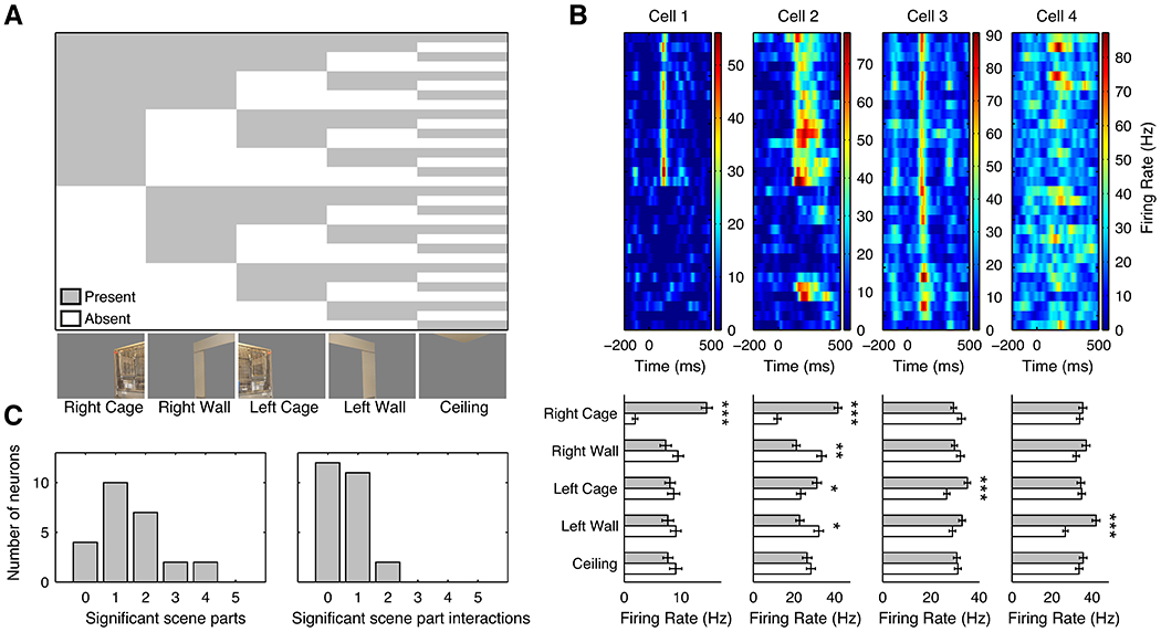
A, Stimulus conditions. An image of two sets of cages was separated into the right (contralateral) cage, right wall, left (ipsilateral) cage, left wall, and ceiling. All 31 combinations of five scene parts were shown. B, Top, average responses of four example cells to each combination of scene parts. Bottom, average responses in the presence (green bars) or absence (white bars) of a given scene parts. * = p < 0.05, ** = p < 0.01, *** = p < 0.001. Cell 1 responded only to the right cage. Cell 2 responded strongly to the right cage and weakly to the left cage when presented alone. Its response was inhibited by the presence of the left and right walls. Cell 3 responded to all stimulus parts except for the ceiling, but fired more strongly when the left cage was present. Cell 4 responded to the left wall. C, Distributions of the number of scene parts (left) and the number of pairwise interactions (right) that exerted a significant influence on cell firing for the cage scene for 25 cells (p < 0.05, Holm-corrected).

LPP units showed modulation by diverse aspects of the decomposed scenes, with selectivity patterns indicating integration of information across a large proportion of the visual field. 68% of cells (17/25) responded to the contralateral cage, more than for any other scene part (α = 0.05, ANOVA; p < 10⁻¹⁵, binomial test). However, significant numbers of units also responded to the contralateral wall (44%, 11/25), ipsilateral wall (36%, 9/25), and ipsilateral cage (32%, 8/25) (α = 0.05, ANOVA; all p < 10⁻⁴, binomial test). In total, 81% of cells modulated by the cage scene (17/21) were sensitive to ipsilaterally presented stimuli or interactions involving ipsilaterally presented stimuli (α = 0.05, ANOVA). Intriguingly, despite the large spatial separation between the two cages, the populations modulated by each showed significant overlap: 6 of the 8 cells responding to the ipsilateral cage responded to the contralateral cage as well, and 44% of cells (11/25) were modulated by the interaction between the cages. An insignificant number of cells (2/25) responded to the ceiling (α = 0.05, ANOVA; p = 0.35, binomial test), perhaps because it was not a prominent feature of the image, or because it is not a navigationally relevant feature.

Discussion

In this paper, we used a combination of fMRI, targeted electrical microstimulation, and single-unit electrophysiology to identify and functionally characterize two nodes within the network for processing visual scenes in the macaque brain. First, using fMRI, we identified the most robust activation to scene versus non-scene images within area LPP, a bilateral region in the fundus of the occipitotemporal sulcus anterior to area V4V. Next, microstimulation of LPP combined with simultaneous fMRI revealed that LPP is strongly connected to areas DP and V4V posteriorly, and to MPP, a discrete, more medial region within parahippocampal cortex located at the same anterior-posterior location as LPP. Finally, single-unit recordings targeted to LPP and MPP allowed us to characterize the selectivity of single cells within these two scene-selective regions to scene versus non-scene stimuli, as well as to a large number of different scene stimuli, revealing three major insights. First, the single-unit recordings showed that both regions contain a high concentration of scene-selective cells. Second, they showed that cells in both LPP and MPP exhibit a preference for stimuli containing long, straight contours, and responses of LPP neurons to photographs and line drawings of scenes are significantly correlated. Finally, experiments presenting two sets of combinatorially generated scene stimuli revealed a rich population code for scene content in LPP. Synthetic room stimuli multiplexing spatial factors (depth, viewpoint) with non-spatial factors (texture, objects) revealed that LPP cells are modulated not only by pure spatial factors but also by texture and objects, and decomposed scene stimuli revealed that individual LPP cells are selective for the presence of subsets of scene parts and part combinations.

In LPP and MPP, the average response across cells does not strongly depend upon the presence of objects, but instead depends upon the presence of spatial cues (Figures 1C, S1, 2, and 4). A similar result in the PPA led Epstein and Kanwisher (1998) to posit that the spatial-layout hypothesis: that the PPA “performs an analysis of the shape of the local environment that is critical to our ability to determine where we are.” In LPP, we found that responses to photographs of scenes correlate with responses line drawings of those same scenes, showing that neurons are tuned to specific layouts invariant to their content and providing additional support for the spatial-layout hypothesis. However, further experiments revealed that the spatial-layout hypothesis is an incomplete account of the information represented in LPP and MPP.

The responses of individual LPP and MPP neurons to systematically varied 3D renderings of a room containing objects show that these regions represent both spatial and non-spatial information, suggesting that their role extends beyond analysis of spatial layout. In both LPP and MPP, more cells were modulated by texture than by viewpoint, distance from walls, or objects present (Table 1), and most LPP neurons also represented information about objects present in the scene. While a significant number of neurons in both regions represented information about viewpoint and distance, either alone or in interaction with texture, no cells encoded only viewpoint or distance. Sensitivity to object ensemble and texture statistics has also been reported in the PPA (Cant and Goodale, 2011; Cant and Xu, 2012). Because texture is important for defining scene identity but irrelevant for specifying spatial layout, we suggest that LPP and MPP may selectively represent both spatial and non-spatial information about scenes in order to facilitate identification of specific locations.

Given that neurons in LPP and MPP respond to some non-scene images and do not represent high-level spatial layout invariant to texture, it is likely that these neurons, like other IT neurons, are tuned specific sets of complex shapes and visual features. LPP and MPP likely differ from other parts of IT not in the way they represent visual information, but their organization and the type of information they represent: these regions are macro-scale clusters of neurons showing selectivity for shapes and features present in scenes. Our scene and non-scene stimuli could be easily distinguished by a linear classifier trained on the output of the HMAX C1 complex cell model, suggesting that these scene and non-scene images (and perhaps most natural scene and non-scene images) are easily distinguishable from low-level features alone. The nature of the features to which LPP and MPP neurons respond, and their specificity to scenes, remains unresolved, although we suggest that specific configurations of long, straight lines may play an important role. We found that units in LPP and MPP respond more strongly to non-scene stimuli with such lines (Figure 6 and S5C–E). However, both LPP and MPP showed a greater proportion of scene-selective units than would be expected by chance when comparing scenes against only non-scenes with a large number of long, straight contours, and many LPP units showed selectivity for line drawings of scenes over disrupted arrangements of the same lines. While these results suggest that LPP neurons are tuned to linear features more complex than simple lines, we do not know the ultimate complexity of these features.

Although Rajimehr et al. (2011) have previously reported that the PPA responds selectively to images with high power at high spatial frequencies, we observed no correlation between high spatial frequency content and mean single neuron responses in LPP or MPP independent of stimulus category (Figures S5F–H). Because Rajimehr et al. (2011) based their conclusions on the PPA’s differential response to low-pass filtered images, in which sharp contours are blurred, and high-pass filtered images, in which sharp contours are accentuated, rather than by measuring the correlation between high spatial frequency content and PPA response to natural images, our results do not necessarily indicate a dissociation between LPP/MPP and the PPA. Further research will be necessary to determine whether the PPA responds selectively to non-scene images with long, straight contours.

Since positions and configurations of long, straight contours provide an egocentric, not allocentric, representation of spatial boundaries, if this information is naïvely represented in LPP and MPP, then neurons in these regions should display selectivity to viewpoint. Responses in LPP and MPP to the same synthetic room are modulated by the virtual viewpoint and depth from which the image was taken, supporting this view. Our results resemble fMRI results in the PPA, which show that a change in viewpoint produces a release from adaptation on a short timescale (Epstein et al., 2003, 2008; Park and Chun, 2009), although Epstein et al. (2008) have demonstrated that a viewpoint-invariant adaptation effect is present over longer timescales. However, since we did not vary room geometry, we cannot rule out the possibility that these regions nonetheless show partial viewpoint invariance. Indeed, the sensitivity of LPP and MPP to texture indicates that partial viewpoint invariance should be observed in natural scenes. Whether these neurons also show viewpoint invariance in scenes without differences in texture remains to be investigated.

How does LPP integrate information across the visual field? Our scene decomposition experiment revealed that the majority of LPP cells are modulated by multiple scene parts, often on both sides of the vertical meridian. However, just as few neurons in macaque middle face patches ML and MF are modulated by high-order interactions of face parts (Freiwald et al., 2009), few neurons in LPP were modulated by high-order interactions of scene parts. This may explain why LPP responds more strongly to fractured rooms that have been disassembled at spatial boundaries than to objects, a finding also observed in the PPA (Fig. 1; see Epstein and Kanwisher, 1998). We have not yet conducted these experiments in MPP; further work will be necessary to determine whether it displays similar receptive field and integrative properties.

While our experiments indicate that LPP and MPP share many properties, they also show several differences. First, while both LPP and MPP are scene-selective regions, both in their single unit responses (Figures 2B and 4A) and LFP (Figure 5), MPP contains a much greater proportion of non-visually responsive units, and a smaller proportion of visually responsive units are scene-selective (Figures 2C and 4B). Second, although our analysis showed that both LPP and MPP responded more strongly to non-scene stimuli with long, straight contours than to non-scene stimuli without such contours, the contribution of long, straight contours to scene selectivity in MPP was stronger than that in LPP. Finally, responses of both LPP and MPP neurons to systematically varied 3D-rendered scene stimuli are strongly modulated by texture, but MPP neurons show significantly weaker effects of viewpoint, depth, and object (Table 1). Together, these results indicate that LPP and MPP serve distinct roles in processing scenes, but their hierarchical relationship remains unclear. MPP’s reduced scene selectivity and greater selectivity for low-level features point toward a lower-level role in scene processing than LPP, but its more medial location and reduced object sensitivity suggest a higher-level role. Further experiments will be necessary to determine how LPP and MPP interact in scene processing.

Where are MPP and LPP? Although recent paracellations of macaque medial temporal lobe anatomy place MPP in posterior parahippocampal cortex, they conflict with regard to the anatomical label of LPP. The cytoarchitectonic paracellation of Saleem et al. (2007) puts LPP on the border between V4V and TEpv, and MPP in parahippocampal cortex, within a region they label TFO. Since most reviews of human PPA function rely upon this parcellation, we use its terminology for the remainder of the article. However, while Saleem et al. (2007) placed the lateral boundary of parahippocampal cortex several millimeters medial to the OTS, Blatt et al. (1998; 2003) have shown that retrograde tracer injections into a site in the medial bank of the OTS in approximately the same location as our LPP activations label a similar set of regions to more medial tracer injections cortex, including retrosplenial cortex and hippocampal subfield CA1. Their parcellation thus places both LPP and MPP within parahippocampal cortex, LPP within TFO and MPP within TLO.

While LPP and MPP are both within regions previously posited to hold the macaque homolog of the PPA, we emphasize that the current study is insufficient to establish homology. Anatomical studies and reviews have proposed that the macaque homolog of the PPA might span some combination of TFO (Epstein, 2008; Kravitz et al., 2011; Saleem et al., 2007; Sewards, 2011), TF/TH (Epstein, 2008; Kravitz et al., 2011; Saleem et al., 2007; Sewards, 2011), anterior V4V (Saleem et al., 2007), and TEpv (Sewards, 2011). Recently, Nasr et al. (2011) have argued that, based on its proximity to macaque face-selective areas, the macaque homolog of the PPA is in a scene-selective activation in the posterior middle temporal sulcus. While we found evidence for this activation (see Supplementary Results), we believe that the locations of LPP and MPP and their connectivity with medial temporal lobe regions known to be involved in navigation indicate that they are better candidates. Alternatively, all three regions may participate in scene processing. Further anatomical and functional characterization of these regions will be necessary to determine their relationship to human visual areas.

Although this paper investigates only the ventral aspect of the macaque scene processing network, fMRI and electrophysiology experiments including our own indicate that scene processing extends beyond the regions investigated. In our fMRI study, we observed consistent activation in putative V3A/DP, and LIP, and, in two of three animals, in the anterior parieto-occipital sulcus (APOS) adjoining V2, PGm, and v23b. All three of these activations were also present in the activation maps of Nasr et al. (2011). They suggested that the activation in putative V3A/DP corresponds to human TOS and the APOS activation corresponds to human retrosplenial cortex. While these homologies seem plausible, they are unproven. In particular, very little is known regarding the region in which the APOS activation resides, which is unlabeled in standard primate atlases (Paxinos et al., 2008; Saleem and Logothetis, 2012). The scene processing network likely terminates in the hippocampus, where, in macaques as in rodents, neurons represent space in an allocentric, stimulus-invariant manner (Ono et al., 1993; Rolls, 1999). While we anticipate that generating these allocentric representations requires input from LPP and MPP, further studies are necessary to verify this relationship.

Our experiments indicate that, while LPP and MPP are scene-selective, their responses multiplex both spatial and non-spatial information. We suggest that these areas, like the macaque middle face patches (Freiwald and Tsao, 2010), contain a population representation of viewpoint and identity. This representation may be useful in its own right for wayfinding in simple, well-learned environments, or it may give rise to a more invariant allocentric representation downstream when more complex topographical information is necessary to satisfy the demands of active navigation.

Experimental Procedures

All animal procedures used in this study complied with NIH, DARPA, and local guidelines. Three male rhesus macaques were implanted with MR-compatible head posts and trained to maintain fixation on a dot for a juice reward.

MRI.

Monkeys were scanned in a 3-tesla horizontal bore magnet (Siemens). Several T1-weighted anatomical volumes (MP RAGE; TR 2300 ms; IR 1100 ms; TE 3.37 ms; 256×256×240 imaging matrix; 0.5 mm isotropic voxels; 16–19 repetitions) acquired under dexmedetomidine anesthesia to obtain an anatomical volume of sufficient quality for surface reconstruction.

EPI volumes were acquired in an AC88 gradient insert (Siemens) while monkeys fixated on a central dot. Prior to the scan, monkeys were injected with ferumoxytol (Feraheme, AMAG Pharmaceuticals, 8 mg/kg), a formulation of dextran-coated iron oxide nanoparticles. Previous studies have demonstrated that iron oxide nanoparticle-based contrast agents increase contrast to noise and improve anatomical localization of the MR signal relative to BOLD (Vanduffel et al., 2001). During the scan, the monkey received juice every 3–5 seconds of continuous fixation.

For M1 and M2, imaging was performed with an 8-channel monkey coil (Massachusetts General Hospital) using parallel imaging (TR 2000 ms; TE 16 ms; 96×96 imaging matrix; 54 axial slices; 1 mm isotropic voxels; acceleration factor 2). For M3, due to technical issues, imaging was performed with a single-loop coil (TR 3000 ms; TE 20 ms; 96×96 imaging matrix; 54 axial slices; 1 mm isotropic voxels). During each scanning session, one or more field maps were acquired to correct for local magnetic field inhomogeneity and improve alignment of the functional scans with the anatomical scans. Figures 1 and S1 present data from a single session in M1 (13 runs) and M3 (19 runs), and an average of two sessions in M2 (19 runs). Figure 3 presents data from a single session (M1, 17 runs; M2, 16 runs).

Recording.

We drilled small superficial holes in the monkey’s implant under dexmedetomidine sedation and filled the holes with petroleum jelly to serve as MR-visible markers. Functional scans on which a region of interest had been defined were co-registered with anatomical scans showing these markers. Using custom software, we planned a chamber (Crist Instruments) to target the occipitotemporal place area and positioned and fastened it non-stereotaxically under dexmedetomidine anesthesia. After acquiring another anatomical volume to verify the location of the chamber and determine potential electrode trajectories, we made a craniotomy under ketamine/dexmedetomidine anesthesia.

Recordings were performed with a 0 degree plastic grid (Crist Instruments) using a guide tube cut to extend 3 mm below the surface of the dura according to the MR anatomical volume. A tungsten rod immersed in saline within the chamber served as a ground electrode. A hydraulic microdrive (Narishige) was used to advance a tungsten electrode (FHC) through the brain. After advancing the electrode quickly to 2–3 millimeters above the grey/white matter boundary of the occipitotemporal sulcus and allowing its depth to stabilize, we advanced slowly until an increase in multi-unit activity indicated entry into grey matter. We then attempted to isolate single units while advancing an additional 2–3 mm. All isolated single units were recorded regardless of firing rate or response characteristics. Spikes and local field potentials were digitized with a Plexon MAP system and saved for offline analysis.

Microstimulation.

We delivered 300 μA, 300 Hz charge-balanced bipolar current pulses for 200 ms at a rate of one pulse train per second while the monkey fixated on a centrally located dot on a grey screen. We simultaneously acquired functional volumes using the EPI sequence described above. 15 24-second blocks, 8 with and 9 without concomitant stimulation, were acquired per run. Stimulation pulses were delivered with a computer-triggered pulse generator (S88X, Grass Technologies) connected to a stimulus isolator (A365; World Precision Instruments).

Place localizer.

During imaging, stimuli were presented in 24-second blocks at an inter-stimulus interval of 500 ms. The localizer used to identify scene-selective regions during imaging consisted of five scene blocks and five non-scene blocks, as well as a block of fractured scenes and a block of line drawings of rooms (Figure S1). A block containing the same stimuli in grid-scrambled form preceded each stimulus block. Scene blocks consisted entirely of indoor scenes, either drawn from the monkey’s environment (two blocks), or from stock art collections and freely available images (three blocks). Objects were scaled to be as large as possible while maintaining their aspect ratio and superimposed on a background consisting of noise of uniformly distributed intensity. Three sets of stimuli were generated by superimposing several of familiar and unfamiliar objects over an intact scene, a scrambled scene, or a scene that had been filtered to preserve general intensity patterns while removing spatial boundary information. All blocks consisted of 16 images, except for the latter three sets, which consisted of 8. All images subtended approximately 23×15 degrees.

During recording, stimuli were presented for 100 ms, followed by a blank screen for 100 ms. Order was randomized. The stimulus set consisted of 16 images each of familiar scenes, scrambled scenes, familiar objects and textures; 15 images of familiar objects; 18 images of unfamiliar scenes; and a single image of uniform noise. Stimuli subtended approximately 55×39 degrees in order to provide an immersive visual display. However, a control experiment showed no significant difference in scene selectivity when the same stimuli were shown at 46×32 degrees or 35×24 degrees (p=0.70, Friedman’s test).

MRI data analysis.

Surface reconstruction based on anatomical volumes was performed using FreeSurfer (Massachusetts General Hospital). The brain was first isolated from the skull using FSL’s Brain Extraction Tool (University of Oxford). The resulting brain mask was refined manually. FreeSurfer’s automated brain segmentation was applied to the masked brain. The segmentation was further refined to ensure that it matched grey/white matter boundaries in the anatomical volume.

Analysis of functional volumes was performed using the FreeSurfer Functional Analysis Stream (Massachusetts General Hospital). Volumes were corrected for motion and undistorted based on acquired field map. Runs in which the norm of the residuals of a polynomial fit of displacement during the run exceeded 5 mm and the maximum displacement exceeded 0.55 mm were discarded. Our monkeys worked continuously throughout each scanning session before ceasing to fixate entirely, at which point we discarded the final run. The resulting data were analyzed using a standard general linear model. For the scene contrast, the average of all scene blocks was compared to the average of all non-scene blocks, ignoring the fractured scenes and outlined rooms. For the microstimulation contrast, the average of the blocks with concomitant stimulation was compared to the average of the blocks without stimulation. For the retinotopy contrast, the average of all blocks in which a horizontal wedge was shown was subtracted from the average of blocks in which a vertical wedge was shown.

Regions of interest were defined based on activations that were consistently observed in the same anatomical regions across subjects in one third of the data. All time courses and bar graphs displayed were generated from the remaining two thirds.

Electrophysiological data analysis.

To compute the response to each image in the stimulus set, we averaged the number of spikes over the time window from 100 ms to 250 ms after stimulus onset (LPP) or 75 to 150 ms after stimulus onset (MPP). Trials in which the monkey did not fixate in a central window of ±2 degrees (±1 degree for eccentricity mapping) were discarded, as were results from cells for which the median number of valid presentations per stimulus fell below six (M1: mean number of presentations 10.0 +/− 0.9, M2: 11.7 +/− 1.0). We calculated the baseline activity on a per-cell basis as the minimum of any 25 ms bin spanning the period from 150 before stimulus onset to the start of the response window. For the population plots (Figure 2B, Figure 4B), we subtracted the baseline activity and divided by the maximum response. Visual responsiveness was assessed as differential firing to different stimuli that was significant in a Kruskal-Wallis ANOVA (α = 0.05). Non-visually responsive units were excluded from further analysis.

Classification analysis was performed using naïve Bayes classifiers assuming a multivariate normal density and equal variance for responses to all stimuli. Classifiers were first trained using responses to four presentations of each stimulus. Pairwise discrimination accuracy was tested by finding the stimulus out of the pair with the greatest posterior probability. Identification was performed by finding the stimulus out of the entire stimulus set with the greatest posterior probability. This procedure was repeated for 1000 subsets of 25 visually responsive cells for which we recorded at least five valid trials for each stimulus on each the five possible partitions of four training trials and one test trial. The percentages shown in Figure 5 were calculated as the number of successful classifications out of a possible five, averaged over the 1000 subsets.

Local field potentials were band-pass filtered between 0.7 Hz and 170 Hz prior to acquisition at 1000 Hz and averaged across sessions and recording sites. Because recording problems occasionally resulted in persistent large artifacts in the local field potential, only cells for which the standard deviation of the LFP across stimulus presentations averaged over stimuli and time points fell below 300 μV were included in the LFP average. Analytic amplitude was computed as the magnitude of the Hilbert transform of the band-pass filtered LFP (Freeman, 2004). LFPs were band-pass filtered using a 100 sample FIR filter with pass and stop-band widths of 5 Hz.

Subjective ranking of image contours.

In order to determine the degree to which the presence of long, straight contours modulates the population response in LPP and MPP, we created a paradigm to construct an ordering of the 72 non-scramble stimuli in the place localizer set we used for electrophysiology via a merge sort with a manual comparison function. Subjects saw two images simultaneously and had to click the image that contained a greater number of long, straight contours for approximately 400 pairs. 20 participants were recruited through Amazon Mechanical Turk (MTurk), which has previously been shown to match or exceed reliability of traditional psychological testing methods (Buhrmester et al., 2011). We required that subjects had performed at least 1000 previous Amazon Mechanical Turk HITs (human intelligence tasks), and that at least 95% of previous HITs were accepted by their requesters. Data from one subject whose reaction times were implausibly low was discarded.

To determine the number of stimuli to use to compute SSI_top, we determined the subjective contour ranking value that maximizes the separation between scenes and non-scenes (i.e., if all stimuli greater than a threshold are classified as scenes, and all stimuli less than a threshold are classified as non-scenes, we selected the threshold value that minimizes the classification error). The seven non-scene stimuli used had subjective contour rankings greater than this threshold value. The mean contour rank of the seven top non-scene long contour stimuli was 53.7 +/− 6.4, versus 56.6 +/− 8.0 for the scenes.

Synthetic room experiment.

We constructed synthetic room stimuli using commercially available 3D modeling software (Blender; Blender Foundation) from different 5 viewpoints at 3 depths, and with one of 3 textures superimposed over the walls or one of 3 objects presented in the foreground. Textures tested included both simple patterns (checkerboards, vertical lines, and uniform random noise) and objects superimposed as wallpaper. The full set of stimuli presented is shown in Figure S6. The images were presented stereoscopically using two projectors equipped with polarizing filters configured to project to the same screen. The monkey wore polarized glasses during presentation. Stimuli subtended approximately 55×33 degrees.

The obtained responses were analyzed by ANOVA using type III sum of squares. The design included main effects of viewpoint, depth, object, and texture, along with pairwise interactions viewpoint × depth, viewpoint × object, viewpoint × texture, depth × object, and depth × texture. Because we did not orthogonally manipulate object and texture, we could not measure the interaction between these two factors. Variability was calculated over individual presentations of each stimulus.

Scene decomposition experiment.

We chose 11 scenes spanning a wide variety of parameters, including outdoor versus indoor, familiar versus unfamiliar, and real vs. virtual. We decomposed each scene into 3 to 5 parts according to the surface boundaries and created scenes representing all 2^N-1 possible combinations of the scene parts, with the missing parts in each scene replaced by a neutral gray background. A total of 253 scene images were presented. Stimuli subtended approximately 55×43 degrees.

Highlights.

• fMRI localized a scene-selective area in the occipitotemporal sulcus (LPP)

• Microstimulation of LPP activated a second, more medial scene-selective area (MPP)

• Neurons respond more strongly to non-scenes with long, straight contours

• Neurons are modulated by both spatial and non-spatial factors

References

- Aguirre GK, and D’Esposito M (1999). Topographical disorientation: a synthesis and taxonomy. Brain 122, 1613. [DOI] [PubMed] [Google Scholar]
- Blatt GJ, and Rosene DL (1998). Organization of direct hippocampal efferent projections to the cerebral cortex of the rhesus monkey: Projections from CA1, prosubiculum, and subiculum to the temporal lobe. J. Comp. Neurol 392, 92–114. [DOI] [PubMed] [Google Scholar]
- Blatt GJ, Pandya DN, and Rosene DL (2003). Parcellation of cortical afferents to three distinct sectors in the parahippocampal gyrus of the rhesus monkey: An anatomical and neurophysiological study. J. Comp. Neurol 466, 161–179. [DOI] [PubMed] [Google Scholar]
- Boussaoud D, Desimone R, and Ungerleider LG (1991). Visual topography of area TEO in the macaque. J. Comp. Neurol 306, 554–575. [DOI] [PubMed] [Google Scholar]
- Buhrmester M, Kwang T, and Gosling SD (2011). Amazon’s Mechanical Turk: A new source of inexpensive, yet high-quality, data? Perspect. Psychol. Sci 6, 3–5. [DOI] [PubMed] [Google Scholar]
- Cant JS, and Goodale MA (2011). Scratching beneath the surface: new insights into the functional properties of the lateral occipital area and parahippocampal place area. J. Neurosci 31, 8248–8258. [DOI] [PMC free article] [PubMed] [Google Scholar]
- Cant JS, and Xu Y (2012). Object ensemble processing in human anterior-medial ventral visual cortex. J. Neurosci 32, 7685–7700. [DOI] [PMC free article] [PubMed] [Google Scholar]
- Dilks DD, Julian JB, Kubilius J, Spelke ES, and Kanwisher N (2011). Mirror-image sensitivity and invariance in object and scene processing pathways. J. Neurosci 31, 11305–11312. [DOI] [PMC free article] [PubMed] [Google Scholar]
- Distler C, Boussaoud D, Desimone R, and Ungerleider LG (1993). Cortical connections of inferior temporal area TEO in macaque monkeys. J. Comp. Neurol 334, 125–150. [DOI] [PubMed] [Google Scholar]
- Ekstrom LB, Roelfsema PR, Arsenault JT, Bonmassar G, and Vanduffel W (2008). Bottom-up dependent gating of frontal signals in early visual cortex. Science 321, 414–417. [DOI] [PMC free article] [PubMed] [Google Scholar]
- Epstein RA (2008). Parahippocampal and retrosplenial contributions to human spatial navigation. Trends Cogn. Sci 12, 388–396. [DOI] [PMC free article] [PubMed] [Google Scholar]
- Epstein R, and Kanwisher N (1998). A cortical representation of the local visual environment. Nature 392, 598–601. [DOI] [PubMed] [Google Scholar]
- Epstein R, Harris A, Stanley D, and Kanwisher N (1999). The parahippocampal place area: recognition, navigation, or encoding? Neuron 23, 115–125. [DOI] [PubMed] [Google Scholar]
- Epstein R, DeYoe EA, Press DZ, Rosen AC, and Kanwisher N (2001). Neuropsychological evidence for a topographical learning mechanism in parahippocampal cortex. Cogn Neuropsychol 18, 481–508. [DOI] [PubMed] [Google Scholar]
- Epstein R, Graham KS, and Downing PE (2003). Viewpoint-specific scene representations in human parahippocampal cortex. Neuron 37, 865–876. [DOI] [PubMed] [Google Scholar]
- Epstein RA, Parker WE, and Feiler AM (2008). Two kinds of fMRI repetition suppression? Evidence for dissociable neural mechanisms. J Neurophysiol 99, 2877–2886. [DOI] [PubMed] [Google Scholar]
- Freeman WJ (2004). Origin, structure, and role of background EEG activity. Part 1. Analytic amplitude. Clin. Neurophysiol 115, 2077–2088. [DOI] [PubMed] [Google Scholar]
- Freeman J, Brouwer GJ, Heeger DJ, and Merriam EP (2011). Orientation decoding depends on maps, not columns. J. Neurosci 31, 4792–4804. [DOI] [PMC free article] [PubMed] [Google Scholar]
- Freiwald WA, and Tsao DY (2010). Functional compartmentalization and viewpoint generalization within the macaque face-processing system. Science 330, 845–851. [DOI] [PMC free article] [PubMed] [Google Scholar]
- Freiwald WA, Tsao DY, and Livingstone MS (2009). A face feature space in the macaque temporal lobe. Nat. Neurosci 12, 1187–1196. [DOI] [PMC free article] [PubMed] [Google Scholar]
- Hafting T, Fyhn M, Molden S, Moser M-B, and Moser EI (2005). Microstructure of a spatial map in the entorhinal cortex. Nature 436, 801–806. [DOI] [PubMed] [Google Scholar]
- Harel A, Kravitz DJ, and Baker CI (2012). Deconstructing Visual Scenes in Cortex: Gradients of Object and Spatial Layout Information. Cereb. Cortex [DOI] [PMC free article] [PubMed] [Google Scholar]
- Kravitz DJ, Saleem KS, Baker CI, and Mishkin M (2011). A new neural framework for visuospatial processing. Nat. Rev. Neurosci 12, 217–230. [DOI] [PMC free article] [PubMed] [Google Scholar]
- MacEvoy SP, and Epstein RA (2007). Position Selectivity in Scene- and Object-Responsive Occipitotemporal Regions. J. Neurophysiol 98, 2089–2098. [DOI] [PubMed] [Google Scholar]
- Mendez MF, and Cherrier MM (2003). Agnosia for scenes in topographagnosia. Neuropsychologia 41, 1387–1395. [DOI] [PubMed] [Google Scholar]
- Moeller S, Freiwald WA, and Tsao DY (2008). Patches with links: A unified system for processing faces in the macaque temporal lobe. Science 320, 1355–1359. [DOI] [PMC free article] [PubMed] [Google Scholar]
- Moser EI, Kropff E, and Moser M-B (2008). Place cells, grid cells, and the brain’s spatial representation system. Annu. Rev. Neurosci 31, 69–89. [DOI] [PubMed] [Google Scholar]
- Nasr S, Liu N, Devaney KJ, Yue X, Rajimehr R, Ungerleider LG, and Tootell RBH (2011). Scene-selective cortical regions in human and nonhuman primates. J. Neurosci 31, 13771–13785. [DOI] [PMC free article] [PubMed] [Google Scholar]
- O’Keefe J, and Conway DH (1978). Hippocampal place units in the freely moving rat: why they fire where they fire. Exp. Brain Res. Exp. Hirnforsch. Expérimentation Cérébrale 31, 573–590. [DOI] [PubMed] [Google Scholar]
- Ono T, Nakamura K, Nishijo H, and Eifuku S (1993). Monkey hippocampal neurons related to spatial and nonspatial functions. J. Neurophysiol 70, 1516–1529. [DOI] [PubMed] [Google Scholar]
- Park S, and Chun MM (2009). Different roles of the parahippocampal place area (PPA) and retrosplenial cortex (RSC) in panoramic scene perception. NeuroImage 47, 1747–1756. [DOI] [PMC free article] [PubMed] [Google Scholar]
- Paxinos G, Huang X-F, Petrides M, and Toga AW (2008). The rhesus monkey brain in stereotaxic coordinates (London: Academic Press; ). [Google Scholar]
- Rajimehr R, Devaney KJ, Bilenko NY, Young JC, and Tootell RBH (2011). The “parahippocampal place area” responds preferentially to high spatial frequencies in humans and monkeys. Plos Biol. 9, e1000608. [DOI] [PMC free article] [PubMed] [Google Scholar]
- Riesenhuber M, and Poggio T (1999). Hierarchical models of object recognition in cortex. Nat. Neurosci 2, 1019–1025. [DOI] [PubMed] [Google Scholar]
- Rolls ET (1999). Spatial view cells and the representation of place in the primate hippocampus. Hippocampus 9, 467–480. [DOI] [PubMed] [Google Scholar]
- Rosenbaum RS, Ziegler M, Winocur G, Grady CL, and Moscovitch M (2004). “I have often walked down this street before”: fMRI Studies on the hippocampus and other structures during mental navigation of an old environment. Hippocampus 14, 826–835. [DOI] [PubMed] [Google Scholar]
- Saleem KS, and Logothetis NK (2012). A Combined MRI and Histology Atlas of the Rhesus Monkey Brain in Stereotaxic Coordinates, Second Edition (London: Academic Press; ). [Google Scholar]
- Saleem KS, Price JL, and Hashikawa T (2007). Cytoarchitectonic and chemoarchitectonic subdivisions of the perirhinal and parahippocampal cortices in macaque monkeys. J. Comp. Neurol 500, 973–1006. [DOI] [PubMed] [Google Scholar]
- Sawamura H, Orban GA, and Vogels R (2006). Selectivity of neuronal adaptation does not match response selectivity: a single-cell study of the fMRI adaptation paradigm. Neuron 49, 307–318. [DOI] [PubMed] [Google Scholar]
- Serre T, Oliva A, and Poggio T (2007). A feedforward architecture accounts for rapid categorization. Proc. Natl. Acad. Sci 104, 6424–6429. [DOI] [PMC free article] [PubMed] [Google Scholar]
- Sewards TV (2011). Neural structures and mechanisms involved in scene recognition: A review and interpretation. Neuropsychologia 49, 277–298. [DOI] [PubMed] [Google Scholar]
- Steiger JH (1980). Tests for comparing elements of a correlation matrix. Psychol. Bull 87, 245–251. [Google Scholar]
- Takahashi N, Kawamura M, Shiota J, Kasahata N, and Hirayama K (1997). Pure topographic disorientation due to right retrosplenial lesion. Neurology 49, 464–469. [DOI] [PubMed] [Google Scholar]
- Taube JS, Muller RU, and Ranck JB (1990). Head-direction cells recorded from the postsubiculum in freely moving rats. II. Effects of environmental manipulations. J. Neurosci 10, 436–447. [DOI] [PMC free article] [PubMed] [Google Scholar]
- Tolias AS, Sultan F, Augath M, Oeltermann A, Tehovnik EJ, Schiller PH, and Logothetis NK (2005). Mapping cortical activity elicited with electrical microstimulation using FMRI in the macaque. Neuron 48, 901–911. [DOI] [PubMed] [Google Scholar]
- Tsao DY, Freiwald WA, Knutsen TA, Mandeville JB, and Tootell RBH (2003). Faces and objects in macaque cerebral cortex. Nat. Neurosci 6, 989–995. [DOI] [PMC free article] [PubMed] [Google Scholar]
- Tsao DY, Freiwald WA, Tootell RBH, and Livingstone MS (2006). A cortical region consisting entirely of face-selective cells. Science 311, 670–674. [DOI] [PMC free article] [PubMed] [Google Scholar]
- Ungerleider LG, Galkin TW, Desimone R, and Gattass R (2008). Cortical connections of area V4 in the macaque. Cereb. Cortex 18, 477–499. [DOI] [PubMed] [Google Scholar]
- Vanduffel W, Fize D, Mandeville JB, Nelissen K, Van Hecke P, Rosen BR, Tootell RB., and Orban GA (2001). Visual motion processing investigated using contrast agent-enhanced fMRI in awake behaving monkeys. Neuron 32, 565–577. [DOI] [PubMed] [Google Scholar]
- Yoder RM, Clark BJ, and Taube JS (2011). Origins of landmark encoding in the brain. Trends Neurosci. 34, 561–571. [DOI] [PMC free article] [PubMed] [Google Scholar]
Associated Data
This section collects any data citations, data availability statements, or supplementary materials included in this article.