Multi-Domain Image Completion for Random Missing Input Data

Abstract

Multi-domain data are widely leveraged in vision applications taking advantage of complementary information from different modalities, e.g., brain tumor segmentation from multi-parametric magnetic resonance imaging (MRI). However, due to possible data corruption and different imaging protocols, the availability of images for each domain could vary amongst multiple data sources in practice, which makes it challenging to build a universal model with a varied set of input data. To tackle this problem, we propose a general approach to complete the random missing domain(s) data in real applications. Specifically, we develop a novel multi-domain image completion method that utilizes a generative adversarial network (GAN) with a representational disentanglement scheme to extract shared content encoding and separate style encoding across multiple domains. We further illustrate that the learned representation in multi-domain image completion could be leveraged for high-level tasks, e.g., segmentation, by introducing a unified framework consisting of image completion and segmentation with a shared content encoder. The experiments demonstrate consistent performance improvement on three datasets for brain tumor segmentation, prostate segmentation, and facial expression image completion respectively.

I. Introduction

MULTI-DOMAIN images are often required as inputs in various vision tasks because of the nature that different domains could provide complementary knowledge. For example, four medical imaging modalities, MRI with T1, T1-weighted, T2-weighted, FLAIR (FLuid-Attenuated Inversion Recovery), are acquired as a standard protocol to accurately segment the tumor regions for each patient in the brain tumor segmentation task [1]. Different modalities provide distinct features to locate tumor boundaries from differential diagnosis perspectives. Additionally, when it comes to the natural image tasks, there are similar scenarios such as person re-identification across different cameras or times [2], [3]. Here, the medical images in different modalities or natural images with the person under varied appearances can be considered as different image domains, depicting the same underlying subject or scene from various aspects.

However, some image domains might be missing in practice. Especially when it comes to a large-scale multi-institute study, it is generally difficult or even infeasible to guarantee the availability of data in all domains for every data entry. For example, some patients might lack certain imaging scans due to different imaging protocols, data loss or image corruption. For these rare and valuable collected data, it is costly to just throw away the incomplete samples during training, and also infeasible to test with missing-domain inputs. Thus, in order to take the most advantage of such missing data, it becomes crucial to design an effective data completion algorithm to cope with this challenge. An intuitive approach is to impute the missing domain of one sample with the nearest neighbor from other samples whose corresponding domain image exists. But this might lack of semantic consistency among different domains of the input sample as shown in Fig. 2 since it only focuses on the pixel-level similarity compared with existing images. Another possible solution is to generate images and complete missing domains via image translation from existing domains using generative models, such as GAN models, as illustrated in Fig. 1.

Fig. 2.

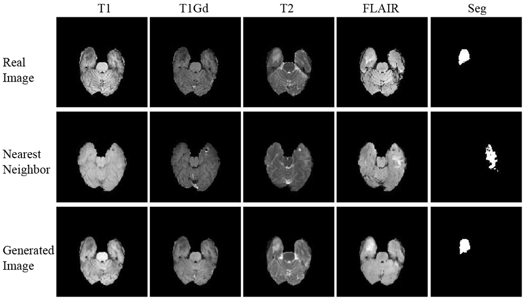
BraTS images in four modalities with nearest neighbors and generated images from the proposed method (ReMIC). From the segmentation prediction of brain tumor, the generated images preserve better semantic consistency with ground truth in addition to the pixel-level similarity in images.

Fig. 1.

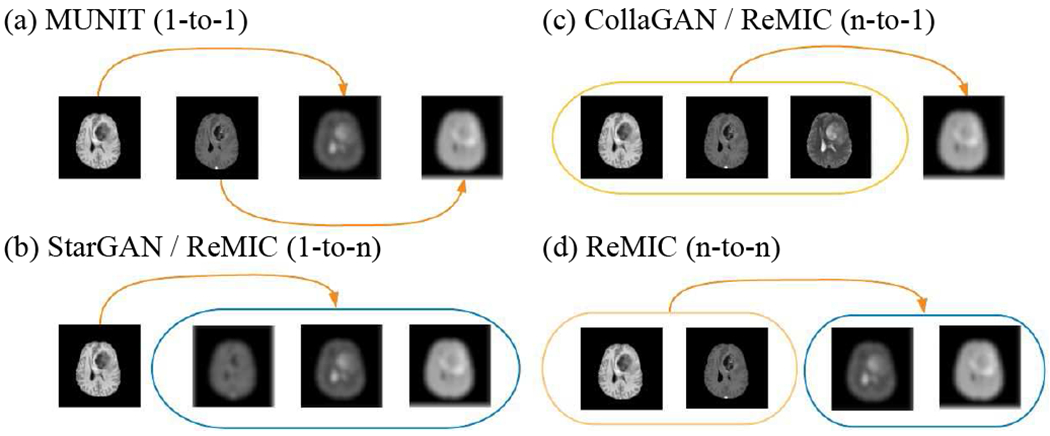
Image translation using (a) MUNIT (1-to-1), (b) StarGAN / Ours (ReMIC) (1-to-n), (c) CollaGAN / ReMIC (n-to-1), and (d) ReMIC (n-to-n). In multi-domain image completion, Ours (ReMIC) completes the missing-domain images given randomly distributed numbers (k-to-n, 1 ≤ k ≤ n) of visible domains in the input. Note the missing-domain images are denoted as blurred images.

In this work, we propose a general n-to-n image completion framework based on a Representational disentanglement scheme for Multi-domain Image Completion (ReMIC). Specifically, our contribution is fourfold: (1) We propose a novel GAN framework for a general and flexible n-to-n image generation with representational disentanglement, i.e., learning semantically shared representations cross domains (content code) and domain-specific features (style code) for each input domain; (2) We demonstrate the learned content code could be utilized for the high-level task, i.e., developing a unified framework for jointly learning the image completion and segmentation based on shared content encoder; (3) We demonstrate the proposed n-to-n image generation model can effectively completes the missing domains given randomly distributed numbers (k-to-n, 1 ≤ k ≤ n) of visible domains in the input; (4) Experiments on three datasets illustrate that the proposed method consistently achieves better performance than previous approaches in both multi-domain image completion and missing-domain segmentation.

II. Related Work

A. Image-to-Image Translation

The recent success of GANs [4–16] in image-to-image translation provides a promising solution to deal with the challenge of missing image domains. CycleGAN [7] shows impressive performance in image-to-image translation via cycle-consistency between real and generated images. However, it mainly focuses on 1-to-1 mapping between two domains and assumes corresponding images in two domains strictly share the same representation in latent space. This is limited in multi-domain applications since $\frac{n\left(n-1\right)}{2}$ CycleGAN models are required if there are n domains. Following this, StarGAN [11] proposes to use a mask vector in inputs to specify the desired target domain in multi-domain image generation. Meantime, RadialGAN [12] also deals with the multi-domain generation problem by assuming all the domains share the same latent space. Although these works make it possible to generate images in different target domains through 1-to-n mapping with multiple inference passes, the representation learning and image generation are always conditioned on the single input image as the only source domain. In order to take advantage of multiple available domains, CollaGAN [13] proposes a collaborative model to incorporate multiple domains for generating one missing domain. Similar to StarGAN, CollaGAN relies on the cycle-consistency to preserve the contents in the generated images, which is an indirect and implicit constraint for target domain images. Additionally, since the target domain is specified by an one-hot mask vector in input, CollaGAN is essentially doing n-to-1 translation with a single output in an one-time inference. As illustrated in Fig. 1, our proposed model is a more general n-to-n image generation framework that can overcome aforementioned limitations.

B. Learning Disentangled Representations

Recently, learning disentangled representations is proposed to capture the full distribution of possible outputs by introducing a random style code [17–22], or to transfer information across domains for adaptation [23], [24], InfoGAN [17] and β-VAE [18] learn the disentangled representation in an unsupervised manner. In image translation, DRIT [20] disentangles content and attribute features by exchanging the features encoded from two domains respectively. The image consistency during translation is constrained by the code and image reconstruction. With a similar code exchange scheme, MUNIT [19] assumes a prior distribution on style code, which allows directly sampling style codes from the prior distribution to generate target domain images. However, both DRIT and MUNIT only deal with image translation between two domains, which requires to independently train $\frac{n\left(n-1\right)}{2}$ separate translation models among n domains. While the recent work [24] also tackles multi-domain image translation, it focuses more on learning cross-domain latent code for domain adaptation with less discussion about the domain-specific style code. Moreover, our proposed method handles a more challenging problem with random missing domains motivated by practical medical applications. Aiming at higher completion accuracy for the segmentation task with missing domains, we further add reconstruction and segmentation constraints in our framework.

C. Medical Image Synthesis

Synthesizing medical images has attracted increasing interests in recent researches [14–16], [25–31]. The synthesized images are generated across multi-contrast MRI modalities or between MRI and computed tomography (CT) [32–34]. Other works [35–37] also discuss how to extract representations from multi-modalities especially for segmentation with missing imaging modalities. However, these studies mostly focus on how to fuse the features from multiple modalities but not from the perspective of representation disentanglement. Our model disentangles the shared content and separate style representations for a more general n-to-n multi-domain image completion task, and we further validate that the generation benefits the segmentation task.

III. Method

Images from different domains for the same sample present their exclusive features of the subject. Nonetheless, they also inherit some global content structures. For instance, in the parametric MRI for brain tumors, T2 and FLAIR MRI highlight the differences in tissues’ water relaxational properties, which will distinguish the tumor tissue from normal ones. Contrasted T1 MRI can examine the pathological intratumoral take-up of contrast agents so that the boundary between tumor core and the rest will be highlighted. However, the underlying anatomical structure of the brain is shared by all these modalities. With the availability of multiple domain data, it is meaningful to decompose the images into the shared content structure and their unique characteristics through learning. Therefore, we will be able to reconstruct the missing image during the testing by using the shared content feature (extracted from the available data domains) and a sampled style feature from the learned model. Without assuming a fixed set of missing domains during the training, the learned framework could flexibly handle one or more missing domains in a random set. In addition, we further enforce the accuracy of the extracted content structure by connecting it to the segmentation task. In such manner, the disentangled representations of multiple domain images (both the content and style) can help both the image completion and segmentation.

Suppose there are N domains: {χ₁, χ₂, ⋯, χ_N}. Let x₁ ∈ χ₁, x₂ ∈ χ₂, ⋯, x_N ∈ χ_N be the images from N different domains respectively, which are grouped data describing the same subject x = {x₁, ⋯, x_N} as one sample. Assume the dataset contains M independent data samples in total. For each sample, we assume one or many of the N domain images might be randomly missing, i.e. the number and category of missing domains are both random. The goal of our first task is to complete all the missing domains for a random input sample.

To accomplish the completion of all missing domains from a random set of available domains, we assume the N domains share the latent representation of underlying structure. We name the shared latent representation as content code and meanwhile each domain also exclusively contains the domain-specific latent representation, i.e., style code, that is related to various characteristics or attributes in different domains. The missing domains can be reconstructed from these two aspects of information through the learning of deep neural networks. Similar to the setting in MUNIT [19], we assume a prior distribution for style latent code as $\mathcal{N}(\mathbf{0},\mathit{I})$ to capture the full distribution of possible styles in each domain. However, MUNIT trains separate content encoder for each domain and enforce the disentanglement via coupled cross-domain translation during training while our method employs a single content encoder to extract the anatomic representation shared across all the domains.

A. Unified Image Completion and Segmentation

As shown in Fig. 3, our model contains a unified content encoder E^c and domain-specific style encoders $E_i^s$ (1 ≤ i ≤ N), where N is the total number of domains. Content encoder E^c extracts the shared content code c from all existing domains: E^c(x₁, x₂, ⋯, x_N) = c. For the missing domains, we use zero padding in corresponding input channels. For each domain, a style encoder $E_i^s$ learns the domain-specific style code s_i from the corresponding domain image x_i (1 ≤ i ≤ N) respectively: $E_i^s\left(x_i\right)=s_i$.

Fig. 3.

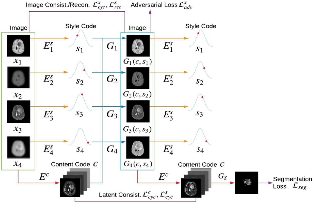
Overview of the proposed n-to-n multi-domain completion and segmentation framework. N = 4 and two domains (x₂, x₄) are missing in this example. Our model contains a unified content encoder E^c (red lines), domain-specific style encoders $E_i^s$ (orange lines) and generators G_i (blue lines), 1 ≤ i ≤ N. A variety of losses are adopted (burgundy lines), i.e., image consistency loss for visible domains ${\mathcal{L}}_{cyc}^x$, latent consistency loss ${\mathcal{L}}_{cyc}^c$ and ${\mathcal{L}}_{cyc}^s$, adversarial loss ${\mathcal{L}}_{adv}^x$ and reconstruction loss ${\mathcal{L}}_{rec}^x$ for the generated images. Furthermore, representational learning framework combines a segmentation generator G_S following the content code for a unified image generation and segmentation.

During the training, our model captures the shared content code c and separate style codes s_i (1 ≤ i ≤ N) through the disentanglement process (denoted as red and orange arrows respectively in Fig. 3) with a random set of input images (in green box). In Fig. 4, we visualize the extracted content codes (randomly selected 8 out of 256 channels) of one BraTS image sample. Various focuses (on different anatomical structures, e.g., tumor, brain, skull) are demonstrated by different channel-wise feature maps. Together with combined individual style code (sampling from a Gaussian distribution $\mathcal{N}\left(\mathbf{0},\mathit{I}\right)$, we only need to train one single ReMIC model to complete the multiple missing domains in the inputs.

Fig. 4.

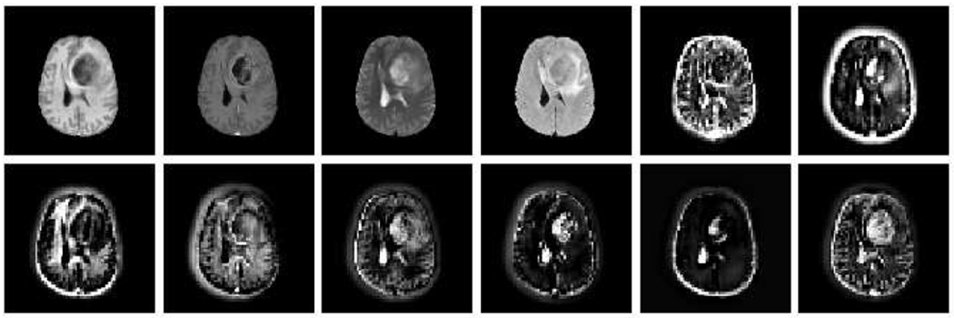
Content codes visualization in BraTS image generation. The first 4 images are ground truth modalities.

In the image generation process (denoted as blue arrows in Fig. 3), our model samples style codes from a prior distribution and integrates with the content code to generate images in N domains through generators G_i (1 ≤ i ≤ N). The generator G_i for each domain generates images in the corresponding domain from the domain-shared content code and the domain-specific style code: $G_i\left(c,s_i\right)={\tilde{x}}_i$.

Additionally, we extend the introduced image completion framework to a more practical scenario, i.e., tackling the missing data problem in image segmentation. Specifically, another branch of segmentation generator G_S is added after content codes to generate the segmentation masks of the input images. Our underlying assumption is that the domain-shared content codes contain essential image structure information for the segmentation task. By simultaneously optimizing the generation loss and segmentation Dice loss (detailed in Section III-B), the model could adaptively learn how to generate missing images to improve the segmentation performance. Please refer to the supplementary (Section Appendix I) for architecture details of content and style encoder, image generator, and segmentation model.

B. Training Loss

In the training of GAN models, the setting of losses is of paramount importance to the final generation results. Our loss functions contain the cycle-consistency loss of images and latent codes, adversarial loss and reconstruction loss on the generated and input images.

1). Image Consistency Loss::

For each sample, the proposed model is able to extract a domain-shared content code and domain-specific style codes respectively from visible domains. Then by recombining the content and style codes, the domain generators are expected to recover the input images. The image consistency loss is defined to constrain the reconstructed images and real images as in the direction of “ Image → Code → Image” in Fig. 3.

$${\mathcal{L}}_{cyc}^{x_i}={\mathbb{E}}_{x_i~p\left(x_i\right)}\left[{\Vert G_i\left(E^c\left(x_1,\mathrm{\cdots },x_N\right),E_i^s\left(x_i\right)\right)-x_i\Vert }_1\right]$$ (1)

where p(x_i) is the data distribution in domain χ_i (1 ≤ i ≤ N). Here, we use ${\mathcal{L}}_1$ loss to strengthen anatomical-structure related generation.

2). Latent Consistency Loss::

The latent consistency loss constrains the learning of both content and style codes before decoding and after encoding in the direction of “Code → Image → Code”.

$${\mathcal{L}}_{cyc}^c={\mathbb{E}}_{c~p\left(c\right),s_i~p\left(s_i\right)}\left[{\Vert E^c\left(G_1\left(c,s_1\right),G_2\left(c,s_2\right),\mathrm{\cdots },G_n\left(c,s_N\right)\right)-c\Vert }_1\right]$$ (2)

$${\mathcal{L}}_{cyc}^{s_i}={\mathbb{E}}_{c~p\left(c\right),s_i~p\left(s_i\right)}\left[{\Vert E_i^s\left(G_i\left(c,s_i\right)\right)-s_i\Vert }_1\right]$$ (3)

where p(s_i) is the prior distribution of style code: $\mathcal{N}\left(\mathbf{0},\mathit{I}\right)$, p(c) is given by c = E^c(x₁, x₂, ⋯, x_N) and x_i ~ p(x_i) (1 ≤ i ≤ N), i.e., the content code is sampled by firstly sampling images from data distribution. Specifically, taking BraTS data as an example, style distribution p(s_i) contains various domain-specific characteristics in each domain, like varied image contrasts. Content distribution p(c) contains various anatomy structure related features among different brain subjects as shown in Fig. 4.

3). Adversarial Loss::

The adversarial learning between generators and discriminators forces the data distribution of the generated images to be close to that of the real images for each domain.

$${\mathcal{L}}_{adv}^{x_i}={\mathbb{E}}_{c~p\left(c\right),s_i~p\left(s_i\right)}\left[\log \left(1-D_i\left(G_i\left(c,s_i\right)\right)\right)\right]+{\mathbb{E}}_{x_i~p\left(x_i\right)}\left[\log D_i\left(x_i\right)\right]$$ (4)

where D_i is the discriminator for domain i to distinguish the generated images ${\tilde{x}}_i$ and real images $x_i\in {\chi }_i$.

4). Reconstruction Loss::

In addition to the feature-level consistency mentioned above to constrain the relationship between the generated images and real images in different domains, we also constrain the pixel-level similarity between generated images and ground truth images in the same domain during training stage, for accurately completing missing domains given visible images of the current subject or scene.

$${\mathcal{L}}_{rec}^{x_i}={\mathbb{E}}_{c~p\left(c\right),s_i~p\left(s_i\right)}\left[{\Vert G_i\left(c,s_i\right)-x_i\Vert }_1\right]$$ (5)

Please note that the image consistency loss in Eq. (1) denotes the encoding and decoding process for only the visible domains. The given input images in the visible domains are encoded as content codes and style codes, which are then directly decoded to recover the input images. The constraints between input images and recovered images are denoted here as image consistency loss. The image reconstruction loss in Eq. (5) denotes the image generation process for all the domains including the missing domains. In the image generation process, the content codes are encoded from given visible domains while the style codes are samples from prior distribution. Thus, this constraint between all the generated images and ground truth images in all the domains is denoted as image reconstruction loss. Without the reconstruction loss in Eq. (5), the whole image generation model is totally unsupervised learning.

5). Segmentation Loss::

In the n-to-n image translation, the model learns a complementary representation of multiple domains, which can further facilitate the high-level tasks. For instance, extracted content code (containing the underlying anatomical structures) may benefit the segmentation of organs and lesions in medical image analysis, vice versa. Therefore, we train a multi-task network for both segmentation and generation. In the proposed framework, we construct a unified generation and segmentation model by adding a segmentation generator G_S following the content code from the completed images as shown in Fig. 3. We utilize Dice loss [38], [39] for accurate segmentation from multiple domain images

$${\mathcal{L}}_{seg}=1-\frac{1}{L}\sum _{l=1}^L\frac{{\sum }_{p}2{\widehat{y}}_p\left(l\right)y_p\left(l\right)}{{\sum }_p{\widehat{y}}_p{\left(l\right)}^2+{\sum }_p{y}_p{\left(l\right)}^2},$$ (6)

where L is the total number of classes, p is the spatial position index in the image, $\widehat{y}\left(l\right)$ is the predicted segmentation probability map for class l from G_S and y(l) is the ground truth segmentation mask for class l. The segmentation loss can be added into the total loss in Eq. 7 for an end-to-end joint learning optionally.

6). Total Loss::

The encoders, generators, discriminators (and segmentor) are jointly trained to optimize the total objective as follows

$$\underset{E^c,E^s,G}{\min }\underset{D}{\max }\mathcal{L}\left(E^c,E_1^s,\mathrm{\cdots },E_N^s,G_1,\mathrm{\cdots },G_N,D_1,\mathrm{\cdots },D_N\right)=\sum _{i=1}^N\left({\lambda }_{cyc}^x{\mathcal{L}}_{cyc}^{x_i}+{\lambda }_{cyc}^s{\mathcal{L}}_{cyc}^{s_i}+{\lambda }_{adv}{\mathcal{L}}_{adv}^{x_i}+{\lambda }_{rec}{\mathcal{L}}_{rec}^{x_i}\right)+{\lambda }_{cyc}^c{\mathcal{L}}_{cyc}^c\left(+{\lambda }_{seg}{\mathcal{L}}_{seg}\right)$$ (7)

where λ_adv, ${\lambda }_{cyc}^x,{\lambda }_{cyc}^c,{\lambda }_{cyc}^s$, λ_rec and λ_seg are hyper-parameters to balance the losses. Please note that the segmentation loss is included in the total training loss only when we train the unified generation and segmentation model for BraTS and ProstateX datasets.

IV. Experiments

To validate the feasibility and generalization of the proposed model, we conduct experiments on two medical image datasets as well as a natural image dataset: BraTS, ProstateX, and RaFD. We firstly demonstrate the advantage of the proposed method in the n-to-n multi-domain image completion task given a random set of visible domains. Moreover, we illustrate that the proposed model (a variation with two branches of image translation and segmentation) provides an efficient solution to multi-domain segmentation with missing-domain inputs.

A. BraTS:

The Multimodal Brain Tumor Segmentation Challenge (BraTS) 2018 [1], [40], [41] provides multi-modal brain MRI with four modalities: a) native (T1), b) post-contrast T1-weighted (T1Gd), c) T2-weighted (T2), and d) T2 Fluid Attenuated Inversion Recovery (FLAIR). Following CollaGAN [42], 218 and 28 subjects are randomly selected for training and testing. A set of 2D slices is extracted from 3D volumes for four modalities respectively. In total, the training and testing sets contain 40,148 and 5,340 images. We resize the images of size 240 × 240 to 256 × 256. Three categories are labeled for brain tumor segmentation, i.e., enhancing tumor (ET), tumor core (TC), and whole tumor (WT).

B. ProstateX:

The ProstateX dataset [43] contains multi-parametric prostate MR scans for 98 subjects. Each sample contains three modalities : 1) T2-weighted (T2), 2) Apparent Diffusion Coefficient (ADC), 3) high b-value DWI images (HighB). We randomly split it into 78 and 20 subjects for training and testing respectively. By extracting 2D slices from 3D volumes, the training and testing sets contain 3,540 and 840 images in total. Images of 384 × 384 are resized to 256 × 256. Prostate regions are manually labeled as the whole prostate (WP) by board-certificated radiologists.

C. RaFD:

The Radboud Faces Database (RaFD) [44] contains eight facial expressions collected from 67 participants: neutral, angry, contemptuous, disgusted, fearful, happy, sad, and surprised. Following StarGAN [11], we adopt images from three camera angles (45°, 90°, 135°) with three gaze directions (left, frontal, right), and obtain 4,824 images in total. The data is randomly split to training set of 54 participants (3,888 images) and testing set of 13 participants (936 images). We crop the image with the face in the center and then resize to 128 × 128.

In all experiments, we set λ_adv = 1, ${\lambda }_{cyc}^x=10$, ${\lambda }_{cyc}^c=1$, ${\lambda }_{cyc}^s=1$, λ_rec = 20, and λ_seg = 1 if ${\mathcal{L}}_{seg}$ is included in Eq. 7. The adversarial loss λ_adv and consistency loss ${\lambda }_{cyc}^x,{\lambda }_{cyc}^c,{\lambda }_{cyc}^s$ follow the same loss weights choices as in [19] which reported the necessity of the consistency losses in its ablative study. In the following, we will demonstrate ablative studies on the reconstruction and segmentation loss.

V. Results

A. Results of Multi-Domain Image Completion

For comparison purpose, we firstly assume there are only one missing domain for each data sample. In training, the one missing domain is randomly distributed among all the N domains. During testing, at a time, we fix the one missing domain in inputs and evaluate the generation outputs only on that missing modality, whose results are demonstrated in one column (modality) of Table I, II. Multiple metrics are used to measure the similarity between the generated and teh target images, i.e., normalized root mean-squared error (NRMSE), mean structural similarity index (SSIM), and peak-signal-noise ratio (PSNR). We compare our results with previous methods on all three datasets. The results of the proposed method (“ReMIC”), ReMIC without reconstruction loss (“ReMIC w/o Recon”) are reported.

TABLE I.

BraTS and Prostate multi-domain image completion results.

(a) BraTS
Methods	T1	TIGd	T2	FLAIR
	NRMSE(↓) / SSIM(↑) / PSNR(↑)	NRMSE(↓) / SSIM(↑) / PSNR(↑)	NRMSE(↓) / SSIM(↑) / PSNR(↑)	NRMSE(↓) / SSIM(↑) / PSNR(↑)
MUNIT [19]	0.3709 / 0.9076 / 23.2385	0.2827 / 0.9221 / 27.3836	0.4073 / 0.8757 / 22.8936	0.4576 / 0.8702 / 21.5568
StarGAN [11]	0.3233 / 0.9282 / 24.2840	0.2718 / 0.9367 / 27.6901	0.5002 / 0.8464 / 21.3614	0.4642 / 0.8855 / 22.0483
CollaGAN [13]	0.4800 / 0.8954 / 21.2803	0.4910 / 0.8706 / 22.9042	0.5310 / 0.8886 / 21.2163	0.4231 / 0.8635 / 22.4188
ReMIC w/o Recon	0.3366 / 0.9401 / 24.5787	0.2398 / 0.9435 / 28.8571	0.3865 / 0.9011 / 23.4876	0.3650 / 0.8978 / 23.5918
ReMIC	0.2008 / 0.9618 / 28.5508	0.2375 / 0.9521 / 29.1628	0.2481 / 0.9457 / 27.4829	0.2469 / 0.9367 / 27.1540
ReMIC-Random(k=1)	0.2263 / 0.9603 / 27.5198	0.2118 / 0.9600 / 30.5945	0.2566 / 0.9475 / 27.7646	0.2742 / 0.9399 / 26.8257
Re MIC-Random(k=2)	0.1665 / 0.9751 / 30.8579	0.1697 / 0.9730 / 32.7615	0.1992 / 0.9659 / 30.3789	0.2027 / 0.9591 / 29.7351
ReMIC-Random(k=3)	0.1274 / 0.9836 / 33.2458	0.1405 / 0.9812 / 34.3967	0.1511 / 0.9788 / 32.6743	0.1586 / 0.9724 / 31.8967

(b) ProstateX
Methods	T2	ADC	HighB
	NRMSE(↓) / SSIM(↑) / PSNR(↑)	NRMSE(↓) / SSIM(↑) / PSNR(↑)	NRMSE(↓) / SSIM(↓) / PSNR(↓)
MUNIT [19]	0.6904 / 0.4428 / 15.6308	0.9208 / 0.4297 / 13.8983	0.9325 / 0.5383 / 16.9616
StarGAN [11]	0.6638 / 0.4229 / 15.9468	0.9157 / 0.3665 / 13.8014	0.9188 / 0.4350 / 17.1168
CollaGAN [13]	0.8070 / 0.2667 / 14.2640	0.7621 / 0.4875 / 15.4242	0.7722 / 0.6824 / 18.6481
ReMIC w/o Recon	0.8567 / 0.3330 / 13.6738	0.7289 / 0.5377 / 15.7083	0.8469 / 0.7818 / 17.8987
ReMIC	0.4908 / 0.5427 / 18.6200	0.2179 / 0.9232 / 26.6150	0.3894 / 0.9150 / 24.7927
ReMIC-Random(k=1)	0.3786 / 0.6569 / 22.5314	0.2959 / 0.8256 / 26.9485	0.4091 / 0.8439 / 27.7499
ReMIC-Random(k=2)	0.2340 / 0.8166 / 27.0598	0.1224 / 0.9664 / 33.2475	0.1958 / 0.9587 / 34.4775

TABLE II.

RaFD multi-domain image completion results.

Methods	Neutral	Angry	Contemptuous	Disgusted
	NRMSE(↓) / SSIM(↑) / PSNR(↑)	NRMSE(↓) / SSIM(↑) / PSNR(↑)	NRMSE(↓) / SSIM(↑) / PSNR(↑)	NRMSE(↓) / SSIM(↑) / PSNR(↑)
MUNIT [19]	0.1589 / 0.8177 / 19.8469	0.1637 / 0.8156 / 19.7303	0.1518 / 0.8319 / 20.2793	0.1563 / 0.8114 / 19.9362
StarGAN [11]	0.1726 / 0.8206 / 19.2725	0.1722 / 0.8245 / 19.4336	0.1459 / 0.8506 / 20.7605	0.1556 / 0.8243 / 20.0036
CollaGAN [13]	0.1867 / 0.7934 / 18.3691	0.1761 / 0.7736 / 18.8678	0.1856 / 0.7928 / 18.4040	0.1823 / 0.7812 / 18.5160
ReMIC w/o Recon	0.1215 / 0.8776 / 22.2963	0.1335 / 0.8556 / 21.4615	0.1192 / 0.8740 / 22.4073	0.1206 / 0.8559 / 22.1819
ReMIC	0.1225 / 0.8794 / 22.2679	0.1290 / 0.8598 / 21.7570	0.1217 / 0.8725 / 22.2414	0.1177 / 0.8668 / 22.4135
ReMIC-Random(k=1)	0.1496 / 0.8317 / 20.7821	0.1413 / 0.8368 / 21.5096	0.1407 / 0.8348 / 21.2486	0.1394 / 0.8352 / 21.4443
Re MIC-Random(k=4)	0.0990 / 0.9014 / 24.7746	0.0988 / 0.8964 / 24.8327	0.0913 / 0.9048 / 25.2826	0.0969 / 0.8934 / 24.8231
ReMIC-Random(k=7)	0.0756 / 0.9280 / 26.6861	0.0679 / 0.9332 / 27.4557	0.0665 / 0.9346 / 27.5942	0.0675 / 0.9308 / 27.3955
Methods	Fearful	Happy	Sad	Surprised
	NRMSE(↓) / SSIM(↑) / PSNR(↑)	NRMSE(↓) / SSIM(↓) / PSNR(↓)	NRMSE(↓) / SSIM(↑) / PSNR(↑)	NRMS(↓) / SSIM(↑) / PSNR(↑)
MUNIT [19]	0.1714 / 0.7792 / 19.1714	0.1623 / 0.8073 / 19.7709	0.1677 / 0.7998 / 19.3867	0.1694 / 0.7884 / 19.3867
StarGAN [11]	0.1685 / 0.7943 / 19.3516	0.1522 / 0.8288 / 20.4397	0.1620 / 0.8227 / 19.7368	0.1634 / 0.7974 / 19.6744
CollaGAN [13]	0.1907 / 0.7442 / 18.1518	0.1829 / 0.7601 / 18.5503	0.1783 / 0.7766 / 18.7450	0.1888 / 0.7495 / 18.2169
ReMIC w/o Recon	0.1321 / 0.8384 / 21.4604	0.1399 / 0.8332 / 20.9334	0.1284 / 0.8597 / 21.7430	0.1333 / 0.8347 / 21.3782
ReMIC	0.1316 / 0.8395 / 21.5295	0.1383 / 0.8406/ 21.0465	0.1301 / 0.8581 / 21.6384	0.1276 / 0.8484 / 21.7793
ReMIC-Random(k=1)	0.1479 / 0.8132 / 21.0039	0.1567 / 0.8121 / 20.3798	0.1491 / 0.8244 / 20.6888	0.1434 / 0.8218 / 21.2411
Re MIC-Random(k=4)	0.1043 / 0.8769 / 24.2623	0.1065 / 0.8852 / 23.9813	0.0960 / 0.8971 / 24.9114	0.1022 / 0.8835 / 24.2613
ReMIC-Random(k=7)	0.0769 / 0.9209 / 26.5362	0.0794 / 0.9200 / 26.1515	0.0729 / 0.9291 / 26.8993	0.0735 / 0.9248 / 26.7651

Moreover, we investigate a more practical scenario when there are more than one missing domains and show that our proposed method is capable to handle a general random n-to-n image completion. In this setting, we assume the set of missing domains in training data is randomly distributed, i.e. each training data has k randomly selected visible domains where k ≥ 1. During testing, we fix the number of visible domains k(k ∈ {1, …, N−1}) while these k available domains are also randomly distributed among N domains. We evaluate all the N generated images in outputs, showing results in all columns (modalities) of Table I, II. “ReMIC-Random(k = *)” denotes evaluation on the test set with k random visible domains or N – k random missing domains. Note that by leveraging the unified content code and sampling the style code for each domain respectively, the proposed model could handle any number of missing domains, which is more general and flexible for the random k-to-n image completion as shown in Fig. 1(d). We compare our model with following methods: MUNIT [19] conducts 1-to-1 image translation between two domains through representational disentanglement as shown in Fig. 1(a). In RaFD experiments, we train and test MUNIT models between any pair of two domains. Without loss of generality, we use “neural” image to generate all the other domains by following StarGAN setting, and “angry” image is used to generate “neural” image. In BraTS , the typical modality “T1” is used to generate other domains while “T1” is generated from “TIGd”. Similarly, “T2” is used to generate other domains in ProstateX while it is generated from “ADC”. StarGAN [11] adopts a mask vector to generate image in the specified target domain. In this way, different target domains could be generated from one source domain in multiple inference passes. This is actually a 1-to-n image translation as in Fig. 1(b). Since only one domain can be used as input in StarGAN, we use the same domain pair match as MUNIT, following the same setting in [11].

CollaGAN [13], [42] carries out the n-to-1 image translation in Fig. 1(c), where multiple source domains collaboratively generate one target domain which is assumed missing in inputs. But it does not deal with multiple missing domains. In CollaGAN experiments, we use the same domain generation setting as ours, i.e., fix one missing domain in inputs and generate from all the other domains.

1). Results of medical image generation:

Fig. 5 and Fig. 7 show the results of image completion (modalities in rows) on BraTS and ProstateX data in comparison to others [11], [13], [19] (methods in columns). Each cell illustrates the generated image when the current modality is missing in inputs. The corresponding quantitative results averaged across all testing data are shown in Table I. In comparison, our model generates better results in meaningful details, e.g., a more accurate outstanding tumor region in BraTS and prostate regions are better-preserved in ProstateX. This is achieved by learning a better complementary content code from multiple input domains through factorized latent space in our method, which is essential in preserving the anatomical structures in medical images. Furthermore, we illustrate the generation results when multiple modalities are missing in BraTS and ProstateX dataset. We show the results in the rows of Fig. 6 and Fig. 8, where images are generated when only the first k modalities (from left to right) are given in the inputs (1 ≤ k ≤ N − 1). The averaged quantitative results for random k-to-n image generation are denoted as “ReMIC-Random(k = *)” in Table I.

Fig. 5.

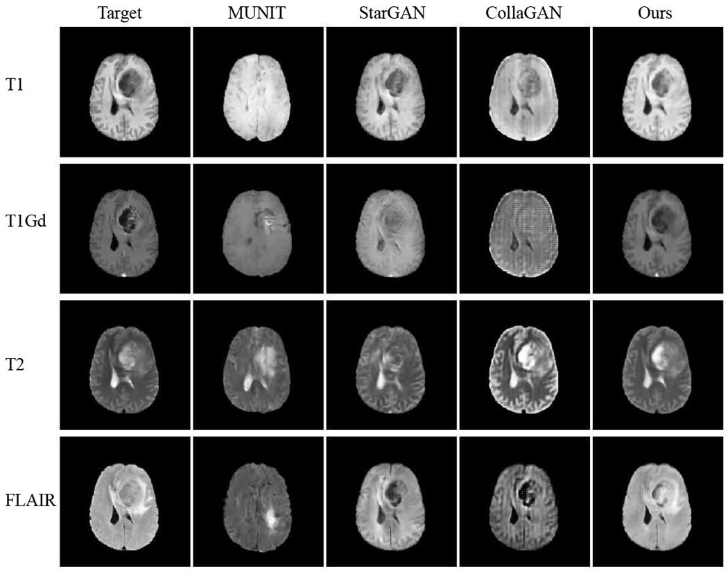
BraTS image generation results with a single missing modality. Rows: 4 modalities. Columns: compared methods.

Fig. 7.

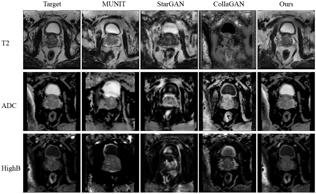
ProstateX image generation results. Rows: 3 modalities. Columns: compared methods.

Fig. 6.

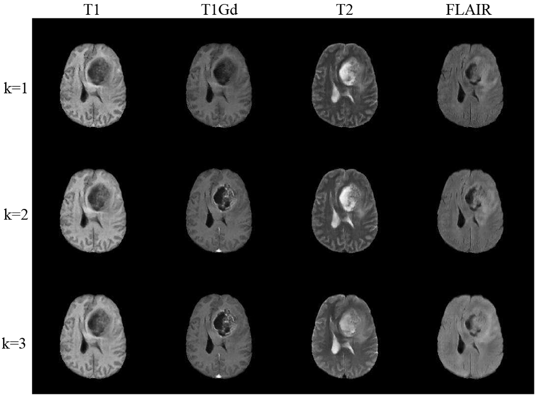
BraTS image generation results with multiple missing modalities (in columns). Ground truth image for each modality is shown in “Target” column of Fig. 5. Rows: the first k domains (from left to right) are given in inputs (1 ≤ k ≤ 3)

Fig. 8.

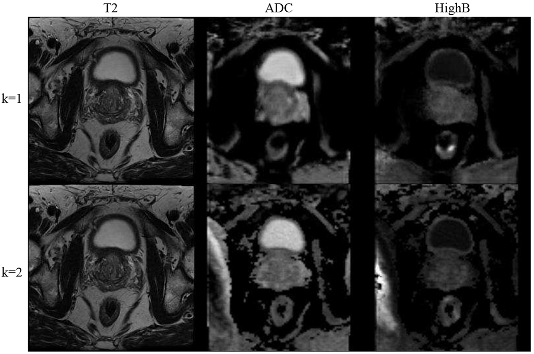
ProstateX image generation results with multiple missing modalities (in columns). Ground truth image for each modality is shown in “Target” column of Fig. 7. Rows: the first k domains (from left to right) are given in inputs (1 ≤ k ≤ 2).

2). Results of facial expression image generation:

Fig. 9 shows the result of facial expression image completion for RaFD dataset. In each column, we show the target and generated images of each domain (facial expression), where we assume the current target domain is missing in the inputs at a time and needs to be generated using the rest N − 1 available domains. Compared with MUNIT and StarGAN results, our method could generate missing images with a better quality, especially in generating details like teeth, mouth and eyes. This benefits from that our method can incorporate complementary information from multiple available domains, while MUNIT and StarGAN can adopt only one domain as input. For example, in the generation of “happy” and “disgusted” expressions, either MUNIT nor StarGAN could generate a good teeth and mouth region, since their source domain “neutral” does not contain the teeth. Compared with CollaGAN, our method could generate images with a better content due to the explicit disentangled representational learning in feature level instead of the implicit cycle-consistency constraints only in pixel level. Moreover, Fig. 10 shows the results of multiple missing domains. Each row shows the generated images in each of 8 domains, when the first k domains (from left to right) are given in inputs (1 ≤ k ≤ 7). The superior performance could also be observed in the NRMSE, and SSIM and PSNR evaluation metrics averaged across all testing samples as reported in Table II with all the eight expression domains. Please refer to the supplementary (Section Appendix II) for extended results and ablative study of multi-domain image completion.

Fig. 9.

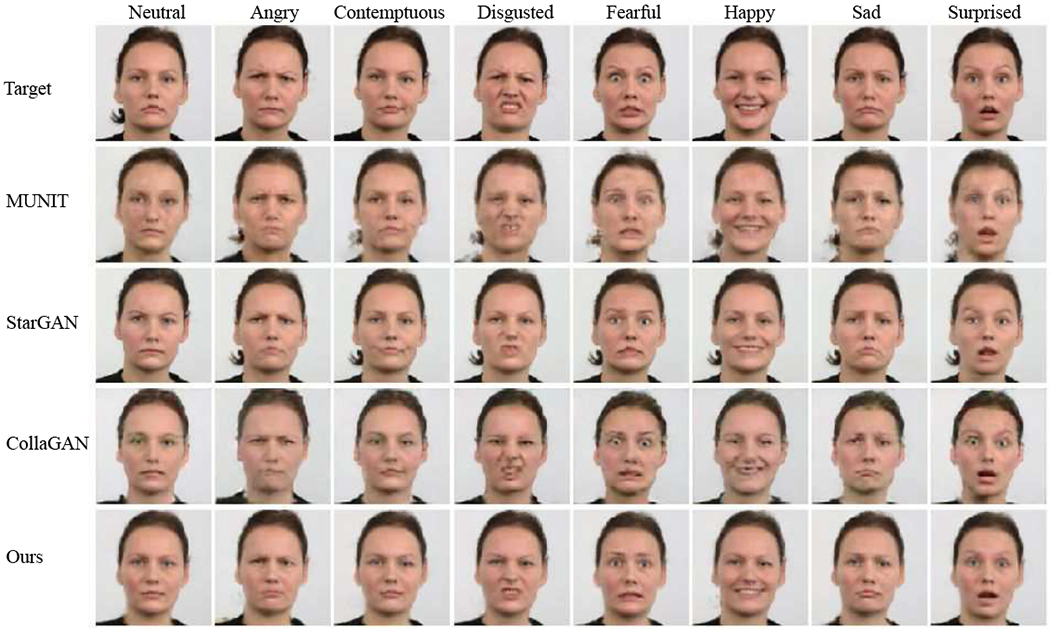
RaFD image generation results with a single missing modality. Columns: 8 facial expressions. Rows: compared methods.

Fig. 10.

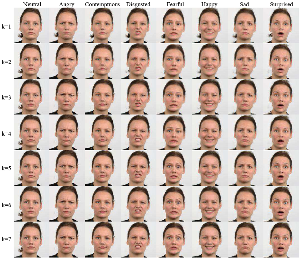
RaFD image generation results with multiple missing modalities (in columns). Ground truth image for each modality is shown in “Target” row of Fig. 9. Rows: the first k domains (from left to right) are given in inputs (1 ≤ k ≤ 7).

B. Results of Missing-Domain Segmentation

Based on the missing-domain image completion, we demonstrate that our proposed method could go beyond image generation to solve the missing-domain image segmentation. specifically, our model learns factorized representations by disentangling latent space, which could be efficiently leveraged for high-level segmentation task. As shown in Fig. 3, a segmentation branch is added using the learned content code to generate segmentation prediction. We evaluate the segmentation performance with Dice coefficient on both BraTs and ProstateX datasets as shown in Table III. Please note that we show the average Dice coefficient across three categories for BraTS dataset: enhancing tumor (ET), tumor core (TC), and whole tumor (WT). (details of per-category results in supplementary.)

TABLE III.

Missing-domain segmentation. (Dice scores are reported.)

Methods	BraTS				ProstateX
	T1	T1Gd	T2	FLAIR	T2	ADC	HighB
Oracle+All	0.822				0.908
Oracel+Zero padding	0.651	0.473	0.707	0.454	0.528	0.243	0.775
Oracle+Average imputation	0.763	0.596	0.756	0.671	0.221	0.692	0.685
Oracle+Nearest neighbor	0.769	0.540	0.724	0.606	0.759	0.850	0.854
Oracle+MUNIT	0.783	0.537	0.782	0.492	0.783	0.708	0.858
Oracle+StarGAN	0.799	0.553	0.746	0.613	0.632	0.653	0.832
Oracle+CollaGAN	0.753	0.564	0.798	0.674	0.472	0.760	0.842
Oracle+ReMIC	0.789	0.655	0.805	0.765	0.871	0.898	0.891
ReMIC+Seg	0.806	0.674	0.822	0.771	0.872	0.909	0.905
ReMIC+Joint	0.828	0.693	0.828	0.791	0.867	0.904	0.904

We train a fully supervised 2D U-shaped segmentation network (a U-Net variation [45]) without missing images as the “Oracle”. “Oracle+*” means that the results are computed by predicting the multi-modal segmentation with the missing images generated or imputed from the “*” method using the pretrained “Oracle” model. “All” represents the full testing data without any missing domains. “ReMIC+Seg” stands for using separate content encoders for image generation and segmentation tasks in our proposed unified framework, while “ReMIC+Joint” indicates sharing the weights of content encoder for the two tasks. Please note that for each column in Table III, we report the multi-modal segmentation results when the current modality is missing and synthesized while the other modalities are available. For the results on both datasets, our proposed unified framework with joint training of image generation and segmentation could achieve the best segmentation performance in comparison to other imputation or generation methods. This indicates that the joint training model can generate better images in missing domains that adaptively extract more useful information for the downstream task like segmentation. Moreover, it even obtains comparable results as “Oracle” model when some modalities are missing. This indicates that the learned content codes indeed embed and extract efficient anatomical structures for image representation.

In our experiments, we choose the widely used U-shaped segmentation network [45] as the backbone for segmentation generator G_S. Here, we focus on showing how the proposed method could benefit the segmentation when missing domains exist and the segmentation backbone is fixed. But our method can also be easily generalized to other segmentation models with a similar methodology. Please refer to the supplementary (Section Appendix III) for extended results and ablative study of missing-domain image segmentation.

VI. Discussion

In the paper, we assume the imaging objects have generally the same structure (that is, after alignment) across different domains. These shared structures of the same subject are the content code assumed in the paper, while the other domain-specific features are related to the style encoding such as the expression-related landmark variations or image contrasts in different domains. There may be some limitations with such an assumption, for example, the hairs that may not be aligned as the example shown in Fig. 10, which rely on the available source domains. But in the applications presented in the paper, we focus more on preserving the overall structures, that is, the outline and relative location of tumor regions and consistent appearance of facial landmarks.

From experiments, we observe an interesting finding that the reconstruction loss plays a different effect for medical and natural images. For natural images such as facial images in the RaFD, comparing the results of “ReMIC w/o Recon” and “ReMIC” in Table 2, we can see that there is not a big difference when adding reconstruction loss. This shows that our method can learn image generation in a totally unsupervised way through feature disentanglement. For medical images, we see that although “ReMIC w/o Recon” already outperforms the other methods such as MUNIT, StarGAN and CollaGAN under the same setting, the reconstruction loss brings further advantage to generate better image quality. We think this is because the domain translation for medical images is even more challenging due to the contrast-specific information from different modalities.

In the paper, although the unified model adopts a U-Net shape segmentor and experiments on brain tumor segmentation and prostate segmentation, please note that the segmentation model in the framework are exchangeable. Thus, the insight of the method for random n-to-n mapping can be deployed to any other segmentation models and generalized to other downstream tasks such as segmentation for other organs [32–34].

In practical scenarios, the missing data problems are very common. For example, clinical scanning protocol for the same disease may differ among institutes, e.g., perfusion weighted images may be optional, and different B-value images may be acquired for computing ADC maps. Then, this random missing input data problem will affect both model development and deployment across institutes. Motivated by this, we propose a general solution to this practical problem by multi-domain image completion. To validate the proposed method, we design the corresponding experiments on three datasets with the missing input data scenarios, and the results validate the feasibility of the proposed method for image completion. Furthermore, we deploy the model for the segmentation task to show how this method can be useful in real applications. Thus, we think the proposed method potentially provides a general solution to deal with such scenarios in practice.

VII. Conclusion

In this work, we propose a general framework for multi-domain image completion, given that one or more input domains are missing. The proposed model learns shared content and domain-specific style encoding across multiple domains. We show the proposed image completion approach can be well generalized to both natural and medical images. our framework is further extended to a unified image generation and segmentation framework to tackle a practical problem of missing-domain segmentation. Experiments on three datasets demonstrate the proposed method consistently achieves better performance than several previous approaches on both multi-domain image completion and segmentation with random missing domains. Furthermore, although the work is extensively evaluated for brain and prostate multi-contrast MR image completion, experiments on real-world and large scale clinical experiments are required before clinical usage. In the next step, it is expected to conduct large scale clinical experiments to validate the effectiveness coping with the data discrepancy issue widely existing in the real world. Concluding, the proposed method paves the way for many potential medical image applications with the common missing data problems.

References

- [1].Menze BH et al. , “The multimodal brain tumor image segmentation benchmark (brats),” IEEE transactions on medical imaging, vol. 34, no. 10, pp. 1993–2024, 2014. [DOI] [PMC free article] [PubMed] [Google Scholar]
- [2].Zheng L, Shen L, Tian L, Wang S, Wang J, and Tian Q, “Scalable person re-identification: A benchmark,” in Proceedings of the IEEE international conference on computer vision, 2015, pp. 1116–1124. [Google Scholar]
- [3].Zheng Z, Yang X, Yu Z, Zheng L, Yang Y, and Kautz J, “Joint discriminative and generative learning for person re-identification,” in Proceedings of the IEEE Conference on Computer Vision and Pattern Recognition, 2019, pp. 2138–2147. [Google Scholar]
- [4].Goodfellow I et al. , “Generative adversarial nets,” in Advances in neural information processing systems, 2014, pp. 2672–2680. [Google Scholar]
- [5].Mirza M and Osindero S, “Conditional generative adversarial nets,” arXiv preprint arXiv:1411.1784, 2014. [Google Scholar]
- [6].Isola P, Zhu J-Y, Zhou T, and Efros AA, “Image-to-image translation with conditional adversarial networks,” in Proceedings of the IEEE conference on computer vision and pattern recognition, 2017, pp. 1125–1134. [Google Scholar]
- [7].Zhu J-Y, Park T, Isola P, and Efros AA, “Unpaired image-to-image translation using cycle-consistent adversarial networks,” in Proceedings of the IEEE international conference on computer vision, 2017, pp. 2223–2232. [Google Scholar]
- [8].Zhu J-Y et al. , “Toward multimodal image-to-image translation,” in Advances in Neural Information Processing Systems, 2017. [Google Scholar]
- [9].Kim T, Cha M, Kim H, Lee JK, and Kim J, “Learning to discover cross-domain relations with generative adversarial networks,” in Proceedings of the 34th International Conference on Machine Learning-Volume 70. JMLR.org, 2017, pp. 1857–1865. [Google Scholar]
- [10].Liu M-Y, Breuel T, and Kautz J, “Unsupervised image-to-image translation networks,” in Advances in neural information processing systems, 2017, pp. 700–708. [Google Scholar]
- [11].Choi Y, Choi M, Kim M, Ha J-W, Kim S, and Choo J, “Stargan: Unified generative adversarial networks for multi-domain image-to-image translation,” in Proceedings of the IEEE Conference on Computer Vision and Pattern Recognition, 2018, pp. 8789–8797. [Google Scholar]
- [12].Yoon J, Jordon J, and van der Schaar M, “Radialgan: Leveraging multiple datasets to improve target-specific predictive models using generative adversarial networks,” arXiv preprint arXiv:1802.06403, 2018. [Google Scholar]
- [13].Lee D, Kim J, Moon W-J, and Ye JC, “Collagan: Collaborative gan for missing image data imputation,” in Proceedings of the IEEE Conference on Computer Vision and Pattern Recognition, 2019, pp. 2487–2496. [Google Scholar]
- [14].Zhang Z, Yang L, and Zheng Y, “Translating and segmenting multimodal medical volumes with cycle-and shape-consistency generative adversarial network,” in Proceedings of the IEEE Conference on Computer Vision and Pattern Recognition, 2018, pp. 9242–9251. [Google Scholar]
- [15].Dar SU, Yurt M, Karacan L, Erdem A, Erdem E, and Cukur T, “Image synthesis in multi-contrast mri with conditional generative adversarial networks,” IEEE transactions on medical imaging, 2019. [DOI] [PubMed] [Google Scholar]
- [16].Sharma A and Hamarneh G, “Missing mri pulse sequence synthesis using multi-modal generative adversarial network,” IEEE transactions on medical imaging, 2019. [DOI] [PubMed] [Google Scholar]
- [17].Chen X, Duan Y, Houthooft R, Schulman J, Sutskever I, and Abbeel P, “Infogan: Interpretable representation learning by information maximizing generative adversarial nets,” in Advances in neural information processing systems, 2016, pp. 2172–2180. [Google Scholar]
- [18].Higgins I et al. , “beta-vae: Learning basic visual concepts with a constrained variational framework.” ICLR, vol. 2, no. 5, p. 6, 2017. [Google Scholar]
- [19].Huang X, Liu M-Y, Belongie S, and Kautz J, “Multimodal unsupervised image-to-image translation,” in Proceedings of the European Conference on Computer Vision (ECCV), 2018, pp. 172–189. [Google Scholar]
- [20].Lee H-Y, Tseng H-Y, Huang J-B, Singh MK, and Yang M-H, “Diverse image-to-image translation via disentangled representations,” in European Conference on Computer Vision, 2018. [Google Scholar]
- [21].Lee H-Y et al. , “Drit++: Diverse image-to-image translation via disentangled representations,” arXiv preprint arXiv:1905.01270, 2019. [Google Scholar]
- [22].Lin J, Chen Z, Xia Y, Liu S, Qin T, and Luo J, “Exploring explicit domain supervision for latent space disentanglement in unpaired image-to-image translation,” IEEE transactions on pattern analysis and machine intelligence, 2019. [DOI] [PubMed] [Google Scholar]
- [23].Liu Y-C, Yeh Y-Y, Fu T-C, Wang S-D, Chiu W-C, and Frank Wang Y-C, “Detach and adapt: Learning cross-domain disentangled deep representation,” in Proceedings of the IEEE Conference on Computer Vision and Pattern Recognition, 2018, pp. 8867–8876. [Google Scholar]
- [24].Liu AH, Liu Y-C, Yeh Y-Y, and Wang Y-CF, “A unified feature disentangler for multi-domain image translation and manipulation,” in Advances in Neural Information Processing Systems, 2018, pp. 2590–2599. [Google Scholar]
- [25].Huo Y, Xu Z, Bao S, Assad A, Abramson RG, and Landman BA, “Adversarial synthesis learning enables segmentation without target modality ground truth,” in 2018 IEEE 15th International Symposium on Biomedical Imaging (ISBI 2018). IEEE, 2018, pp. 1217–1220. [Google Scholar]
- [26].Iglesias JE, Konukoglu E, Zikic D, Glocker B, Van Leemput K, and Fischl B, “Is synthesizing mri contrast useful for inter-modality analysis?” in International Conference on Medical Image Computing and Computer-Assisted Intervention. Springer, 2013, pp. 631–638. [DOI] [PMC free article] [PubMed] [Google Scholar]
- [27].Shrivastava A, Pfister T, Tuzel O, Susskind J, Wang W, and Webb R, “Learning from simulated and unsupervised images through adversarial training,” in Proceedings of the IEEE conference on computer vision and pattern recognition, 2017, pp. 2107–2116. [Google Scholar]
- [28].Costa P et al. , “Towards adversarial retinal image synthesis,” arXiv preprint arXiv:1701.08974, 2017. [Google Scholar]
- [29].Kamnitsas K et al. , “Unsupervised domain adaptation in brain lesion segmentation with adversarial networks,” in International conference on information processing in medical imaging. Springer, 2017, pp. 597–609. [Google Scholar]
- [30].Nie D et al. , “Medical image synthesis with context-aware generative adversarial networks,” in International Conference on Medical Image Computing and Computer-Assisted Intervention. Springer, 2017, pp. 417–425. [DOI] [PMC free article] [PubMed] [Google Scholar]
- [31].Zhu W, Xiang X, Tran TD, Hager GD, and Xie X, “Adversarial deep structured nets for mass segmentation from mammograms,” in 2018 IEEE 15th International Symposium on Biomedical Imaging (ISBI 2018). IEEE, 2018, pp. 847–850. [Google Scholar]
- [32].Yang J, Dvornek NC, Zhang F, Chapiro J, Lin M, and Duncan JS, “Unsupervised domain adaptation via disentangled representations: Application to cross-modality liver segmentation,” in International Conference on Medical Image Computing and Computer-Assisted Intervention. Springer, 2019, pp. 255–263. [DOI] [PMC free article] [PubMed] [Google Scholar]
- [33].Chen X, Lian C, Wang L, Deng H, Fung SH, Nie D, Thung K-H, Yap P-T, Gateno J, Xia JJ et al. , “One-shot generative adversarial learning for mri segmentation of craniomaxillofacial bony structures,” IEEE Transactions on Medical Imaging, vol. 39, no. 3, pp. 787–796, 2019. [DOI] [PMC free article] [PubMed] [Google Scholar]
- [34].Huo Y, Xu Z, Moon H, Bao S, Assad A, Moyo TK, Savona MR, Abramson RG, and Landman BA, “Synseg-net: Synthetic segmentation without target modality ground truth,” IEEE transactions on medical imaging, vol. 38, no. 4, pp. 1016–1025, 2018. [DOI] [PMC free article] [PubMed] [Google Scholar]
- [35].Van Nguyen H, Zhou K, and Vemulapalli R, “Cross-domain synthesis of medical images using efficient location-sensitive deep network,” in International Conference on Medical Image Computing and Computer-Assisted Intervention. Springer, 2015, pp. 677–684. [Google Scholar]
- [36].Havaei M, Guizard N, Chapados N, and Bengio Y, “Hemis: Hetero-modal image segmentation,” in International Conference on Medical Image Computing and Computer-Assisted Intervention. Springer, 2016, pp. 469–477. [Google Scholar]
- [37].Chartsias A, Joyce T, Giuffrida MV, and Tsaftaris SA, “Multimodal mr synthesis via modality-invariant latent representation,” IEEE transactions on medical imaging, vol. 37, no. 3, pp. 803–814, 2017. [DOI] [PMC free article] [PubMed] [Google Scholar]
- [38].Milletari F, Navab N, and Ahmadi S-A, “V-net: Fully convolutional neural networks for volumetric medical image segmentation,” in 2016 Fourth International Conference on 3D Vision (3DV). IEEE, 2016, pp. 565–571. [Google Scholar]
- [39].Salehi SSM, Erdogmus D, and Gholipour A, “Tversky loss function for image segmentation using 3d fully convolutional deep networks,” in International Workshop on Machine Learning in Medical Imaging. Springer, 2017, pp. 379–387. [Google Scholar]
- [40].Bakas S et al. , “Advancing the cancer genome atlas glioma mri collections with expert segmentation labels and radiomic features,” Scientific data, vol. 4, p. 170117, 2017. [DOI] [PMC free article] [PubMed] [Google Scholar]
- [41].Bakas S, Reyes M et al. , “Identifying the best machine learning algorithms for brain tumor segmentation, progression assessment, and overall survival prediction in the brats challenge,” arXiv preprint arXiv:1811.02629, 2018. [Google Scholar]
- [42].Lee D, Moon W-J, and Ye JC, “Which contrast does matter? towards a deep understanding of mr contrast using collaborative gan,” arXiv preprint arXiv:1905.04105, 2019. [Google Scholar]
- [43].Litjens G, Debats O, Barentsz J, Karssemeijer N, and Huisman H, “Computer-aided detection of prostate cancer in mri,” IEEE transactions on medical imaging, vol. 33, no. 5, pp. 1083–1092, 2014. [DOI] [PubMed] [Google Scholar]
- [44].Langner O, Dotsch R, Bijlstra G, Wigboldus DH, Hawk ST, and Van Knippenberg A, “Presentation and validation of the radboud faces database,” Cognition and emotion, vol. 24, no. 8, pp. 1377–1388, 2010. [Google Scholar]
- [45].Ronneberger O, Fischer P, and Brox T, “U-net: Convolutional networks for biomedical image segmentation,” in International Conference on Medical image computing and computer-assisted intervention. Springer, 2015, pp. 234–241. [Google Scholar]
Associated Data
This section collects any data citations, data availability statements, or supplementary materials included in this article.