Application of reinforcement learning for effective vaccination strategies of coronavirus disease 2019 (COVID-19)

Abstract

Since December 2019, the new coronavirus has raged in China and subsequently all over the world. From the first days, researchers have tried to discover vaccines to combat the epidemic. Several vaccines are now available as a result of the contributions of those researchers. As a matter of fact, the available vaccines should be used in effective and efficient manners to put the pandemic to an end. Hence, a major problem now is how to efficiently distribute these available vaccines among various components of the population. Using mathematical modeling and reinforcement learning control approaches, the present article aims to address this issue. To this end, a deterministic Susceptible-Exposed-Infectious-Recovered-type model with additional vaccine components is proposed. The proposed mathematical model can be used to simulate the consequences of vaccination policies. Then, the suppression of the outbreak is taken to account. The main objective is to reduce the effects of Covid-19 and its domino effects which stem from its spreading and progression. Therefore, to reach optimal policies, reinforcement learning optimal control is implemented, and four different optimal strategies are extracted. Demonstrating the efficacy of the proposed methods, finally, numerical simulations are presented.

Introduction

Since the first reported case of coronavirus disease 2019 (COVID-19) in early December 2019 in China, it has resulted in an ongoing crisis that unprecedentedly spreads all around the world [1–4]. Acute respiratory syndrome can occur in patients with serious illness, leading to multiple organ failures and death in some cases. [5, 6]. It has been established that the present pandemic's spread rate is much higher than similar previously reported epidemics in 2003 and 2012, namely SARS coronavirus (SARS-CoV) and MERS coronavirus (MERS-CoV). Until now, the epidemic crisis has resulted in a growing number of deaths all over the globe [7, 8].

Mathematical simulations have long been used to obtain insight into the mechanisms of disease transmission [9–22]. The essence of modeling lies in defining a set of equations that mimic the system's spread or dynamic in reality [23, 24]. From the beginning of the current epidemy, the mathematical models which show its spread have been at the forefront for prediction and control of the novel coronavirus outbreak [25–29]. Through the available data on the reported number of infections and information that we already know about the virus spread, as well as the confirmed number of deaths and hospitalizations, we can get an accurate insight for the future of the virus spread [30, 31].

Up to now, to effectively mitigate the spread of COVID-19, decision makers in all countries have applied various control policies such as mandatory lockdowns, quarantining and isolating infected people, maintaining a minimum social distancing, imposing strict and encouraging and strictly enforcing, avoiding crowded events, and forcing people to use face masks while in public [32–35]. Recently, several effective vaccines have been introduced for battling the pandemic. Some of them have passed all criteria, and now countries are using them. However, now with the advent of confirmed vaccines, governments and decision makers face new challenges. Now, to apply vaccines in effective ways, several questions have to be answered quickly and accurately. Which policies should be taken for vaccination? How can decision making choose different components of people? How can the vaccine be distributed throughout the time? How will the vaccine be able to decrease the risk of being infected? Since the disease's dynamic is complicated, and its spread is affected by several factors, answering these equations requires to be considered as optimization problems, which motivated the current study. The present study aims to solve these questions by proposing reinforcement learning-based optimal policies.

COVID-19 model with controls

In this study, an extended version of “Susceptible-Exposed-Infectious-Recovered” (SEIR) compartmental model is introduced. In this model, the spread of COVID-19 has been investigated. Using the Markov Chain Monte Carlo (MCMC) method and fitting the proposed model to the real data, the dynamic system's coefficients have been derived.

As mentioned in [36] and [27], the total population is considered as $N$ which can be classified into eight different epidemiological subclasses: the humans who are not infected but susceptible $S$, exposed $E$, asymptomatic infected having no clinical symptoms but can infect healthy people $A$, infected people showing clinical symptoms $I$, the quarantined humans who are not infected but susceptible $S_q$, the quarantined humans who are exposed to the infection $E_q$, the hospitalized individuals $H$ and the recovered individuals $R$. Under these assumptions, the model is given by defining $q$ as a rate of quarantined, $\beta$ as the probability of transmission per contact, $\varrho$ as the likelihood of having symptoms among infected people, $\sigma$ as the proportion of individuals who move to the infected class, $\lambda$ as the released rate of the quarantined uninfected contacts and $c$ as the person-to-person contact rate. The disease-induced death rate of people is $\alpha$. In this work, ${\delta }_I$ and ${\delta }_q$ stand for the transition of infected people and exposed people to the quarantined infected class, respectively. The recovery rate of asymptomatically infective patients is ${\gamma }_A$ and the ${\gamma }_H$ is the rate at which infected individuals get recovery, while ${\gamma }_H$ is the rate at which hospitalized individuals get recovery. Based on these coefficients, the epidemic model that proposes the transmission dynamics is given by

$$\begin{array}{c}\frac{\text{d}}{\text{d}t}S=-\left(\beta c+cq\left(1-\beta \right)\right)S\left(I+\theta A\right)+\lambda S_q\\ \frac{\text{d}}{\text{d}t}E=-\beta c\left(1-q\right)S\left(I+\theta A\right)-\sigma E\\ \frac{\text{d}}{\text{d}t}I=\sigma \mathrm{\rho }E-\left({\delta }_I+\alpha +{\gamma }_I\right)I\\ \frac{\text{d}}{\text{d}t}A=\sigma \left(1-\mathrm{\rho }\right)E-{\gamma }_{A}A\\ \frac{\text{d}}{\text{d}t}{S}_q=\left(1-\beta \right)cqS\left(I+\theta A\right)-\lambda S_q\\ \frac{\text{d}}{\text{d}t}{E}_q=\beta cqS\left(I+\theta A\right)-{\delta }_q{E}_q\\ \frac{\text{d}}{\text{d}t}H={\delta }_{I}I+{\delta }_q{E}_q-\left(\alpha +{\gamma }_H\right)H\\ \frac{\text{d}}{\text{d}t}R={\gamma }_{I}I+{\gamma }_{A}A+{\gamma }_{H}H\\ \end{array}$$ 1

where

$$c=\left(c_0,-,c_b\right)e^{{-r}_{1}t}+c_b$$ 2

$$\frac{1}{{\delta }_I(t)}=\left(\frac{1}{{\delta }_{I0}},-,\frac{1}{{\delta }_{\mathit{If}}}\right)e^{{-r}_{2}t}+\frac{1}{{\delta }_{\mathit{If}}}$$ 3

represents the person-to-person contact rate $(c)$ and detection rate ${\mathrm{\delta }}_{\mathrm{I}}$, respectively. Equation (2) and (3) include six parameters defined as follows:

• $c_0$: initial contact rate

• $c_{\mathrm{b}}$: final contact rate that is larger than $c_0$

• $r_1$: exponentially decreasing rate of contact rate

• ${\delta }_{\mathrm{I}0}$: initial diagnosis rate

• ${\delta }_{\mathit{If}}$: fastest diagnosis rate

• $r_2$: exponentially increasing rate of diagnosis rate

It is assumed that the contact rate exponentially decreases over time and the diagnose rate exponentially increases with respect to time. Furthermore, we rewrite system (1) as follows:

$$\begin{array}{cc}\hfill \dot{x}& =f\left(x\right)\hfill \\ \hfill f\left(x\left(t\right)\right)& =\left[\begin{array}{c}-\left(\beta c+cq\left(1-\beta \right)\right)S\left(I+\theta A\right)+\lambda S_q\\ -\beta c\left(1-q\right)S\left(I+\theta A\right)-\sigma E\\ \begin{array}{c}\sigma \varrho E-\left({\delta }_I+\alpha +{\gamma }_I\right)I\\ \begin{array}{c}\sigma \left(1-\varrho \right)E-{\gamma }_{A}A\\ \left(1-\beta \right)cqS\left(I+\theta A\right)-\lambda S_q\\ \begin{array}{c}\beta cqS\left(I+\theta A\right)-{\delta }_q{E}_q\\ {\delta }_{I}I+{\delta }_q{E}_q-\left(\alpha +{\gamma }_H\right)H\\ {\gamma }_{I}I+{\gamma }_{A}A+{\gamma }_{H}H\end{array}\end{array}\end{array}\end{array}\right]\hfill \\ \hfill \end{array}$$ 4

where $x\left(t\right)={\left[S,\left(t\right),,,E,\left(t\right),,,I,\left(t\right),,,A,\left(t\right),,,S_q,\left(t\right),,,E_q,\left(t\right),,,H,\left(t\right),,,R,\left(t\right)\right]}^{\mathrm{T}}\in {\mathbb{R}}_{0+}^3$ are considered as the state vector. In this paper, this model has been selected because this model can describe the ongoing situation better. Firstly, this model has a higher reproduction rate over the other models [36, 37] that make this compartment model reasonable and superior. To be more specific, in this case, the reproduction rate was found too unstable [37], and some new variants of the novel coronavirus have a higher reproduction rate. Consequently, when we consider a model with a high reproduction rate and impose vaccination as a controlling variable, the optimal controller can be adopted for the worst-case scenario [38, 39]. Moreover, this model could estimate the confirmed case very well from 23 to 29 January 2020 because it considered different parameter variations, and its data collection was performed during intensive social events [39]. Therefore, this model can reflect the real situation better than others. In Sect. 4, we consider vaccination as a control input and discuss the system's input signal and how to impose the vaccination to the nonlinear system.

Optimal control problem

Consider the system dynamics described by

$$\dot{x}=f\left(x\right)+g\left(x\right)u$$ 5

with $x\in {\mathbb{R}}^n$ denoting the state, $f\left(x\right)\in {\mathbb{R}}^n$, $g\left(x\right)\in {\mathbb{R}}^{n\times m}$ and the input$u\in U\subset {\mathbb{R}}^m$. Consider $U$ as a set that is defined for the control input saturation.

Assumption 1

$f\left(.\right)$ and $g\left(.\right)$ are differentiable in their argument with $f\left(0\right)=0$ and $g\left(0\right)=0,$ and they are Lipschitz continuous on their set, so $f\left(x\right)+g\left(x\right)u$ is Lipschitz continuous on a set $\mathrm{\Omega }\subseteq R^n$ containing the origin, so there exists a continuous control function $u$ such that the dynamics (5) is asymptotically stable on $\mathrm{\Omega }$ and controllable.

Assumption 2

The control matrix $g\left(x\right)$ and $f\left(x\right)$ are bounded over the compact set; $\Vert g\left(x\right)\Vert \le {\mathrm{\Xi }}_g$, $\Vert g\left(x\right)\Vert \le {\mathrm{\Xi }}_f$

Definition 1

In this paper, we define infinite horizon integral cost as follows:

$$V\left(x,\left(t\right),,,u,\left(t\right)\right)={\int }_t^{\infty }r\left(x,\left(\tau \right),,,u,\left(\tau \right)\right)\mathrm{d}\tau$$ 6

where $r\left(x,\left(\tau \right),,,u,\left(\tau \right)\right)=Q\left(x,\left(\tau \right)\right)+{u\left(x,\left(\tau \right)\right)}^{\mathrm{T}}Ru\left(x,\left(\tau \right)\right)$ and $Q\left(x,\left(\tau \right)\right)$ is a positive definite monotonically increasing function. $R$ is a symmetric positive definite matrix and $Q\left(0\right)=0$.

Definition 2

(Admissible Control Policy) [40, 41] $u$ is the control policy that can be said to be admissible with respect to the cost function (6) on Ω, written as $u$, if $u$ is continuous on a compact set $\mathrm{\Omega }\subset {\mathbb{R}}^n$ and differentiable on Ω, $u\left(0\right)=0$, $u$ stabilizes (5) and for every $x_0\in \mathrm{\Omega }$, the $V\left(x,\left(0\right),,,u,\left(0\right)\right)$ is finite.

According to the differentiability and continuity of cost function, the infinitesimal version of (7) is the nonlinear Lyapunov equation

$$0=Q\left(x,\left(\tau \right)\right)+{u\left(x,\left(\tau \right)\right)}^{\mathrm{T}}Ru\left(x,\left(\tau \right)\right)+{\left(\mathrm{\nabla },V\right)}^{\mathrm{T}}\left(f,\left(x\right),+,g,(x),u\right)$$ 7

with $\left(0\right)=0$. In Eq. (6), the notation ${\mathrm{\nabla }}_x\left(.\right)$ means the gradient operator with respect to $x$ and is equivalent to $\frac{\partial (.)}{\partial x}$. Consider the Hamiltonian of (5)

$$H\left(x,,,u,,,\mathrm{\nabla },V\right)=Q\left(x,\left(\tau \right)\right)+{u\left(x,\left(\tau \right)\right)}^{\mathrm{T}}Ru\left(x,\left(\tau \right)\right)+{\left(\mathrm{\nabla },V\right)}^{\mathrm{T}}\left(f,\left(x\right),+,g,\left(x\right),u\right)$$ 8

The optimal performance index function of (5) can be formulated as

$$V^{\ast }\left(x,\left(t\right),,,u,\left(t\right)\right)={\int }_t^{\infty }r\left(x,\left(\tau \right),,,u^{\ast },\left(\tau \right)\right)\mathrm{d}\tau =\underset{u\in U}{\min }{\int }_t^{\infty }r\left(x,\left(\tau \right),,,u^{\ast },\left(\tau \right)\right)\mathrm{d}\tau$$ 9

According to the Bellman optimal control theory, the optimal value function $V^{\ast }\left(x,\left(t\right),,,u,\left(t\right)\right)$ can be obtained by solving the Hamilton–Jacobi–Bellman (HJB) equation:

$$0=\underset{u\in U}{\min }H(x,u,\mathrm{\nabla }{V}^{\ast })$$ 10

Assume that the minimum value on the right-hand side of Eq. (10) exists and is unique. By differentiating the HJB, the optimal control for the given problem can be expressed as

$$u^{\ast }\left(x\right)=\arg \underset{u\in \mathcal{B}}{\min }H\left(x,,,u,,,{\mathrm{\nabla }}_x,V^{\ast },\left(x\right)\right)=-\frac{1}{2}{R}^{-1}{g}^T\left(x\right)\mathrm{\nabla }{V}^{\ast }\left(x\right)$$ 11

where $V^{\ast }\left(x,\left(t\right),,,u,\left(t\right)\right)$ is formulated in the following HJB equation

$$\begin{array}{cc}\hfill V^{\ast }\left(x\left(t\right),u\left(t\right)\right)& =Q\left(x\left(\tau \right)\right)+{\left(\mathrm{\nabla }{V}^{\ast }\right)}^{\text{T}}f\left(x\right)+\frac{1}{4}{\left(\mathrm{\nabla }{V}^{\ast }\right)}^{\text{T}}g\left(x\right)R^{-1}{g}^{\text{T}}\left(x\right)\left(\mathrm{\nabla }{V}^{\ast }\right)\hfill \\ \hfill V^{\ast }\left(0\right)& =0\hfill \\ \hfill \end{array}$$ 12

This nonlinear partial differential HJB equation is extremely difficult to solve and, in general, maybe it is impossible to be computed in some cases. Moreover, complete knowledge of the system's dynamics is required. According to [42], the IRL algorithm is presented to estimate value function iteratively in the following section.

Definition 3

(UUB Stability [43, 44]) For nonlinear system (5), with the equilibrium point $x_e$ its solution is said to be UUB if there exists a compact set$\mathrm{\Omega }\subset {\mathbb{R}}^n$, so that for every $x_0\in \mathrm{\Omega }$ , there exists a positive bound $\mathcal{p}$ and a time$\mathrm{T}\left(\mathcal{p},,,{\mathrm{x}}_0\right)>0$, independent of${\mathrm{t}}_0$, such that $\Vert x\left(t\right)-\mathcal{p}\Vert \le x_0$ for ∀$t\ge t_0+T$.

In this article, partially model-free integral reinforcement learning (IRL) has been introduced to obtain the optimal value function approximation $V^{\ast }\left(x\right)$ and a continuous optimal control policy $u^{\ast }\left(x\right)$.

Value function approximation using Critic network

The critic control design with neural networks generally is acceptable to determine the optimal approximation for control problems [45, 46]. With the higher-order Weierstrass approximation theorem [47], a single-layer neural network can be utilized to reconstruct the cost function $V^{\ast }\left(x\right).$

$$V_c^{\ast }\left(x\right)={w_c^{\ast }}^T{\varphi }_c\left(x\right)+{\epsilon }_c\left(x\right)$$ 13

where $w_c^{\ast }\in {\mathbb{R}}^l$ is suitable coefficients with $l$ neurons, ${\varphi }_c\left(x\right)\in {\mathbb{R}}^l$ provides the activation function of the neural network(NN), and ${\epsilon }_c\left(x\right)\in \mathbb{R}$ is the reconstruction error. Assuming $w_c^{\ast }$ and ${\varphi }_c\left(x\right)$ are bounded. $\Vert w_c^{\ast }\Vert \le {\mathrm{\Xi }}_{w_c^{\ast }}$, ${\Vert {\varphi }_c\Vert \le \mathrm{\Xi }}_{{\varphi }_c}$ Since $V_c^{\ast }\left(x\right)$ is differentiable, its gradient can be approximated as

$$\frac{\partial V_c^{\ast }\left(x\right)}{\partial x}={\left(\frac{\partial {\varphi }_c\left(x\right)}{\partial x}\right)}^T{w}_c^{\ast }+\frac{\partial {\epsilon }_c}{\partial x}={\mathrm{\nabla }\varphi }_c\left(x\right)w_c^{\ast }+\mathrm{\nabla }{\epsilon }_c\left(x\right)$$ 14

According to the [48], for $x\in \mathrm{\Omega }$ one can infer that ${\epsilon }_c\left(x\right)$ and its gradient $\mathrm{\nabla }{\epsilon }_c\left(x\right)$ are bounded $\Vert {\mathrm{\nabla }}^T{\epsilon }_c\left(x\right)\Vert \le {\mathrm{\Xi }}_{{\epsilon }_1}$. According to the fact that ${{\varphi }_c\le \mathrm{\Xi }}_{{\varphi }_c}$, one can infer ${{\mathrm{\nabla }\varphi }_c\le \mathrm{\Xi }}_{{\mathrm{\nabla }\varphi }_c}$. While generally, the optimal coefficient $w_c^{\ast }$ is unknown, the estimated value function is given by

$${\widehat{V}}_c\left(x\right)={\widehat{w}}_c^T{\varphi }_c\left(x\right)$$ 15

where ${\widehat{w}}_c$ denotes estimated weights of these basis functions that are updated through the learning process. The updating rule will be formulated in the following section.

Policy approximation using Actor-network

Zhu et al. [49], have determined policy estimation by considering the fact that if the initial admissible policy is given, the policy function can be expressed by NN. NN approximation is a well-known method for policy estimation in optimal control [50–52]. Therefore, similar to value function, in order to Weirstrass high-order approximation theorem, the smooth policy can be uniformly approximated over a compact set as

$$u_c^{\ast }\left(x\right)=\mathrm{\Gamma }\left({w_a^{\ast }}^T,{\varphi }_a,\left(x\right)\right)+{\epsilon }_a\left(x\right)$$ 16

where $w_a^{\ast }\in {\mathbb{R}}^{l{}^{\prime }\times m}$ is optimal coefficients with $l{}^{\prime }$ neurons, ${\varphi }_c\left(x\right)\in {\mathbb{R}}^{l{}^{\prime }}$ provides the activation function of the neural network, and ${\epsilon }_a\left(x\right)\in \mathbb{R}$ is the approximation error that is bounded $\Vert {\epsilon }_a\left(x\right)\Vert \le b_a$. $\mathrm{\Gamma }\left(.\right)$ is a continuous activation function.

Assumption 3

$\mathrm{\Gamma }:{\mathbb{R}}^m\cup \left\{\pm ,\infty \right\}\to U$ is a function that is continuous monotonic bijective. The first derivative of this function is bounded ${\mathrm{\Gamma }}^{{}^{\prime }}\left(.\right)=\frac{\mathrm{d}\mathrm{\Gamma }(.)}{\mathrm{d}(.)}$ and $\mathrm{\Gamma }\left(0\right)=0.$

Remark 1

tanH, SQNL [53], and softsign [54] activation functions satisfy Assumption 3. In this case, because the input should be bounded by a constant $\Vert u\Vert \le {\mathrm{\Xi }}_u$, softsign is employed. Then, the estimated policy function is given by.

$${\widehat{u}}_c\left(x\right)=\mathrm{\Gamma }\left({\widehat{w}}_a^T,{\varphi }_a,\left(x\right)\right)$$ 17

where ${\widehat{w}}_a$ denotes estimated weights to learn $w_a^{\ast }.$

Learning rules for actor and critic networks

Updating Rule for the Critic Network: By substituting Eqs. (14) in (8), we have

$$H\left(x,,,u,,,w_c^{\ast }\right)=Q\left(x,\left(\tau \right)\right)+{u\left(x,\left(\tau \right)\right)}^{\mathrm{T}}Ru\left(x,\left(\tau \right)\right)+{\left(w_c^{\ast }\right)}^{\mathrm{T}}{\mathrm{\nabla }\varphi }_c\left(x\right)\left(f,\left(x\right),+,g,\left(x\right),u\right)={\epsilon }_H$$ 18

, while based on Eq. (7), ${\epsilon }_H$ can be given by

$${\epsilon }_H=-{\mathrm{\nabla }}^T{\epsilon }_c\left(x\right)\left(f,\left(x\right),+,g,\left(x\right),u\right)$$ 19

Assumption 4

Under the Lemma 1 that is mentioned in [55] and by using Assumption 7 in [56], the least-squares solution to (17) exists and is unique for any admissible control policy and the number of hidden layer neurons$N\to \infty$, ${\varphi }_c\left(x\right)$ gives the complete independent basis for $V_c^{\ast }\left(x\right)$.

Hence, $\frac{\partial V_c^{\ast }\left(x\right)}{\partial x}$, $V_c^{\ast }\left(x\right)$ can be estimated by NNs in view of the following assumption and the Weierstrass higher-order approximation theorem, so $\mathrm{as}N\to \infty ,\frac{\partial {\epsilon }_c\left(x\right)}{\partial x}$, ${\epsilon }_c\left(x\right)$ approach zero [40]. Motivated by the research in [57], so as to find the updating laws for the critic weights, we define the error function for critic network as

$$e_c={\sigma }^T{\widehat{w}}_c+Q\left(x\right)+{{\widehat{u}}_c}^{T}R{\widehat{u}}_c$$ 20

where $\sigma ={\mathrm{\nabla }\varphi }_c\left(x\right)\left(f,\left(x\right),+,g,\left(x\right),{\widehat{u}}_c\right)$. To train the critic networks, the squared residual error regarding the critic network training should be minimized.

$$E_c=\frac{1}{2}{e}_c^2$$ 21

The weight of the critic network ${\widehat{w}}_c$ is updated in a gradient descent algorithm to minimize $E_c$ with

$$\dot{{\widehat{w}}_c}=-{\alpha }_c\frac{\sigma }{{\left({\sigma }^T,\sigma ,+,1\right)}^2}\left[{\sigma }^T,{\widehat{w}}_c,+,Q,\left(x\right),+,{{\widehat{u}}_c}^T,R,{\widehat{u}}_c\right]$$ 22

where ${\alpha }_c>0$ is the critic learning rate. Hence, in the light of (22) and (11) and inspired by [42], the nearly optimal policy can be obtained by

$$u_c\left(x\right)=-\frac{1}{2}{R}^{-1}{g}^T\left(x\right)\mathrm{\nabla }{\widehat{V}}_c\left(x\right)=-\frac{1}{2}{R}^{-1}{g}^T\left(x\right){\widehat{w}}_c^T\mathrm{\nabla }{\varphi }_c\left(x\right)$$ 23

where we used ${\widehat{V}}_c\left(x\right)$ instead of the optimal value function $V_c^{\ast }\left(x\right)$. This nearly optimal policy is used in the following section to update Actor-Network.

Updating Rule for the Actor-Network: Similar to the training of critic network, one may define

$$E_a=\frac{1}{2}{e}_a^2$$ 24

where $e_a$ is the output error between the policy function ${\widehat{u}}_c\left(x\right)$ and the nearly targeted control policy $u_c\left(x\right)$

$$e_a={\widehat{u}}_c\left(x\right)-u_c\left(x\right)=\mathrm{\Gamma }\left({\widehat{w}}_a^T,{\varphi }_a,\left(x\right)\right)-u_c\left(x\right)$$ 25

To minimize the square actor error $E_a$, the weights of the actor-network are tuned by gradient descent rule as follows:

$$\dot{{\widehat{w}}_a}=-{\alpha }_a\frac{\partial E_a}{\partial {\widehat{w}}_a}=-{\alpha }_a{\varphi }_a\left(x\right){\mathrm{\Gamma }}^{{}^{\prime }}\left({\widehat{w}}_a^T,{\varphi }_a,\left(x\right)\right)e_a$$ 26

Theorem 1

Consider the system given by (5) and the updating actor law and critic law given by (22) and (26), respectively. Assume ${\tilde{w}}_a=w_a^{\ast }-{\widehat{w}}_a$, ${\tilde{w}}_c=w_c^{\ast }-{\widehat{w}}_c$ and let $\frac{\sigma }{\left({\sigma }^T,\sigma ,+,1\right)}$ be persistently exciting (PE) [44]. If Assumptions 1–4 hold, the actor-critic weight estimation errors ${\tilde{w}}_a$ and ${\tilde{w}}_c$ are uniformly ultimately bounded and ${\widehat{w}}_a$ and ${\widehat{w}}_c$ converge to a residual set in the neighbor of $w_a^{\ast }$ and $w_c^{\ast }$, respectively.

Proof

For convenience, we define

$$u_a\left(x\right)=\mathrm{\Gamma }\left({w_a^{\ast }}^T,{\varphi }_a,\left(x\right)\right)$$ 27

$$\widehat{D}={\widehat{w}}_a^T{\varphi }_a\left(x\right)$$ 28

$$D^{\ast }={w_a^{\ast }}^T{\varphi }_a\left(x\right)$$ 29

$$\tilde{D}=D^{\ast }-\widehat{D}$$ 30

The convergence of the actor-critic network during learning is based on Lyapunov analysis. We consider the following Lyapunov candidate

$$L=L_c+L_V+L_a=\frac{1}{2}{\tilde{w}}_c^T{\alpha }_c^{-1}{\tilde{w}}_c+V^{\ast }(x)+\frac{1}{2}{\tilde{w}}_a^T{\alpha }_a^{-1}{\tilde{w}}_a$$ 31

First, let us consider $L_c=\frac{1}{2}{\tilde{w}}_c^T{\alpha }_c^{-1}{\tilde{w}}_c$. Then, ${\dot{L}}_c=-{\tilde{w}}_c^T{\alpha }_c^{-1}\dot{{\widehat{w}}_c}$ where $\dot{{\widehat{w}}_c}$ is given in (22).

$${\dot{L}}_c=-{\tilde{w}}_c^T{\alpha }_c^{-1}\dot{{\widehat{w}}_c}={\tilde{w}}_c^T\frac{\sigma }{{\left({\sigma }^T,\sigma ,+,1\right)}^2}\left[{\sigma }^T,\left(w_c^{\ast },-,{\tilde{w}}_c\right),+,Q,\left(x\right),+,{\widehat{u}}_c^T,R,{\widehat{u}}_c\right]$$ 32

or equivalently

$${\dot{L}}_c=-\frac{\sigma {\sigma }^T}{{\left({\sigma }^T,\sigma ,+,1\right)}^2}{\tilde{w}}_c^T{\tilde{w}}_c+\frac{\sigma {\sigma }^T}{{\left({\sigma }^T,\sigma ,+,1\right)}^2}\left[{\tilde{w}}_c^T,\left(Q,\left(x\right),+,{\widehat{u}}_c^T,R,{\widehat{u}}_c\right),+,{\tilde{w}}_c^T,{\sigma }^T,\left(w_c^{\ast }\right)\right]$$ 33

The solution of the HJB by considering (12) can be rewritten as

$${\epsilon }_{\text{HJB}}=Q\left(x,\left(t\right)\right)+{w_c^{\ast }}^T\mathrm{\nabla }{\varphi }_c\left(x\right)f\left(x\right)+\frac{1}{4}{w_c^{\ast }}^T\mathrm{\nabla }{\varphi }_c\left(x\right)g\left(x\right)R^{-1}{g}^T\left(x\right){\mathrm{\nabla }}^T{\varphi }_c\left(x\right)w_c^{\ast }$$ 34

where ${\epsilon }_{\mathrm{HJB}}$ is the residual error due to the function approximation error, which is

$$\begin{array}{cc}\hfill {\epsilon }_{\text{HJB}}& =-{\mathrm{\nabla }}^T{\epsilon }_c\left(x\right)f\left(x\right)+\frac{1}{2}{w}_c^{\ast T}\mathrm{\nabla }{\varphi }_c\left(x\right)g\left(x\right)R^{-1}{g}^T\left(x\right)\mathrm{\nabla }{\epsilon }_c\left(x\right)\hfill \\ \hfill & +\frac{1}{4}{\mathrm{\nabla }}^T{\epsilon }_c\left(x\right)g\left(x\right)R^{-1}{g}^T\left(x\right)\mathrm{\nabla }{\epsilon }_c\left(x\right)\hfill \\ \hfill \end{array}$$ 35

It is now desired to show that this error converges uniformly to zero as the number of hidden layer units N increases [40]. Hence, it can be demonstrated that ${\epsilon }_{\mathrm{HJB}}$ is bounded. $\Vert {\epsilon }_{\mathrm{HJB}}\Vert \le {\mathrm{\Xi }}_1$

By considering (34), one can derive

$$\begin{array}{cc}\hfill {\dot{L}}_c& =-\frac{\sigma {\sigma }^T}{{\left({\sigma }^T\sigma +1\right)}^2}{\tilde{w}}_c^T{\tilde{w}}_c\hfill \\ \hfill & +\frac{\sigma {\sigma }^T}{{\left({\sigma }^T\sigma +1\right)}^2}[{\tilde{w}}_c^T({\epsilon }_{\text{HJB}}-w_c^{\ast T}\mathrm{\nabla }{\varphi }_c\left(x\right)f(x)-\frac{1}{4}{w}_c^{\ast T}\mathrm{\nabla }{\varphi }_c\left(x\right)g\left(x\right)R^{-1}{g}^T\left(x\right){\mathrm{\nabla }}^T{\varphi }_c\left(x\right)w_c^{\ast }+{\widehat{u}}_c^{T}R{\widehat{u}}_c)+{\tilde{w}}_c^T{\sigma }^T\left(w_c^{\ast }\right)]\hfill \\ \hfill \end{array}$$ 36

Based on (25), $\sigma ={\mathrm{\nabla }\varphi }_c\left(x\right)\left(f,\left(x\right),+,g,\left(x\right),{\widehat{u}}_c\right)$ and making use of $\stackrel{=}{\sigma }=\frac{\sigma {\sigma }^T}{{\left({\sigma }^T,\sigma ,+,1\right)}^2}$

$${\dot{L}}_c=-\stackrel{=}{\sigma }{\tilde{w}}_c^T{\tilde{w}}_c+\stackrel{=}{\sigma }\left[{\tilde{w}}_c^T,\left({\epsilon }_{\mathrm{HJB}},-,{w_c^{\ast }}^T,\mathrm{\nabla },{\varphi }_c,\left(x\right),f,\left(x\right),-,\frac{1}{4},{w_c^{\ast }}^T,\mathrm{\nabla },{\varphi }_c,\left(x\right),g,\left(x\right),R^{-1},g^T,\left(x\right),{\mathrm{\nabla }}^T,{\varphi }_c,\left(x\right),w_c^{\ast },+,{\widehat{u}}_c^T,R,{\widehat{u}}_c\right),+,{\tilde{w}}_c^T,{w_c^{\ast }}^T,\mathrm{\nabla },{\varphi }_c,\left(x\right),\left(f,\left(x\right),+,g,\left(x\right),{\widehat{u}}_c\right)\right]$$ 37

where $\stackrel{=}{\sigma }$ is bounded. $∥\stackrel{=}{\sigma }∥\le {\mathrm{\Xi }}_{\stackrel{=}{\sigma }}$ Then,

$${\dot{L}}_c=-\stackrel{=}{\sigma }{\tilde{w}}_c^T{\tilde{w}}_c+\stackrel{=}{\sigma }\left[{\tilde{w}}_c^T,\left({\epsilon }_{\text{HJB}},-,\frac{1}{4},w_c^{\ast T},\mathrm{\nabla },{\varphi }_c,\left(x\right),g,\left(x\right),R^{-1},g^T,\left(x\right),{\mathrm{\nabla }}^T,{\varphi }_c,\left(x\right),w_c^{\ast },+,{\widehat{u}}_c^T,R,{\widehat{u}}_c\right),+,{\tilde{w}}_c^T,w_c^{\ast T},\mathrm{\nabla },{\varphi }_c,\left(x\right),\left(g\left(x\right){\widehat{u}}_c\right)\right]$$ 38

The second term is,

$$\begin{array}{cc}\hfill {\dot{L}}_V& =\left(w_c^{\ast T}\mathrm{\nabla }{\varphi }_c\left(x\right)+{\mathrm{\nabla }}^T{\epsilon }_c\left(x\right)\right)\left(f\left(x\right)+g\left(x\right){\widehat{u}}_c\right)\hfill \\ \hfill & =\left(w_c^{\ast T}\mathrm{\nabla }{\varphi }_c\left(x\right)+{\mathrm{\nabla }}^T{\epsilon }_c\left(x\right)\right)\left(f\left(x\right)+g\left(x\right)\mathrm{\Gamma }\left({\widehat{w}}_a^T{\varphi }_a\left(x\right)\right)\right)\hfill \\ \hfill \end{array}$$ 39

Combining with (34),

$$\begin{array}{cc}\hfill {\dot{L}}_V& ={\mathrm{\nabla }}^T{\epsilon }_c\left(x\right)\left(f\left(x\right)+g\left(x\right)\mathrm{\Gamma }\left({\widehat{w}}_a^T{\varphi }_a\left(x\right)\right)\right)\hfill \\ \hfill & +w_c^{\ast T}\mathrm{\nabla }{\varphi }_c\left(x\right)f\left(x\right)+w_c^{\ast T}\mathrm{\nabla }{\varphi }_c\left(x\right)g\left(x\right)\mathrm{\Gamma }\left({\widehat{w}}_a^T{\varphi }_a\left(x\right)\right)\hfill \\ \hfill & ={\mathrm{\nabla }}^T{\epsilon }_c\left(x\right)\left(f\left(x\right)+g\left(x\right)\mathrm{\Gamma }\left({\widehat{w}}_a^T{\varphi }_a\left(x\right)\right)\right)\hfill \\ \hfill & +{\epsilon }_{\mathit{HJB}}-Q\left(x\left(t\right)\right)-\frac{1}{4}{w}_c^{\ast T}\mathrm{\nabla }{\varphi }_c\left(x\right)g\left(x\right)R^{-1}{g}^T\left(x\right){\mathrm{\nabla }}^T{\varphi }_c\left(x\right)w_c^{\ast }\hfill \\ \hfill \end{array}$$ 40

For the second term of (31), one can write

$$\begin{array}{cc}\hfill {\dot{L}}_a& ={\tilde{w}}_a^T{\alpha }_a^{-1}\stackrel{·}{{\stackrel{~}{w}}_a}=-{\tilde{w}}_a^T{\alpha }_a^{-1}\stackrel{·}{{\stackrel{~}{w}}_a}={\tilde{w}}_a^T\left({\varphi }_a\left(x\right){\mathrm{\Gamma }}^{\prime }\left({\widehat{w}}_a^T{\varphi }_a\left(x\right)\right)e_a\right)\hfill \\ \hfill & ={\tilde{w}}_a^T\left({\varphi }_a\left(x\right){\mathrm{\Gamma }}^{\prime }\left({\widehat{w}}_a^T{\varphi }_a\left(x\right)\right)\left(\mathrm{\Gamma }\left({\widehat{w}}_a^T{\varphi }_a\left(x\right)\right)+\frac{1}{2}{R}^{-1}{g}^T\left(x\right){\widehat{w}}_c^T\mathrm{\nabla }{\varphi }_c\left(x\right)\right)\right)\hfill \\ \hfill \end{array}$$ 41

Consequently,

$$\begin{array}{cc}\hfill {\dot{L}}_a& ={\tilde{w}}_a^T{\varphi }_a\left(x\right){\mathrm{\Gamma }}^{\prime }\left({\widehat{w}}_a^T{\varphi }_a\left(x\right)\right)\mathrm{\Gamma }\left({\widehat{w}}_a^T{\varphi }_a\left(x\right)\right)\hfill \\ \hfill & +{\tilde{w}}_a^T{\varphi }_a\left(x\right){\mathrm{\Gamma }}^{\prime }\left({\widehat{w}}_a^T{\varphi }_a\left(x\right)\right)\frac{1}{2}{R}^{-1}{g}^T\left(x\right){\widehat{w}}_c^T\mathrm{\nabla }{\varphi }_c\left(x\right)\hfill \\ \hfill \end{array}$$ 42

Based on (28)–(30), (41) becomes

$$\begin{array}{cc}\hfill {\dot{L}}_a& ={\tilde{D}}^T{\mathrm{\Gamma }}^{\prime }\left(\widehat{D}\right)\mathrm{\Gamma }\left(\widehat{D}\right)+\frac{1}{2}{\tilde{D}}^T{\mathrm{\Gamma }}^{\prime }\left(\widehat{D}\right)R^{-1}{g}^T\left(x\right){\widehat{w}}_c^T\mathrm{\nabla }{\varphi }_c\left(x\right)\hfill \\ \hfill & ={\tilde{D}}^T{\mathrm{\Gamma }}^{\prime }\left(\widehat{D}\right)\mathrm{\Gamma }\left(\widehat{D}\right)-{\tilde{D}}^T{\mathrm{\Gamma }}^{\prime }\left(\widehat{D}\right)u_c\hfill \\ \hfill & ={\tilde{D}}^T{\mathrm{\Gamma }}^{\prime }\left(\widehat{D}\right)\mathrm{\Gamma }\left(\widehat{D}\right)-{\tilde{D}}^T{\mathrm{\Gamma }}^{\prime }\left(\widehat{D}\right)\left(\mathrm{\Gamma }\left(\widehat{D}\right)-e_a\right)={\tilde{D}}^T{\mathrm{\Gamma }}^{\prime }\left(\widehat{D}\right)e_a\hfill \\ \hfill \end{array}$$ 43

Then, $u_c^{\ast }\left(x\right)$ be can be written

$$u_c^{\ast }\left(x\right)=\mathrm{\Gamma }\left(D^{\ast }\right)+{\epsilon }_a\left(x\right)=-\frac{1}{2}{R}^{-1}{g}^T\left(x\right){w_c^{\ast }}^T\mathrm{\nabla }{\varphi }_c\left(x\right)$$ 44

Based on (25), $e_a$ become

$$\begin{array}{cc}\hfill e_a& ={\widehat{u}}_c\left(x\right)-u_c\left(x\right)\hfill \\ \hfill & =\mathrm{\Gamma }\left(\widehat{D}\right)+\frac{1}{2}{R}^{-1}{g}^T\left(x\right)\left(w_c^{\ast T}-{\tilde{w}}_c^T\right)\mathrm{\nabla }{\varphi }_c\left(x\right)\hfill \\ \hfill & =\mathrm{\Gamma }\left(\widehat{D}\right)-\mathrm{\Gamma }\left(D^{\ast }\right)-{\epsilon }_a\left(x\right)-\frac{1}{2}{R}^{-1}{g}^T\left(x\right){\tilde{w}}_c^T\mathrm{\nabla }{\varphi }_c\left(x\right)\hfill \\ \hfill & =-\mathrm{\Gamma }\left(\tilde{D}\right)-{\epsilon }_a\left(x\right)-\frac{1}{2}{R}^{-1}{g}^T\left(x\right){\tilde{w}}_c^T\mathrm{\nabla }{\varphi }_c\left(x\right)\hfill \\ \hfill \end{array}$$ 45

Then, using (45) in (42)

$$\begin{array}{cc}\hfill {\dot{L}}_a& =-{\tilde{D}}^T{\mathrm{\Gamma }}^{\prime }\left(\widehat{D}\right)\left(\mathrm{\Gamma }\left(\tilde{D}\right)+{\epsilon }_a\left(x\right)+\frac{1}{2}{R}^{-1}{g}^T\left(x\right){\tilde{w}}_c^T\mathrm{\nabla }{\varphi }_c\left(x\right)\right)\hfill \\ \hfill & =-{\tilde{D}}^T{\mathrm{\Gamma }}^{\prime }\left(\widehat{D}\right){\epsilon }_a\left(x\right)-{\tilde{D}}^T{\mathrm{\Gamma }}^{\prime }\left(\widehat{D}\right)\left(\mathrm{\Gamma }\left(\tilde{D}\right)\right)-{\tilde{D}}^T{\mathrm{\Gamma }}^{\prime }\left(\widehat{D}\right)\frac{1}{2}{R}^{-1}{g}^T\left(x\right){\tilde{w}}_c^T\mathrm{\nabla }{\varphi }_c\left(x\right)\hfill \\ \hfill \end{array}$$ 46

By applying the Young inequality to the second term, we have

$$\begin{array}{cc}& -{\tilde{D}}^T{\mathrm{\Gamma }}^{\prime }\left(\widehat{D}\right)\frac{1}{2}{R}^{-1}{g}^T\left(x\right)\mathrm{\nabla }{\varphi }_c\left(x\right){\tilde{w}}_c\hfill \\ \hfill & \le \frac{1}{4}{\tilde{w}}_c{\mathrm{\nabla }}^T{\varphi }_c\left(x\right)g\left(x\right)R^{-1}{g}^T\left(x\right)\mathrm{\nabla }{\varphi }_c\left(x\right){\tilde{w}}_c\hfill \\ \hfill & +{\tilde{D}}^T{\mathrm{\Gamma }}^{\prime }\left(\widehat{D}\right){\mathrm{\Gamma }}^{\prime }{\left(\widehat{D}\right)}^T\tilde{D}\hfill \\ \hfill \end{array}$$ 47

Then, we rewrite (46)

$$\begin{array}{cc}\hfill {\dot{L}}_a& \le -{\tilde{D}}^T{\mathrm{\Gamma }}^{\prime }\left(\widehat{D}\right)\left(-{\mathrm{\Gamma }}^{\prime }{\left(\widehat{D}\right)}^T\tilde{D}+{\epsilon }_a\left(x\right)+\left(\mathrm{\Gamma }\left(\tilde{D}\right)\right)\right)\hfill \\ \hfill & +\frac{1}{4}{\tilde{w}}_c{\mathrm{\nabla }}^T{\varphi }_c\left(x\right)g\left(x\right)R^{-1}{g}^T\left(x\right)\mathrm{\nabla }{\varphi }_c\left(x\right){\tilde{w}}_c\hfill \\ \hfill \end{array}$$ 48

By considering softsign as the activation function, $\mathrm{\Gamma }\left(y\right)=\frac{y}{\left(1,+,\left|y\right|\right)}$ therefore $\mathrm{\Gamma }{}^{\prime }\left(y\right)=\frac{1}{{\left(1,+,\left|y\right|\right)}^2}$ . With these functions, one can then show that the first term of (48) can be given

$$-{\tilde{D}}^T{\mathrm{\Gamma }}^{{}^{\prime }}\left(\widehat{D}\right)\left(-,{\mathrm{\Gamma }}^{{}^{\prime }},{\left(\widehat{D}\right)}^T,\tilde{D},+,{\epsilon }_a,\left(x\right),+,\left(\mathrm{\Gamma },\left(\tilde{D}\right)\right)\right)=-{\tilde{D}}^T{\mathrm{\Gamma }}^{{}^{\prime }}\left(\widehat{D}\right)\left(\frac{-\tilde{D}}{{\left(1+\Vert ,\widehat{D},\Vert \right)}^2},+,{\epsilon }_a,\left(x\right),-,\frac{\widehat{D}}{\left(1+\Vert ,\widehat{D},\Vert \right)},+,\frac{D^{\ast }}{\left(1+\Vert ,D^{\ast },\Vert \right)}\right)=-{\tilde{D}}^T{\mathrm{\Gamma }}^{{}^{\prime }}\left(\widehat{D}\right)\left(\frac{-\left(D^{\ast },-,\widehat{D}\right)-\widehat{D}\left(1+\Vert ,\widehat{D},\Vert \right)+D^{\ast }\left(1+\Vert ,\widehat{D},\Vert \right)}{{\left(1+\Vert ,\widehat{D},\Vert \right)}^2}\right)=-{\tilde{D}}^T{\mathrm{\Gamma }}^{{}^{\prime }}\left(\widehat{D}\right)\frac{\Vert \widehat{D}\Vert \tilde{D}}{{\left(1+\Vert ,\widehat{D},\Vert \right)}^2}$$ 49

Substituting (49) in (48)

$${\dot{L}}_a\le -{\tilde{D}}^T{\mathrm{\Gamma }}^{{}^{\prime }}\left(\widehat{D}\right)\frac{\Vert \widehat{D}\Vert \tilde{D}}{{\left(1+\Vert ,\widehat{D},\Vert \right)}^2}+\frac{1}{4}{\tilde{w}}_c{\mathrm{\nabla }}^T{\varphi }_c\left(x\right)g\left(x\right)R^{-1}{g}^T\left(x\right)\mathrm{\nabla }{\varphi }_c\left(x\right){\tilde{w}}_c$$ 50

Next, using (38), (40), and (50) to rewrite (30), we get

$$\begin{array}{cc}\hfill \dot{L}& =-Q\left(x,\left(t\right)\right)-\stackrel{=}{\sigma }{\tilde{w}}_c^T{\tilde{w}}_c-{\tilde{D}}^T{\mathrm{\Gamma }}^{{}^{\prime }}\left(\widehat{D}\right)\frac{\Vert \widehat{D}\Vert \tilde{D}}{{\left(1+\Vert ,\widehat{D},\Vert \right)}^2}-\frac{1}{4}{w_c^{\ast }}^T\mathrm{\nabla }{\varphi }_c\left(x\right)g\left(x\right)R^{-1}{g}^T\left(x\right){\mathrm{\nabla }}^T{\varphi }_c\left(x\right)w_c^{\ast }-{\tilde{D}}^T{\mathrm{\Gamma }}^{{}^{\prime }}\left(\widehat{D}\right)\left(\mathrm{\Gamma },\left(\tilde{D}\right)\right)\hfill \\ \hfill & +{\mathrm{\nabla }}^T{\epsilon }_c\left(x\right)\left(f,\left(x\right),+,g,\left(x\right),\mathrm{\Gamma },\left({\widehat{w}}_a^T,{\varphi }_a,\left(x\right)\right)\right)\hfill \\ \hfill & +{\epsilon }_{\mathrm{HJB}}+\stackrel{=}{\sigma }[{\tilde{w}}_c^T\left({\epsilon }_{\mathrm{HJB}},-,\frac{1}{4},{w_c^{\ast }}^T,\mathrm{\nabla },{\varphi }_c,\left(x\right),g,\left(x\right),R^{-1},g^T,\left(x\right),{\mathrm{\nabla }}^T,{\varphi }_c,\left(x\right),w_c^{\ast },+,{\widehat{u}}_c^T,R,{\widehat{u}}_c\right)\hfill \\ \hfill & +{\tilde{w}}_c^T{w_c^{\ast }}^T\mathrm{\nabla }{\varphi }_c\left(x\right)\left(g,\left(x\right),{\widehat{u}}_c\right)]+\frac{1}{4}{\epsilon }_{\mathcal{K}}{\tilde{w}}_c{\mathrm{\nabla }}^T{\varphi }_c\left(x\right)g\left(x\right)R^{-1}{g}^T\left(x\right)\mathrm{\nabla }{\varphi }_c\left(x\right){\tilde{w}}_c\hfill \end{array}$$ 51

Let ${\mathrm{{\rm Y}}}_0=\frac{{\mathrm{\Gamma }}^{{}^{\prime }}\left(\widehat{D}\right)\Vert \widehat{D}\Vert }{{\left(1+\Vert ,\widehat{D},\Vert \right)}^2}$, ${\mathrm{{\rm Y}}}_1=\frac{1}{4}{\epsilon }_{\mathcal{K}}{\mathrm{\nabla }}^T{\varphi }_c\left(x\right)g\left(x\right)R^{-1}{g}^T\left(x\right)\mathrm{\nabla }{\varphi }_c\left(x\right)$ and ${\mathrm{{\rm Y}}}_2=\frac{\stackrel{=}{\sigma }}{4}{w_c^{\ast }}^T\mathrm{\nabla }{\varphi }_c\left(x\right)g\left(x\right)R^{-1}{g}^T\left(x\right){\mathrm{\nabla }}^T{\varphi }_c\left(x\right)w_c^{\ast }$ positive definites. Based on definitions of ${\widehat{u}}_c$, ${\epsilon }_{\mathrm{HJB}}$, ${\mathrm{\nabla }}^T{\epsilon }_c$, $\mathrm{\Gamma }\left({\widehat{w}}_a^T,{\varphi }_a,\left(x\right)\right)$, $\stackrel{=}{\sigma }$, $w_c^{\ast }$, $\mathrm{\nabla }{\varphi }_c\left(x\right)$ and Assumption 2 and 3, one can conclude

$$\begin{array}{cc}& \Vert {\epsilon }_{\mathrm{HJB}}\Vert \le {\mathrm{\Xi }}_1\hfill \\ \hfill & \Vert {\mathrm{\nabla }}^T{\epsilon }_c\left(x\right)\left(f,\left(x\right),+,g,\left(x\right),\mathrm{\Gamma },\left({\widehat{w}}_a^T,{\varphi }_a,\left(x\right)\right)\right)\Vert \le {\mathrm{\Xi }}_{{\epsilon }_1}\left({\mathrm{\Xi }}_f,+,{\mathrm{\Xi }}_g,{\mathrm{\Xi }}_u\right)={\mathrm{\Xi }}_2\hfill \\ \hfill & \Vert \stackrel{=}{\sigma }{\widehat{u}}_c^{T}R{\widehat{u}}_c\Vert \le {\mathrm{\Xi }}_{\stackrel{=}{\sigma }}{\mathrm{\Xi }}_u^{2}R={\mathrm{\Xi }}_3\hfill \\ \hfill & ∥\stackrel{=}{\sigma }{w}_c^{\ast T}\mathrm{\nabla }{\varphi }_c\left(x\right)\left(g\left(x\right){\widehat{u}}_c\right)∥\le {\mathrm{\Xi }}_{\stackrel{=}{\sigma }}{\mathrm{\Xi }}_{w_c^{\ast }}{\mathrm{\Xi }}_{\mathrm{\nabla }{\varphi }_c}{\mathrm{\Xi }}_g{\mathrm{\Xi }}_u={\mathrm{\Xi }}_4\hfill \end{array}$$ 52

where ${\mathrm{\Xi }}_u$, ${\mathrm{\Xi }}_1$, ${\mathrm{\Xi }}_{{\epsilon }_1}$, ${\mathrm{\Xi }}_{\stackrel{=}{\sigma }}$, ${\mathrm{\Xi }}_{w_c^{\ast }}$, ${\mathrm{\Xi }}_{\mathrm{\nabla }{\varphi }_c}$, ${\mathrm{\Xi }}_f$ and ${\mathrm{\Xi }}_g$ are the upper bound of ${\widehat{u}}_c$, ${\epsilon }_{\mathit{HJB}}$, ${\mathrm{\nabla }}^T{\epsilon }_c$, $\mathrm{\Gamma }\left({\widehat{w}}_a^T,{\varphi }_a,\left(x\right)\right)$, $\stackrel{=}{\sigma }$, $w_c^{\ast }$, $\mathrm{\nabla }{\varphi }_c\left(x\right)$, $f\left(x\right)$ and$g\left(x\right)$, respectively. Consequently, we can obtain

$$\dot{L}\le -{\lambda }_Q{x}^2-{\tilde{w}}_c^T\left(\stackrel{=}{\sigma }-{\mathrm{{\rm Y}}}_1\right){\tilde{w}}_c-{\tilde{D}}^T{\mathrm{{\rm Y}}}_0\tilde{D}-{\tilde{w}}_c^T\left({\mathrm{{\rm Y}}}_2-{\mathrm{\Xi }}_3-{\mathrm{\Xi }}_4\right)+{\mathrm{\Xi }}_1+{\mathrm{\Xi }}_2$$ 53

where ${\lambda }_Q$ is a positive constant such that $Q\left(x,\left(t\right)\right)>x^T{\lambda }_{Q}x$ for every $\mathrm{x}\in \mathrm{\Omega }$. If we choose ${\mathrm{\epsilon }}_{\mathcal{K}}$ and $\mathrm{R}$ such that $\left(\stackrel{=}{\sigma },-,{ϵ}_1\right)$ bigger than zero, then $\dot{L}$ yields

$$\dot{L}\le -∥\stackrel{=}{Z}∥{\lambda }_{\text{min}}\left(\mathcal{G}\right)+∥q∥∥\stackrel{=}{Z}∥+\mathrm{\Sigma }$$ 54

where $\stackrel{=}{Z}=\left[\begin{array}{c}x\\ \tilde{D}\\ {\tilde{w}}_c\end{array}\right]$ and

$$\mathcal{G}=\left[\begin{array}{ccc}Q& 0& 0\\ 0& {\mathrm{{\rm Y}}}_0& 0\\ 0& 0& \left(\stackrel{=}{\sigma },-,{\mathrm{{\rm Y}}}_1\right)\end{array}\right]$$

$$G=\left[\begin{array}{c}0\\ 0\\ -\left({\mathrm{{\rm Y}}}_2-{\mathrm{\Xi }}_3-{\mathrm{\Xi }}_4\right)\end{array}\right]$$

$$\mathrm{\Sigma }={\mathrm{\Xi }}_1+{\mathrm{\Xi }}_2$$

If the parameters are selected such that $\mathcal{q}$ and $\mathcal{G}$ are positive, then the Lyapunov derivative is negative if

$$∥\stackrel{=}{Z}∥\frac{∥q∥+\sqrt{{∥q∥}^2+4{\lambda }_{min}\left(\mathcal{G}\right)\mathrm{\Sigma }}}{2{\lambda }_{min}\left(\mathcal{G}\right)}$$ 55

By mathematical induction, it is now desired to show if we can bound the Lyapunov function, then for sufficiently large $∥\stackrel{=}{\mathcal{Z}}∥$ $\dot{L}$ is negative. Therefore, by using the standard Lyapunov extension theorem [58], it follows that the system state and the weights error are UUB, which completes the proof.

Remark 2

If Assumptions 1–4 hold, then the assumption of the nonlinear Lyapunov equation solution of (12) can be relaxed without loss of the stability performance, and the equilibrium point of (5) remains UUB.

Remark 3:

By utilizing gradient descent rules (22), (26), and the backpropagation rule, the HJB error $E_c=\frac{1}{2}{e}_c^2$ and the point-wise control error $E_a=\frac{1}{2}{e}_a^2$ update the critic and actor networks. The error $E_c$ is convex with respect to ${\widehat{w}}_c$ . Hence, the critic network's weight converges to its global optimal point by applying the updating rule (22). The error $E_a$ is non-convex with respect to ${\widehat{w}}_a$ so the weights of the actor-network converge to a locally optimal point by applying the updating rule (26).

Optimal vaccination strategies

In this study, several optimal vaccination strategies are proposed. In each strategy, we consider four cost functions to formulate the main concerns and characterizations that should be considered and noted. Then, we define the appropriate model for each of them. It should be noted that the main objective is to reduce the effects of Covid-19 and its domino effects which stem from its spreading and progression. In this section, the optimal control principle provides an optimized approach that can hinder the impacts of Covid-19 outbreak. Therefore, to minimize defined objective functions, we implement reinforcement learning optimal control to reach the optimal policy. Here, by using the HJB equation which is described in each subsection, the necessary condition for optimality is satisfied.

Strategy 1

In view of the above discussion, we suppose the optimal control problem with vaccination as input control. Motivated from proposed model in [59] and [60], we introduce a mathematical model with end-point state constraint, control input inspired of [37], and considering vaccine efficiency. This model is shown in Fig. 1 and can be driven as follows:

$$\begin{array}{cc}\hfill \dot{x}& =f\left(x\right)+g\left(x\right)u\hfill \\ \hfill f\left(x\left(t\right)\right)& =\left[\begin{array}{c}-\left(\beta c+cq\left(1-\beta \right)\right)S\left(I+\theta A\right)+\lambda S_q\\ \beta c\left(1-q\right)S\left(I+\theta A\right)-\sigma E+\left(1-e_v\right)\beta c{V}_a\left(I+\theta A\right)\\ \begin{array}{c}\sigma ⟩E-\left({\delta }_I+\alpha +{\gamma }_I\right)I\\ \begin{array}{c}\sigma \left(1-⟩\right)E-{\gamma }_{A}A\\ \left(1-\beta \right)cqS\left(I+\theta A\right)-\lambda S_q\\ \begin{array}{c}\beta cqS\left(I+\theta A\right)-{\delta }_q{E}_q\\ {\delta }_{I}I+{\delta }_q{E}_q-\left(\alpha +{\gamma }_H\right)H\\ {\gamma }_{I}I+{\gamma }_{A}A+{\gamma }_{H}H\end{array}\\ -\left(1-e_v\right)\beta c{V}_a\left(I+\theta A\right)\end{array}\end{array}\end{array}\right]\hfill \\ \hfill g\left(x\right)& ={\left[-S,0,0,0,0,0,0,0,S\right]}^T\hfill \\ \hfill x\left(t\right)& ={\left[S\left(t\right),E\left(t\right),I\left(t\right),A\left(t\right),S_q\left(t\right),E_q\left(t\right),H\left(t\right),R\left(t\right),V_a\left(t\right)\right]}^T\hfill \end{array}$$ 56

where $u$ denotes the ratio of susceptible individuals vaccinated per day $(0\le u\le 1)$ and $e_v$ is the vaccine efficiency. This parameter demonstrates the effectiveness of vaccine which means that if this factor $e_v=1$, the vaccine is fully effective. Note that the term $\left(1,-,e_v\right)\beta c{V}_a\left(I,+,\theta ,A\right)$ represents the vaccinated people who can be infected due to vaccine incompleteness and expresses the fact that no vaccination is 100% effective. Moreover, in the introduced model, $V_a$ indicates the vaccinated sub-population. In this strategy, we wish to reduce the objective function which considers the infected individuals and the ratio of vaccinated people

$$V^{\ast }=\min \left({\int }_0^{t_f},{\mathrm{\Gamma }}_{I,s_1},I^2,(t),+,{{\mathrm{\Gamma }}_{u,s_1}u}^2,\mathrm{d},t\right)$$ 57

where ${\mathrm{\Gamma }}_{I,s_1}$ and ${\mathrm{\Gamma }}_{u,s_1}$ are the relative weight factors selected to balance the objective function over innervation time $t_f$.

Fig. 1.

Transmission diagram of dynamics of COVID-19 spread, by the implementation of a vaccination by strategy 1 or 2, b strategy 3, c strategy 4

Strategy 2

The objective function (55) can be enhanced by assuming exposed individuals as a population that should be considered to be minimized. In fact, by employing a strategy whose aim is to reduce exposed people, we can find a better solution to minimize the number of infected individuals and the cost of vaccination. More precisely, we seek that the optimal control consists of minimizing the objective functional

$$V^{\ast }=\min \left({\int }_0^{t_f},{{\mathrm{\Gamma }}_{I,s_2}I}^2,(t),+,{{\mathrm{\Gamma }}_{E,s_2}E}^2,(t),+,{\mathrm{\Gamma }}_{u,s_2},u^2,\mathrm{d},t\right)$$ 58

subject to the mathematical model proposed by (56). Similar to (57), ${\mathrm{\Gamma }}_{I,s_2}$, ${\mathrm{\Gamma }}_{s,s_2}$ and ${\mathrm{\Gamma }}_{u,s_2}$ are positive weights for balancing cost function.

Strategy 3

In this strategy, we consider quarantined vaccination as a method that can effectively be taken into account to reduce the cost of vaccination and the number of infected and exposed individuals. Hence, the vaccination control variable is imposed on quarantined individuals who are susceptible to the virus. Then, the epidemic model with two control input imposed is given by

$$\begin{array}{cc}\hfill \dot{x}& =f\left(x\right)+g\left(x\right)u\hfill \\ \hfill f\left(x\left(t\right)\right)& =\left[\begin{array}{c}-\left(\beta c+cq\left(1-\beta \right)\right)S\left(I+\theta A\right)+\lambda S_q\\ \beta c\left(1-q\right)S\left(I+\theta A\right)-\sigma E+\left(1-q\right)\left(1-e_v\right)\beta c{V}_a\left(I+\theta A\right)\\ \begin{array}{c}\sigma ⟩E-\left({\delta }_I+\alpha +{\gamma }_I\right)I\\ \begin{array}{c}\sigma \left(1-⟩\right)E-{\gamma }_{A}A\\ \left(1-\beta \right)cqS\left(I+\theta A\right)-\lambda S_q\\ \begin{array}{c}\beta cqS\left(I+\theta A\right)-{\delta }_q{E}_q+q(1-e_v)\beta c{V}_a(I+\theta A)\\ {\delta }_{I}I+{\delta }_q{E}_q-\left(\alpha +{\gamma }_H\right)H\\ {\gamma }_{I}I+{\gamma }_{A}A+{\gamma }_{H}H\end{array}\\ -\left(1-e_v\right)\beta c{V}_a\left(I+\theta A\right)\end{array}\end{array}\end{array}\right]\hfill \\ \hfill g\left(x\right)& ={\left[-S,0,0,0,-S_q,0,0,0,\left(S+S_q\right)\right]}^T\hfill \\ \hfill x\left(t\right)& ={\left[S\left(t\right),E\left(t\right),I\left(t\right),A\left(t\right),S_q\left(t\right),E_q\left(t\right),H\left(t\right),R\left(t\right),V_a\left(t\right)\right]}^T\hfill \\ \hfill \end{array}$$ 59

Indeed, in this model, the vaccination will be distributed equally between the quarantined and non-quarantined individuals. By considering this fact that quarantined individuals are considered as one group which are vaccinated, the quadratic objective functional (56) is defined as

$$V^{\ast }=\min \left({\int }_0^{t_f},{{\mathrm{\Gamma }}_{I,s_2}I}^2,(t),+,{{\mathrm{\Gamma }}_{E,s_2}E}^2,\left(t\right),+,{{\mathrm{\Gamma }}_{E_q,s_2}{E}_q}^2,(t),+,{\mathrm{\Gamma }}_{u,s_2},u^2,\mathrm{d},t\right)$$ 60

where ${{\mathrm{\Gamma }}_{E_q,s_2}{E}_q}^2(t)$ is the quadratic terms of quarantined exposed individuals representing the population that we wish to minimize besides infected and non-quarantined exposed individuals.

Strategy 4

Here, instead of the uniform allocation of vaccine proposed in Strategy 3, we use two independent control variables for the propagation control of the coronavirus. The resulting control model, after incorporating the aforementioned control variables, is formulated via the following system:

$$\begin{array}{cc}\hfill f\left(x\left(t\right)\right)& =\left[\begin{array}{c}-\left(\beta c+cq\left(1-\beta \right)\right)S\left(I+\theta A\right)+\lambda S_q\\ \beta c\left(1-q\right)S\left(I+\theta A\right)-\sigma E+\left(1-q\right)\left(1-e_v\right)\beta c{V}_a\left(I+\theta A\right)\\ \begin{array}{c}\sigma ⟩E-\left({\delta }_I+\alpha +{\gamma }_I\right)I\\ \begin{array}{c}\sigma \left(1-⟩\right)E-{\gamma }_{A}A\\ \left(1-\beta \right)cqS\left(I+\theta A\right)-\lambda S_q\\ \begin{array}{c}\beta cqS\left(I+\theta A\right)-{\delta }_q{E}_q+q(1-e_v)\beta c{V}_a(I+\theta A)\\ {\delta }_{I}I+{\delta }_q{E}_q-\left(\alpha +{\gamma }_H\right)H\\ {\gamma }_{I}I+{\gamma }_{A}A+{\gamma }_{H}H\end{array}\\ -\left(1-e_v\right)\beta c{V}_a\left(I+\theta A\right)\end{array}\end{array}\end{array}\right]\hfill \\ \hfill g\left(x\right)& ={\left[\begin{array}{c}-S,0,0,0,0,0,0,0,\left(S\right)\\ 0,0,0,0,-S_q,0,0,0,\left(S_q\right)\end{array}\right]}^T\hfill \\ \hfill x\left(t\right)& ={\left[S\left(t\right),E\left(t\right),I\left(t\right),A\left(t\right),S_q\left(t\right),E_q\left(t\right),H\left(t\right),R\left(t\right),V_a\left(t\right)\right]}^T\hfill \\ \hfill x\left(t\right)& ={\left[S\left(t\right),E\left(t\right),I\left(t\right),A\left(t\right),S_q\left(t\right),E_q\left(t\right),H\left(t\right),R\left(t\right),V_a\left(t\right)\right]}^T\hfill \end{array}$$ 61

$$\mathcal{V}=\left[\begin{array}{c}u\\ u_q\end{array}\right]$$

In this strategy, $u_q$ is the input variable which represents the fraction of quarantined susceptible individuals who vaccinated. By modifying Strategy 3 in the control variables assumption, the updated objective functional (60) is given as

$$V^{\ast }=min\left(\underset{0}{\overset{t_f}{\int }}{\mathrm{\Gamma }}_{I,s_2}{I}^2(t)+{\mathrm{\Gamma }}_{E,s_2}{E}^2\left(t\right)+{\mathrm{\Gamma }}_{E_q,s_2}{E}_q^2\left(t\right)+{\mathrm{\Gamma }}_{u_q,s_2}{u}_q^2+{\mathrm{\Gamma }}_{u,s_2}{u}^2\text{d}t\right)$$ 62

where the ${\mathrm{\Gamma }}_{u_q,s_2}{u}_q^2$ stands for minimization of quarantined vaccination. This objective illustrates the importance of vaccination optimization. Moreover, the constant ${\mathrm{\Gamma }}_{u_q,s_2}$ similar to the proposed strategies is the balancing factor, which measures the relative cost of quarantined vaccination. Figure 1 shows these strategies. In the next section, we will present the result of each strategy and compare the numerical results of their optimal solution.

These strategies are designed based on this assumption that susceptible people have been determined. Moreover, in this article, the susceptible people are considered as the only group of people who should be prioritized for getting the vaccine because they are more likely to be infected by the infection, and their infection will be more severe than the other people. After identification of the susceptible individuals, they should be classified. In this case, susceptibility can be decerned through potential risk factors such as age or pregnancy. Consequently, it will be necessary to monitor the susceptible individuals and prioritize them regarding their conditions.

Numerical results

In this section, we simulate the epidemiological model with vaccination based on the obtained data from the laboratory-confirmed case of 2019-nCoV that occurred in mainland China which is proposed by [36]. It should be noted that their research was based on a collected dataset and surveys until January 22, 2020. They employed the Markov Chain Monte Carlo to estimate the model parameters and their baselines. Based on these parameters, we implement these four strategies in python. In each strategy, the balancing factors are considered to countervail the imbalances between the magnitude of objectives' value. In this simulation, the embedded Runge–Kutta (RK5(4)) [61] has been used to model the dynamics of the epidemiological system. According to the research in [62], we assume vaccine efficacy $e_v=0.90$, and the parameters in the optimal control framework are taken as

$${\varphi }_c\left(x\right)=[S^2,E^2,I^2,A^2,S_q^2,E_q^2,H^2,R^2,S.E,S.I,S.A,S.S_q,S.E_q,S.H,S.R],$$

$${\varphi }_a\left(x\right)=[S,E,I,A,S_q,E_q,H,R]$$

The initial values of weights are as follows:

$${\widehat{w}}_c=[{10}^{-5},\cdots ,{10}^{-5}]$$

$${\widehat{w}}_a=[{10}^{-4},\cdots ,{10}^{-4}]$$

Based on [36], the model's baselines and initial values are given in Tables 1 and 2. Here, we use them as baselines of the model and the initial values. Next, according to the defined cost functions (57), (58), (60), and (62), reinforcement learning optimal control has been applied as a feedback controller. Now, the time evolution of respective subpopulations and vaccination efforts are shown in Figs. 2, 3 and 4. In Fig. 2, the outcome of different optimal control strategies on the population of "stratified groups of people" is shown. First, in Fig. 2, the time evolution of the subpopulations illustrates that by using the vaccination strategies, susceptible, exposed, infected individuals (with or without a sign of disease), hospitalized, and recovered population fall. Moreover, the number of hospitalized individuals is reduced compared with the no-control strategy. It can be considered as a secondary effect of vaccination. Furthermore, at the beginning of public vaccination, it can successfully reduce the number of infected people, and as a consequence, people are less likely to be exposed to the infected people who can spread the disease. Therefore, the need for hospitalization will decrease in the long term. From Fig. 2a, it is precisely shown that the population of susceptible individuals declines more in Strategy 4, in which vaccine has been considered for both quarantined and non-quarantined susceptible individuals. This can explain that quarantined vaccination is one of the best options for eradicating the disease in the long run. In Fig. 3, the vaccinated population is shown in each control policy. As shown in this figure, the total population of vaccinated individuals in Strategy 3 is lower than the other optimal control strategies; however, Fig. 2c illustrates that the time evolution of infected individuals in all optimal strategies are close to each other. Thus, one can see after 110 days, the population of infected individuals in each strategy is similar to the others. Therefore, Strategy 3 will be suggested to be taken into account if restriction exists in vaccine supplements. In view of Fig. 2a, one can obtain that the tenth day can be supposed as the perfect trigger time for vaccination. On this day, the population of susceptible exceeds the minimum itself, and after that, the population of this compartment will rise gradually. In this context, if the cost of vaccination is important to governments, they can follow Strategy 3, which is the best option to bring down the cost of vaccination and reduce the number of infected people simultaneously. Based on this strategy, it would be better for governments and authorities to begin the public vaccination when the population of susceptible people reaches its minimum. Figure 4 shows the number of vaccinated population in each strategy per day presented to compare the time evolution of the vaccinated population in four different strategies. From Fig. 4a, we compare the control profiles of each strategy. One can see that in Strategy 4, the number of susceptible people declines more than the others; this strategy requires more vaccination effort. In this case, this fact is shown that from the aspect of vaccination cost, Strategy 3 can be more satisfying than the other strategies. Note that in Strategy 4, the vaccination distributes among quarantined and non-quarantined susceptible individuals. The allocation of the vaccine in this strategy is shown in Fig. 4b. One can infer from this figure that in the primary phase, the authorities should give top priority to the quarantined susceptible individuals, although the non-quarantined susceptible individuals also should be considered for vaccination. As mentioned in the previous section, these strategies are formulated to be performed just for susceptible individuals. As a result, it should be noted that before performing, the susceptible people should be identified, stratified, and prioritized. This stratification can be performed based on their risk factor and their vulnerability. Moreover, ring vaccination is another strategy to control the outbreak [63, 64]. To be more specific, utilizing smart surveillance monitoring can provide the authorities and governors with a great tool to identify the susceptible people. This method can be taken into action to reduce transmission earlier by vaccination and immunization of the susceptible ring. Therefore, these proposed strategies can provide effective protection.

Table 1.

Parameter estimates for COVID-19 in Wuhan, China [36]

Parameter	Estimated mean value	Parameter	Estimated Mean value
$\beta$	2.1011 × 10–8	${\delta }_q$	0.1259
$q$	1.8887 × 10–7	${\gamma }_I$	0.33029
$\sigma$	1/7	${\gamma }_A$	0.13978
$\lambda$	1/14	${\gamma }_H$	0.11624
$\varrho$	0.86834	$\alpha$	1.7826 × 10–5

Table 2.

Initial values estimation for COVID-19 in Wuhan, China [37]

Initial values	Value	Initial values	Value
$S(0)$	10,893,000	$S_q(0)$	167,000
$E(0)$	16,000	$E_q(0)$	0
$I(0)$	2000	$H(0)$	1000
$A(0)$	1000	$R(0)$	2000

Fig. 2.

Number of individuals with different values of derivative order, a susceptible people, b exposed people, c symptomatic infected people, d asymptomatic infected people, e quarantined susceptible people, f quarantined exposed people, g quarantined infected people, h recovered people

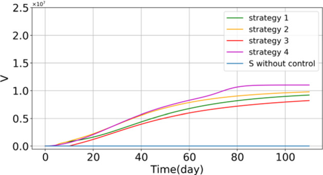
Fig. 4.

Compared solutions vaccination for Covid-19 by different strategies

Fig. 3.

Number of vaccinated people

In this sense, in Fig. 4a, Strategy 2 shows that its performance is better than the performance of Strategy 1 because this strategy reduces the number of susceptible people more than other strategies. This figure also demonstrates that if the exposed people are considered in the objective function, the optimal controller can perform better regarding the reduction in both susceptible and exposed populations. It should be noted that the more exposed the population decrease, the less susceptible individuals can be infected. Due to this fact, one can infer that both susceptible and exposed populations should be considered in objective functions.

Also, from a practical viewpoint, let us denote that the reinforcement learning optimal control can introduce a better policy for vaccination distribution regarding Pontryagin’s minimum principle. For example, in [59, 65, 66], the proposed optimal controls suggest the time evolution vaccination whose initial proportion is high and significant. This high initial value of vaccine usage makes Pontryagin’s minimum principle approach impractical and too harsh in the real world, but as presented in this article, reinforcement learning optimal control can propose a policy with smooth starting that provides functionality and practicality for public vaccination.

Graphical results depict the importance of vaccine allocation. In these graphical interpretation shows that if the vaccination is taken into account, the severity of infection can be reduced gradually. In the presented model, vaccination plays a vital role in the reduction in susceptible individuals. Consequently, one can see that when suspectable individuals who can transmit the virus and be infected start to fall, the number of infected people can decline in number. Decreasing the number of symptomatically infected people will reduce the exposure of uninfected people to infected people. Therefore, it can reduce the probability of being infected through the disease transmission too. As a result, the number of infected people is decreased significantly, which can end up with the elimination of the disease in society. It should be noted that due to the slow dynamic behavior of the epidemic model, it seems that the vaccine does not affect the population of infected people, but over time, the significance of vaccination effectiveness can be observable. Hence, this simulation highly suggests that governments and authorities should not be obsessed with the number of infected people during the early stage of vaccination because vaccines take time to induce immunity.

Conclusion

In this research, the significant challenge regarding vaccination strategies for COVID-19 has been investigated. Based on data from confirmed cases of 2019-nCoV in mainland China, a new deterministic SEIR model with additional vaccination components was developed. Following that, based on the reinforcement learning method, an optimal control was developed to discover the best policies. By implementing the dynamic model of the epidemiological system, numerical results for four different control strategies obtained by the proposed technique were demonstrated. The feasibility of the recommended method for designing optimal vaccine plans was clearly shown by these findings. As a future study, it would be useful to look at any of the behavioral or emotional side effects of quarantine, such as depression, which may impact depression or even suicide rate in society. Such investigations lead us to find an optimal trade-off for quarantine decisions.

References

- 1.Yuki K, Fujiogi M, Koutsogiannaki S. COVID-19 pathophysiology: a review. Clin. Immunol. 2020;2020:108427. doi: 10.1016/j.clim.2020.108427. [DOI] [PMC free article] [PubMed] [Google Scholar]
- 2.Xu P, Zhou Q, Xu J. Mechanism of thrombocytopenia in COVID-19 patients. Ann. Hematol. 2020;99:1205–1208. doi: 10.1007/s00277-020-04019-0. [DOI] [PMC free article] [PubMed] [Google Scholar]
- 3.Ciotti M, Angeletti S, Minieri M, Giovannetti M, Benvenuto D, Pascarella S, et al. COVID-19 outbreak: an overview. Chemotherapy. 2019;64:215–223. doi: 10.1159/000507423. [DOI] [PMC free article] [PubMed] [Google Scholar]
- 4.Velavan TP, Meyer CG. The COVID-19 epidemic. Trop. Med. Int. Health. 2020;25:278. doi: 10.1111/tmi.13383. [DOI] [PMC free article] [PubMed] [Google Scholar]
- 5.Gattinoni L, Coppola S, Cressoni M, Busana M, Rossi S, Chiumello D. COVID-19 does not lead to a “typical” acute respiratory distress syndrome. Am. J. Respir. Crit. Care Med. 2020;201:1299–1300. doi: 10.1164/rccm.202003-0817LE. [DOI] [PMC free article] [PubMed] [Google Scholar]
- 6.Xu Z, Shi L, Wang Y, Zhang J, Huang L, Zhang C, et al. Pathological findings of COVID-19 associated with acute respiratory distress syndrome. Lancet Respir. Med. 2020;8:420–422. doi: 10.1016/S2213-2600(20)30076-X. [DOI] [PMC free article] [PubMed] [Google Scholar]
- 7.Al-Tawfiq JA. Asymptomatic coronavirus infection: MERS-CoV and SARS-CoV-2 (COVID-19) Travel Med. Infect. Dis. 2020;35:101608. doi: 10.1016/j.tmaid.2020.101608. [DOI] [PMC free article] [PubMed] [Google Scholar]
- 8.Giannis D, Ziogas IA, Gianni P. Coagulation disorders in coronavirus infected patients: COVID-19, SARS-CoV-1, MERS-CoV and lessons from the past. J. Clin. Virol. 2020;127:104362. doi: 10.1016/j.jcv.2020.104362. [DOI] [PMC free article] [PubMed] [Google Scholar]
- 9.Gul N, Bilal R, Algehyne EA, Alshehri MG, Khan MA, Chu Y-M, et al. The dynamics of fractional order Hepatitis B virus model with asymptomatic carriers. Alex. Eng. J. 2021;60:3945–3955. doi: 10.1016/j.aej.2021.02.057. [DOI] [Google Scholar]
- 10.Ali A, Alshammari FS, Islam S, Khan MA, Ullah S. Modeling and analysis of the dynamics of novel coronavirus (COVID-19) with Caputo fractional derivative. Results Phys. 2021;20:103669. doi: 10.1016/j.rinp.2020.103669. [DOI] [PMC free article] [PubMed] [Google Scholar]
- 11.Alrabaiah H, Safi MA, DarAssi MH, Al-Hdaibat B, Ullah S, Khan MA, et al. Optimal control analysis of hepatitis B virus with treatment and vaccination. Results Phys. 2020;19:103599. doi: 10.1016/j.rinp.2020.103599. [DOI] [Google Scholar]
- 12.Chu Y-M, Ali A, Khan MA, Islam S, Ullah S. Dynamics of fractional order COVID-19 model with a case study of Saudi Arabia. Results Phys. 2021;21:103787. doi: 10.1016/j.rinp.2020.103787. [DOI] [PMC free article] [PubMed] [Google Scholar]
- 13.Khan MA, Atangana A. Modeling the dynamics of novel coronavirus (2019-nCov) with fractional derivative. Alex. Eng. J. 2020;59:2379–2389. doi: 10.1016/j.aej.2020.02.033. [DOI] [Google Scholar]
- 14.Alzahrani EO, Ahmad W, Khan MA, Malebary SJ. Optimal control strategies of Zika virus model with mutant. Commun. Nonlinear Sci. Numer. Simul. 2021;93:105532. doi: 10.1016/j.cnsns.2020.105532. [DOI] [Google Scholar]
- 15.Jahanshahi H. Smooth control of HIV/AIDS infection using a robust adaptive scheme with decoupled sliding mode supervision. Eur. Phys. J. Spec. Top. 2018;227:707–718. doi: 10.1140/epjst/e2018-800016-7. [DOI] [Google Scholar]
- 16.Jahanshahi H, Shanazari K, Mesrizadeh M, Soradi-Zeid S, Gómez-Aguilar JF. Numerical analysis of Galerkin meshless method for parabolic equations of tumor angiogenesis problem. Eur. Phys. J. Plus. 2020;135:1–23. doi: 10.1140/epjp/s13360-020-00716-x. [DOI] [Google Scholar]
- 17.Zhao TH, Castillo O, Jahanshah H. A fuzzy-based strategy to suppress the novel coronavirus (2019-NCOV) massive outbreak. Appl Comput Math. 2021;20:160–176. [Google Scholar]
- 18.Jahanshahi H, Munoz-Pacheco JM, Bekiros S, Alotaibi ND. A fractional-order SIRD model with time-dependent memory indexes for encompassing the multi-fractional characteristics of the COVID-19. Chaos Solitons Fract. 2021;143:110632. doi: 10.1016/j.chaos.2020.110632. [DOI] [PMC free article] [PubMed] [Google Scholar]
- 19.Wang H, Jahanshahi H, Wang M-K, Bekiros S, Liu J, Aly AA. A caputo-fabrizio fractional-order model of HIV/AIDS with a treatment compartment: sensitivity analysis and optimal control strategies. Entropy. 2021;23:610. doi: 10.3390/e23050610. [DOI] [PMC free article] [PubMed] [Google Scholar]
- 20.Pandey P, Chu Y-M, Gómez-Aguilar JF, Jahanshahi H, Aly AA. A novel fractional mathematical model of COVID-19 epidemic considering quarantine and latent time. Results Phys. 2021;221:104286. doi: 10.1016/j.rinp.2021.104286. [DOI] [PMC free article] [PubMed] [Google Scholar]
- 21.Grassly NC, Fraser C. Mathematical models of infectious disease transmission. Nat. Rev. Microbiol. 2008;6:477–487. doi: 10.1038/nrmicro1845. [DOI] [PMC free article] [PubMed] [Google Scholar]
- 22.Chen S-B, Rajaee F, Yousefpour A, Alcaraz R, Chu Y-M, Gómez-Aguilar JF, et al. Antiretroviral therapy of HIV infection using a novel optimal type-2 fuzzy control strategy. Alex. Eng. J. 2021;60:1545–1555. doi: 10.1016/j.aej.2020.11.009. [DOI] [Google Scholar]
- 23.Khan MA, Alfiniyah C, Alzahrani E. Analysis of dengue model with fractal-fractional Caputo-Fabrizio operator. Adv. Differ. Equ. 2020;2020:1–23. [Google Scholar]
- 24.Eubank S, Guclu H, Kumar VSA, Marathe MV, Srinivasan A, Toroczkai Z, et al. Modelling disease outbreaks in realistic urban social networks. Nature. 2004;429:180–184. doi: 10.1038/nature02541. [DOI] [PubMed] [Google Scholar]
- 25.Ullah S, Khan MA. Modeling the impact of non-pharmaceutical interventions on the dynamics of novel coronavirus with optimal control analysis with a case study. Chaos Solitons Fract. 2020;139:110075. doi: 10.1016/j.chaos.2020.110075. [DOI] [PMC free article] [PubMed] [Google Scholar]
- 26.Awais M, Alshammari FS, Ullah S, Khan MA, Islam S. Modeling and simulation of the novel coronavirus in Caputo derivative. Results Phys. 2020;19:103588. doi: 10.1016/j.rinp.2020.103588. [DOI] [PMC free article] [PubMed] [Google Scholar]
- 27.Yousefpour A, Jahanshahi H, Bekiros S. Optimal policies for control of the novel coronavirus disease (COVID-19) outbreak. Chaos Solitons Fract. 2020;136:109883. doi: 10.1016/j.chaos.2020.109883. [DOI] [PMC free article] [PubMed] [Google Scholar]
- 28.Ndaïrou F, Area I, Nieto JJ, Torres DFM. Mathematical modeling of COVID-19 transmission dynamics with a case study of Wuhan. Chaos Solitons Fract. 2020;135:109846. doi: 10.1016/j.chaos.2020.109846. [DOI] [PMC free article] [PubMed] [Google Scholar]
- 29.Tuan NH, Mohammadi Rezapourdidi H. A mathematical model for COVID-19 transmission by using the Caputo fractional derivative. Chaos Solitons Fract. 2020;140:110107. doi: 10.1016/j.chaos.2020.110107. [DOI] [PMC free article] [PubMed] [Google Scholar]
- 30.Alqarni MS, Alghamdi M, Muhammad T, Alshomrani AS, Khan MA. Mathematical modeling for novel coronavirus (COVID-19) and control. Numer: Methods Partial Differ. Equ; 2020. [DOI] [PMC free article] [PubMed] [Google Scholar]
- 31.Panovska-Griffiths J. Can Mathematical Modelling Solve the Current Covid-19 Crisis? Berlin: Springer; 2020. [DOI] [PMC free article] [PubMed] [Google Scholar]
- 32.Khan MA, Atangana A, Alzahrani E. The dynamics of COVID-19 with quarantined and isolation. Adv. Differ. Equ. 2020;2020:1–22. doi: 10.1186/s13662-020-02882-9. [DOI] [PMC free article] [PubMed] [Google Scholar]
- 33.Oud MAA, Ali A, Alrabaiah H, Ullah S, Khan MA, Islam S. A fractional order mathematical model for COVID-19 dynamics with quarantine, isolation, and environmental viral load. Adv. Differ. Equ. 2021;2021:1–19. doi: 10.1186/s13662-021-03265-4. [DOI] [PMC free article] [PubMed] [Google Scholar]
- 34.Khan MA, Ullah S, Kumar S. A robust study on 2019-nCOV outbreaks through non-singular derivative. Eur. Phys. J. Plus. 2021;136:1–20. doi: 10.1140/epjp/s13360-021-01159-8. [DOI] [PMC free article] [PubMed] [Google Scholar]
- 35.Dunford D, Dale B, Stylianou N, Lowther E, Ahmed M, De la Torre AI. Coronavirus: the world in lockdown in maps and charts. BBC News. 2020;9:462. [Google Scholar]
- 36.Tang B, Wang X, Li Q, Bragazzi NL, Tang S, Xiao Y, et al. Estimation of the transmission risk of the 2019-nCoV and its implication for public health interventions. J. Clin. Med. 2020;9:462. doi: 10.3390/jcm9020462. [DOI] [PMC free article] [PubMed] [Google Scholar]
- 37.Tang B, Bragazzi NL, Li Q, Tang S, Xiao Y, Wu J. An updated estimation of the risk of transmission of the novel coronavirus (2019-nCov) Infect. Dis. Model. 2020;5:248–255. doi: 10.1016/j.idm.2020.02.001. [DOI] [PMC free article] [PubMed] [Google Scholar]
- 38.Volz E, Mishra S, Chand M, Barrett JC, Johnson R, Geidelberg L, et al. Assessing transmissibility of SARS-CoV-2 lineage B. 1.1. 7 in England. Nature. 2021;593:266–269. doi: 10.1038/s41586-021-03470-x. [DOI] [PubMed] [Google Scholar]
- 39.Davies NG, Abbott S, Barnard RC, Jarvis CI, Kucharski AJ, Munday JD, et al. Estimated transmissibility and impact of SARS-CoV-2 lineage B. 1.1. 7 in England. Science. 2021;372:eabg3055. doi: 10.1126/science.abg3055. [DOI] [PMC free article] [PubMed] [Google Scholar]
- 40.Abu-Khalaf M, Lewis FL. Nearly optimal control laws for nonlinear systems with saturating actuators using a neural network HJB approach. Automatica. 2005;41:779–791. doi: 10.1016/j.automatica.2004.11.034. [DOI] [Google Scholar]
- 41.R. Beard, Improving the closed-loop performance of nonlinear systems, Ph.D. dissertation, Rensselaer Polytech. Inst., Troy, NY (1995)
- 42.Yaghmaie FA, Braun DJ. Reinforcement learning for a class of continuous-time input constrained optimal control problems. Automatica. 2019;99:221–227. doi: 10.1016/j.automatica.2018.10.038. [DOI] [Google Scholar]
- 43.Drazin PG, Drazin PD. Nonlinear systems. Cambridge: Cambridge University Press; 1992. [Google Scholar]
- 44.Ioannou PA, Sun J. Robust Adaptive Control. London: Courier Corporation; 2012. [Google Scholar]
- 45.Zhong X, He H. An event-triggered ADP control approach for continuous-time system with unknown internal states. IEEE Trans. Cybern. 2016;47:683–694. doi: 10.1109/TCYB.2016.2523878. [DOI] [PubMed] [Google Scholar]
- 46.Wei Q, Zhang H, A New Approach to Solve a Class of Continuous-Time Nonlinear Quadratic Zero-Sum Game Using ADP. IEEE. pp. 507–512.
- 47.V.R. Konda, J.N. Tsitsiklis, Actor-Critic Algorithms, Citeseer. pp. 1008–10014.
- 48.Hornik K, Stinchcombe M, White H. Universal approximation of an unknown mapping and its derivatives using multilayer feedforward networks. Neural Netw. 1990;3:551–560. doi: 10.1016/0893-6080(90)90005-6. [DOI] [Google Scholar]
- 49.Zhu Y, Zhao D, Li X. Using reinforcement learning techniques to solve continuous-time non-linear optimal tracking problem without system dynamics. IET Control Theory Appl. 2016;10:1339–1347. doi: 10.1049/iet-cta.2015.0769. [DOI] [Google Scholar]
- 50.Xiao G, Zhang H, Luo Y, Qu Q. General value iteration based reinforcement learning for solving optimal tracking control problem of continuous–time affine nonlinear systems. Neurocomputing. 2017;245:114–123. doi: 10.1016/j.neucom.2017.03.038. [DOI] [Google Scholar]
- 51.Kiumarsi B, Lewis FL. Actor–critic-based optimal tracking for partially unknown nonlinear discrete-time systems. IEEE Trans. Neural Netw. Learn. Syst. 2014;26:140–151. doi: 10.1109/TNNLS.2014.2358227. [DOI] [PubMed] [Google Scholar]
- 52.Yang X, Liu D, Luo B, Li C. Data-based robust adaptive control for a class of unknown nonlinear constrained-input systems via integral reinforcement learning. Inf. Sci. 2016;369:731–747. doi: 10.1016/j.ins.2016.07.051. [DOI] [Google Scholar]
- 53.A. Wuraola, N. Patel, SQNL: A new computationally efficient activation function. IEEE, pp. 1–7.
- 54.D.L. Elliott, A better activation function for articial neural networks. ISR technical report TR 93-8, Univeristy of Maryland (1993)
- 55.Vamvoudakis KG, Lewis FL. Online actor–critic algorithm to solve the continuous-time infinite horizon optimal control problem. Automatica. 2010;46:878–888. doi: 10.1016/j.automatica.2010.02.018. [DOI] [Google Scholar]
- 56.Bhasin S, Kamalapurkar R, Johnson M, Vamvoudakis KG, Lewis FL, Dixon WE. A novel actor–critic–identifier architecture for approximate optimal control of uncertain nonlinear systems. Automatica. 2013;49:82–92. doi: 10.1016/j.automatica.2012.09.019. [DOI] [Google Scholar]
- 57.Shi J, Yue D, Xie X. Adaptive optimal tracking control for nonlinear continuous-time systems with time delay using value iteration algorithm. Neurocomputing. 2020;396:172–178. doi: 10.1016/j.neucom.2018.07.098. [DOI] [Google Scholar]
- 58.Lewis FW, Jagannathan S, Yesildirak A. Neural Network Control of Robot Manipulators and Non-linear Systems. London: CRC Press; 2020. [Google Scholar]
- 59.Yang Y, Tang S, Ren X, Zhao H, Guo C. Global stability and optimal control for a tuberculosis model with vaccination and treatment. Discrete Contin. Dyn. Syst. B. 2016;21:1009. doi: 10.3934/dcdsb.2016.21.1009. [DOI] [Google Scholar]
- 60.Rostamy D, Mottaghi E. Stability analysis of a fractional-order epidemics model with multiple equilibriums. Adv. Differ. Equ. 2016;2016:1–11. doi: 10.1186/s13662-016-0905-4. [DOI] [Google Scholar]
- 61.Dormand JR, Prince PJ. A reconsideration of some embedded Runge–Kutta formulae. J. Comput. Appl. Math. 1986;15:203–211. doi: 10.1016/0377-0427(86)90027-0. [DOI] [Google Scholar]
- 62.Polack FP, Thomas SJ, Kitchin N, Absalon J, Gurtman A, Lockhart S, et al. Safety and efficacy of the BNT162b2 mRNA Covid-19 vaccine. N. Engl. J. Med. 2020;383:2603–2615. doi: 10.1056/NEJMoa2034577. [DOI] [PMC free article] [PubMed] [Google Scholar]
- 63.Xu W, Su S, Jiang S. Ring vaccination of COVID-19 vaccines in medium-and high-risk areas of countries with low incidence of SARS-CoV-2 infection. Clin. Transl. Med. 2021;11:2. doi: 10.1002/ctm2.331. [DOI] [PMC free article] [PubMed] [Google Scholar]
- 64.Kucharski AJ, Eggo RM, Watson CH, Camacho A, Funk S, Edmunds WJ. Effectiveness of ring vaccination as control strategy for Ebola virus disease. Emerg. Infect. Dis. 2016;22:105. doi: 10.3201/eid2201.151410. [DOI] [PMC free article] [PubMed] [Google Scholar]
- 65.Sari RA, Habibah U, Widodo A. Optimal control on model of SARS disease spread with vaccination and treatment. J. Exp. Life Sci. 2017;7:61–68. doi: 10.21776/ub.jels.2017.007.02.01. [DOI] [Google Scholar]
- 66.Ahmad MD, Usman M, Khan A, Imran M. Optimal control analysis of Ebola disease with control strategies of quarantine and vaccination. Infect. Dis. Poverty. 2016;5:1–12. doi: 10.1186/s40249-016-0161-6. [DOI] [PMC free article] [PubMed] [Google Scholar]