A taxonomy of transcriptomic cell types across the isocortex and hippocampal formation

SUMMARY

The isocortex and hippocampal formation (HPF) in the mammalian brain play critical roles in perception, cognition, emotion and learning. We profiled ~1.3 million cells covering the entire adult mouse isocortex and HPF and derived a transcriptomic cell type taxonomy revealing a comprehensive repertoire of glutamatergic and GABAergic neuron types. Contrary to the traditional view of HPF as having a simpler cellular organization, we discover a complete set of glutamatergic types in HPF homologous to all major subclasses found in the six-layered isocortex, suggesting that HPF and isocortex share a common circuit organization. We also identify large-scale continuous and graded variation of cell types along isocortical depth, across isocortical sheet and in multiple dimensions in hippocampus and subiculum. Overall, our study establishes a molecular architecture of mammalian isocortex and hippocampal formation and begins to shed light on its underlying relationship with the development, evolution, connectivity and function of these brain structures.

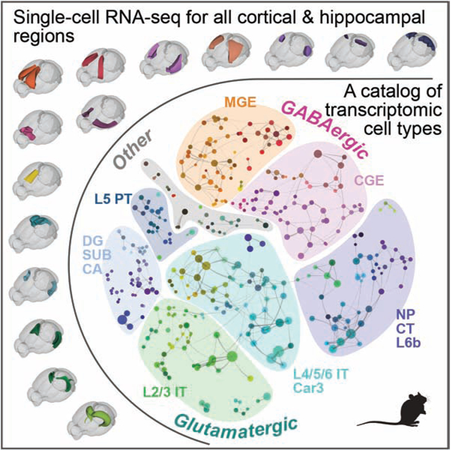
Graphical Abstract

ETOC:

Single-cell transcriptomics of entire mouse isocortex and hippocampal formation shows shared cellular and circuit organization and large-scale continuous gradients of neuron type variation that illuminates the underlying relationship between these two critical brain structures.

INTRODUCTION

The cerebral cortex occupies a large portion of the mammalian brain and executes multiple functions, from sensory perception and generation of voluntary behavior to emotion, cognition, learning and memory. The cortex is partitioned into multiple areas with specific input and output connections with many subcortical and other cortical regions (Rakic, 2009; Van Essen and Glasser, 2018). This area specialization is likely a major contributing factor to the diversity of functions supported by cortex (Cadwell et al., 2019).

Developmentally, cortex originates from pallium, a main part of the telencephalon, which can be divided into several parts (Pessoa et al., 2019). Medial pallium gives rise to hippocampal formation (also called archicortex), ventral pallium gives rise to olfactory cortex (also called paleocortex), and in mammals, dorsal pallium gives rise to isocortex (also called neocortex). Archicortex and paleocortex are considered evolutionarily older structures, whereas iso/neocortex emerged later and substantially expanded in vertebrate evolution, culminating in its current form in mammals (Rakic, 2009) with a general belief that archicortex and paleocortex neurons are arranged in 3 to 5 layers and iso/neocortex in 6 layers.

Functional areas of the iso/neocortex (~180 in humans and ~30 in mice) (Van Essen and Glasser, 2018) tile the cortical sheet and include primary and higher-order sensory areas across all sensory modalities, primary and secondary motor areas, as well as multiple associational areas in the frontal, medial, and lateral parts of the isocortex that perform a variety of integrative functions. Extensive connectivity tracing and in vivo neural imaging studies have shown that these neocortical areas together form a hierarchical neural network with functionally distinct modules and feedforward and feedback pathways both within and between modules (Coogan and Burkhalter, 1993; Felleman and Van Essen, 1991; Harris et al., 2019; Markov et al., 2014; Siegle et al., 2021).

Hippocampal formation (HPF) is also a complex multi-areal structure, which includes the hippocampal region, the subicular complex, and the medial and lateral entorhinal cortex. Neurons in these regions are interconnected to form a network that underlies many functions of HPF – learning, memory, spatial navigation, and regulation of emotions (Bienkowski et al., 2018; van Strien et al., 2009). In particular, there is a prominent functional transition along the dorsal-ventral axis of HPF, with the dorsal network mainly mediating spatial navigation and the ventral network mainly mediating emotional behaviors (Cembrowski and Spruston, 2019).

Many molecular, anatomical, and physiological studies have revealed a broad spectrum of neuronal cell types in different cortical and hippocampal regions, whose variety of cellular properties are likely related to specific functions in the circuits they are embedded in (Zeng and Sanes, 2017). But a systematic study is needed for a complete picture of the number and distribution of cell types in these regions and for understanding how different cortical and hippocampal regions interact with the rest of the brain and carry out their individual functions.

Both isocortex and HPF have two major classes of neurons, glutamatergic excitatory and GABAergic inhibitory, each containing multiple types. Glutamatergic neuronal types are organized by layers and their long-range projection patterns (Harris and Shepherd, 2015); their tremendous diversity in interareal axon-projection patterns forms the structural basis of the hierarchical network (D’Souza et al., 2016; Harris et al., 2019). Isocortical and hippocampal GABAergic interneuron types are similarly organized by their embryonic origins, firing characteristics and local connectivity patterns (Fishell and Rudy, 2011; Pelkey et al., 2017; Tremblay et al., 2016).

Single-cell RNA-sequencing (scRNA-seq) studies have systematically characterized and classified cell types in individual regions of isocortex and hippocampus (Harris et al., 2018; Hodge et al., 2019; Tasic et al., 2016; Tasic et al., 2018; Yao et al., 2020; Zeisel et al., 2015). Previously, we analyzed single-cell transcriptomes to define 133 cell types in two isocortical areas, primary visual cortex (VISp) and anterolateral motor cortex (ALM), in mice (Tasic et al., 2018) and found that they have shared GABAergic interneuron types but distinct glutamatergic neuron types. More recently, using the Patch-seq approach, we simultaneously profiled the transcriptomic, electrophysiological, and morphological properties of a large set of GABAergic interneurons from mouse visual cortex and found excellent correspondence among the three modalities (Gouwens et al., 2020). Similar findings were made in another Patch-seq study focused on mouse primary motor cortex (MOp) (Scala et al., 2020). These studies demonstrate the validity and power of using the highly scalable scRNA-seq approach to generate a comprehensive census of cell types as a foundation for further structural and functional studies of brain circuits.

Here we cover all of the adult mouse isocortex and HPF, analyzing >1.3 million cells with two different scRNA-seq platforms (10x and SMART-Seq). We developed a consensus clustering approach to combine the two datasets and derived a cell type taxonomy comprising 388 transcriptomic types of which 364 are neuronal. The coverage enabled defining neuronal cell type composition across the entire spatial landscape without significant gaps, including the discovery of many, to the best of our knowledge, newly identified cell types in associational cortical areas and HPF. Comparing between isocortex and HPF, we find that all GABAergic neuron types in isocortex are shared with HPF, whereas HPF also contains additional GABAergic types unique to itself. On the other hand, glutamatergic neuron types from different HPF regions are highly distinct from but also, surprisingly, homologous to those in isocortex. This homologous relationship is supported by both shared molecular signatures, including canonical transcription factors, and similar layer-specific distributions. Many isocortical glutamatergic types are shared across multiple areas and exhibit gradient-like gene expression variations along the cortical sheet. Similarly, hippocampal and subicular glutamatergic types are organized along multiple spatial dimensions. Our study reveals the molecular organizational structure of the entire isocortex and HPF, suggesting an evolutionarily conserved cellular and circuit organization between these two major brain structures.

RESULTS

Generation of the transcriptomic cell type taxonomy

To conduct large-scale single-cell transcriptomic characterization of cell types, we used two complementary approaches: SMART-Seq v4 (SSv4) (Tasic et al., 2018), and 10x Genomics Chromium platform based on version 2 chemistry (10xv2) (STAR Methods, Methods S1).

Brain regions for profiling and boundaries for dissections were defined by Allen Mouse Brain Common Coordinate Framework version 3 (CCFv3) (Wang et al., 2020) and sampled at mid-ontology level covering all regions of isocortex (CTX) and HPF (Fig. 1A, Table S1, Methods S1), listed here for reference. Covered areas in CTX: frontal pole (FRP), primary motor (MOp), secondary motor (MOs), primary somatosensory (SSp), supplemental somatosensory (SSs), gustatory (GU), visceral (VISC), auditory (AUD), primary visual (VISp), anterolateral visual (VISal), anteromedial visual (VISam), lateral visual (VISl), posterolateral visual (VISpl), posteromedial (VISpm), laterointermediate (VISli), postrhinal (VISpor), anterior cingulate (ACA), prelimbic (PL), infralimbic (ILA), orbital (ORB), agranular insular (AI), retrosplenial (RSP), posterior parietal association (PTLp), temporal association (TEa), perirhinal (PERI), and ectorhinal (ECT) areas. Covered regions in HPF are divided into two main parts: the hippocampal region (HIP), including fields CA1, CA2, CA3, and dentate gyrus (DG), and the retrohippocampal region (RHP), including lateral entorhinal area (ENTl), medial entorhinal area (ENTm), parasubiculum (PAR), postsubiculum (POST), presubiculum (PRE), subiculum (SUB), and prosubiculum (ProS). The few remaining small regions in HPF, i.e., fasciola cinereal (FC), induseum griseum (IG), hippocampo-amygdalar transition area (HATA), and area prostriata (APr), were included in the dissection of their neighboring regions.

Figure 1. Transcriptomic cell type taxonomy of the isocortex and hippocampal formation.

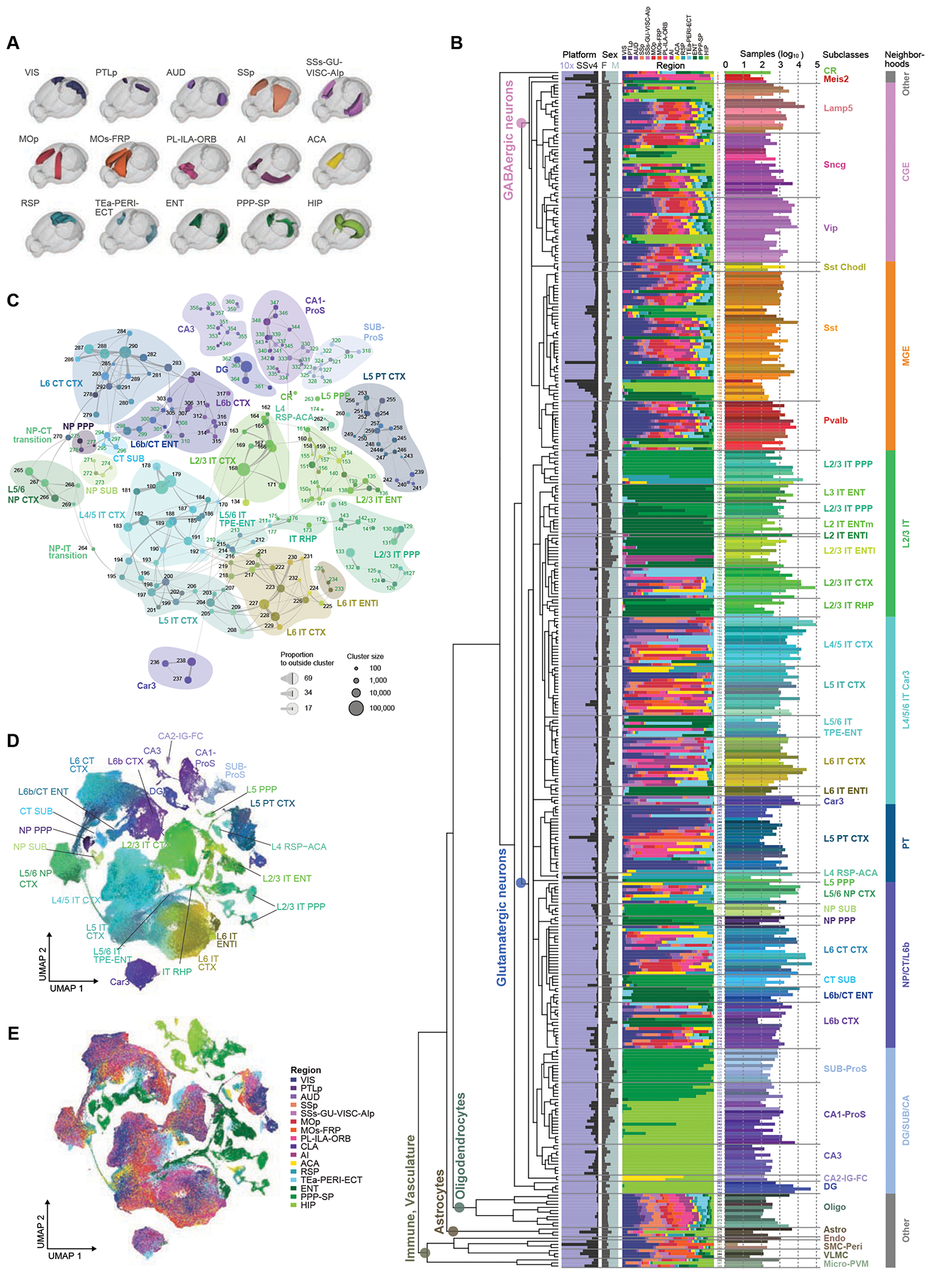
(A) Overview of sampled brain regions rendered in Allen CCFv3. The PPP-SP joint region includes PAR-POST-PRE-SUB-ProS.

(B) The transcriptomic taxonomy tree of 388 clusters organized in a dendrogram (10xv2: n = 1,169,213; SSv4: n = 73,346). Bar plots represent fractions of cells profiled according to platform, sex, and region, and the total number of cells per cluster on a log₁₀ scale.

(C) Constellation plot of the global relatedness between glutamatergic types. Each cluster is represented by a dot, positioned at the cluster centroid in UMAP coordinates shown in D. Clusters are grouped by subclass. Clusters with more than 80% of cells derived from HPF are labeled green.

(D-E) UMAP representation of glutamatergic types colored by cluster (D) or region (E).

See also Tables S1–S4, Methods S1, Data S1, Figure S2.

We used transgenic driver lines for cell isolation by fluorescence-activated cell sorting (FACS) to enrich for neurons (STAR Methods, Methods S1, Table S2) to obtain 1,228,636 single-cell 10xv2 transcriptomes and 76,381 single-cell SSv4 transcriptomes after the quality control (QC) process. We first clustered 10xv2 and SSv4 cells separately, resulting in 332 10xv2 clusters and 324 SSv4 clusters. Integrative clustering of the 10xv2 and SSv4 datasets resulted in 388 consensus clusters (Fig. 1B, Table S3). Despite the large difference in gene detection for the two platforms (8,894 ± 1,551 genes per cell for SSv4 and 4,125 ± 1,176 for 10xv2, average ± SD), there was good correlation for the numbers of genes detected at each cluster level between the two methods (Methods S1, Detection rates).

Post-clustering, we constructed a taxonomy tree (Fig. 1B) by hierarchical clustering of transcriptomic clusters based on the average gene expression per cluster of 5,981 differentially expressed (DE) genes (Table S4). We explored the relationships among the 388 clusters by visualizing cells belonging to them with Uniform Manifold Approximation and Projection (UMAP) and constellation plots (Fig. 1C–E, Data S1, Taxonomy). These different approaches for exploring a cell type landscape, which is a combination of discrete and continuous gene expression variation, provide a holistic description of the taxonomy. Taxonomical trees are simple but artificially discrete: they do not preserve all the multidimensional relationships among types, but they highlight the dominant hierarchical relationships which are less clear in UMAP representations. UMAPs and constellation plots enable visualization of continuity in addition to discreteness. With this base, we label sets of cells within the taxonomy from coarse to fine categories as: class, neighborhood, subclass, supertype, and type (Fig. 1B).

To annotate this taxonomy containing many new transcriptomic types, we collated sets of DE genes selective for each cluster and each branch of the taxonomy to represent different levels of granularity, and examined their anatomical expression patterns using the Allen Brain Atlas (ABA) RNA in situ hybridization (ISH) data (Lein et al., 2007). Based on this anatomical (both regional and laminar) annotation and prior knowledge, we assigned the 388 clusters into 4 classes, 8 neighborhoods, 42 subclasses, and 101 supertypes. The GABAergic neuronal class contains 6 subclasses and 119 clusters; the glutamatergic neuronal class contains 28 subclasses and 241 clusters; the astrocyte/oligodendrocyte non-neuronal class contains 2 subclasses and 14 clusters; and the immune/vascular non-neuronal class contains 4 subclasses and 10 clusters (Fig. 1B, Table S3). We grouped the subclasses into 8 neighborhoods, 2 GABAergic (CGE and MGE), 5 glutamatergic (L2/3 IT, L4/5/6 IT Car3, PT, NP/CT/L6b, and DG/SUB/CA), and one ‘Other’ neighborhood.

Detailed analyses of the neuronal neighborhoods are presented in sections below. The ‘Other’ neighborhood, briefly mentioned here, includes all non-neuronal subclasses, as well as two neuronal subclasses, Cajal-Retzius (CR) (glutamatergic, mostly in layer 1) and Meis2 (GABAergic, mostly in white matter) (Fig. 1B, Table S3). Meis2 neurons were identified as related to olfactory bulb interneurons (Frazer et al., 2017). For the astro/oligo class, we identified 3 astrocyte clusters and 11 oligodendrocyte clusters. For the immune/vascular class, there were 1 endothelial cell cluster, 3 smooth muscle cell (SMC) and pericyte clusters, 3 vascular/leptomeningeal cell (VLMC) clusters and 3 microglia/perivascular macrophage (PVM) clusters. Since the cell isolation in this study aimed toward enrichment for neurons, we had limited sampling of non-neuronal cells (15,241 10xv2 cells and 1,828 SSv4 cells after QC) and this study is focused on neuronal cell types.

Comparing this taxonomy with six previous studies (Cembrowski et al., 2018; Harris et al., 2018; Saunders et al., 2018; Tasic et al., 2018; Yao et al., 2020; Zeisel et al., 2018), we found generally good but variable correspondences (Data S1, Taxonomy comparison). While these studies focused on one or two individual regions, our current taxonomy provides an overview of cell type variation across regions.

GABAergic cell type taxonomy

The GABAergic inhibitory neuronal class is divided into two neighborhoods that correlate with distinct developmental origins: caudal ganglionic eminence (CGE) (Fig. 2A–E) and medial ganglionic eminence (MGE) (Fig. 2F–J). Note that some of the CGE cell types (e.g., some neurogliaform cells) may, in fact, be developmentally derived from the nearby preoptic region (PO) (Niquille et al., 2018). Each neighborhood is further divided into 3 subclasses: Lamp5, Sncg and Vip in CGE, and Sst Chodl, Sst and Pvalb in MGE.

Figure 2. GABAergic cell types of isocortex and hippocampal formation.

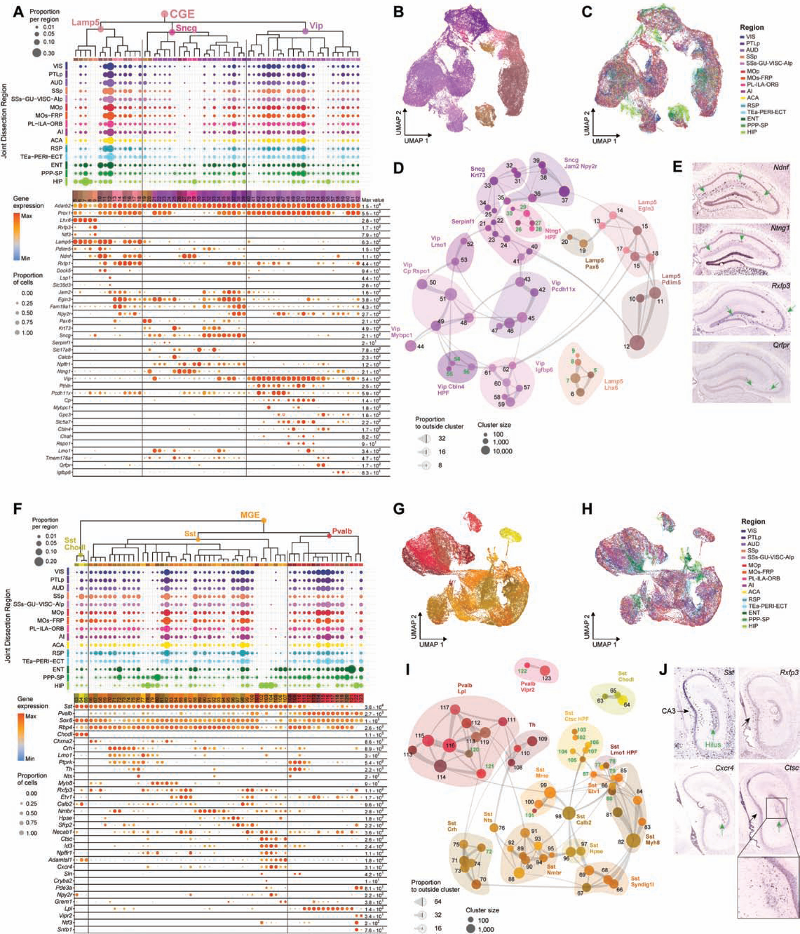
(A) Dendrogram of CGE clusters followed by dot plots showing proportion of cells within each cluster derived from each region of dissection and marker gene expression in each cluster from the 10xv2 dataset. Dot size and color indicate proportion of expressing cells and average expression level in each cluster, respectively.

(B-C) UMAP representation of CGE clusters, colored by cluster (B) or region (C).

(D) Constellation plot of CGE clusters using UMAP coordinates shown in B. Clusters are grouped by supertype. Clusters with more than 80% of cells derived from HPF are labeled green.

(E) RNA ISH from Allen Mouse Brain Atlas (ABA) for select markers expressed in the HPF-specific CGE supertypes.

(F-J) Same as A-E but for MGE clusters.

See also Figure S1, Data S1.

In the CGE neighborhood, the Lamp5 (mostly neurogliaform cells), Sncg and Vip subclasses are divided into 4, 5 (one containing Vip cells), and 6 supertypes, respectively (Fig. 2D, Table S3). In the MGE neighborhood, the Sst Chodl subclass remains as one group (representing long-range projecting Sst cells); the Sst and Pvalb subclasses are divided into 11 and 3 supertypes, respectively (Fig. 2I, Table S3). The current CTX-HPF GABAergic taxonomy is largely consistent with previous transcriptomic taxonomies derived from cortical areas VISp-ALM (Tasic et al., 2018) and MOp (Yao et al., 2020) at the supertype level but exhibits notable ambiguity at the type/cluster level (Fig. S1). It is also consistent with the large body of literature on cortical GABAergic interneurons (Lim et al., 2018; Pelkey et al., 2017; Tremblay et al., 2016), and our Patch-seq study (Gouwens et al., 2020) with MET types defined in that study corresponding well with the supertypes defined here (Fig. S1).

As shown in dot plots (Fig. 2A, F) and UMAPs (Fig. 2C, H), most clusters are shared by all isocortical areas, consistent with our previous observations (Tasic et al., 2018), and also by RHP regions. Even the relative proportions of cells in these clusters, based the large number of 10xv2 cells, appear consistent across the different regions (Fig. 2A, F). At the same time, we also observe a set of clusters that are specific to or highly enriched in HPF. These include the Lamp5 Lhx6, Ntng1 HPF, Vip Cbln4 HPF, Sst Lmo1 HPF and Sst Ctsc HPF supertypes, and select clusters within shared supertypes (Fig. 2A, D, F, I). Conversely, some clusters are largely absent from HIP (e.g. Lamp5 Pax6, Sst Syndig1l and Sst Hpse supertypes), while others have CTX- or HPF-selective counterparts (e.g. Sst Myh8 and Sst Etv1 clusters in CTX versus those in HPF). The greatest distinction in GABAergic interneuron type composition is between CTX and HIP itself; the RHP regions often contain both CTX and HIP clusters, with a few exceptions.

Our CTX-HPF GABAergic taxonomy corresponds well with a previous scRNA-seq study of CA1 interneurons (Harris et al., 2018), particularly for some HPF-specific clusters identified here (Data S1, Taxonomy comparison). For CGE, the Ntng1 HPF supertype does not express canonical pan-CGE marker Prox1 (Miyoshi et al., 2015; Rubin and Kessaris, 2013) nor its subclass markers Vip, Sncg or Lamp5 (Fig. 2A). Ntng1+ cells in HIP are seen at the stratum radiatum/stratum lacunosum-moleculare border (Fig. 2E) and may be the trilaminar cells or radiatum-retrohippocampal neurons projecting to RSP. The Lamp5 Lhx6 supertype is much more abundant in HIP than in cortex and is likely derived from MGE instead of CGE (Pelkey et al., 2017); its clusters #5, 8 and 9 are HPF-specific and are marked by Rxfp3 which is found in CA3 (Fig. 2E). Clusters #54–55 in supertype Vip Cbln4 HPF are marked by Qrfpr, also expressed in CA3 (Fig. 2E).

The Sst subclass has multiple HPF-enriched clusters, most of which are marked by Npffr1. Since isocortical Sst Myh8 and Etv1 cells are L5 Martinotti cells (Gouwens et al., 2020) (Fig. S1B), the HPF Myh8 and Etv1 cells are likely the Martinotti-like oriens lacunosum-moleculare (OLM) cells (Leao et al., 2012). Sst Ctsc HPF is a highly distinct HPF-specific supertype; clusters #102–103 are marked by Rxfp3 which is expressed in CA3, while clusters #104–105 are marked by Cxcr4 expressed in the polymorphic layer of DG (DG-po, also known as the hilus) (Fig. 2J). The Cxcr4+ cells may correspond to the hilar performant path-associated (HIPP) or DG somatostatin-expressing-interneurons (DG-SOMIs) described previously (Yuan et al., 2017). We also identified a HIP-specific Pvalb chandelier cell cluster #122 with unique markers Ntf3 and Sntb1.

Glutamatergic cell type taxonomy

The glutamatergic neuronal class is much more complex than the GABAergic class (Table S3). Excluding the CR type, we defined 5 neighborhoods, 28 subclasses, 56 supertypes and 241 types/clusters in the glutamatergic class and visualized them in a taxonomy tree (Fig. 1B), a UMAP and a constellation plot (Fig. 1C–D), together with marker gene expression (Data S1, Glutamatergic subclasses) and regional distribution (Fig. 1E, S2) for each subclass and type.

The L2/3 IT and L4/5/6 IT Car3 neighborhoods are composed of intratelencephalic (IT) and related neuronal types from all layers of all CTX regions as well as RHP regions. They constitute the largest proportion of cell types, with 14 subclasses that correspond well to specific layers (L2–6) and/or regions. The distinct subclass of Car3, which includes neurons from L6 of many lateral cortical areas, is included here as our previous study showed that these Car3+ L6 neurons, like cortical IT neurons, have extensive intracortical axon projections (Peng et al., 2020). The PT neighborhood contains the subclass of CTX L5 pyramidal tract (PT) neurons (also known as extratelencephalic or subcerebral projection neurons, SCPNs) and two related, region-specific subclasses, L4 RSP-ACA and L5 PPP. The NP/CT/L6b neighborhood includes both CTX and HPF cells that are divided into 7 subclasses: CTX L5/6 near-projecting (NP), L6 corticothalamic (CT), L6b neuron subclasses, and related subclasses from HPF. Lastly, the DG/SUB/CA neighborhood comprises cells that are specifically located in CA1, CA2, CA3, ProS, SUB and DG which are divided into 5 region-specific subclasses. The SUB-ProS and CA1-ProS subclasses both contain clusters from ProS, suggesting ProS contains cell types similar to either SUB or CA1, as in our previous study (Ding et al., 2020).

We systematically identified a large number of neuronal types and subclasses from different HPF regions that are highly distinct from those in CTX and from each other. At the same time, the presence of these cell types in close proximity with isocortical neuron types (particularly in the L2/3 IT, L4/5/6 IT and NP/CT/L6b neighborhoods) in taxonomy tree and UMAP suggests homologous relationships between HPF and CTX cell types (Fig. 1B–E). We further explored this by searching for gene expression covariation between HPF and CTX despite of regional difference and correlating gene expression for each HPF cell to the average expression of each CTX cluster (STAR Methods). The CTX cluster with the highest correlation to each HPF cluster was selected as the match, and the matches were aggregated by CTX subclasses (Fig. 3A). This approach revealed that most HPF cell types match a specific CTX subclass. We then calculated the number of DE genes between the highest correlated HPF-CTX cluster pair, which could indicate the overall degree of relatedness or similarity of the pair (the fewer DE genes, the more related).

Figure 3. Comparison of glutamatergic cell types in isocortex and hippocampal formation.

(A) Correspondence of HPF clusters to CTX subclasses, represented as a proportion of total matches. Lower panel shows the number of differentially expressed genes between each HPF cluster and its best-matched CTX cluster.

(B) Overview of glutamatergic cell types across all regions in CTX and HPF. Cell types are shown by supertypes and clusters within each supertype. CTX and HPF are separated by a solid line. Cell types in each CTX and RHP region (but not HIP) are displayed according to their layer specificity from top down. Cell types from RHP regions are aligned with those from CTX based on their similarity in layer specificity. IT types are shaded with pinkish ovals, PT, NP, CT and L6b types with yellowish ovals, and HIP types with blueish ovals. Each oval spans the major region(s) cells in each supertype come from. Within CTX, most supertypes span all areas. Some clusters within a given supertype exhibit preference for one or a few areas, and these clusters are shown as smaller ovals contained within the larger supertype oval. Cell types with similar projection patterns (intratelecephalic, extratelencephalic/subcerebral, or corticothalamic) are grouped by large brackets.

See also Figures S2–S3.

CTX NP, CT and L6b subclasses have the greatest similarity with their counterparts in ENT, PPP and SUB, as do CTX L2/3, L4/5 and L6 IT subclasses (Fig. 3A). Interestingly, L3 IT ENT, L2 IT ENTl and some L2/3 IT PPP clusters were mapped to L4/5 IT CTX. We further uncovered a resemblance of SUB-ProS and HIP cell types to isocortical cell types. All SUB and ProS clusters are most related to L5 PT CTX, so is cluster L5 PPP #263 (though more distantly). The mapping relationships between different hippocampal fields (CA1, CA2, CA3 and DG) and CTX subclasses are more remote (i.e., many more DE genes) and thus less certain. Overall, these similarities are consistent with our marker gene-based annotation of HPF clusters into corresponding layers, providing a mutual confirmation (see next section). In particular, the homology is demonstrated by a large set of canonical isocortical cell type marker genes that show similar type and layer specificity in HPF regions, including transcription factors Cux2 and Lhx2 for L2/3/4 IT types, Fezf2, Pou3f1, Bcl6, Bcl11b and Etv1 for L5 PT and its corresponding SUB-ProS-CA1 types, and Tle4 and Foxp2 for CT/NP/L6b types (Fig. S3).

A graphical summary of glutamatergic cell types across all CTX and HPF regions, based on analyses from both above and below sections, illustrates all the supertypes (and clusters under each) and their regional and layer distributions, potential projection patterns and homologous relationships between CTX and HPF types (Fig. 3B).

Comparison of glutamatergic cell types between hippocampal formation and isocortex

Comparing HPF and CTX cell types also uncovered parallel correlation between molecular/transcriptomic and spatial/anatomical organization of cell types in both brain structures.

As shown in the UMAPs containing all putative IT-projecting cells (excluding the highly distinct Car3 subclass) from CTX and HPF (Fig. 4A–B), HPF IT cell types form two groups around the relatively continuous CTX IT types, one mainly from ENT and the other from PPP.

Figure 4. Transcriptomic relationship and anatomical distribution of IT-like cell types in retrohippocampal regions.

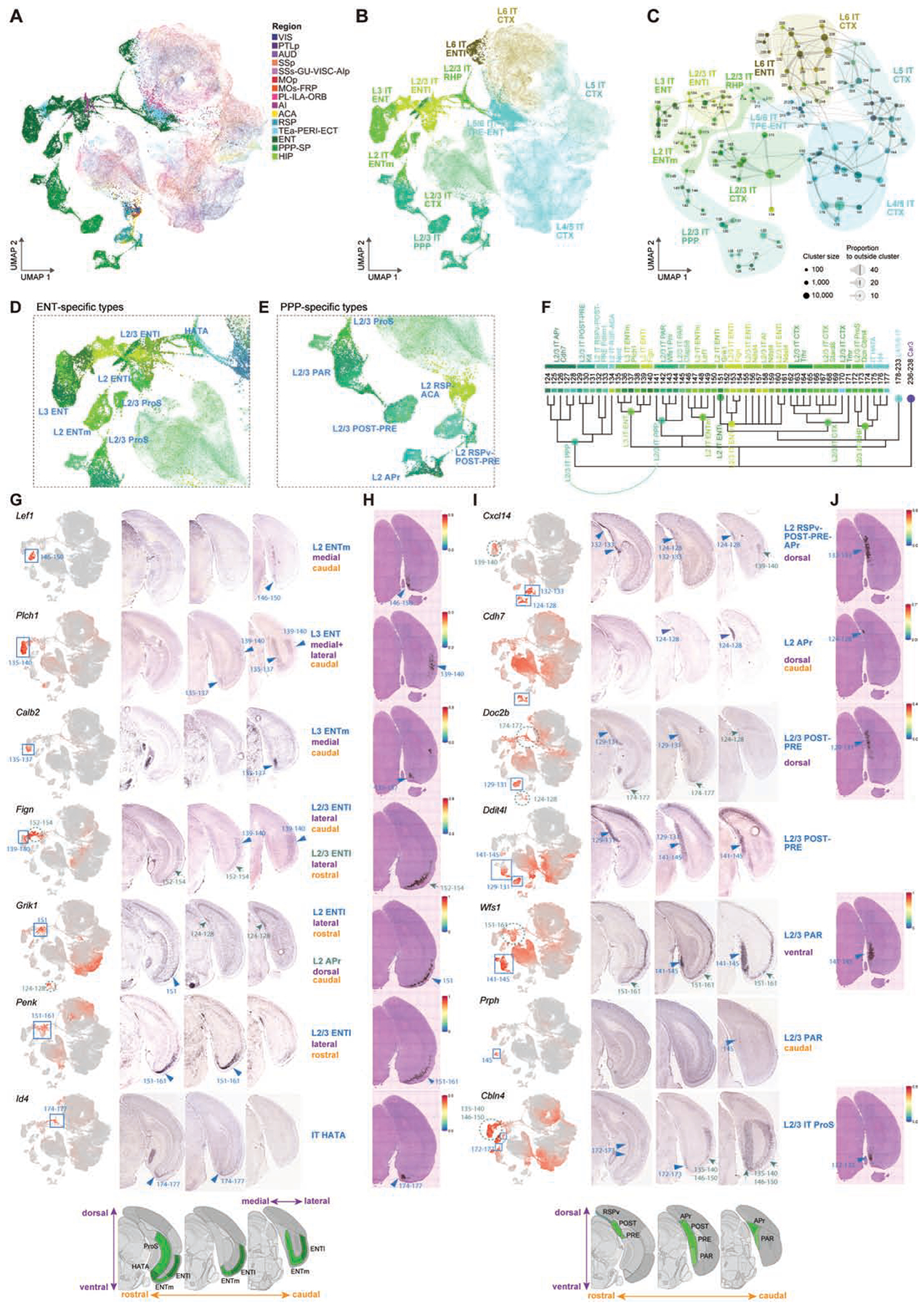
(A-B) UMAP representation of IT neurons from CTX and HPF, colored by region (A) or subclass (B). The CTX neurons are faded out.

(C) Constellation plot of IT types from CTX and HPF. Clusters are grouped by subclass.

(D-E) Enlarged view of UMAP in B of ENT- (D) or PPP-specific (E) types colored by cluster.

(F) Dendrogram of CTX, ENT and PPP IT clusters with branches annotated by subclass and supertype.

(G) Anatomical annotation of various supertypes marked in D. UMAP representations, as in B, show expression of select supertype marker genes in red (blue boxes). RNA ISH images of supertype markers along three rostral to caudal sections reveal specific locations of the different supertypes (blue arrowheads). Green dashed circles and green arrows show additional expression sites of markers.

(H) Spatial verification of supertypes shown in G using Visium. Spatial RNA-seq barcoded spots are labeled by prediction score for specified supertype.

(I-J) Same as G-H but for supertypes marked in E.

The ENT IT group (Fig. 4B–D, F–H) has 10 supertypes organized in a layer-selective manner, in the order of L2, L2/3, L3, L5 and L6, consistent with their correspondence with CTX L2/3-L6 IT types, and shows differential spatial distribution along the anterior-posterior axis, as shown by marker gene ISH and the Visium spatial transcriptomics platform (Fig. 4G–H). The L3 IT ENT subclass is found in the caudal part, including the Plch1 supertype specific to ENTm and the Fign supertype specific to ENTl. The Penk+ L2/3 IT ENTl subclass, including the Fign and Ndst4 supertypes, sits in the rostral ENTl. Two supertypes, L2 IT ENTm Lef1 and L2 IT ENTl Chn2 (Grik1+), are located at the border between L1 and L2. The L2/3 RHP subclass contains two supertypes assigned to the superficial layers of ProS (L2/3 IT ProS Dcn Cbln4, Fig. 4I–J) and HATA (IT HATA Id4, also extending to ventral ENT) regions (Ding et al., 2020). The L5/6 IT TPE-ENT Dcn supertype (Rorb+) contains L5/6 cells in ENTl and caudal ventral part of ENTm. The L6 IT ENTl Dlk1 supertype is specifically located in L6 of the rostral and middle ENTl.

The PPP IT group (Fig. 4B–C, E–F, I–J) contains the L2/3 IT PPP subclass and is most closely related to supertype L2 IT RSP-ACA Npnt (cluster #134), consistent with the anatomical proximity of PPP and RSP. The supertypes within L2/3 IT PPP follow a rostral dorsal to caudal ventral transition (Fig. 4E, I–J), starting with the Pdlim1 supertype in L2 of RSPv, POST and PRE, then the Kit supertype in L2/3 of POST-PRE, followed by the Wfs1 Prlr supertype in L2/3 of PAR, and the Cfap58 supertype (#145) in caudal PAR. The Cdh7 supertype is specific to L2 of the APr region.

The NP/CT/L6b neighborhood contains sets of L5/6 NP, L6 CT and L6b subclasses well matched between CTX and HPF (Fig. 5A–D). L5/6 NP CTX is closely related to NP SUB and more distantly related to NP PPP. L6 CT CTX is closely related to CT SUB as well as supertype L6 CT ENT Rasgrf2 Rmst. The L6b CTX subclass also contains cells from ENT, PPP and SUB; these cells are mostly in supertype L6b RHP Nxph4 Cobll1. L6b CTX is also closely related to supertype L6b ENT Cplx3 Cobll1. We observe two parallel continuous transitions between L6 CT and L6b types for both CTX and ENT, and a continuous transition of L6b cells between CTX and all HPF regions (Fig. 5A–C). As with the IT cells (Fig. 4), the CTX L5 NP, L6 CT and L6b clusters are largely shared across cortical areas (Fig. 5A, D, S2), whereas the HPF NP and CT cell types are highly distinct among SUB, ENT and PPP. Multiple marker genes and Visium data confirm the regional specificity of these HPF subclasses and supertypes (Fig. S4A–B).

Figure 5. Parallel sets of NP/CT/L6b and L5 PT related cell types in isocortex and hippocampal formation.

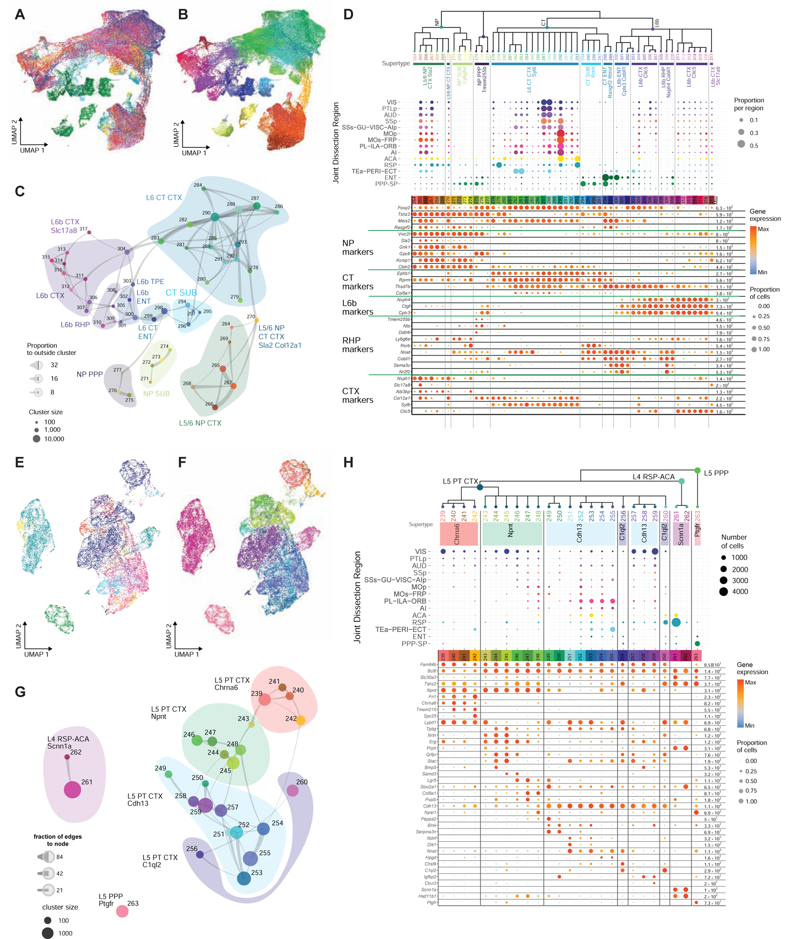
(A-B) UMAP representation of NP/CT/L6b cell types from CTX and HPF, colored by region (A) or cluster (B).

(C) Constellation plot of NP/CT/L6b clusters. Clusters are grouped by supertype.

(D) Dendrogram of NP/CT/L6b clusters followed by dot plots showing proportion of cells within each cluster derived from each region of dissection and marker gene expression in each cluster from the 10xv2 dataset. Clusters are grouped by supertype.

(E-H) Same as A-D but for L5 PT related cell types. Regional dot plot in H shows number of cells per cluster and region.

See also Figure S4.

The PT neighborhood (Bcl6+) is segregated into three region-specific subclasses, L5 PT CTX (Fam84b+), L4 RSP-ACA, and L5 PPP (the only HPF-specific cell type identified in this neighborhood) (Fig. 5E–H). L5 PT CTX contains 4 supertypes: Chrna6 (enriched in posterior sensory areas and highly distinct from the other three supertypes), Npnt, Cdh13 and C1ql2 (enriched in RSP-ACA). The three ALM L5 PT types previously identified (Economo et al., 2018; Tasic et al., 2018) correspond to cluster #248 (thalamus-projecting cells) in the Npnt supertype and clusters #249 and #252 (medulla-projecting cells) in the Cdh13 supertype, respectively (Fig. S4D). It will be interesting to see if cells in other cortical areas belonging to these two supertypes have similarly differential projection patterns. Of note, in the Cdh13 supertype, clusters #251–255 (Nnat+) are mostly populated by cells from prefrontal, medial and lateral associational areas, and #251 is highly specific to PL-ILA and ACA-RSP, based on marker genes Ndnf and Dlk1 (Fig. 5H, S4C).

L4 RSP-ACA Scnn1a is an unusual subclass/supertype. It expresses PT marker gene Bcl6 but not Fam84b; it also expresses a pan-IT marker Slc30a3, as well as L4 IT-specific markers Rspo1 and Scnn1a but not Rorb (Fig. 5H). It is located more superficially than supertype L5 PT C1ql2 in RSP (Fig. S4C). Projection mapping (http://connectivity.brain-map.org/; experiments 166269090, 166458363 and 181860879) (Oh et al., 2014) showed that neurons labeled via Scnn1a-Tg3-Cre driver line in RSP have long-range projections to both intra- and extratelencephalic targets; they project to ACA, RHP regions, contralateral RSP, and anteroventral nucleus (AV) of thalamus (Fig. S4E). The gene expression makeup, layer specificity and projection pattern altogether suggest that L4 RSP-ACA Scnn1a has an IT/PT hybrid identity.

Multidimensional variation of cell type distribution in the hippocampal and subicular regions

In the DG/SUB/CA neighborhood, DG, CA2 and CA3 subclasses are highly distinct, whereas SUB-ProS and CA1-ProS subclasses are more closely related (Fig. 6A–D). In the CA3 subclass, we identify a hilar mossy cell supertype, Mossy Rgs12, based on multiple marker genes including Gal, Rgs12, Glipr1, Necab1 and Calb2 (Scharfman and Myers, 2012) (Data S1, HPF markers).

Figure 6. Multi-dimensional distribution of glutamatergic cell types in hippocampus and subiculum.

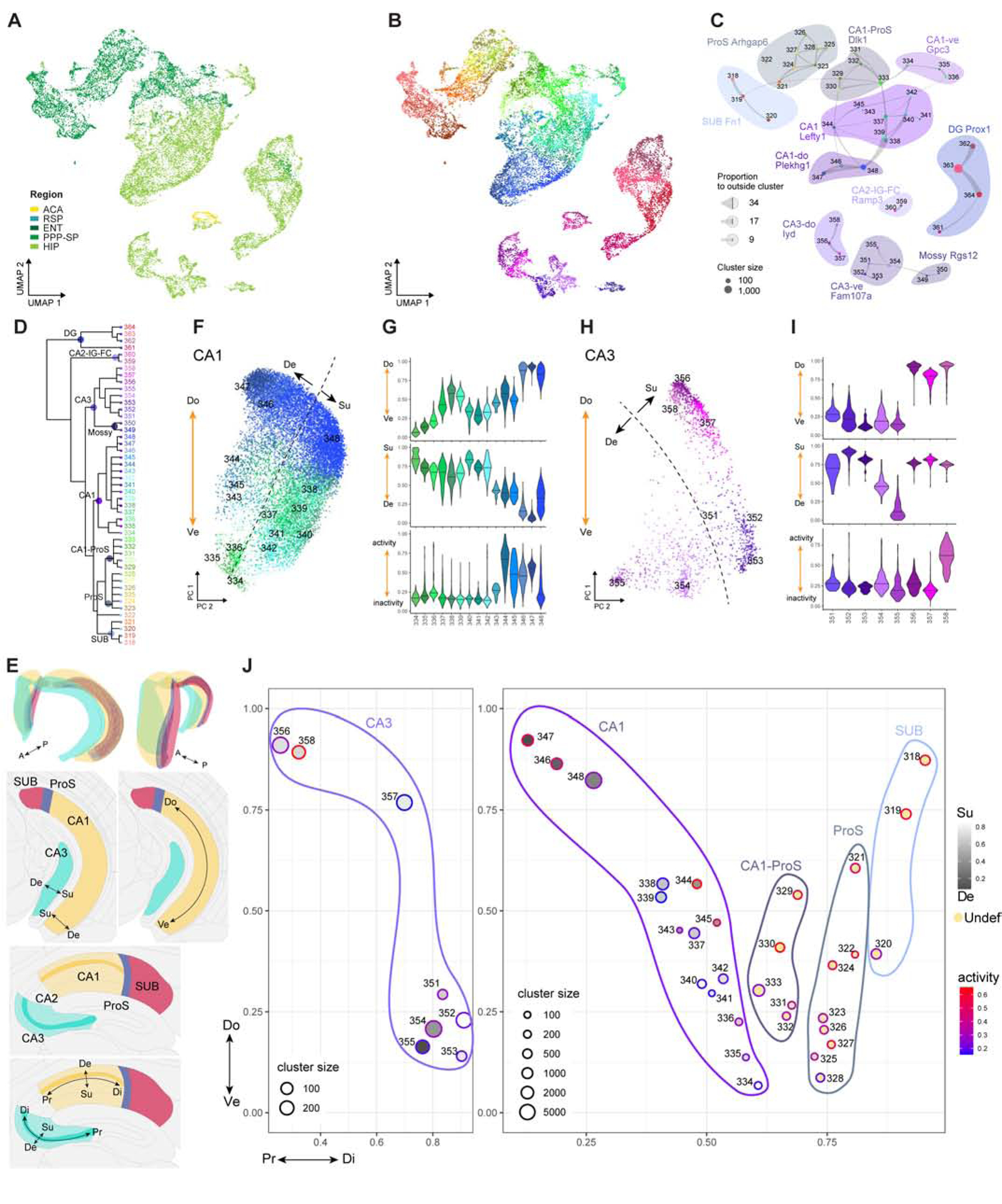
(A-B) UMAP representation of DG/SUB/CA cell types, colored by region (A) or cluster (B).

(C) Constellation plot of DG/SUB/CA clusters. Clusters are grouped by supertype.

(D) Dendrogram of DG/SUB/CA clusters with annotation of major branches.

(E) 3D and 2D schematics showing spatial axes within hippocampus and subiculum: proximal-distal (Pr-Di), superficial-deep (Su-De), and dorsal-ventral (Do-Ve). Images are rendered from CCFv3.

(F) 2D PCA plot for CA1cells. PC1 corresponds to the Do-Ve axis. Dashed line shows the putative Su-De separation.

(G) Violin plots showing distribution of CA1 clusters along Do-Ve, Su-De and activity axes.

(H-I) Same as F-G but for CA3 cells.

(J) Summary of cell type variation in Pr-Di, Do-Ve, Su-De and activity dimensions for CA3, CA1, ProS, and SUB. Each circle represents a cluster, for which the average values for its cell members along each of the four dimensions are computed.

See also Figure S5, Data S1.

The DG subclass, marked by Prox1, has a dominant cluster, #363, which contains vast majority of the granule cells (Fig. S2). We did not find clusters strongly related to adult neurogenesis in DG (Goncalves et al., 2016), indicating that immature neurons or progenitors might not be well labeled by the pan-neuronal or pan-glutamatergic Cre lines we used for this study. The CA2 subclass also contains cells from the small IG and FC regions.

CA1, CA3 and SUB have gradual gene expression and connectivity changes along multiple dimensions – superficial-deep, proximal-distal and dorsal-ventral (Cembrowski and Spruston, 2019). To understand the relationship between all the hippocampal and subicular clusters and the three-dimensional spatial structure of these regions (Fig. 6E), we used UMAP and principal component analysis (PCA) to evaluate the patterns of variation among our CA/SUB cell types and their correlation with previously described dimensions.

We first extracted one main axis that drove CA1, ProS and SUB variation by one dimensional UMAP of all the cells in the CA1-ProS and SUB-ProS subclasses, and found that this axis corresponded to a proximal-distal (Pr-Di) gradient from CA1 to SUB, for which each stage of the transition was driven by a different set of genes (STAR Methods, Fig. S5A–B, Data S1, HPF gradients).

To examine other axes of variation, we performed PCA for CA1 and CA3 (excluding the Mossy Rgs12 supertype) separately and found the top PC corresponded to a dorsal-ventral (Do-Ve) gradient (Fig. 6F–I). We identified a core set of genes that specify this gradient not only in CA1 and CA3 but also in SUB/ProS and DG (STAR Methods), which we hypothesize is the core program for dorsal-ventral gradient specification. The distribution of cells in each cluster from all regions, segregated by subclasses, along this axis is shown along with a subset of genes in the core program (Fig. S5C) and ISH images of selected genes that are dorsal or ventral specific (Fig. S5D, Data S1, HPF gradients).

In both CA1 and CA3, key genes contributing to the second PC corresponded to the superficial-deep (Su-De) radial axis, as validated by RNA ISH images (STAR Methods, Fig. 6F–I, S5G–J, Data S1, HPF gradients). The separation of layer markers is more prominent in the ventral part of CA3 than its dorsal part. In CA1 and CA3, superficial and deep clusters have a weak correlation with L2/3 IT CTX and L5 PT CTX, respectively (Fig. S5G, I).

The Do-Ve distribution of CA1 and CA3 clusters follow the taxonomy branches well (Fig. 6C, F–I). In CA1, supertype CA1-ve Gpc3 (#334–336) is in the most ventral location, followed by CA1 Lefty1 (#337–345), and CA1-do Plekhg1 (#346–348) most dorsal. In CA3, supertype CA3-do Iyd (#356–358) is in the dorsal location, and CA3-ve Fam107a (#351–355) more ventral. In the less diverse parts of CA1 (most ventral) and CA3 (most dorsal), the Su-De distinction is also less obvious; correlated with this, clusters in CA1-ve Gpc3 and CA3-do Iyd are often related to L6 IT CTX (Fig. S5G, I).

Besides Pr-Di, Do-Ve, and Su-De gradients, we also observed an activity-dependent transcriptional signature shared in selected clusters across DG/CA3/CA1/ProS/SUB (Fig. 6G, I, S5E–F). It includes many well-established immediate early genes (IEGs) such as Ier5, Arc, Fos, Egr4 and Nr4a1, known to label neuronal ensembles encoding memory traces (Minatohara et al., 2015). We also identified activity-dependent genes co-expressed with IEGs in a cell type-dependent manner. For example, Gadd45b shows highest expression in DG and is known to be required for activity-induced DNA demethylation of genes critical for adult neurogenesis (Ma et al., 2009).

Finally, we plotted the average values for each cluster along all four dimensions of variation together (Fig. 6J). Overall, glutamatergic cell types exhibit gradient distribution in the Do-Ve axis in all hippocampal-subicular regions; CA1, ProS and SUB cell types together form a Pr-Di transition zone; CA1 and CA3 cell types are also distributed along a Su-De division. While there is a large divergence between the dorsal clusters of SUB and CA1 along the Pr-Di axis, there is a convergence in the ventral parts of CA1 and ProS (and HATA). Also notably, the most dorsal clusters in CA1, CA3 and SUB show high levels of activity-dependent gene expression compared to the ventral part, consistent with a previous study of spatial distribution of Arc expression in the hippocampus associated with the differential response to spatial/nonspatial information along the dorsal-ventral axis (Chawla et al., 2018).

Continuous variation of glutamatergic neuron types across layers and regions of isocortex

Here we further investigated observed continuous variations in CTX glutamatergic subclasses. First, we identified a vertical gradual transition of all CTX IT clusters along the cortical depth. UMAP containing the four common CTX IT subclasses (L2/3, L4/5, L5 and L6) revealed a gradual transition of the subclasses from L2/3 to L6 (Fig. S6A). To further define this continuum, we computed one-dimensional UMAP for all the IT cells based on the PCs in imputed space, which corresponded well with cortical depth, and from this we calculated a pseudo-layer dimension and colored the IT UMAP according to this dimension (Fig. S6B). Distribution of cells in each cluster along the pseudo-layer dimension showed that the clusters fall along a gradient (Fig. S6D). Correspondence between the pseudo-layer dimension and actual cortical layers was established by calculating the expression of layer-specific marker genes (e.g., Otof, Rspo1, Fezf2, Osr1) for cells ordered along the pseudo-layer dimension (Fig. S6D–F, Data S1, IT layer markers). Collectively the clusters, and the supertypes and subclasses they belong to, transition continuously across cortical depth from superficial to deep, making the traditional layer separation less clear, especially for the borders between L4 and L5 and between L5 and L6. We identified a L4 specific supertype, L4 IT CTX Rspo1, which predominantly contains cells from all sensory areas but surprisingly, some from non-sensory isocortical areas as well (Fig. S6D). This supertype likely represents the L4 spiny stellate or star pyramid neurons that are morphologically distinct from the pyramidal neurons in other layers (Harris and Shepherd, 2015), however, it’s worth noting that transcriptomically this type is continuous with the L4/5 IT cells (Fig. S6A–D).

Next, we examined regional distribution specificity of all CTX glutamatergic subclasses (IT, PT, NP, CT and L6b). Nearly all clusters in these subclasses contain cells from multiple isocortical areas (Fig. S2). Although enrichment in specific areas is seen for some clusters, there is rarely one-to-one correspondence between clusters and regions. To further investigate cross-area variations, we created a separate UMAP for each subclass (Fig. 7A), excluding cell types with strong regional specificity (e.g., L4 RSP-ACA Scnn1a, L5 PT Chrna6, and transitional types to HPF). In almost all cases, the medial (RSP/ACA) and lateral (TEa-PERI-ECT, collectively TPE) regions are more distinct while the anterior-to-posterior transition is more continuous. Individual clusters within each subclass occupy specific domains on the gradient map, with more similar clusters located closer to each other (Fig. S7), in agreement with the existence of modules along the cortical sheet (Harris et al., 2019).

Figure 7. Regional gradients of distribution of glutamatergic cell types in isocortex.

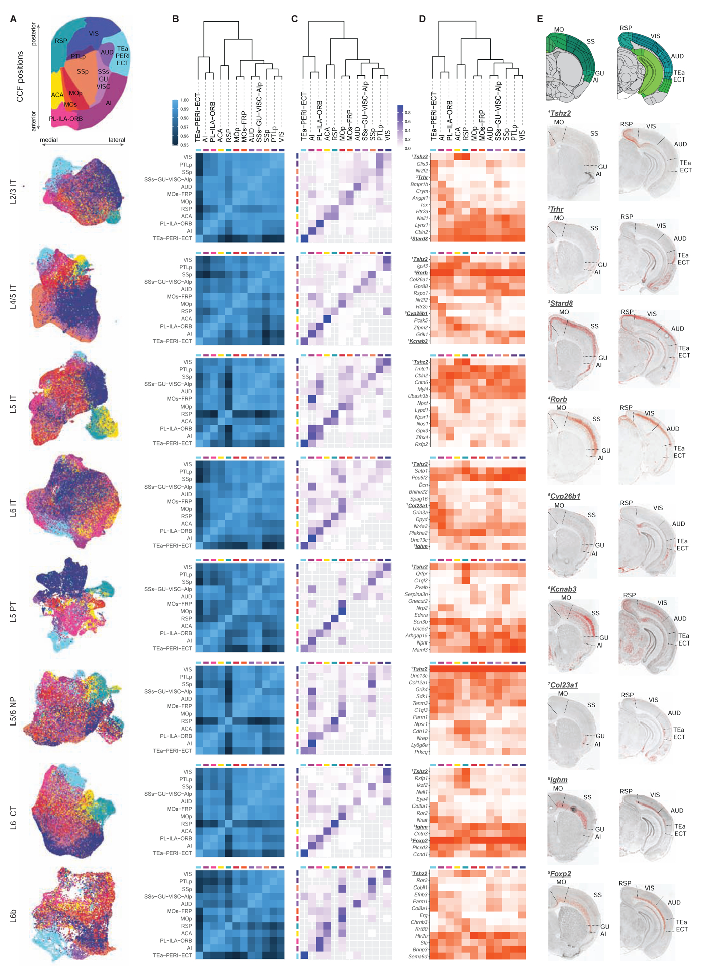
(A) UMAP plots of isocortical cells in different subclasses. At the top is a 2D flatmap representation of isocortical regions according to their positions in CCFv3.

(B) Heatmap of correlation between cortical regions for each subclass. At the top of B-D is a dendrogram of cortical regions generated based on their average gene expression within each subclass and concatenated across all subclasses.

(C) Confusion matrix of the predictability of cortical regions for each subclass. Rows and columns correspond to the actual and predicted regional identities of cells, with the rows adding up to 1.

(D) Heatmap of region-specific marker genes for each subclass. Color corresponds to fraction of cells expressing the given gene in each region.

(E) RNA ISH images for numbered genes in D, showing regional distribution of marker gene expression for specific subclasses.

See also Figures S6–S8, Data S1.

To assess the global relationship among isocortical regions, we built a dendrogram based on their average gene expression profiles within each subclass, concatenated across all subclasses (Fig. 7B). We observe the following grouping based on the tree: lateral and prefrontal areas TPE/AI/PL-ILA-ORB, medial areas RSP/ACA, motor areas MOp and MOs, then all the sensory areas AUD, SSp, SSs-GU-VISC, PTLp and VIS. The pairwise correlation heatmaps of all areas for each subclass reveal consistent patterns with the tree, and again showing TPE and RSP as the most distinct areas (Fig. 7B). Next, we assessed separability of different cortical areas based on their transcriptomes (Fig. 7C, STAR Methods). In most cases, cells were preferentially predicted to belong to the region they were dissected from, particularly for the medial, lateral, and prefrontal areas. There is very little confusion between regions that are distant, whereas considerable confusion exists between neighboring regions, particularly for sensory areas. Region separation is more distinct for L5 PT and L4/5 IT than for other subclasses. We also identified key transcriptional signatures that contribute to regional diversity (Fig. 7D–E).

Finally, we extended the analysis of activity-dependent clusters described in HPF to all regions (Fig. S8A–C) and identified a few highly activated clusters in L2/3 IT, L6 IT and L6 CT subclasses. Particularly, supertype L2/3 IT CTX Baz1a (cluster #171) is a strongly activated cluster and likely corresponds to a subset of cortical L2/3 neurons that express IEG c-fos under basal conditions and are preferentially interconnected within the L2/3 network (Yassin et al., 2010). We also characterized the distribution of activity gradient among different cortical areas within each subclass (Fig S8D). Visual areas (VIS and PTLp) have higher fractions of activated cells than other regions, particularly in L2/3 IT subclass, possibly due to their response to light. On the other hand, the TPE region has a consistent depletion of activated cells across all subclasses. L5/6 NP and GABAergic cells appear much less activated and show little regional difference.

DISCUSSION

In this study, we present a comprehensive taxonomy of transcriptomic cell types across the adult mouse isocortex and hippocampal formation (Fig. 1, 3). Major findings regarding neuronal cell type organization within these two brain structures can be summarized as follows.

• 1At transcriptomic level, cell types can be organized in a hierarchical manner over a complex landscape with both discrete and continuous variations. Such molecular relationships correlate strongly with the spatial arrangement (both location and layer) of the cell types.
• 2Glutamatergic neuron types are more diverse than GABAergic neuron types, both molecularly and spatially. We define 28 subclasses, 56 supertypes and 241 types/clusters in the glutamatergic class and 6 subclasses, 30 supertypes and 119 types/clusters in the GABAergic class. In both classes, some cell types are highly specific to a region, layer or location, while others are widely distributed and shared among multiple regions.
• 3Extending from our previous study (Tasic et al., 2018), we find that GABAergic neuron types are shared among all isocortical areas and HPF. We also identify an additional set of GABAergic types that are specific to HPF (Fig. 2). Our current CTX-HPF GABAergic taxonomy corresponds well with previous transcriptomic and multimodal studies from individual regions; the correspondence is the most robust at supertype level (Fig. S1). The identification of both shared and HPF-specific GABAergic types will facilitate comparative studies between HPF and isocortical GABAergic neurons and bridge the vast literature for both, as these neurons from the two regions often have substantially different morphological and connectional patterns and, without transcriptomic classification, it had been difficult to establish the precise correspondence between them (Fishell and Rudy, 2011; Pelkey et al., 2017).
• 4Across all isocortical areas, most glutamatergic cell types are shared among multiple areas (Fig. 3B, S2), contrary to what we found in our previous study of two distantly located cortical areas, VISp and ALM (Tasic et al., 2018). This difference is reconciled by our finding that these transcriptomic cell types are distributed in a continuous and graded manner across cortical sheet, often along anterior-posterior (more continuous) and medial-lateral (more discrete) dimensions (Fig. 7). In addition, isocortical IT neuron types are continuously distributed across the entire cortical depth, from L2/3 to L6 (Fig. S6). Furthermore, glutamatergic cell types in subiculum (SUB) and different fields of hippocampus (HIP) exhibit simultaneous continuous variation in three dimensions – proximal-distal, dorsal-ventral and superficial-deep (Fig. 6). Thus, continuous gradient-like distribution of closely related cell types in various spatial dimensions appears to be a widely applicable rule.

Many previous studies had shown the existence of continuous or discrete subdivisions along the said axes in HIP and SUB (Bienkowski et al., 2018; Cembrowski and Spruston, 2019; Ding et al., 2020; Thompson et al., 2008). However, since these variations in multiple dimensions are intermingled in the convoluted hippocampal and subicular structures, in the absence of comprehensive and systematic transcriptomic data it had been impossible to tease out the exact pattern of these variations. Here, we computationally extracted large sets of genes associated with the principal components (PCs) of the variations across cell types. Using the in situ expression patterns of these genes, the correspondence between these PCs and spatial dimensions or anatomical locations emerges and allows for deriving a more complete picture of the multidimensional variation of gene expression and cell type distribution all at once (Fig. 6, S5).

• 5We find a small number of isocortical glutamatergic cell types that are specific to one or two regions (Fig. 3B), mostly to anterior cingulate (ACA) and retrosplenial (RSP) areas. We also identify cell types that are shared between ventral RSP and post- and presubiculum (POST-PRE), and between lateral associational cortical areas and entorhinal cortex (ENT), suggesting relatedness of these regions. The combination of these region-specific cell types and the continuous variation of shared cell types across isocortical areas collectively defines cortical areal modularity (Fig. 3B, 7), providing a molecular basis for the cortical modularity revealed in connectivity and brain imaging studies (Harris et al., 2019).
• 6We discover a parallel organization of homologous sets of glutamatergic neuron types between HPF and isocortex, revealing the complexity of cell type composition in HPF (Fig. 3, S3). The superficial (and deep) layers of lateral and medial ENT and POST-PRE-PAR (PPP), as well as smaller regions ProS, HATA and APr, resemble the superficial (and deep) layers of isocortex with parallel sets of IT types (Fig. 4). The deep layers of ENT and PPP, as well as SUB, resemble the deep layers of isocortex with parallel sets of NP/CT/L6b types (Fig. 5). Surprisingly, ENT and PPP do not have major cell types resembling L5 PT, which are the major output projection neuron types from isocortex to subcortical regions, except for a single cluster (L5 PPP, #263) (Fig. 5). Instead, we find that majority of the cell types in SUB, ProS and CA1 are homologous to isocortical PT cells (Fig. 3A), suggesting that these cell types may be the major HPF output projection neurons to other cortical and subcortical regions. Therefore, we can find homologous cell types in HPF for all subclasses of isocortical glutamatergic neurons (Fig. 3). These homologous relationships are supported by similar expression patterns of a large set of marker genes including canonical isocortical subclass-specific transcription factors (Fig. S3), and similar laminar localization as demonstrated by ISH and Visium data, between corresponding pairs of IT/NP/CT/L6b cell types. For SUB/ProS/CA1 cell types and isocortical L5 PT cells, even though they do not have similar layer specificity, their homology is supported by the co-expression of at least five L5 PT defining transcription factors in SUB/ProS/CA1 cell types (Fig. S3).

These homologous relationships raise the intriguing possibility that the axon projection patterns of the HPF glutamatergic types may follow similar rules for those of isocortical neurons (e.g., corticocortical, subcerebral/corticofugal, corticothalamic, or local/near projections for IT, PT, CT or NP subclasses, respectively). Thus the transcriptomic cell type-based molecular architecture of HPF predicts an isocortex-like circuit organization, with IT-like projections from superficial (and deep) layers of ENT and PPP to other HPF regions (including HIP) and within HIP from DG to CA3 to CA1, output projections from PT-like CA1, ProS and SUB going out of HPF to widespread cortical and subcortical targets, and additional output projections from CT-like cells from deep layers of ENT, PPP and SUB to thalamus or related regions. This prediction is highly consistent with the currently known interareal connections of HPF, providing a level of validation to the transcriptomic cell type framework (Bienkowski et al., 2018; Ding et al., 2020; Gergues et al., 2020; van Strien et al., 2009). For example, it has been shown that superficial neurons in SUB mainly project within HPF whereas its deep-layer neurons have subiculo-fugal or subiculo-thalamic projections (Bienkowski et al., 2018). A major implication of this is that we can now begin to dissect the interareal connections at transcriptomic cell type level and build a cell type-based comprehensive wiring diagram of this highly complex circuit.

The glutamatergic neurons in HPF across the dorsal-ventral axis display differential cellular properties and connectivity patterns, and have been associated with different behavioral roles (Cembrowski and Spruston, 2019). A prominent function of the hippocampal formation is spatial navigation, with a number of functionally specific cell types identified in various HPF regions, such as grid cells in ENTm, head direction cells in PPP and ENTm, and place cells in CA1 (Moser et al., 2017). Underlying the functions are complex yet highly organized input and output connections across many regions both within and outside HPF (Bienkowski et al., 2018; van Strien et al., 2009). It will be of immense interest to examine the extent to which transcriptomic cell types are the nodes underlying specific connectional pathways and playing specific functional roles. For example, we hypothesize that the Calb1+ L3 IT ENTm Plch1 cells and the Reln+ L2 IT ENTm Lef1 cells may contain the pyramidal and stellate grid cells, respectively, based on the expression of these known grid cell marker genes (Ferrante et al., 2017; Nilssen et al., 2019). In addition, it has been shown that dorsal and ventral parts of the hippocampal-subicular regions form distinct interconnected networks (Bienkowski et al., 2018; Ding et al., 2020). The shared dorsoventral differentially expressed gene sets across these regions identified in our study suggest a common regulatory program for these specific circuits (Fig. S5C).

• 7Finally, the above findings suggest that relationships among cell types revealed by the adult-stage transcriptomic profiles are likely rooted in the developmental and evolutionary processes; consequently, developmental and evolutionary relationships between regions and cell types may also be inferred from transcriptomic cell type relationships.

During embryonic development, isocortical glutamatergic neurons are born within the ventricular and subventricular zones (VZ/SVZ) underneath the cortical plate, which is laid out into a protomap by a gradient or compartmentalized gene expression (Cadwell et al., 2019; O’Leary et al., 2007; Rakic, 1988). In contrast, GABAergic interneurons originate from medial and caudal ganglionic eminences (MGE and CGE, and some from the preoptic area) in the subpallium, and migrate into cortex in tangential streams to populate all cortical regions (Fishell and Rudy, 2011; Hu et al., 2017; Lim et al., 2018). This difference in developmental origins may be the underlying reason for the dichotomy between the extensive regional diversity of glutamatergic types and the sharing of a common set of GABAergic types across isocortical regions, as we previously hypothesized (Tasic et al., 2018).

Hippocampal GABAergic neurons also originate from MGE/CGE like the isocortical ones and follow the same migration streams (Fishell and Rudy, 2011; Pelkey et al., 2017). This may explain our finding that all isocortical GABAergic types are also present in all retrohippocampal regions and most of them are found in HIP as well. It will be interesting to investigate if the HPF-specific GABAergic types arise from a unique developmental program. It has been known that MGE and CGE are not homogeneous but each contains multiple subdomains defined by combinatorial expression of transcription factors; progenitors from different subdomains give rise to different GABAergic types (Hu et al., 2017; Lim et al., 2018). Furthermore, different types can be generated at different temporal stages from the same progenitors. The developmental trajectory of these neurons is also modulated by activity-dependent mechanisms that influence their integration into the specific circuits. Thus, GABAergic interneuron diversity is defined by spatially and temporally precise genetic programming and refined by network interactions.

Similarly, area patterning of isocortex is a multi-faceted developmental process, involving an interplay between intrinsic genetic mechanisms and extrinsic inputs from thalamocortical projections (Cadwell et al., 2019; O’Leary et al., 2007). At the early stage of cortical development, signaling molecules and morphogens secreted from localized patterning centers lead to gradient expression of transcription factors in progenitors in VZ/SVZ, establishing a protomap along the cortical sheet. Subsequent formation of more refined functional areas with sharp boundaries in the isocortex is thought to be mainly driven by thalamocortical inputs and activity-dependent mechanisms. Both processes could shape the repertoire and landscape of adult-stage glutamatergic neuron types in isocortex as seen here.

For glutamatergic types in isocortex, we find a small number of types that are specific to one or two regions, all in associational areas; but most types are shared among several or multiple areas with graded variations (Fig. 3B). Regional variations are not uniform among different subclasses, for example, L5 PT and L4/5 IT types appear more distinct across areas than types in other subclasses, and different subclasses contain types that are enriched in different areas (Fig. 7). Overall, we find that medial, prefrontal and lateral associational areas are more distinct from sensorimotor areas and from each other; sensorimotor areas are more continuous but several domains (posterior sensory, lateral sensory and frontal motor) can be discerned. If considering all glutamatergic types together, it is possible to distinguish each area from all other areas (Fig. 7). Thus, the uniqueness of each region can be defined by combining all glutamatergic types together, even though individual types often are not confined to single areas. It should also be noted that our transcriptomic types are defined by unsupervised clustering based on overall gene expression variation, there might be region-specific gene signatures existing in our datasets but not strong enough to drive clustering results. It is also possible that the variation of relative proportions of cells within a given type contributes to regional specificity (Fig. S2).

The hierarchical organization and degree of distinction between glutamatergic types may reflect the evolutionary distance between cell types and the regions they are embedded in, similar to comparison of cortical cell types across vertebrate species (Tosches and Laurent, 2019). Glutamatergic types in different HPF regions are highly distinct from each other and from those in isocortex, consistent with the notion of a more ancient emergence of HPF and its subregions. Interestingly, we find that all major glutamatergic subclasses in isocortex (i.e., L2/3-L6 IT, L5 PT, L5/6 NP, L6 CT and L6b) also exist in various HPF regions. These cell types are components of the integrated HPF circuit that follows similar connectional rules seen in a canonical isocortical circuit. This finding challenges the traditional view that isocortex is newly evolved whereas HPF remains as an older structure during vertebrate evolution (Northcutt and Kaas, 1995; Tosches and Laurent, 2019). Instead, we suggest that both isocortex and HPF in mammals evolved from the simpler three-layered cortex in reptiles into two parallel “six-layered” circuit organizations, while isocortex further went through accelerated evolution resulting in a multiplication of areas each as an independent circuit unit.

In conclusion, our current study establishes a blueprint of the molecular architecture that potentially reflects the developmental/evolutionary origins as well as the connectional/functional specificity of isocortex and hippocampal formation and their subregions. This work also provides the roadmap to genetically target the numerous cell types discovered and categorized here, and lays the foundation for systematic, cell type-specific investigation of the structure and function of these brain circuits.

Limitations of the Study

In this study we assigned anatomical locations of major cell types (mostly at the supertype level) using existing RNA ISH data from the Allen Mouse Brain Atlas and a limited Visium dataset; we also provided an estimate of the relative proportions of different cell types in each region using the 10xv2 data. However, the precise spatial distribution and relative proportion of various cell types should ultimately be established through more comprehensive spatially resolved transcriptomic studies using approaches such as multiplexed FISH, in situ sequencing, or in situ capture followed by sequencing (Close et al., 2021; Larsson et al., 2021; Zhuang, 2021).

STAR METHODS

RESOURCE AVAILABILITY

Lead Contact

Requests for further information should be directed to and will be fulfilled by the Lead Contact, Hongkui Zeng (hongkuiz@alleninstitute.org).

Materials Availability

Transgenic mouse lines and viral vectors used in this study are available from The Jackson Laboratory, MMRRC or Allen Institute for Brain Science as indicated in the above Key Resources Table.

KEY RESOURCES TABLE

REAGENT or RESOURCE	SOURCE	IDENTIFIER
Bacterial and Virus Strains
rAAV2-retro-EF1a-Cre	Tervo et al., 2016; Allen Institute Viral Core	N/A
rAAV2-retro-CAG-GFP	Tervo et al., 2016	N/A
rAAV2-retro-CAG-tdTomato	Tervo et al., 2016	N/A
rAAV2-retro-EF1a-dTomato	Tervo et al., 2016; Allen Institute Viral Core	N/A
RVΔGL-Cre	Chatterjee et al., 2018; from the lab of Ian Wickersham	N/A
CAV-Cre	Hnasko et al., 2006; from the lab of Miguel Chillon Rodrigues	N/A
rAAV-mscRE4-minBGpromoter-FlpO-WPRE3	Graybuck et al., 2021; Allen Institute Viral Core	N/A
rAAV-mscRE10-minBGpromoter-FlpO-WPRE3	Graybuck et al., 2021; Allen Institute Viral Core	N/A
rAAV-mscRE16-minBGpromoter-FlpO-WPRE3	Graybuck et al., 2021; Allen Institute Viral Core	N/A
Chemicals, Peptides, and Recombinant Proteins
Trimethoprim (TMP)	Sigma-Aldrich	T7883-5G
Tamoxifen (TAM)	Sigma-Aldrich	T5648-5G
Critical Commercial Assays
SMART-Seq v4 Ultra Low Input RNA Kit for Sequencing	Takara	634894
Nextera XT Index Kit V2 Set A-D	Illumina	FC-131-2001, FC-131-2002, FC-131-2003, FC-131-2004
Chromium Single Cell 3’ Reagent Kit v2	10x Genomics	120237
Deposited Data
Transcriptomic data – fastq files	This paper; NeMO	https://assets.nemoarchive.org/dat-jb2f34y
Transcriptomic data – SMART-seq processed count file and sample metadata	This paper; Allen Institute for Brain Science; NeMO	https://portal.brain-map.org/atlases-and-data/rnaseq/mouse-whole-cortex-and-hippocampus-smart-seq; https://assets.nemoarchive.org/dat-jb2f34y
Transcriptomic data – 10x processed count file and sample metadata	This paper; Allen Institute for Brain Science; NeMO	https://portal.brain-map.org/atlases-and-data/rnaseq/mouse-whole-cortex-and-hippocampus-10x; https://assets.nemoarchive.org/dat-jb2f34y
Cell type cards website that provides specific information for each cell type: markers, cell type metadata, correspondence with cell types in previous publications and relation to neighboring cell types	This paper; Allen Institute for Brain Science	https://taxonomy.shinyapps.io/ctx_hip_browser_v2/
Experimental Models: Organisms/Strains
Mouse: B6.Cg-Gt(ROSA)26Sortm14(CAG-tdTomato)Hze/J, Ai14(RCL-tdT)	The Jackson Laboratory	RRID: IMSR_JAX:007914
Mouse: B6;129S-Gt(ROSA)26Sortm65.1(CAG-tdTomato)Hze/J, Ai65(RCFL-tdT)	The Jackson Laboratory	RRID: IMSR_JAX:021875
Mouse: B6;129S-Gt(ROSA)26Sortm66.1(CAG-tdTomato)Hze/J, Ai66(RCRL-tdT)	The Jackson Laboratory	RRID: IMSR_JAX:021876
Mouse: Ai65F(RCF-tdT)	Daigle et al., 2018	N/A
Mouse: Ai110(RCL-FnGF-nT)	Daigle et al., 2018	N/A
Mouse: B6.Cg-Gt(ROSA)26Sortm75.1(CAG-tdTomato*)Hze/J, Ai75(RCL-nT)	The Jackson Laboratory	RRID: IMSR_JAX:025106
Mouse: B6.Cg-Igs7tm140.1(tetO-EGFP,CAG-tTA2)Hze/J, Ai140(TIT2L-GFP-ICL-tTA2)	The Jackson Laboratory	RRID: IMSR_JAX:030220
Mouse: B6.Cg-Igs7tm148.1(tetO-GCaMP6f,CAG-tTA2)Hze/J, Ai148(TIT2L-GC6f-ICL-tTA2)	The Jackson Laboratory	RRID: IMSR_JAX:030328
Mouse: B6.Cg-Snap25tm1.1Hze/J, Snap25-LSL-F2A-GFP	The Jackson Laboratory	RRID: IMSR_JAX:021879
Mouse: B6.Cg-Calb1tm2.1(cre)Hze/J, Calb1-IRES2-Cre	The Jackson Laboratory	RRID: IMSR_JAX:028532
Mouse: B6(Cg)-Calb2tm1(cre)Zjh/J, Calb2-IRES-Cre	The Jackson Laboratory	RRID: IMSR_JAX:010774
Mouse: STOCK Ccktm1.1(cre)Zjh/J, Cck-IRES-Cre	The Jackson Laboratory	RRID: IMSR_JAX:012706
Mouse: B6;129S6-Chattm2(cre)Lowl/J, Chat-IRES-Cre	The Jackson Laboratory	RRID: IMSR_JAX:006410
Mouse: STOCK Tg(Chrna2-cre)OE25Gsat/Mmucd, Chrna2-Cre_OE25	MMRRC	RRID: MMRRC_036502-UCD
Mouse: STOCK Tg(Chrnb3-cre)SM93Gsat/Mmucd, Chrnb3-Cre_SM93	MMRRC	RRID: MMRRC_036469-UCD
Mouse: B6(Cg)-Crhtm1(cre)Zjh/J, Crh-IRES-Cre_ZJH	The Jackson Laboratory	RRID: IMSR_JAX:012704
Mouse: B6.Cg-Ccn2tm1.1(folA/cre)Hze/J, Ctgf-T2A-dgCre	The Jackson Laboratory	RRID: IMSR_JAX:028535
Mouse: B6(Cg)-Cux2tm3.1(cre/ERT2)Mull/Mmmh, Cux2-CreERT2	MMRRC	RRID: MMRRC_032779-MU
Mouse: B6;129S-Esr2tm1.1(cre)Hze/J, Esr2-IRES2-Cre	The Jackson Laboratory	RRID: IMSR_JAX:030158
Mouse: B6(Cg)-Etv1tm1.1(cre/ERT2)Zjh/J, Etv1-CreERT2	The Jackson Laboratory	RRID: IMSR_JAX:013048
Mouse: B6J.Cg-Gad2tm2(cre)Zjh/MwarJ, Gad2-IRES-Cre	The Jackson Laboratory	RRID: IMSR_JAX:028867
Mouse: STOCK Tg(Colgalt2-cre)NF107Gsat/Mmucd, Glt25d2-Cre_NF107	MMRRC	RRID: MMRRC_036504-UCD
Mouse: B6.Cg-Gnb4tm1.1(cre/ERT2)Hze/J, Gnb4-IRES2-CreERT2	The Jackson Laboratory	RRID: IMSR_JAX:030159
Mouse: Tg(Gng7-cre)KH71Gsat, Gng7-Cre_KH71	Gerfen et al., 2013; from the lab of Charles Gerfen	MGI:4367014
Mouse: STOCK Tg(Htr3a-cre)NO152Gsat/Mmucd, Htr3a-Cre_NO152	MMRRC	RRID: MMRRC_036680-UCD
Mouse: B6.Cg-Ndnftm1.1(folA/cre)Hze/J, Ndnf-IRES2-dgCre	The Jackson Laboratory	RRID: IMSR_JAX:028536
Mouse: STOCK Nkx2-1tm1.1(cre/ERT2)Zjh/J, Nkx2.1-CreERT2	The Jackson Laboratory	RRID: IMSR_JAX:014552
Mouse: B6;129S-Nos1tm1.1(cre/ERT2)Zjh/J, Nos1-CreERT2	The Jackson Laboratory	RRID: IMSR_JAX:014541
Mouse: B6;129S-Npr3tm1.1(cre)Hze/J, Npr3-IRES2-Cre	The Jackson Laboratory	RRID: IMSR_JAX:031333
Mouse: B6.Cg-Npytm1.1(flpo)Hze/J, Npy-IRES2-FlpO	The Jackson Laboratory	RRID: IMSR_JAX:030211
Mouse: FVB-Tg(Nr5a1-cre)2Lowl/J, Nr5a1-Cre	The Jackson Laboratory	RRID: IMSR_JAX:006364
Mouse: B6.FVB(Cg)-Tg(Ntsr1-cre)GN220Gsat/Mmucd, Ntsr1-Cre_GN220	MMRRC	RRID: MMRRC_030648-UCD
Mouse: B6;129S-Oxtrtm1.1(cre)Hze/J, Oxtr-T2A-Cre	The Jackson Laboratory	RRID: IMSR_JAX:031303
Mouse: B6;129S-Pdyntm1.1(cre/ERT2)Hze/J, Pdyn-T2A-CreERT2	The Jackson Laboratory	RRID: IMSR_JAX:030197
Mouse: B6;129S-Penktm2(cre)Hze/J, Penk-IRES2-Cre-neo	The Jackson Laboratory	RRID: IMSR_JAX:025112
Mouse: B6.Cg-Pvalbtm3.1(dreo)Hze/J, Pvalb-T2A-Dre	The Jackson Laboratory	RRID: IMSR_JAX:021190
Mouse: B6.Cg-Pvalbtm4.1(flpo)Hze/J, Pvalb-T2A-FlpO	The Jackson Laboratory	RRID: IMSR_JAX:022730
Mouse: B6;129P2-Pvalbtm1(cre)Arbr/J, Pvalb-IRES-Cre	The Jackson Laboratory	RRID: IMSR_JAX:008069
Mouse: B6.Cg-Rasgrf2tm2.1(folA/flpo)Hze/J, Rasgrf2-T2A-dgFlpO	The Jackson Laboratory	RRID: IMSR_JAX:029589
Mouse: STOCK Tg(Rbp4-cre)KL100Gsat/Mmucd, Rbp4-Cre_KL100	MMRRC	RRID: MMRRC_031125-UCD
Mouse: B6;129S-Rorbtm1.1(cre)Hze/J, Rorb-IRES2-Cre	The Jackson Laboratory	RRID: IMSR_JAX:023526
Mouse: B6.Cg-Rorbtm3.1(flpo)Hze/J, Rorb-IRES2-FlpO	The Jackson Laboratory	RRID: IMSR_JAX:029590
Mouse: Rorb-P2A-FlpO	Daigle et al., 2018	N/A
Mouse: B6;C3-Tg(Scnn1a-cre)2Aibs/J, Scnn1a-Tg2-Cre	The Jackson Laboratory	RRID: IMSR_JAX:009112
Mouse: B6;C3-Tg(Scnn1a-cre)3Aibs/J, Scnn1a-Tg3-Cre	The Jackson Laboratory	RRID: IMSR_JAX:009613
Mouse: STOCK Tg(Sim1-cre)KJ18Gsat/Mmucd, Sim1-Cre_KJ18	MMRRC	RRID: MMRRC_031742-UCD
Mouse: B6J.129S6(FVB)-Slc17a6tm2(cre)Lowl/MwarJ, Slc17a6-IRES-Cre	The Jackson Laboratory	RRID: IMSR_JAX:028863
Mouse: B6;129S-Slc17a7tm1.1(cre)Hze/J, Slc17a7-IRES2-Cre	The Jackson Laboratory	RRID: IMSR_JAX:023527
Mouse: STOCK Tg(Slc17a8-icre)1Edw/SealJ, Slc17a8-iCre	The Jackson Laboratory	RRID: IMSR_JAX:018147
Mouse: B6;129S-Slc17a8tm1.1(cre)Hze/J, Slc17a8-IRES2-Cre	The Jackson Laboratory	RRID: IMSR_JAX:028534
Mouse: B6J.129S6(FVB)-Slc32a1tm2(cre)Lowl/MwarJ, Slc32a1-IRES-Cre	The Jackson Laboratory	RRID: IMSR_JAX:028862
Mouse: B6.Cg-Slc32a1tm1.1(flpo)Hze/J, Slc32a1-IRES2-FlpO	The Jackson Laboratory	RRID: IMSR_JAX:031331
Mouse: B6.Cg-Slc32a1tm1.1(flpo)Hze/J, Slc32a1-T2A-FlpO	The Jackson Laboratory	RRID: IMSR_JAX:029591
Mouse: B6;129S-Snap25tm2.1(cre)Hze/J, Snap25-IRES2-Cre	The Jackson Laboratory	RRID: IMSR_JAX:023525
Mouse: B6J.Cg-Ssttm2.1(cre)Zjh/MwarJ, Sst-IRES-Cre	The Jackson Laboratory	RRID: IMSR_JAX:028864
Mouse: B6J.Cg-Ssttm3.1(flpo)Zjh/AreckJ, Sst-IRES-FlpO	The Jackson Laboratory	RRID: IMSR_JAX:031629
Mouse: B6;129S-Tac1tm1.1(cre)Hze/J, Tac1-IRES2-Cre	The Jackson Laboratory	RRID: IMSR_JAX:021877
Mouse: B6.FVB(Cg)-Tg(Th-cre)FI172Gsat/Mmucd, Th-Cre_FI172	MMRRC	RRID: MMRRC_031029-UCD
Mouse: C57BL/6N-Thtm1Awar/Mmmh, Th-P2A-FlpO or TH-2A-Flpo	Poulin et al., 2018; MMRRC	RRID: MMRRC_050618-MU
Mouse: B6.FVB(Cg)-Tg(Tlx3-cre)PL56Gsat/Mmucd, Tlx3-Cre_PL56	MMRRC	RRID: MMRRC_041158-UCD
Mouse: B6.Cg-Trib2tm1.1(cre/ERT2)Hze/J, Trib2-F2A-CreERT2	The Jackson Laboratory	RRID: IMSR_JAX:022865
Mouse: B6J.Cg-Viptm1(cre)Zjh/AreckJ, Vip-IRES-Cre	The Jackson Laboratory	RRID: IMSR_JAX:031628
Mouse: STOCK Viptm2.1(flpo)Zjh/J, Vip-IRES-FlpO	The Jackson Laboratory	RRID: IMSR_JAX:028578
Mouse: B6;129S-Vipr2tm1.1(cre)Hze/J, Vipr2-IRES2-Cre	The Jackson Laboratory	RRID: IMSR_JAX:031332
Mouse: STOCK Tg(Gad1-EGFP)98Agmo/J, Gad67-GFP_X98	The Jackson Laboratory	RRID: IMSR_JAX:006340
Software and Algorithms
STAR 2.5.3	Dobin et al., 2013	https://github.com/alexdobin/STAR/releases
CellRanger	10x Genomics	https://support.10xgenomics.com/single-cell-gene-expression/software/downloads/latest
SpaceRanger	10x Genomics	https://support.10xgenomics.com/spatial-gene-expression/software/downloads/latest
scrattch suites for clustering/visualization of single cell dataset that include scrattch.vis, scrattch.hicat, scrattch.bigcat	This paper; Allen Institute for Brain Science	https://github.com/AllenInstitute/scrattch; https://github.com/AllenInstitute/scrattch.vis; https://github.com/AllenInstitute/scrattch.hicat; https://github.com/AllenInstitute/scrattch.bigcat
Seurat v3.4	Stuart et al., 2019	https://github.com/satijalab/seurat
UMAP	McInnes et al., 2018	https://github.com/lmcinnes/umap
R v3.5.0 and greater	R Foundation	https://www.R-project.org
RStudio IDE	RStudio	http://www.rstudio.com

Data and code availability

The raw and processed sequencing data is deposited in the NeMO Archive for the BRAIN Initiative Cell Census Network (https://assets.nemoarchive.org/dat-jb2f34y). Full metadata for all samples are available in Table S2, S3. Transcriptomic data can be visualized and analyzed using the Transcriptomics Explorer at https://portal.brain-map.org/atlases-and-data/rnaseq. We also provide an accompanying website at https://taxonomy.shinyapps.io/ctx_hip_browser_v2/, with a Cell Card for each cell type. The website can be browsed by cell type and provides information on specific markers, cell type metadata, and relation to neighboring cell types.

R packages for the iterative clustering method utilized in this analysis (scrattch.bigcat and scrattch.hicat) are available on GitHub at https://github.com/AllenInstitute/scrattch.hicat, https://github.com/AllenInstitute/scrattch.bigcat.

EXPERIMENTAL MODEL AND SUBJECT DETAILS

Mouse breeding and husbandry

All procedures were carried out in accordance with Institutional Animal Care and Use Committee protocols at the Allen Institute for Brain Science. Animals were provided food and water ad libitum and were maintained on a regular 12-h day/night cycle at no more than five adult animals per cage. Animals were maintained on the C57BL/6J background, and newly received or generated transgenic lines were backcrossed to C57BL/6J. We obtained Gng7-Cre_KH71 (Gerfen et al., 2013) mice from Charles Gerfen and Th-P2A-FlpO (Poulin et al., 2018) mice from Raj Awatramani.

Standard tamoxifen treatment for CreER lines included a single dose of tamoxifen (40 μl of 50 mg ml⁻¹) dissolved in corn oil and administered via oral gavage at postnatal day (P)10–14. Tamoxifen treatment for Nkx2.1-CreERT2;Ai14 was performed at embryonic day (E)17 (oral gavage of the dam at 1 mg per 10 g of body weight), pups were delivered by cesarean section at E19 and then fostered. Cux2-CreERT2;Ai14 mice received tamoxifen treatment at P35 ± 5 for five consecutive days. Trimethoprim was administered to animals containing Ctgf-2A-dgCre by oral gavage at P40 ± 5 for three consecutive days (0.015 ml per g of body weight using 20 mg ml⁻¹ trimethoprim solution). Ndnf-IRES2-dgCre animals did not receive trimethoprim induction, since the baseline dgCre activity (without trimethoprim) was sufficient to label the cells with the Ai14 reporter. We excluded any animals with anophthalmia or microphthalmia.

We used 530 male and female animals to collect 76,381 cells for SSv4 and 54 male and female animals to collect 1,561,952 cells for 10xv2. Animals were euthanized at P53–59 (n = 531), P50–52 (n = 7), and P60–121 (n = 46). No statistical methods were used to predetermine sample size. All donors used in this study are listed in Table S2.

METHOD DETAILS

Retrograde Labeling

We injected rAAV2-retro-EF1a-Cre (Tervo et al., 2016), RVΔGL-Cre (Chatterjee et al., 2018), or CAV-Cre (Hnasko et al., 2006) (gift of Miguel Chillon Rodrigues, Universitat Autònoma de Barcelona) into brains of heterozygous or homozygous Ai14 mice as previously described (Tasic et al., 2016; Tasic et al., 2018). For ALM experiments, we also injected rAAV2-retro-CAG-GFP or rAAV2-retro-CAG-tdTomato (Tervo et al., 2016) into wild-type mice. We injected rAAV2-retro-EF1a-dTomato (Tervo et al., 2016) into Gnb4-IRES2-CreERT2;Ai140 and Cux2-CreERT2;Ai140 (Daigle et al., 2018) mice with the goal of collecting the Car3 cell types. We collected both singly positive (dTomato+) and double-positive (GFP+/dTomato+) cells when possible. We injected rAAV2-retro-EF1a-dTomato into Ctgf-T2A-dgCre;Snap25-LSL-F2A-GFP mice with the goal of collecting L6b projection neurons. Stereotaxic coordinates were obtained from Paxinos adult mouse brain atlas (Supplementary Table 6 in (Tasic et al., 2018)). For two VISp experiments, we injected into SCs by inserting the needle through the cerebellum at a 45°-angle in the posterior to anterior direction. Injection information for each donor is available in Table S2.

Retro-orbital Labeling

We delivered viruses that contain an enhancer element with putative specificity to L5 PT types (rAAV-mscRE4-minBGpromoter-FlpO-WPRE3) and L5 IT and L6 IT types (rAAV-mscRE10-minBGpromoter-FlpO-WPRE3, rAAV-mscRE16-minBGpromoter-FlpO-WPRE3) (Graybuck et al., 2021) into heterozygous or homozygous Ai65F mice into the retroorbital sinus as previously described (Chan et al., 2017). This approach allows the virus to cross the blood-brain barrier for brain-wide delivery of the viral particles. Due to the difficulty of isolating L5 PT neurons, we used this approach to enrich for labeling of specific types for more efficient cell isolation.

Single-cell isolation

We isolated single cells by adapting previously described procedures (Tasic et al., 2018). The brain was dissected, submerged in ACSF, embedded in 2% agarose, and sliced into 250-μm (SMART-Seq) or 350-μm (10x Genomics) coronal sections on a compresstome (Precisionary Instruments). Block-face images were captured during slicing. Regions of interest (ROIs) were then microdissected from the slices and dissociated into single cells with 1 mg/ml pronase (SMART-Seq before 28 June 2018, Sigma P6911–1G) and processed as previously described (Tasic et al., 2018). Fluorescent images of each slice before and after ROI dissection were taken from the dissecting scope. These images were used to document the precise location of the ROIs using annotated coronal plates of CCFv3 as reference (see below).

We used Allen Mouse Brain Common Coordinate Framework version 3 (CCFv3) ontology (http://atlas.brain-map.org/) to define brain regions for profiling and boundaries for dissections. We covered all regions of CTX and HPF and chose sampling at mid-ontology level with judicious joining of neighboring regions (Fig. 1A, Methods S1, Table S1). For tissue dissections, we chose to combine some neighboring regions to avoid microdissections of very small regions and to collect enough cells for profiling, especially for 10xv2. For example, orbital area (ORB) covers ORBl, ORBm and ORBvl, and primary somatosensory area (SSp) covers all SSp subfields. GU-VISC, PL-ILA and TEa-PERI-ECT were combinations of two or three cortical areas, respectively. PAR, POST and PRE were combined into a single dissection region named PPP for SSv4 profiling, and PPP was further combined with SUB and ProS into a joint dissection region named PPP-SP for 10xv2 profiling. Note that manual microdissections are imperfect, but despite the presence of cells from neighboring regions, the dissections still contain substantial enrichment of cells for the targeted regions. In total, for 10xv2, we profiled 12 joint regions for CTX and 3 joint regions for HPF with 30,000–300,000 cells per region; for SSv4, we profiled 17 regions for CTX and 5 regions for HPF with 1,100–14,000 cells per region.

We used transgenic driver lines for fluorescence-positive cell isolation to enrich for neurons, with the vast majority being Cre driver lines crossed to the Ai14-tdTomato reporter (Madisen et al., 2010) (Table S2). A small fraction of SSv4 cells were labeled by retrograde tracing (Retro-seq) or retroorbital injection of AAVs (Table S2). All 10xv2 cells from all regions were isolated from the pan-neuronal Snap25-IRES2-Cre line; Gad2-IRES-Cre line was used to isolate additional GABAergic interneurons from HIP (Methods S1). For SSv4, the transgenic mice used, dissection scheme, and sampling rate varied by regions (Methods S1, Table S2). Our previously published VISp and ALM (part of MOs) SSv4 dataset (~24,000 cells) (Tasic et al., 2018) were also included in the current study; this dataset had utilized a large number of driver lines with either broad or highly specific coverage of different cell types and employed extensive layer-specific dissections. Three other cortical regions, MOp, SSp and ACA, had 5,000–6,600 SSv4 cells each that were also from multiple driver lines and layer-specific dissections. The hippocampal region (HIP), which includes CA1, CA2, CA3, and DG, was divided into four anteroposterior (i.e. dorsoventral) segments, and each segment was profiled using both pan-glutamatergic and pan-GABAergic Cre lines, totaling ~6,600 SSv4 cells. All the other CTX and HPF regions had 1,100–2,000 SSv4 cells each, profiled from pan-glutamatergic and pan-GABAergic Cre lines without layer-specific dissections.

Number of donor animals and proportion of cells contributed by each transgenic line for each cluster are shown in Table S3. Since nearly all clusters are dominated by 10xv2 cells from Snap25-IRES2-Cre mice, and SSv4 cells mainly came from pan-glutamatergic and pan-GABAergic lines with other specialized Cre lines contributing to only a small fraction of cells, the effect of transgenic line variation is minimal. The number of animals contributing to each cluster varies between 2 and 213, with an average of 56 and median of 44. Only 8 clusters had fewer than 4 donor animals each. Thus, individual mouse variability should not affect the cell type identities.

We used mice of both sexes, except that MOp 10xv2 data had only male cells (Methods S1). There were three small, sex specific clusters, #158, #262, #335, all female specific and almost all the cells in these clusters are from highly specific regions in AI, RSP and HIP respectively.

For all 10xv2 samples and for SSv4 samples after 28 June 2018, we improved our protocol with the following changes. Tissue pieces were digested with 30 U/ml papain (Worthington PAP2) in ACSF for 30 minutes at 30°C. Due to the short incubation period in a dry oven, we set the oven temperature to 35°C to compensate for the indirect heat exchange, with a target solution temperature of 30°C. Enzymatic digestion was quenched by exchanging the papain solution three times with quenching buffer (ACSF with 1% FBS and 0.2% BSA). Samples were incubated on ice for 5 minutes before trituration. The tissue pieces in the quenching buffer were triturated through a fire-polished pipette with 600-μm diameter opening approximately 20 times. The tissue pieces were allowed to settle and the supernatant, which now contained suspended single cells, was transferred to a new tube. Fresh quenching buffer was added to the settled tissue pieces, and trituration and supernatant transfer were repeated using 300-μm and 150-μm fire polished pipettes. The single cell suspension was passed through a 70-μm filter into a 15-ml conical tube with 500 ul of high BSA buffer (ACSF with 1% FBS and 1% BSA) at the bottom to help cushion the cells during centrifugation at 100 × g in a swinging bucket centrifuge for 10 minutes. The supernatant was discarded, and the cell pellet was resuspended in the quenching buffer.

All cells were collected by fluorescence-activated cell sorting (FACS, BD Aria II) using a 130-μm nozzle. Cells were prepared for sorting by passing the suspension through a 70-μm filter and adding DAPI (to a final concentration of 2 ng/ml). Sorting strategy was as previously described (Tasic et al., 2018), with most cells collected using the tdTomato-positive label. For SSv4, single cells were sorted into individual wells of 8-well PCR strips containing lysis buffer from the SMART-Seq v4 kit with RNase inhibitor (0.17 U/μl), immediately frozen on dry ice, and stored at −80°C. For 10x Genomics, 30,000 cells were sorted within 10 minutes into a tube containing 500 μl of quenching buffer. We found that sorting more cells into one tube diluted the ACSF in the collection buffer, causing cell death. We also observed decreased cell viability for longer sorts. Each aliquot of sorted 30,000 cells was gently layered on top of 200 μl of high BSA buffer and immediately centrifuged at 230 × g for 10 minutes in a centrifuge with a swinging bucket rotor (the high BSA buffer at the bottom of the tube slows down the cells as they reach the bottom, minimizing cell death). No pellet could be seen with this small number of cells, so we removed the supernatant and left behind 35 μl of buffer, in which we resuspended the cells. The immediate centrifugation and resuspension allowed the cells to be temporarily stored in a high BSA buffer with minimal ACSF dilution. The resuspended cells were stored at 4°C until all samples were collected, usually within 30 minutes. Samples from the same ROI were pooled, cell concentration quantified, and immediately loaded onto the 10x Genomics Chromium controller.

cDNA amplification and library construction

For SSv4 processing, we performed the procedures with positive and negative controls as previously described (Tasic et al., 2018). We used the SMART-Seq v4 Ultra Low Input RNA Kit for Sequencing (Takara Cat# 634894) to reverse transcribe poly(A) RNA and amplify full-length cDNA. We performed reverse transcription and cDNA amplification for 18 PCR cycles (neurons) or 21 PCR cycles (non-neuronal cells) in 8-well strips, in sets of 12–24 strips at a time. All samples proceeded through Nextera XT DNA Library Preparation (Illumina Cat# FC-131–1096) using Nextera XT Index Kit V2 (Illumina Cat# FC-131–2001) and custom index sets (Integrated DNA Technologies). Custom index sets were validated to confirm the same performance as Nextera Index sets before being used on experimental samples. Nextera XT DNA Library prep was performed according to manufacturer’s instructions, with a modification to reduce the volumes of all reagents and cDNA input to 0.4x or 0.5x of the original protocol. Details are available in ‘Documentation’ on the Allen Institute data portal at: http://celltypes.brain-map.org.

For 10xv2 processing, we used Chromium Single Cell 3’ Reagent Kit v2 (10x Genomics Cat# 120237). We followed the manufacturer’s instructions for cell capture, barcoding, reverse transcription, cDNA amplification, and library construction. We targeted sequencing depth of 60,000 reads per cell; the actual median achieved was 59,728 reads per cell across 175 libraries.

Sequencing data processing and QC

Processing of SSv4 libraries was performed as described previously (Tasic et al., 2018). Briefly, libraries were sequenced on an Illumina HiSeq2500 platform (paired-end with read lengths of 50 bp) to a target read depth of 0.5M reads per cell (range 100,275–12,329,698, median 1,003,867). The Illumina sequencing reads were aligned to GRCm38.p3 (mm10) using a RefSeq annotation gff file retrieved from NCBI on 18 January 2016 (https://www.ncbi.nlm.nih.gov/genome/annotation_euk/all/). Sequence alignment was performed using STAR v2.5.3. (Dobin et al., 2013) in the two-pass mode. PCR duplicates were masked and removed using STAR option ‘bamRemoveDuplicates’. Only uniquely aligned reads were used for gene quantification. Gene counts were computed using the R GenomicAlignments package (Lawrence et al., 2013) and summarizeOverlaps function in ‘IntersectionNotEmpty’ mode for exonic and intronic regions separately. For the SSv4 dataset, we only used exonic regions for gene quantification. Cells that met any one of the following criteria were removed: < 100,000 total reads, < 1,000 detected genes (with CPM > 0), < 75% of reads aligned to genome, or CG dinucleotide odds ratio > 0.5. Doublets were removed by first classifying cells into broad classes of excitatory, inhibitory, and non-neuronal based on known markers. Reads that did not map to the genome were then aligned to synthetic constructs (i.e. ERCC) sequences and the E. coli genome (version ASM584v2) and were used as a QC metric.

10xv2 libraries were sequenced on Illumina NovaSeq6000 and sequencing reads were aligned to the mouse pre-mRNA reference transcriptome (mm10) using the 10x Genomics CellRanger pipeline (version 3.0.0) with default parameters. Cells that had < 1,500 detected genes (with UMI count > 0) were filtered out for downstream processing in each 10x run. Doublets were identified using a modified version of the DoubletFinder algorithm (McGinnis et al., 2019) and removed when doublet score > 0.3. Doublets were further removed by first classifying cells into broad cell classes (neuronal versus non-neuronal) based on the co-expression of any pair of broad class marker genes.

Clustering

Clustering for both SSv4 and 10xv2 datasets was performed independently using the in-house developed R package scrattch.hicat (available via github https://github.com/AllenInstitute/scrattch.hicat) (Methods S1). In addition to the classical single-cell clustering processing steps provided by other tools such as Seurat (Butler et al., 2018), this package features automatic iterative clustering while ensuring all pairs of clusters, even at the finest level, are separable by fairly stringent differential gene expression criteria (Tasic et al., 2018). For the 10xv2 dataset, we used q1.th = 0.4, q.diff.th = 0.7, de.score.th = 150, min.cells = 20; for the SSv4 dataset, we used q1.th = 0.5, q.diff.th = 0.7, de.score.th = 150, min.cells = 4. The package also performs consensus clustering by repeating the iterative clustering step on 80% subsampled set of cells 100 times, and then derives the final clustering result based on cell-cell co-clustering probability matrix. This feature enables us to both finetune clustering boundaries and to assess clustering uncertainty.

Due to the large data size of the 10xv2 dataset, we adapted the existing scrattch.hicat package to scrattch.bigcat package (available via github https://github.com/AllenInstitute/scrattch.bigcat), which uses bigstatsr package as backend. Bigstatsr allows for manipulation of matrices that are too large to fit in memory through memory mapping to files on disk. This enables storage of the gene count matrix from the complete >1 million cells while facilitating efficient random access of cells. During each iteration of clustering, the algorithm randomly samples up to 5,000 cells and loads them to memory to perform high-variance gene selection and principal component analysis (PCA), then computes the reduced dimensions for the whole dataset by applying the same projection on all the cells. The reduced dimensions are used to compute the K nearest neighbors (KNN) using the RANN package (https://github.com/jefferislab/RANN) that are then used to perform Jaccard-Louvain clustering.

Joint clustering between the 10xv2 and SSv4 datasets

To provide one consensus cell type taxonomy based on both 10xv2 and SSv4 datasets, we developed an integrative clustering analysis across multiple data modalities, now available via the i_harmonize function of the scrattch.hicat package. This method extends the clustering pipeline described above to incorporate datasets collected by different transcriptomic platforms. Unlike the Seurat CCA approach (Butler et al., 2018) and scVI (Svensson et al., 2020), which aim to find aligned common reduced dimensions across multiple datasets, this method directly builds a common adjacency graph using all cells from all datasets, then applies the standard Jaccard-Louvain clustering algorithm. We extended the cluster-merging algorithm described above to ensure that all clusters can be separated by conserved DE genes across platforms. The i_harmonize function, similar to the iter_clust function in the single dataset clustering pipeline, applies the integrative clustering across datasets iteratively while ensuring all clusters at each iteration are separable by conserved DE genes. This is an important feature of this method; as we aim to build a fine resolution taxonomy of increasing complexity, no clustering algorithm can provide proper resolution of cell types in one round.

To build the common graph that incorporates the samples from all the datasets, we first chose a subset of reference datasets from all available datasets, which either provides more sensitive gene detection and/or more comprehensive cell type coverage. For this study, as the 10xv2 dataset includes more cells while the SSv4 dataset provides more sensitive gene detection, both datasets were used as reference datasets.

The key steps of the pipeline are outlined below:

1. Select anchor cells for each reference dataset. For each reference dataset, we randomly sampled $\mathit{\text{max }}\left(\left(100,\frac{5000}{\#\mathit{\text{clusters}}}\right)\right)$ anchor cells per cluster to achieve more uniform coverage of cell type. This is the only place during the joint clustering step that uses the platform-specific clustering information.

2. Select high variance genes. We selected high variance genes and performed PCA dimension reduction using the scrattch.hicat package. We first defined several vectors that corresponded to potential technical bias: the number of genes detected in each cell, mitochondrial gene expression, and donor specific gene expression. Particularly, we identified a set of highly specific genes (Table S4) with significantly elevated gene expression in two out of three male donors used in TPE 10xv2 experiments. The top principal component (PC) based on this gene set is used to help us track donor-specific bias. PCs with more than 0.6 Pearson correlation with any of the technical bias vectors defined above were removed. For each remaining PC, Z scores were calculated for gene loadings, and the top 100 genes with absolute Z score greater than 2 were selected. The high variance genes from each reference datasets were pooled.

3. Compute K nearest neighbors (KNN). For each cell in each dataset, we computed its K nearest neighbors among anchor cells in each reference dataset based on the high variance genes selected above. The RANN package was used to compute KNN based on the Euclidean distance when the query and reference dataset was the same. To compute nearest neighbors across datasets, we used correlation as a similarity metric.

4. Compute the Jaccard similarity. For every pair of cells from all datasets, we computed their Jaccard similarity, defined as the ratio of the number of shared K nearest neighbors (among all anchors cells) over the number of combined K nearest neighbors.

5. Perform Louvain clustering based on Jaccard similarity.

6. Merge clusters. To ensure that every pair of clusters were separable by conserved differentially expressed (DE) genes across all datasets, for each cluster, we first identified the top three nearest clusters. For each pair of such close-related clusters, we computed the DE genes in each dataset and chose the DE genes that were significant in at least one dataset while also exhibiting more than two-fold change in the same direction in both datasets. We then computed the overall statistical significance based on such conserved DE genes for each dataset independently. If any of the datasets passed our DE gene criteria described in the “clustering” section, the pair of clusters remained separated; otherwise they were merged. DE genes were recomputed for the merged clusters and the process repeated until all clusters were separable by the conserved DE genes criteria. If one cluster had fewer than the minimal number of cells in a dataset (four cells for SSv4 and 20 cells for 10xv2), then this dataset was not used for DE gene computation for all pairs involving the given cluster. This step allows detection of unique clusters only present in some data types.

7. Repeat steps 1–6 for cells within a cluster to gain finer-resolution clusters until no clusters can be found.

8. Concatenate all the clusters from all the iterative clustering steps and perform final merging as described in step 6.

This integrative clustering pipeline allows us to resolve clusters at fine resolution while ensuring proper alignment between datasets by requiring presence of conserved DE genes. It also allows us to leverage the strengths of different datasets. For example, between clusters that are separated by weakly expressed genes, the SSv4 dataset provides the statistical power for separation, and the relevant genes help to separate 10xv2 cells into clusters with consistent fold changes. On the other hand, for clusters that have very few cells in SSv4, the 10xv2 samples provide the statistical power for separation and relevant genes are used to split SSv4 cells accordingly, allowing us to identify rare clusters that are present predominantly only in one platform.

Excluding noise clusters

We identified 408 clusters by the integrative clustering pipeline. There were three main categories of noise clusters: clusters located outside areas of interest due to inaccurate dissection, clusters with significantly lower gene detection due to extensive drop out, and clusters due to doublets or contamination.

We identified six clusters that were outside of CTX and HPF which we located to the striatum based on the expression of marker genes such as Six3, Adora2a, and Drd2.

The remaining clusters were grouped at subclass level based on the taxonomy tree and correspondence with our previous cortical taxonomy (Tasic et al., 2018). While we observed differences in the number of genes detected at the subclass level, cells within a subclass had relatively homogeneous distribution. For every subclass, we assigned those clusters with an average number of detected genes below a certain threshold (defined by mean and sd of the subclass) as putative low-quality clusters. If we also identified another cluster with more cells, at least 500 more detected genes, and no more than one down-regulated gene relative to the putative low-quality cluster, then we considered the putative low-quality cluster confirmed.

To identify doublet clusters, we searched for triplets of clusters A, B, and C, wherein A is the putative doublet cluster, such that up-regulated genes of A relative to B largely overlap with up-regulated genes in C relative to B, and up-regulated genes in A relative to C largely overlap with up-regulated genes of B relative to C. This criterion ensures that A includes the most distinguished signature of B and C. To rule out the possibility that A is a transitional type between B and C, we required that B and C cannot be closely related types based on the correlation of their average gene expression of marker genes. After we systematically produced the list of all the candidate triplet clusters, the final determination was an iterative process that involved setting different thresholds and manual inspection.

Marker gene selection

For each pair of clusters, we computed the conserved DE genes (at least significant in one dataset, and at least 2-fold change in the same direction in the other datasets). We selected the top 50 genes in each direction and pooled such genes from all pairwise comparisons with a total of 5,981 gene markers (Table S4).

Assessing concordance of joint clustering between 10xv2 and SSv4

We first compared the joint clustering results with the independent clustering result from each dataset. We then calculated the cluster means of marker genes for each dataset. For each marker gene, we computed the correlation between its average expression for each cluster across two different datasets to quantify the consistency of its expression at the cluster level between datasets.

Imputation

To facilitate direct comparisons, we projected gene expression of the SSv4 dataset to the 10xv2 reference data and vice versa. To achieve this, we leveraged the KNN matrices computed during the iterative joint clustering step. During each iteration of the joint clustering, we used the average gene expression of the K nearest neighbors among the 10xv2 anchor cells as the imputed expression for each SSv4 cell. At the top-level clustering, we imputed the expression for all genes. For each following iteration, we only imputed the expression of the high variance genes or the DE genes computed for the cells involved in the given iteration. We used this iterative approach for imputation because the nearest neighbors, based on the genes chosen at the top level, may not reflect the distinction between the finer types, and the imputed values for the DE genes that define the finer types consequently are not accurate based on these nearest neighbors. Therefore, we deferred imputation of the DE genes between the finer types to the iteration when these types were defined. This method is now provided in the impute_knn_global function in the scrattch.hicat package. We computed the imputed gene expression matrix using either SSv4 or 10xv2 data as reference. Unless specified, we used 10xv2 imputed gene expression by default.

Building cell type taxonomy tree

We computed the average expression of marker genes at the cluster level based on imputed gene expression using 10xv2 data as reference, and the tree was constructed using the build_dend function in the scrattch.hicat package as described in (Tasic et al., 2018).

UMAP projection

We performed PCA based on the imputed gene expression matrix of 5,981 marker genes based on 10xv2 reference and selected the top 54 PCs based on the elbow test, after removing PCs with more than 0.7 correlation with any technical bias vectors. We used PCs from 10xv2-based imputed data as input to create 2D and 3D UMAP (McInnes et al., 2018), using parameters nn.neighbors = 25 and md = 0.4.

Assigning cluster names

We assigned cluster IDs based on the order of clusters in the taxonomy tree. Based on the topology of the taxonomy tree, we defined classes and subclasses following the convention from (Tasic et al., 2018). We grouped clusters into supertypes based on several factors: hierarchical tree structure, discreteness between clusters in UMAP and cross-correlation between our current and previous taxonomies. Based on the Allen Institute proposal for cell type nomenclature (Miller et al., 2020), we also assigned accession numbers to cell types, as included in Table S3.

Constellation plot

The global relatedness between cell types is visualized using constellation plots. These summarize the identity and relationship between clusters and were generated as follows. In the constellation plot, each transcriptomic cluster is represented by a node (circle) whose surface area reflects the number of cells within the cluster in log scale. The positions of nodes are based on the centroid positions of the corresponding clusters in UMAP coordinates. The relationships between nodes are indicated by edges that are calculated as follows. For each cell, 15 nearest neighbors in reduced dimension space are determined and summarized by cluster. For each cluster, we then calculate the fraction of nearest neighbors that are assigned to other clusters. The edges connect two nodes in which at least one of the nodes has >5% of nearest neighbors in the connecting node. The width of the edge at the node reflects the fraction of nearest neighbors that are assigned to the connecting node and is scaled to the node size. For all nodes in the plot, we then determine the maximum fraction of “outside” neighbors and set this as edge width = 100% of node width. The function for creating these plots, plot_constellation, is included in scrattch.hicat.

Correspondence between CTX and HPF clusters

Glutamatergic cell types are highly distinct between CTX and HPF regions, but they also have intricate relationships according to the taxonomy tree, UMAP projections, and constellation plots. To study their correspondence systematically, we first computed the top 50 DE genes in each direction for all pairs of glutamatergic clusters in CTX (2,100 genes) and HPF (2,467 genes) separately, with 1,633 genes in common. Transitional clusters between CTX and HPF in L5/6 IT TPE-ENT and L2/3 IT PPP were excluded from this analysis. Using this common set of DE genes that discriminate cell types in both structures, we mapped each cell in HPF clusters to the most correlated CTX cluster. Then we computed the frequency of the cells in each HPF cluster mapped to each CTX cluster or subclass. Between each HPF cluster and its most correlated CTX cluster, we also computed the number of DE genes in each direction.

Gradient analysis for glutamatergic neurons in hippocampus and subiculum

We performed extensive study of gradients in SUB/CA1/CA3 regions using PCA and UMAP projection. First, we extracted one main axis that drove CA1, ProS and SUB variation by one dimensional UMAP of all the cells in the CA1-ProS and SUB-ProS subclasses, and aligned clusters along this axis based on their average values (Fig. S5A). Then we computed genes that either strongly correlate with this axis, which specify two ends of the spectrum, or whose expression is confined within a narrow range in the middle of the spectrum (Fig. S5A). ISH images of the selected genes (Fig. S5B, Data S1, HPF gradients) indicate that this axis corresponds to proximal-distal gradient, where cell types transition from the proximal end of CA1 (marked by Lct), to distal CA1, CA1/ProS transition zone (Glipr, Dlk1, Dcn), ProS (S100b, Klhl1), and finally to distal SUB (Fn1, Cyp26b1).

To examine other axes of variation, we performed PCA for CA1 and CA3 (excluding the Mossy Rgs12 supertype) separately. In each case, we observed that the top PC corresponded to a dorsal-ventral (Do-Ve) gradient (Fig. 6F–I), validated by ISH images of the key genes that drive the axis. We computed the correlation of the CA1 and CA3 marker genes with the top PC in CA1 and CA3, respectively. Closer examination revealed significant overlap between the genes that specify this gradient in either region, which we hypothesize is the core program for dorsal-ventral gradient specification. We selected a core set of genes with absolute correlation greater than 0.4 in both cases. These include 84 dorsal-specific genes and 116 ventral-specific genes that are shared by CA1 and CA3. Using this core set of genes, we computed the top PC for cells in both regions and found it highly concordant with the original top PC for each region separately. We used the same gene set to compute the top PC in SUB/ProS and DG regions and again observed segregation of clusters along this gradient, which also corresponded to dorsal-ventral axis in SUB/ProS/DG based on ISH of key marker genes. This gene set was used to compute the top PC within each subclass and scaled in range of [0,1] as shown in Fig. S5C, which corresponds to the Ve-Do axis in all these regions. Besides the genes in the core program, each region also has a specific set of genes that contribute to this axis (Fig. S5C), e.g., ventrally Coch (CA3) and Gpc3 (CA1/ProS, likely in HATA), dorsally Rxfp1 and Elfn1 (SUB/ProS), Wfs1 (CA1), and Rph3a (CA3). All the genes shown in the heatmap have ISH images from ABA that support their specificity along this axis, with only a subset shown in Figure S5D and Data S1, HPF gradients.

We further noticed that many genes in this set still showed variation along the Pr-Di axis, particularly, ProS and CA1-ProS clusters marked by Dcn and Dlk1 overall had stronger expression of ventral specific genes, pushing these clusters close to the ventral end of the axis. To recalibrate Do-Ve axis to be more faithful to the actual spatial Do-Ve location, we binned the clusters into supertypes along Pr-Di axis shown in Fig. S5A: #318–320 for SUB, #321–328 for ProS, #329–333 for CA1-ProS, and #334–347 for CA1, and separately for CA3 and DG. Within each bin, we then used the core gene set to recompute the top PC and scaled the values in the range of [0,1]. These rescaled values were used to compute the cluster coordinates along the Y-axis in Fig. 6J. For CA3, we didn’t identify the proximal-distal axis as a major PC. However, close examination revealed a previously known CA3 proximal gene, Fmo1 (Thompson et al., 2008), that is expressed in dorsal clusters #356 and #358, but not #357. We computed the DE genes between clusters #356 and #357, most of which also separate clusters #356 and #358 from #357 and other ventral CA3 clusters. The top PC based on this set of genes is defined as the CA3 Pr-Di axis, which also correlates heavily with the Do-Ve axis. This is consistent with the previously defined CA3 subdomains (Thompson et al., 2008), which divided CA3 into a series of diagonal bands oriented septal-distally (toward CA2) to temporal-proximally (toward DG).

ISH images of some marker genes in CA1 and CA3 indicate their layer specificity. Based on these markers, we defined CA1 clusters #343–345 as deep layer and #338–340 as superficial layer clusters, computed the top DE genes between these two groups, and defined the pseudo superficial-deep (Su-De) axis as the top PC based on these layer-specific genes. Layer separation is more subtle in the very ventral or very dorsal areas of CA1. Many markers expressed at the superficial layer such as Dio3 in the middle section of the Ve-Do axis have ubiquitous expression in the ventral CA1, positioning the ventral CA1 closer to the superficial end of the pseudo Su-De axis, while many deep layer markers such as Lpl have ubiquitous expression in the dorsal distal CA1, positioning these cells closer to the deep end of the pseudo Su-De axis. Therefore, the pseudo Su-De axis is confounded with the Ve-Do axis. Nevertheless, the relative positions along pseudo Su-De axis for ventral and dorsal clusters still make sense. For example, dorsal cluster #348 is physically more superficial than clusters #346 and 347, while ventral clusters #335 and 336 marked by Kdr are deeper than cluster #334. We applied a very similar method to infer the pseudo layers for CA3, although we did not observe notable layer separation for dorsal part of CA3. In the ventral part, we defined clusters #354–355 as deep layer and #352–353 as superficial layer based on ISH of marker genes. We computed the top DE genes between these two groups and defined pseudo Su-De axis as the top PC based on these layer specific genes. Overall, in CA1, Nptx2, Sulf2, Lpl are expressed in the deep layer, while Pde11a, Anln are in the superficial layer (Fig. S5G–H, Data S1, HPF gradients). Similarly, in CA3 we identified a set of markers, including St18, Hopx, Sgcd and Prss23, that are expressed in a very thin deep layer, while Nos1, Kctd4, Kcnq5 have complementary expression pattern and label most of the CA3 cells (Fig. S5I–J, Data S1, HPF gradients).

Additionally, we also observed that some clusters differ from neighboring clusters mostly by immediate early genes (IEGs) such as Fos and Arc. We extracted activity-induced genes (25 genes, Table S4) from a previous study (Hrvatin et al., 2018), and computed the top PC based on this gene set as the activity axis. To extend this analysis for all the cell types (Fig. S8), we computed the top PC based on the activity-induced genes for all the cells and defined it as the activity axis for all the types.

Gradient analysis for glutamatergic neurons in isocortical regions

We also used PCA and UMAP projection to extract major gradients that drive CTX cell type diversities. To extract the most dominant gradient for isocortical IT types, we computed one dimensional UMAP for all the IT cells based on the PCs in the imputed space (see section UMAP projection), which corresponded very well with cortical depth. UMAP instead of PCA was chosen here as we observed a nonlinear relationship. Particularly, in the PCA space, L6 IT types were more similar to L2/3 IT types than L5 IT types to L2/3 IT types. On the other hand, there were clear transitions between adjacent layers, which were preserved faithfully, by one dimensional UMAP.

For cells within each subclass, which had relatively homogenous distribution along the cortical depth, we re-computed 2D UMAP for this subset of cells only based on the PCs in the imputed space. The UMAP for each subclass revealed much clearer regional diversities. Particularly, the medial (RSP/ACA) and lateral (AI/TPE) regions were highly distinct, and anterior-posterior gradient could be observed in almost all cases.

To assess the global relationship of all the cortical regions, we built a dendrogram based on their average gene expression within each subclass, concatenated across all the subclasses. Then we tried to quantify how each cortical region could be separated from each other by building a classifier for regional identities. While our initial attempt using random forest classifier produced a very strong result (data not shown), we realized that the results were partially driven by donor-specific genes. Note that we only isolated one cortical region from each donor, so regional signatures were confounded with donor-specific transcriptional signatures. While donor-specific transcriptional signatures are subtle and do not affect the global clustering results, they can be chosen by supervised classifier as the most informative features. To address this concern, we trained a KNN classifier using 10xv2 cells and tested on SSv4 cells, with no shared donors. More specifically, for each subclass, we first sampled similar numbers of 10xv2 cells for each region, such that each region was well represented, then for each SSv4 cell, we predicted its regional identity based on the majority voting of its top 15 nearest 10xv2 sampled cells in the imputed space, i.e., top PCs used to compute UMAP. Therefore, the prediction was based on global transcription signatures that are conserved across platforms, with no particular genes heavily weighted. This is a very conservative estimate of regional specificity, as it is possible that we might have missed the specificity contributed by very small sets of genes.

We identified key transcriptional signatures that contribute to regional diversity (Fig. 7D). Due to space limit, only 12–13 genes with regional distinct patterns are shown in the heatmap, including those that are enriched or depleted in medial, lateral, anterior or posterior areas, and ISH images of a subset are shown in Figure 7E. Interestingly, most regional markers we identified show distinct layer specificity, and very few genes show the same regional preference across all layers. One exception is Tshz2, which are highly enriched in RSP/ACA across all layers except for cells in L5/6 NP subclass, which have strong expression of Tshz2 in all regions. Tshz2, a zinc finger homeobox transcription factor predicted to be a transcriptional repressor, could be a master regulator establishing medial/lateral gradient during cortical development. Other markers such as Rorb in L4/5 IT and Foxp2 in L6 CT show mutually exclusive expression patterns with Tshz2 in RSP (Fig. 7E).

Assessing correspondence to external datasets

The median gene expression for each cell type in the 10xv2 and SSv4 datasets was computed separately using the cell type marker genes defined in the “Marker gene selection” section. For each external dataset, we used the genes that intersect with our marker list. If the RNA-seq method of the external dataset was Smart-seq, then we used our SSv4 cells as the reference for mapping, and if it was 10x, we used our 10xv2 cells as reference. Correlation-based mapping was performed to find the cell type for each individual cell from each external dataset. Mapping for each cell was performed 100 times. In each iteration, 80% of the genes were selected randomly and the correlation of gene expression of that cell with each cluster median in our dataset was computed, with the cluster with the highest correlation chosen as the cluster for that cell in that round. After 100 iterations, the percentage of time a cell was mapped to a given cell type in our reference dataset was defined as the probability of mapping to that cluster for that cell. Finally, the cell type with the highest probability of mapping was chosen as the corresponding cell type of that cell.

Visium spatial gene expression library generation

The right hemisphere from a wild type C57BL/6J mouse was fresh-frozen, embedded in OCT (TissueTek Sakura), and cryo-sectioned at 10 μm thickness at −20°C. Tissue sections were placed in 6.5 mm-squared capture areas on a pre-cooled Visium Spatial Gene Expression slide (2000233, 10x Genomics), adhered by warming the backside of the slides, and stored at −80°C for later use. The spatial gene expression slide was processed according to the manufacturer’s protocols. Briefly, tissue sections were warmed to 37°C for 1 minute and fixed for 30 min in ice-cold methanol, followed by 1 min isopropanol incubation at room temperature. Next, the tissues were stained following the hematoxylin and eosin (H&E) protocol. Brightfield images were taken with a VS110 microscope (Olympus) using the 10x objective. Images were stitched together with the VS110 software (Olympus) and exported as TIFF files. Optimal permeabilization time for 10 μm thick adult brain sections was found to be 18 minutes. RNA released from the tissue was converted to cDNA by priming to the spatial barcoded primers on the glass via reverse transcription in the presence of template-switching oligo to generate full-length, spatially barcoded, UMI-containing cDNA. Subsequently, following second strand synthesis, a denaturation step released the cDNA, followed by PCR amplification. Finally, sequencing-ready, indexed spatial gene expression libraries were constructed. Libraries were sequenced on an Illumina NextSeq 500/550 using 150 cycle high output kits to a target read depth of 50,000 reads per spot.

Visium spatial gene expression data processing and analysis

Raw FASTQ files and the histology H&E images were provided as input to the SpaceRanger software (10x Genomics) version 1.0.0. Sequencing reads were mapped to the mm10 pre-mRNA reference mouse genome using STARv2.5 mapping as part of the SpaceRanger suite. Spatial barcodes were assigned by SpaceRanger to the barcoded spatial spots and aligned with the tissue image. Barcodes/UMI and genes were counted for the individual spots to generate an output gene expression per-spot matrix used as input for downstream data analysis. Over 9,100 barcoded spots from four 10x Visium capture areas were transformed and normalized using the Seurat v3.4 package (Stuart et al., 2019). To integrate the spatial RNA-seq data with scRNA-seq data, the FindTransferAnchors function was used, using the SMART-seq v4 scRNA-seq as reference and the 4,905 differentially expressed (DE) genes that identify all cell types as input features. Following integration, the supertype labels were transferred to the spatial dataset using the TransferData function, providing a prediction score for each scRNA-seq supertype per spot.

Data analysis software and visualization tools

Analysis and visualization of transcriptomic data were performed using R v3.5.0 and greater (https://www.R-project.org), assisted by the RStudio IDE (http://www.rstudio.com/) and the scrattch.hicat, scrattch.bigcat, and scarttch.vis packages in scrattch suites (https://github.com/AllenInstitute/scrattch).

QUANTIFICATION AND STATISTICAL ANALYSIS

No statistical methods were used to predetermine sample sizes, but the sample sizes here are similar to those reported in previous publications. No randomization was used during data collection as there was a single experimental condition for all acquired data. Data collection and analyses were not performed blind to the conditions of the experiments as all experiments followed the same experimental condition.

Supplementary Material

1

Data S1

2

Methods S1

3

Figure S1. Correspondence of CGE and MGE GABAergic cell types with previously published cell type taxonomies, Related to Figure 2.

CGE (A) and MGE (B) GABAergic cell types identified in this study are compared to cell types in VISp-ALM study (Tasic et al., 2018), MOp Miniatlas study (Yao et al., 2020) and VISp Patch-seq study (Gouwens et al., 2020). Size of the dots corresponds to the number of overlapping cells in corresponding taxonomies. Columns are separated by supertypes, and rows are separated manually based on nodes in the corresponding dendrogram.

4

Figure S2. Regional distribution of glutamatergic cell types, Related to Figures 1 and 3.

(A) Number of SSv4 cells (dot size) for each IT glutamatergic cluster derived from each dissection region.

(B) Fraction of 10xv2 cells (dot size) for each IT glutamatergic cluster derived from each dissection region where the values in each region (column) add up to 100%.

(C-D) Similar to A-B but for non-IT glutamatergic clusters.

5

Figure S3. Conservation of marker genes between isocortex and hippocampal formation, Related to Figure 3.

(A) Heatmap showing expression of the same set of marker genes in excitatory HPF clusters (upper) and in the best matched CTX clusters (lower). The heatmap is divided into subclasses. Only the HPF clusters that mapped to one CTX subclass with more than 90% probabilities are included.

(B) ISH images for selected conserved marker genes.

6

Figure S4. In situ expression patterns of NP/CT/L6b and L5 PT related cell types in isocortex and hippocampal formation, Related to Figure 5.

(A) RNA ISH images from the Allen Mouse Brain Atlas of supertype marker genes marking the specific locations of NP, CT, and L6b cell types in ENT, PPP, and SUB.

(B) Spatial verification of NP, CT, and L6b supertypes using the Visium platform. Spatial RNA-seq barcoded spots are labeled by prediction score for specified supertype.

(C) RNA ISH images for prominent L5 PT marker genes. Top panels show genes widely expressed in PT types. Middle panels show marker genes for specific PT cell types. Bottom panels show the clusters listed in the middle row mapped onto the spatial RNA-seq images using Visium. Spatial RNA-seq barcoded spots are labeled by prediction score for specified clusters.

(D) Correspondence between the current CTX L5 PT cell types and previously published L5 PT types (Tasic et al., 2018). Size of the dot corresponds to the number of overlapping cells in corresponding clusters, and color represents the Jaccard similarity between corresponding clusters.

(E) Projection mapping images from Scnn1a-Tg3-Cre line with AAV tracer injection in RSPv (targeting L4 RSP-ACA Scnn1a supertype), collected from Allen Mouse Brain Connectivity Atlas (experiment ID 181860879). Middle panels show the sagittal (top) and horizontal (bottom) view of projection density. Red (+) indicates injection site, while numbers 1–4 show four projection targets. Left and right panels show brain sections that contain the projection targets.

7

Figure S5. Multidimensional gradient distribution of hippocampal and subicular glutamatergic cell types, Related to Figure 6.

(A) Distribution of clusters along the Pr-Di axis in SUB/ProS/CA1. Clusters are sorted based on median Pr-Di score. Bottom panel shows average expression in each cluster of select marker genes correlated with this gradient. Gene expression is normalized by dividing the maximal value per gene in range [0,1].

(B) RNA ISH images for select markers showing the Pr-Di transition.

(C) Distribution of clusters along the Do-Ve axis within each subclass (separated by dashed lines). Clusters are sorted within each subclass based on median Do-Ve score. Bottom panel shows average expression in each cluster of select markers correlated with this gradient, normalized as in A.

(D) RNA ISH images for select markers showing the Do-Ve transition.

(E) Distribution of clusters along the activity axis within each subclass (separated by dashed lines). Clusters are sorted within each subclass based on median activity score. Bottom panel shows average expression in each cluster of select markers correlated with this gradient, normalized as in A. Also shown is Jun, an IEG that does not correlate with the axis.

(F) RNA ISH images for select markers that are expressed in activated cells.

(G) Top: correspondence of CA1 clusters to CTX subclasses, represented as a proportion of total matches. Middle: distribution of clusters along the CA1 Su-De axis. Bottom: heatmap showing average expression of selected layer markers in CA1.

(H) Left: imputed expression of selected layer markers in CA1 2D PC plot. Maximal expression in red, no expression in gray. Right: RNA ISH images of corresponding markers.

(I-J) Same as G-H but for CA3.

8

Figure S6. Continuous distribution of isocortical IT cell types along the cortical depth, Related to Figures 3 and 7.

(A-B) UMAP representation of CTX IT cells colored by subclass (A) or pseudo-layer score (B).

(C) Constellation plot of CTX IT clusters. Clusters are grouped by supertype.

(D) Distribution of cells in each CTX IT cluster along the pseudo-layer dimension defined in B visualized by a violin plot (dots are medians). The two density plots on the right represent the distribution of cells from IT subclasses or expressing select layer-specific marker genes along the same pseudo-layer dimension normalized for each subclass or gene, respectively. Below the violin plot are dot plots showing the proportion of cells (dot size) within each cluster derived from each region and marker gene expression in each cluster from the 10x dataset. Dot size and color indicate proportion of expressing cells and average expression level in each cluster, respectively.

(E) RNA ISH images for select markers that are expressed by IT cells in specific layers of the isocortex. tr: primary somatosensory area, trunk; bfd: primary somatosensory area, barrel field.

(F) Pseudo-layer distribution, calculated as in D, of markers in E in 12 different isocortical areas.

9

Figure S7. Distribution of individual clusters along regional gradients for isocortical glutamatergic subclasses, Related to Figure 7.

For each subclass, the first UMAP shows all cells within the subclass colored by regions, then each cluster within the subclass is shown in a separate UMAP, with cells belonging to that cluster colored by region and cells outside the cluster colored in gray.

10

Figure S8. Activity gradient distribution of neuronal types, Related to Figure 7.

(A) Violin plots showing the distribution of clusters along the activity axis within each IT subclass. Activity score is scaled within range [0,1]. Clusters are sorted within each subclass based on median activity score. Vertical line at 0.75 cutoff highlights highly activated clusters (above 0.75).

(B-C) Same as A but for non-IT glutamatergic (B) and GABAergic (C) cell types.

(D) Empirical cumulative distribution function (ECDF) plot showing the distribution of cortical regions along the activity axis within each cortical glutamatergic subclass and within GABAergic class. Y axis shows cumulative probability, i.e., the fraction of cells with less than or equal to the specific activity score on X axis.

11

Table S1. Cell sampling per region, Related to Figure 1.

Number of cells sampled for SMART-Seq and 10x platforms, with full names and abbreviations for each region.

12

Table S2. Specimen, Related to Figure 1.

All specimens used in this study are listed, with associated donor information (sex, age). When applicable, injection target and injection material are specified for specimens with retrograde or retro-orbital labeling. One donor may occur in multiple rows (duplicate values highlighted in “donor_label” column) if multiple regions were dissected (“region_label”) or multiple FACS gating plans (“facs_population_plan”) were used.

13

Table S3. Cluster annotation, Related to Figure 1.

Detailed information for each cluster, including membership in broader categories (supertype, subclass, neighborhood, class), marker genes, number of 10v2 and SSv4 cells, relative proportions between sexes and among regions, number of donors and contribution from different transgenic lines.

14

Table S4. Marker gene list, Related to Figure 1.

The first tab is the list of 5,981 differentially expressed (DE) genes combined from the top 50 differentially expressed genes in both directions between all pairs of clusters, which was used for imputation, PCA dimensionality reduction and 2D/3D UMAP computation. The second tab is the list of genes that were significantly upregulated in two out of three male donors used in TEa-PERI-ECT (TPE) tissue dissections, which were excluded from downstream analysis. The third tab includes 25 top activity-dependent genes collected from Hrvatin 2018 study.

Highlights:

• Single-cell transcriptomics from >1.3 million cells in mouse cortex and hippocampus

• Many neuron types specific to associational cortex and hippocampal regions identified

• Parallel cell type & laminar organization between isocortex & hippocampal formation

• Large-scale continuous neuron type variation in isocortex and hippocampus/subiculum

REFERENCES

- Bienkowski MS, Bowman I, Song MY, Gou L, Ard T, Cotter K, Zhu M, Benavidez NL, Yamashita S, Abu-Jaber J, et al. (2018). Integration of gene expression and brain-wide connectivity reveals the multiscale organization of mouse hippocampal networks. Nat Neurosci 21, 1628–1643. [DOI] [PMC free article] [PubMed] [Google Scholar]
- Butler A, Hoffman P, Smibert P, Papalexi E, and Satija R (2018). Integrating single-cell transcriptomic data across different conditions, technologies, and species. Nat Biotechnol 36, 411–420. [DOI] [PMC free article] [PubMed] [Google Scholar]
- Cadwell CR, Bhaduri A, Mostajo-Radji MA, Keefe MG, and Nowakowski TJ (2019).Development and Arealization of the Cerebral Cortex. Neuron 103, 980–1004. [DOI] [PMC free article] [PubMed] [Google Scholar]
- Cembrowski MS, and Spruston N (2019). Heterogeneity within classical cell types is the rule: lessons from hippocampal pyramidal neurons. Nat Rev Neurosci 20, 193–204. [DOI] [PubMed] [Google Scholar]
- Cembrowski MS, Wang L, Lemire AL, Copeland M, DiLisio SF, Clements J, and Spruston N (2018). The subiculum is a patchwork of discrete subregions. eLife 7, e37701. [DOI] [PMC free article] [PubMed] [Google Scholar]
- Chan KY, Jang MJ, Yoo BB, Greenbaum A, Ravi N, Wu WL, Sanchez-Guardado L, Lois C, Mazmanian SK, Deverman BE, et al. (2017). Engineered AAVs for efficient noninvasive gene delivery to the central and peripheral nervous systems. Nat Neurosci 20, 1172–1179. [DOI] [PMC free article] [PubMed] [Google Scholar]
- Chatterjee S, Sullivan HA, MacLennan BJ, Xu R, Hou Y, Lavin TK, Lea NE, Michalski JE, Babcock KR, Dietrich S, et al. (2018). Nontoxic, double-deletion-mutant rabies viral vectors for retrograde targeting of projection neurons. Nat Neurosci 21, 638–646. [DOI] [PMC free article] [PubMed] [Google Scholar]
- Chawla MK, Sutherland VL, Olson K, McNaughton BL, and Barnes CA (2018). Behavior-driven arc expression is reduced in all ventral hippocampal subfields compared to CA1, CA3, and dentate gyrus in rat dorsal hippocampus. Hippocampus 28, 178–185. [DOI] [PMC free article] [PubMed] [Google Scholar]
- Close JL, Long BR, and Zeng H (2021). Spatially resolved transcriptomics in neuroscience. Nat Methods 18, 23–25. [DOI] [PubMed] [Google Scholar]
- Coogan TA, and Burkhalter A (1993). Hierarchical organization of areas in rat visual cortex. J Neurosci 13, 3749–3772. [DOI] [PMC free article] [PubMed] [Google Scholar]
- D’Souza RD, Meier AM, Bista P, Wang Q, and Burkhalter A (2016). Recruitment of inhibition and excitation across mouse visual cortex depends on the hierarchy of interconnecting areas. eLife 5, e19332. [DOI] [PMC free article] [PubMed] [Google Scholar]
- Daigle TL, Madisen L, Hage TA, Valley MT, Knoblich U, Larsen RS, Takeno MM, Huang L, Gu H, Larsen R, et al. (2018). A Suite of Transgenic Driver and Reporter Mouse Lines with Enhanced Brain-Cell-Type Targeting and Functionality. Cell 174, 465–480 e422. [DOI] [PMC free article] [PubMed] [Google Scholar]
- Ding SL, Yao Z, Hirokawa KE, Nguyen TN, Graybuck LT, Fong O, Bohn P, Ngo K, Smith KA, Koch C, et al. (2020). Distinct Transcriptomic Cell Types and Neural Circuits of the Subiculum and Prosubiculum along the Dorsal-Ventral Axis. Cell Rep 31, 107648. [DOI] [PMC free article] [PubMed] [Google Scholar]
- Dobin A, Davis CA, Schlesinger F, Drenkow J, Zaleski C, Jha S, Batut P, Chaisson M, and Gingeras TR (2013). STAR: ultrafast universal RNA-seq aligner. Bioinformatics 29, 15–21. [DOI] [PMC free article] [PubMed] [Google Scholar]
- Economo MN, Viswanathan S, Tasic B, Bas E, Winnubst J, Menon V, Graybuck LT, Nguyen TN, Smith KA, Yao Z, et al. (2018). Distinct descending motor cortex pathways and their roles in movement. Nature 563, 79–84. [DOI] [PubMed] [Google Scholar]
- Felleman DJ, and Van Essen DC (1991). Distributed hierarchical processing in the primate cerebral cortex. Cereb Cortex 1, 1–47. [DOI] [PubMed] [Google Scholar]
- Ferrante M, Tahvildari B, Duque A, Hadzipasic M, Salkoff D, Zagha EW, Hasselmo ME, and McCormick DA (2017). Distinct Functional Groups Emerge from the Intrinsic Properties of Molecularly Identified Entorhinal Interneurons and Principal Cells. Cereb Cortex 27, 3186–3207. [DOI] [PMC free article] [PubMed] [Google Scholar]
- Fishell G, and Rudy B (2011). Mechanisms of inhibition within the telencephalon: “where the wild things are”. Annu Rev Neurosci 34, 535–567. [DOI] [PMC free article] [PubMed] [Google Scholar]
- Frazer S, Prados J, Niquille M, Cadilhac C, Markopoulos F, Gomez L, Tomasello U, Telley L, Holtmaat A, Jabaudon D, et al. (2017). Transcriptomic and anatomic parcellation of 5-HT3AR expressing cortical interneuron subtypes revealed by single-cell RNA sequencing. Nat Commun 8, 14219. [DOI] [PMC free article] [PubMed] [Google Scholar]
- Gerfen CR, Paletzki R, and Heintz N (2013). GENSAT BAC cre-recombinase driver lines to study the functional organization of cerebral cortical and basal ganglia circuits. Neuron 80, 1368–1383. [DOI] [PMC free article] [PubMed] [Google Scholar]
- Gergues MM, Han KJ, Choi HS, Brown B, Clausing KJ, Turner VS, Vainchtein ID, Molofsky AV, and Kheirbek MA (2020). Circuit and molecular architecture of a ventral hippocampal network. Nat Neurosci 23, 1444–1452. [DOI] [PMC free article] [PubMed] [Google Scholar]
- Goncalves JT, Schafer ST, and Gage FH (2016). Adult Neurogenesis in the Hippocampus: From Stem Cells to Behavior. Cell 167, 897–914. [DOI] [PubMed] [Google Scholar]
- Gouwens NW, Sorensen SA, Baftizadeh F, Budzillo A, Lee BR, Jarsky T, Alfiler L, Baker K, Barkan E, Berry K, et al. (2020). Integrated Morphoelectric and Transcriptomic Classification of Cortical GABAergic Cells. Cell 183, 935–953 e919. [DOI] [PMC free article] [PubMed] [Google Scholar]
- Graybuck LT, Daigle TL, Sedeño-Cortés AE, Walker M, Kalmbach B, Lenz GH, Morin E, Nguyen TN, Garren E, Bendrick JL, et al. (2021). Enhancer viruses for combinatorial cell-subclass-specific labeling. Neuron. [DOI] [PMC free article] [PubMed] [Google Scholar]
- Harris JA, Mihalas S, Hirokawa KE, Whitesell JD, Choi H, Bernard A, Bohn P, Caldejon S, Casal L, Cho A, et al. (2019). Hierarchical organization of cortical and thalamic connectivity. Nature 575, 195–202. [DOI] [PMC free article] [PubMed] [Google Scholar]
- Harris KD, Hochgerner H, Skene NG, Magno L, Katona L, Bengtsson Gonzales C, Somogyi P, Kessaris N, Linnarsson S, and Hjerling-Leffler J (2018). Classes and continua of hippocampal CA1 inhibitory neurons revealed by single-cell transcriptomics. PLoS Biol 16, e2006387. [DOI] [PMC free article] [PubMed] [Google Scholar]
- Harris KD, and Shepherd GM (2015). The neocortical circuit: themes and variations. Nat Neurosci 18, 170–181. [DOI] [PMC free article] [PubMed] [Google Scholar]
- Hnasko TS, Perez FA, Scouras AD, Stoll EA, Gale SD, Luquet S, Phillips PE, Kremer EJ, and Palmiter RD (2006). Cre recombinase-mediated restoration of nigrostriatal dopamine in dopamine-deficient mice reverses hypophagia and bradykinesia. Proc Natl Acad Sci U S A 103, 8858–8863. [DOI] [PMC free article] [PubMed] [Google Scholar]
- Hodge RD, Bakken TE, Miller JA, Smith KA, Barkan ER, Graybuck LT, Close JL, Long B, Johansen N, Penn O, et al. (2019). Conserved cell types with divergent features in human versus mouse cortex. Nature 573, 61–68. [DOI] [PMC free article] [PubMed] [Google Scholar]
- Hrvatin S, Hochbaum DR, Nagy MA, Cicconet M, Robertson K, Cheadle L, Zilionis R, Ratner A, Borges-Monroy R, Klein AM, et al. (2018). Single-cell analysis of experience-dependent transcriptomic states in the mouse visual cortex. Nat Neurosci 21, 120–129. [DOI] [PMC free article] [PubMed] [Google Scholar]
- Hu JS, Vogt D, Sandberg M, and Rubenstein JL (2017). Cortical interneuron development: a tale of time and space. Development 144, 3867–3878. [DOI] [PMC free article] [PubMed] [Google Scholar]
- Larsson L, Frisen J, and Lundeberg J (2021). Spatially resolved transcriptomics adds a new dimension to genomics. Nat Methods 18, 15–18. [DOI] [PubMed] [Google Scholar]
- Lawrence M, Huber W, Pages H, Aboyoun P, Carlson M, Gentleman R, Morgan MT, and Carey VJ (2013). Software for computing and annotating genomic ranges. PLoS Comput Biol 9, e1003118. [DOI] [PMC free article] [PubMed] [Google Scholar]
- Leao RN, Mikulovic S, Leao KE, Munguba H, Gezelius H, Enjin A, Patra K, Eriksson A, Loew LM, Tort AB, et al. (2012). OLM interneurons differentially modulate CA3 and entorhinal inputs to hippocampal CA1 neurons. Nat Neurosci 15, 1524–1530. [DOI] [PMC free article] [PubMed] [Google Scholar]
- Lein ES, Hawrylycz MJ, Ao N, Ayres M, Bensinger A, Bernard A, Boe AF, Boguski MS, Brockway KS, Byrnes EJ, et al. (2007). Genome-wide atlas of gene expression in the adult mouse brain. Nature 445, 168–176. [DOI] [PubMed] [Google Scholar]
- Lim L, Mi D, Llorca A, and Marin O (2018). Development and Functional Diversification of Cortical Interneurons. Neuron 100, 294–313. [DOI] [PMC free article] [PubMed] [Google Scholar]
- Ma DK, Jang MH, Guo JU, Kitabatake Y, Chang ML, Pow-Anpongkul N, Flavell RA, Lu B, Ming GL, and Song H (2009). Neuronal activity-induced Gadd45b promotes epigenetic DNA demethylation and adult neurogenesis. Science 323, 1074–1077. [DOI] [PMC free article] [PubMed] [Google Scholar]
- Madisen L, Zwingman TA, Sunkin SM, Oh SW, Zariwala HA, Gu H, Ng LL, Palmiter RD, Hawrylycz MJ, Jones AR, et al. (2010). A robust and high-throughput Cre reporting and characterization system for the whole mouse brain. Nat Neurosci 13, 133–140. [DOI] [PMC free article] [PubMed] [Google Scholar]
- Markov NT, Vezoli J, Chameau P, Falchier A, Quilodran R, Huissoud C, Lamy C, Misery P, Giroud P, Ullman S, et al. (2014). Anatomy of hierarchy: feedforward and feedback pathways in macaque visual cortex. J Comp Neurol 522, 225–259. [DOI] [PMC free article] [PubMed] [Google Scholar]
- McGinnis CS, Murrow LM, and Gartner ZJ (2019). DoubletFinder: Doublet Detection in Single-Cell RNA Sequencing Data Using Artificial Nearest Neighbors. Cell Syst 8, 329–337 e324. [DOI] [PMC free article] [PubMed] [Google Scholar]
- McInnes L, Healy J, Saul N, and Grossberger L (2018). UMAP: Uniform Manifold Approximation and Projection. Journal of Open Source Software, 3(29), 861, 10.21105/joss.00861. [DOI] [Google Scholar]
- Miller JA, Gouwens NW, Tasic B, Collman F, van Velthoven CT, Bakken TE, Hawrylycz MJ, Zeng H, Lein ES, and Bernard A (2020). Common cell type nomenclature for the mammalian brain. eLife 9, e59928. [DOI] [PMC free article] [PubMed] [Google Scholar]
- Minatohara K, Akiyoshi M, and Okuno H (2015). Role of Immediate-Early Genes in Synaptic Plasticity and Neuronal Ensembles Underlying the Memory Trace. Front Mol Neurosci 8, 78. [DOI] [PMC free article] [PubMed] [Google Scholar]
- Miyoshi G, Young A, Petros T, Karayannis T, McKenzie Chang M, Lavado A, Iwano T, Nakajima M, Taniguchi H, Huang ZJ, et al. (2015). Prox1 Regulates the Subtype-Specific Development of Caudal Ganglionic Eminence-Derived GABAergic Cortical Interneurons. J Neurosci 35, 12869–12889. [DOI] [PMC free article] [PubMed] [Google Scholar]
- Moser EI, Moser MB, and McNaughton BL (2017). Spatial representation in the hippocampal formation: a history. Nat Neurosci 20, 1448–1464. [DOI] [PubMed] [Google Scholar]
- Nilssen ES, Doan TP, Nigro MJ, Ohara S, and Witter MP (2019). Neurons and networks in the entorhinal cortex: A reappraisal of the lateral and medial entorhinal subdivisions mediating parallel cortical pathways. Hippocampus 29, 1238–1254. [DOI] [PubMed] [Google Scholar]
- Niquille M, Limoni G, Markopoulos F, Cadilhac C, Prados J, Holtmaat A, and Dayer A (2018). Neurogliaform cortical interneurons derive from cells in the preoptic area. eLife 7, e32017. [DOI] [PMC free article] [PubMed] [Google Scholar]
- Northcutt RG, and Kaas JH (1995). The emergence and evolution of mammalian neocortex. Trends Neurosci 18, 373–379. [DOI] [PubMed] [Google Scholar]
- O’Leary DD, Chou SJ, and Sahara S (2007). Area patterning of the mammalian cortex. Neuron 56, 252–269. [DOI] [PubMed] [Google Scholar]
- Oh SW, Harris JA, Ng L, Winslow B, Cain N, Mihalas S, Wang Q, Lau C, Kuan L, Henry AM, et al. (2014). A mesoscale connectome of the mouse brain. Nature 508, 207–214. [DOI] [PMC free article] [PubMed] [Google Scholar]
- Pelkey KA, Chittajallu R, Craig MT, Tricoire L, Wester JC, and McBain CJ (2017). Hippocampal GABAergic Inhibitory Interneurons. Physiol Rev 97, 1619–1747. [DOI] [PMC free article] [PubMed] [Google Scholar]
- Peng H, Xie P, Liu L, Kuang X, Wang Y, Qu L, Gong H, Jiang S, Li A, Ruan Z, et al. (2020). Brain-wide single neuron reconstruction reveals morphological diversity in molecularly defined striatal, thalamic, cortical and claustral neuron types. bioRxiv, September 27, 2020. 10.1101/675280. [DOI] [Google Scholar]
- Pessoa L, Medina L, Hof PR, and Desfilis E (2019). Neural architecture of the vertebrate brain: implications for the interaction between emotion and cognition. Neurosci Biobehav Rev 107, 296–312. [DOI] [PMC free article] [PubMed] [Google Scholar]
- Poulin JF, Caronia G, Hofer C, Cui Q, Helm B, Ramakrishnan C, Chan CS, Dombeck DA, Deisseroth K, and Awatramani R (2018). Mapping projections of molecularly defined dopamine neuron subtypes using intersectional genetic approaches. Nat Neurosci 21, 1260–1271. [DOI] [PMC free article] [PubMed] [Google Scholar]
- Rakic P (1988). Specification of cerebral cortical areas. Science 241, 170–176. [DOI] [PubMed] [Google Scholar]
- Rakic P (2009). Evolution of the neocortex: a perspective from developmental biology. Nat Rev Neurosci 10, 724–735. [DOI] [PMC free article] [PubMed] [Google Scholar]
- Rubin AN, and Kessaris N (2013). PROX1: a lineage tracer for cortical interneurons originating in the lateral/caudal ganglionic eminence and preoptic area. PLoS ONE 8, e77339. [DOI] [PMC free article] [PubMed] [Google Scholar]
- Saunders A, Macosko EZ, Wysoker A, Goldman M, Krienen FM, de Rivera H, Bien E, Baum M, Bortolin L, Wang S, et al. (2018). Molecular Diversity and Specializations among the Cells of the Adult Mouse Brain. Cell 174, 1015–1030 e1016. [DOI] [PMC free article] [PubMed] [Google Scholar]
- Scala F, Kobak D, Bernabucci M, Bernaerts Y, Cadwell CR, Castro JR, Hartmanis L, Jiang X, Laturnus S, Miranda E, et al. (2020). Phenotypic variation of transcriptomic cell types in mouse motor cortex. Nature. [DOI] [PMC free article] [PubMed] [Google Scholar]
- Scharfman HE, and Myers CE (2012). Hilar mossy cells of the dentate gyrus: a historical perspective. Front Neural Circuits 6, 106. [DOI] [PMC free article] [PubMed] [Google Scholar]
- Siegle JH, Jia X, Durand S, Gale S, Bennett C, Graddis N, Heller G, Ramirez TK, Choi H, Luviano JA, et al. (2021). Survey of spiking in the mouse visual system reveals functional hierarchy. Nature 592, 86–92. [DOI] [PMC free article] [PubMed] [Google Scholar]
- Stuart T, Butler A, Hoffman P, Hafemeister C, Papalexi E, Mauck WM 3rd, Hao Y, Stoeckius M, Smibert P, and Satija R (2019). Comprehensive Integration of Single-Cell Data. Cell 177, 1888–1902 e1821. [DOI] [PMC free article] [PubMed] [Google Scholar]
- Svensson V, Gayoso A, Yosef N, and Pachter L (2020). Interpretable factor models of single-cell RNA-seq via variational autoencoders. Bioinformatics 36, 3418–3421. [DOI] [PMC free article] [PubMed] [Google Scholar]
- Tasic B, Menon V, Nguyen TN, Kim TK, Jarsky T, Yao Z, Levi B, Gray LT, Sorensen SA, Dolbeare T, et al. (2016). Adult mouse cortical cell taxonomy revealed by single cell transcriptomics. Nat Neurosci 19, 335–346. [DOI] [PMC free article] [PubMed] [Google Scholar]
- Tasic B, Yao Z, Graybuck LT, Smith KA, Nguyen TN, Bertagnolli D, Goldy J, Garren E, Economo MN, Viswanathan S, et al. (2018). Shared and distinct transcriptomic cell types across neocortical areas. Nature 563, 72–78. [DOI] [PMC free article] [PubMed] [Google Scholar]
- Tervo DG, Hwang BY, Viswanathan S, Gaj T, Lavzin M, Ritola KD, Lindo S, Michael S, Kuleshova E, Ojala D, et al. (2016). A Designer AAV Variant Permits Efficient Retrograde Access to Projection Neurons. Neuron 92, 372–382. [DOI] [PMC free article] [PubMed] [Google Scholar]
- Thompson CL, Pathak SD, Jeromin A, Ng LL, MacPherson CR, Mortrud MT, Cusick A, Riley ZL, Sunkin SM, Bernard A, et al. (2008). Genomic anatomy of the hippocampus. Neuron 60, 1010–1021. [DOI] [PubMed] [Google Scholar]
- Tosches MA, and Laurent G (2019). Evolution of neuronal identity in the cerebral cortex. Curr Opin Neurobiol 56, 199–208. [DOI] [PubMed] [Google Scholar]
- Tremblay R, Lee S, and Rudy B (2016). GABAergic Interneurons in the Neocortex: From Cellular Properties to Circuits. Neuron 91, 260–292. [DOI] [PMC free article] [PubMed] [Google Scholar]
- Van Essen DC, and Glasser MF (2018). Parcellating Cerebral Cortex: How Invasive Animal Studies Inform Noninvasive Mapmaking in Humans. Neuron 99, 640–663. [DOI] [PMC free article] [PubMed] [Google Scholar]
- van Strien NM, Cappaert NL, and Witter MP (2009). The anatomy of memory: an interactive overview of the parahippocampal-hippocampal network. Nat Rev Neurosci 10, 272–282. [DOI] [PubMed] [Google Scholar]
- Wang Q, Ding SL, Li Y, Royall J, Feng D, Lesnar P, Graddis N, Naeemi M, Facer B, Ho A, et al. (2020). The Allen Mouse Brain Common Coordinate Framework: A 3D Reference Atlas. Cell 181, 936–953 e920. [DOI] [PMC free article] [PubMed] [Google Scholar]
- Yao Z, Liu H, Xie F, Fischer S, Booeshaghi AS, Adkins RS, Aldridge AI, Ament SA, Pinto-Duarte A, Bartlett A, et al. (2020). An integrated transcriptomic and epigenomic atlas of mouse primary motor cortex cell types. bioRxiv, March 05, 2020. 10.1101/2020.02.29.970558. [DOI] [Google Scholar]
- Yassin L, Benedetti BL, Jouhanneau JS, Wen JA, Poulet JF, and Barth AL (2010). An embedded subnetwork of highly active neurons in the neocortex. Neuron 68, 1043–1050. [DOI] [PMC free article] [PubMed] [Google Scholar]
- Yuan M, Meyer T, Benkowitz C, Savanthrapadian S, Ansel-Bollepalli L, Foggetti A, Wulff P, Alcami P, Elgueta C, and Bartos M (2017). Somatostatin-positive interneurons in the dentate gyrus of mice provide local- and long-range septal synaptic inhibition. eLife 6, e21105. [DOI] [PMC free article] [PubMed] [Google Scholar]
- Zeisel A, Hochgerner H, Lonnerberg P, Johnsson A, Memic F, van der Zwan J, Haring M, Braun E, Borm LE, La Manno G, et al. (2018). Molecular Architecture of the Mouse Nervous System. Cell 174, 999–1014 e1022. [DOI] [PMC free article] [PubMed] [Google Scholar]
- Zeisel A, Munoz-Manchado AB, Codeluppi S, Lonnerberg P, La Manno G, Jureus A, Marques S, Munguba H, He L, Betsholtz C, et al. (2015). Brain structure. Cell types in the mouse cortex and hippocampus revealed by single-cell RNA-seq. Science 347, 1138–1142. [DOI] [PubMed] [Google Scholar]
- Zeng H, and Sanes JR (2017). Neuronal cell-type classification: challenges, opportunities and the path forward. Nat Rev Neurosci 18, 530–546. [DOI] [PubMed] [Google Scholar]
- Zhuang X (2021). Spatially resolved single-cell genomics and transcriptomics by imaging. Nat Methods 18, 18–22. [DOI] [PMC free article] [PubMed] [Google Scholar]
Associated Data
This section collects any data citations, data availability statements, or supplementary materials included in this article.
Supplementary Materials