

Abstract
Scholars argue that gender culture, understood as a set of beliefs, norms, and social expectations defining masculinities and femininities, plays an important role in shaping when romantic relationships end. However, the relevance of gender culture is often underappreciated, in part because its empirical identification remains elusive. This study leverages cross-country variation in gender norms to test the hypothesis that gender culture conditions which heterosexual romantic relationships end and when. We analyze the extent to which male-breadwinning norms determine the association between men’s unemployment and couple separation. Using harmonized household panel data for married and cohabiting heterosexual couples in 29 countries from 2004 to 2014, our results provide robust evidence that male-breadwinner norms are a key driver of the association between men’s unemployment and the risk of separation. The magnitude of this mechanism is sizeable; an increase of one standard deviation in male-breadwinner norms increases the odds of separation associated with men’s unemployment by 32 percent. Analyses also show that the importance of male-breadwinner norms is strongest among couples for whom the male-breadwinner identity is most salient, namely married couples. By directly measuring and leveraging variation in the key explanatory of interest, gender culture, our study offers novel and robust evidence reinforcing the importance of gender norms to understand when romantic relationships end.
Keywords: divorce/separation, gender, masculinity, unemployment, family
A number of recent studies argue that gender norms and expectations play an important and often underappreciated role in shaping relationship happiness and stability (Cooke 2006; Killewald 2016; Sayer et al. 2011). Gender culture—understood as a set of beliefs, norms, and social expectations defining masculinity and femininity (Connell 2010; Risman 1999)—is hypothesized to shape patterns of social recognition and social reinforcement that help make romantic relationships (un)successful (Lamont 2014, 2020; West and Zimmerman 1987). This approach proposes that couples whose behavior and relationship arrangements deviate from prevailing gender norms become more likely to experience and anticipate social sanctions and stigma (e.g., ridicule, negative judgments, or criticism) that hurt their sense of social identity and can lead to relationship conflict and ultimately separation (Killewald 2016; Sayer et al. 2011). For instance, a couple in which the man stays at home in a culture where prevailing notions of masculinity cast men as bread-winners may face social challenges that can undermine relationship happiness. We call this the gender social stress mechanism, denoting the process through which social pressures reinforce gender culture and norms, inflicting stress on gender-non-conforming couples that can deteriorate romantic relationships and lead to separations.
Gender culture shapes the symbolic value associated with couples’ economic characteristics, such as men’s unemployment or women’s employment. Gender social stress is thus proposed as a mechanism that moderates the relationship between these economic characteristics and divorce or separation. Numerous studies argue that gender norms are important to understand why women’s employment (Cherlin 1979; Cooke 2006; Killewald 2016), men’s non-employment (Killewald 2016; Sayer et al. 2011), women’s higher education relative to their partner (Schwartz and Han 2014), or women’s higher earnings relative to their partner (Bertrand, Kamenica, and Pan 2015; Schwartz and Gonalons-Pons 2016) predict higher rates of divorce and separation. However, disentangling this cultural-symbolic mechanism from other economic mechanisms, such as financial stress or economic specialization, is empirically difficult. For example, the financial stress approach predicts men’s non-employment could lead to relationship trouble based on economic stress (Blekesaune 2009; Charles and Stephens 2004; Poortman 2005), and the economic specialization approach hypothesizes relationship dissolution due to declines in the economic gains of marriage relative to separation (Jensen and Smith 1990). Thus, when studies report that men’s non-employment is associated with separation, it is not clear whether this association is driven by gender social stress, financial stress, or declines in the relative economic gains of staying in the relationship. Despite important advances in generating measures that can better distinguish between these mechanisms, most notably Killewald’s (2016) work, empirical identification of how gender culture affects the relationship between couples’ economic characteristics and separation remains largely indirect and limited to interpretations of the residual.
In this article, we argue that robust empirical evidence about the gender social stress mechanism demands variation in context-level gender norms, or gender culture. The core empirical expectation of the gender culture hypothesis hinges on heterogeneity at the context level; if it is the symbolic content that makes couples with certain economic characteristics more prone to separation than others, the strength of this correlation should vary systematically with the strength of the social norm governing the symbolic content. Gender norms are social expectations about women’s and men’s behavior stemming from commonly held beliefs in the community (Connell 1987, 2010; Ridgeway 2009; Risman 1999; West and Zimmerman 1987), and they are not enforced purely within the couple but by the society at large (Connell 2010; Ferree, Lorber, and Hess 1998; Risman 1999). Gender norms are conceptually distinct from individuals’ gender attitudes, which vary across conservative and progressive individuals (Greenstein 1995; Kalmijn, De Graaf, and Poortman 2004; Sayer and Bianchi 2000). Unlike individuals’ gender attitudes, gender norms are constructed at a societal level, implying that even an ideologically gender-egalitarian couple may suffer stress from violating gender norms in conservative gender cultures.
To date, no existing study has been able to investigate the gender social stress mechanism on separation risk with explicit context-level measures. This is perhaps not surprising because context-specific gender norms can be difficult to measure. A number of recent studies have begun to incorporate data on individuals across contexts that are presumed to vary in gender norms, although gender norms are not directly measured (Cooke 2006; Killewald 2016; Schwartz and Gonalons-Pons 2016; Schwartz and Han 2014). Empirically, such an approach begins to address the range of variation needed to observe the key interaction of interest: namely, whether it is context-level gender norms that shape when gender-non-conforming economic arrangements increase the likelihood of separation. Results from these studies are often consistent with the gender social stress mechanism, but conclusions remain limited because they do not quantify the variation in gender norms, nor do they disentangle the array of possible unmeasured confounders.
This article offers a new test of the gender social stress mechanism using direct measures of context-level gender norms. Our focus is on male-breadwinner norms and the effect of men’s unemployment on the likelihood of separation or divorce. We harmonized high-quality longitudinal household survey data spanning a decade (2004 to 2014) for 29 countries and created a measure for country-level gender norms. The multi-country and multi-year longitudinal data offer a unique opportunity to observe a range of variation in context-level gender norms and to examine how gender norms condition when and to what extent economic deviations from gender expectations predict separation. By focusing on men’s unemployment, our study continues the tradition of classic sociological studies that theorize about the relevance of social norms and social status in determining how men’s unemployment affects marital relationships (Jahoda, Lazarsfeld, and Zeisel 1933; Komarovsky 1971; Liker and Elder 1983). Our focus on men’s unemployment is also motivated by contemporary debates about the persistence of male-breadwinner norms in contrast to large changes in norms about women’s economic position in marriage (Basbug and Sharone 2017; Dernberger and Pepin 2020; England 2010; Killewald 2016; Knight and Brinton 2017; Sayer et al. 2011). Scholars find that attachment to norms about men’s responsibility as providers remains strong (Damaske 2011, 2020; Rao 2017, 2020), despite the growing economic insecurity that increasingly exposes men to unemployment (Newman 1999; Pugh 2015; Sharone 2013), and despite the fact that most families do not solely depend on men’s incomes (Bloome, Burk, and McCall 2019). This backdrop of continuing attachment to male-breadwinner norms despite declining economic justifications offers an interesting case to test the gender social stress mechanism.
Our study also extends prior work by analyzing both marital and cohabiting unions, which is important for demographic and substantive reasons. Cohabiting unions are a growing share of unions in many countries (Kalmijn 2007; Musick and Michelmore 2015); excluding cohabiting unions thus neglects an ever-larger share of romantic couples (Ishizuka 2018; Kalmijn 2007). More importantly, the inclusion of cohabiting and marital unions allows us to empirically examine questions about the intersection of gender norms and marriage as an institution (Risman 1999). Scholars have suggested that the adequate performance of gender is more consequential in marriage than in cohabitation, either because gender social expectations are heightened in marriage (Ferree 1991, 2010; Pepin, Sayer, and Casper 2018; Shelton and John 1993; West and Zimmerman 1987) or because institutional incentives are stronger (Brines and Joyner 1999; Nock 1998). Our data allow us to empirically examine whether the consequences of deviating from gender expectations vary across these two types of romantic unions.
The results offer strong support for the importance of gender culture in shaping how men’s unemployment is associated with relationship dissolution. Consistent with the gender social stress prediction, we find that men’s unemployment is most likely to lead to separation in countries where there is high support for the male-breadwinner norm. When support for the male-breadwinner norm is low, men’s unemployment is almost inconsequential for relationship stability. Only when the male-breadwinner model is strong do we see couples facing notably higher rates of separation when the male partner loses his job. Furthermore, we find this is particularly true for married couples, and less so for cohabiting couples. The magnitude of this cultural mechanism is notable; an increase of one standard deviation in male-breadwinner norms increases the odds of separation associated with men’s unemployment by 32 percent. Our results show that in comparison to approaches focusing on the economic aspects of unemployment, the gender social stress mechanism associated with the context-dependent symbolic weight of men’s unemployment status is a consequential driver of the risk of separation.
CULTURAL THEORIES ABOUT THE ECONOMIC CORRELATES OF SEPARATION
Two distinct theoretical traditions propose that gender norms and expectations shape relationship happiness: gender theory and institutionalist theories of marriage. Both gender and social institutionalist scholars contend that economic arrangements can precipitate relationship unhappiness and eventual dissolution because they carry symbolic value that shapes how the couple is seen and socially recognized by others (Killewald 2016).
Gender scholars conceptualize gender as a powerful social construct that deeply shapes human interaction in all contexts (Connell 2010; Ferree 2010; Ferree et al. 1998; Risman 1999), with heterosexual romantic relationships being subject to heightened gendered expectations (Berk 1985; Bernard 1982; Lamont 2014, 2020). According to theorists, gender is continually produced through social interactions, and it intersects with and is moderated by other axes of inequality and identity, such as race and social class (Choo and Ferree 2010; Crenshaw 1989; McCall 2005). Couples do gender by following scripts that signify and accentuate men’s masculinity and women’s femininity. For instance, women downplay their career ambitions when they go on dates (Lamont 2014, 2020), men and women choose partners who fit gendered expectations about differences in height or earnings potential (Bertrand et al. 2015; Cohen 2018; England, Allison, and Sayer 2016), and couples divide housework in ways that mirror gendered expectations (Berk 1985; Bittman et al. 2003; Brines 1994; Ferree 1991; Gonalons-Pons 2015; Hook 2010; Pepin et al. 2018; Schneider 2012; Thébaud 2010).
This societal production of gender reinforces the belief that gender is natural, rather than being constructed, and the performance of gender becomes taken for granted (Ridgeway 2009; West and Zimmerman 1987). When individuals and couples fail to perform gender according to societal expectations, this leads to social confusion, sanctions, and stigmatization (West and Zimmerman 1987). Individuals and couples often feel pressure to account for gender non-normativity and may attempt to offset the negative consequences of breaking gender norms by exaggerating gender normativity in another domain (Cooke 2006; West and Zimmerman 1987). If men make less money than their partners, for instance, they might attempt to reinforce their masculinity by doing less housework (Bittman et al. 2003; Brines 1994; Greenstein 2000; Mandel, Lazarus, and Shaby 2020; Schneider 2011; Thébaud 2010; Tichenor 2011a, 2011b; Vijayasiri 2011).1
Institutionalist theories conceptualize marriage as a social institution defined by shared cultural understandings about the responsibilities and behaviors it is supposed to entail (Amato 2010; Nock 1998). As a social institution, marriage shapes individuals’ behaviors through laws, rituals, and cultural norms that provide guidelines about behavior expectations and include mechanisms that discourage or even penalize undesirable behavior (Nock 1998). Marriage norms include various types of social expectations, including expectations about monogamy or relationship duration, as well as gender-differentiated economic roles. Although the responsibilities and expectations of marriage go beyond gender roles, recent scholarship has advanced the term marriage-as-a-gendered-institution to emphasize the centrality of gender norms in the institution of marriage (Killewald 2016; Sayer et al. 2011).
For both gender theory and institutionalist theories of marriage, couples’ economic characteristics, and the symbolic content associated with these characteristics, shape relationship success. Gender norms conventionally dictate that women prioritize family and men prioritize career success, resulting in the male-breadwinner norm that casts men as the primary-or higher-earner in the household (Connell 1995, 2010; Gerson 1993). This norm crystallizes into patterns of social recognition and reinforcement that benefit couples who conform to these norms and penalize those who do not. Classic studies about women’s employment and divorce, for instance, argued that women’s employment would stop being disruptive of marital relationships once it became less stigmatized (Cherlin 1979; Ross, Sawhill, and MacIntosh 1975). More recent studies have found declines in the association between women’s employment and divorce (Poortman and Kalmijn 2002), as well as in the association between women’s economic and educational superiority in relation to their male partners and divorce (Schwartz and Gonalons-Pons 2016; Schwartz and Han 2014). These studies suggest changes in gender norms were responsible for those shifts.
Cultural theories also anticipate a clear distinction between marriages and cohabiting unions. For gender scholars, the distinction emerges because gender norms are embedded in and vary across institutions (Ferree 2010; Ferree et al. 1998; Ridgeway and Correll 2004; Risman 1999), and gender expectations are conventionally stronger in marriages (Berk 1985; Cooke and Baxter 2010; Risman 1999). Cohabitation is already seen as breaking from conventions, so cohabiting couples are less likely to experience as much societal pressure to follow gendered social expectations (Hatch 2017; Pepin et al. 2018; Shelton and John 1993). Research on housework, for instance, repeatedly shows that cohabiting couples divide housework more equally than do married couples, indicating that “doing gender” is less important for cohabiting couples (Baxter 2005; Davis, Greenstein, and Gerteisen Marks 2007; Pepin et al. 2018; Shelton and John 1993; South and Spitze 1994).
Social institutionalist theorists anticipate similar distinctions between marriage and cohabitation because marriage norms are more clearly institutionalized than are norms for cohabiting unions (Nock 1998). Brines and Joyner (1999), for instance, showed that conventional divisions of labor stabilized married couples but not cohabiting couples, and they argued this was due to the institutionalization of gender norms in marriage law that encode benefits and incentives for a specialized division of labor within marriages. Because marriage law does not apply to cohabiting couples, they do not experience the incentives and benefits of economic specialization as strongly. This finding has been replicated using data from the Netherlands, including same-sex couples (Kalmijn, Loeve, and Manting 2007).
These theories typically do not specify the required strength of gender norms to shape behavior; but they imply the gender social stress mechanism will be more active in a more conservative gender culture. A simple linear model would expect declining support for a particular gender norm to lead to proportional declines in the strength of the gender social stress mechanism. However, recent models about behavior and cultural change suggest the linear model is likely to be incorrect. Breen and Cooke (2005) and Esping-Andersen and Billari (2015) propose nonlinear models hinging on the idea of tipping points. These models propose that norms need to be held by a critical mass before they can spread through a social system and change behavior. Applied to the male-breadwinner norm, this model suggests that when a critical mass of people support the male-breadwinner norm, gender-non-conforming couples will be exposed to the kinds of social pressures that produce gender social stress and increase the likelihood of separation.
ECONOMIC THEORIES ABOUT THE ECONOMIC CORRELATES OF SEPARATION
Economic theories argue that couples’ economic characteristics correlate with divorce due to economic implications, not due to cultural-symbolic value. We review two of the most prominent theories: financial stress and economic specialization.
The financial stress approach posits that relationship quality deteriorates when couples experience financial instability (Conger et al. 1990; Dechter 1992; Elder et al. 1992; Hansen 2005; Jalovaara 2013; Liker and Elder 1983). Scholars propose that economic worries and stressors exacerbate conflicts between romantic partners and can precipitate separation or divorce (Conger et al. 1990; Hardie and Lucas 2010; Liker and Elder 1983; White and Rogers 2000). This perspective predicts that affluence helps make couples happier and more likely to stay together (Brines and Joyner 1999; Dechter 1992; Jalovaara 2003, 2013; Ono 1998; South and Lloyd 1995). Studies that find evidence for the financial stress approach typically report that low-income couples have higher risk of divorce, and couples with higher income have lower risk (Brines and Joyner 1999; Dechter 1992; Jalovaara 2003; Ono 1998; South and Lloyd 1995), although some studies find conflicting evidence (Heckert, Nowak, and Snyder 1998; Killewald 2016; Schoen et al. 2002). According to this approach, men’s unemployment undermines relationship happiness because it lowers couples’ economic position and financial stability (Blekesaune 2009; Charles and Stephens 2004; Poortman 2005).
The specialization approach posits that economic arrangements within marriages (i.e., unemployed husband or breadwinner wife) shape the risk of union dissolution because they change the relative economic gains of staying in the relationship versus leaving it. Originally developed by Becker’s (1974) application of economic theory to marriage and divorce, this approach is based on the idea that individuals aim to maximize utility in personal relationships like they do in markets, and that couples are stable when the difference between the utility in the relationship and outside of it is greatest (Becker, Landes, and Michael 1977; Killewald 2016; Sayer et al. 2011). When economic arrangements do not maximize the utility or relative gains of marriage (or by extension the relative gains of staying in a cohabiting relationship), the alternative option of separation becomes relatively more appealing and thus more likely.
In its original formulation, the extreme economic specialization of homemaking–breadwinning was hypothesized to be the economic arrangement that generated the greatest relative gains of marriage (Becker et al. 1977; Oppenheimer 1994). This theory inspired one version of the economic independence hypothesis positing that women’s employment increased the risk of divorce because it reduced the gains of marriage (for reviews, see Ozcan and Breen 2012; Sayer and Bianchi 2000). This analytic framework has been adapted to changing family economies to allow for more flexibility in the kinds of economic strategies that are hypothesized to maximize marital utility (Oppenheimer 1997; Oppenheimer, Kalmijn, and Lim 1997). Although few scholars would now accept that extreme specialization maximizes utility (it is likely that a version of dual-earning is what maximizes utility in most cases), researchers note that persistent gender inequalities in the labor market may imply that men as a group still enjoy a relative advantage in market production. Weiss and Willis (1997) support Becker’s framework by showing that husbands’ positive earnings shock reduces the risk of divorce, but wives’ positive earnings shock increases it. Van Damme and Kalmijn (2014) also support Becker’s prediction, finding that the association between women’s employment and divorce is weakest in contexts with low levels of women’s employment; they interpret this as denoting relatively higher gains of staying in marriage.
EMPIRICAL EVIDENCE fOR THE GENDER SOCIAL STRESS MECHANISM
A key challenge of generating robust empirical evidence about the gender social stress mechanism is identifying it in a way that disentangles it from potentially co-occurring economic mechanisms. Finding a positive correlation between men’s unemployment and separation, for instance, can be indicative of either or both financial and gender social stressors. Similarly, a positive correlation between women’s employment (or her higher earnings than her partner) and separation can be indicative of a decline in economic efficiency gains or gender social stress. Prior research advancing the gender social stress mechanism has addressed this challenge in several ways.
Cooke (2006) compared economic correlates of divorce in the United States and Germany. She studied how women’s employment, her share of earnings, and her share of housework shaped the likelihood of divorce in these two countries. Cooke found that in Germany, any economic arrangement deviating from male solo breadwinning translated into higher divorce risk, whereas in the United States, only the economic arrangement where women out-earn their partners translated into higher propensity to divorce. Cooke concluded that cross-country differences in gender norms and social policies were a likely explanation for these patterns, arguing that conservative German gender norms accentuate the negative social repercussions of economic arrangements involving women’s economic power.
Sayer and colleagues (2011) used a unique dataset of married couples in the United States that included information on who initiates divorce to generate empirical expectations that could better distinguish between cultural and economic mechanisms. Consistent with the gender social stress mechanism, they found that men’s non-employment increased the risk of initiating divorce for both members of the couple, but they noted this finding was also consistent with the economic specialization prediction that both partners see declines in the relative gains of marriage and become more likely to consider divorce when the male partner loses his job. This study perfectly illustrates the challenge of untangling the complex web of mechanisms connecting economic correlates and separation using data from a single gender-norms context.
Killewald (2016) presents the most elegant advance in identification of the gender social stress mechanism. Using data on married couples in the United States, this study constructs novel measures to disentangle different mechanisms and leverages change between 1960 and 2005 to proxy for changes in gender norms. Killewald operationalizes the economic specialization prediction using data on divorced women’s incomes to generate a measure of women’s relative gains in marriage versus divorce, and operationalizes the financial stress and gender social stress predictions with measures of income and employment, respectively. Killewald’s findings concerning women’s economic positions do not align with the gender social stress mechanism; she finds that women’s employment or higher earnings relative to their partners is not predictive of divorce, neither in past nor recent cohorts. However, her findings concerning men’s economic positions do align with the gender social stress mechanism, showing that men’s non-employment is predictive of divorce in both cohorts, net of differences in income stressors and relative gains of marriage versus divorce. This finding provides suggestive evidence that the symbolic weight of men’s non-employment shapes the propensity to divorce in accordance with the persistence of male-breadwinner norms. However, this finding assumes the model has adequately net out both economic mechanisms and other potential confounders. Despite this assumption, Killewald’s study is perhaps the most robust evidence to date to support the gender social stress mechanism.
Other studies have also examined the gender social stress mechanism leveraging change over time as a proxy for shifting gender norms. Poortman and Kalmijn (2002) found that the association between women’s unemployment and divorce in the Netherlands declined over time, and they argued that changing norms could have contributed to women’s employment being no longer disruptive of marriage since the 1990s. Schwartz and Han (2014) explore trends in the association between educational hypogamy and divorce in the United States between 1950 and 2004. They find that couples in which women have more education than their partners are less likely to divorce than they were in the past, and they draw on gender and social institutionalist approaches to argue that this result is the product of shifting gender norms about the importance of men’s social and economic superiority in romantic relationships. Similarly, Schwartz and Gonalons-Pons (2016) examine change in the association between women’s share of earnings and divorce in the United States between 1970 and 2010. They find that marriages in which women out-earn their male partners were more likely to divorce in the 1970s and 1980s, but since the 1990s, this is no longer the case. They interpret these findings as consistent with changes in gender norms.
Despite mounting evidence consistent with the gender social stress mechanism, the robustness of current findings relies on strong assumptions about the successful identification of alternative economic mechanisms and the irrelevance of potentially unmeasured confounders. These studies advance arguments supporting the gender social stress mechanism by interpreting the residual correlation, that is, the remaining association between economic correlates and divorce after other relevant mechanisms have been accounted for. This empirical limitation likely contributes to the fact that gender culture and the gender social stress mechanism do not have more prominence in the literature. We argue that an ideal test of the gender social stress mechanism demands variation in context-level gender culture, requiring a complex and data-hungry research design that previous research has not been able to produce. Our study proposes the use of direct measures on context-level gender norms that explicitly leverage heterogeneity across contexts to provide a robust empirical test for the gender social stress mechanism.
PRIOR RESEARCH ON UNEMPLOYMENT AND SEPARATION
Existing research finds that couples experiencing unemployment, in particular men’s unemployment, are more likely to separate.2 With a few recent exceptions (Killewald 2016; Sayer et al. 2011), prior quantitative work has prioritized interpreting the association between men’s unemployment and separation as resulting from economic mechanisms rather than cultural-symbolic mechanisms (Amato 2010; Härkönen 2014; Kraft 2001; Lampard 1994; Lyngstad and Jalovaara 2010; Ono 1998; Oppenheimer et al. 1997; Poortman 2005; Raley and Sweeney 2020; Rege, Telle, and Votruba 2007; Schoen et al. 2002; South and Spitze 1994). Several studies on unemployment and divorce have directly tested for the financial strain mechanism by using measures of income loss or self-reported economic stress as mediators, and they have found that financial strain accounts for at least some, if not all, of the association between unemployment and divorce (Blekesaune 2009; Charles and Stephens 2004; Hansen 2005; Poortman 2005).
Researchers have also used Becker’s economic specialization framework to interpret findings showing that men’s unemployment increases the risk of divorce more than women’s (Eliason 2012; Jalovaara 2003; Jensen and Smith 1990; Sayer et al. 2011).3 Other studies note the limits of the economic specialization approach to explain why men’s unemployment increases the risk of divorce more than other events that produce similar declines in relative utility gains, such as disability onset (Charles and Stephens 2004; Doiron and Medolia 2011). These authors posit that unemployment events are correlated with individual traits and reveal aspects about men’s character that might be undesirable and might have been previously unknown to their partners. The gender social stress mechanism, however, offers an alternative explanation for why unemployment is more disruptive than disability, based on the premise that disability offers a reasonable, known, and understandable account for why couples may deviate from gender expectations, whereas unemployment does not.
Both classic and contemporary scholars indicate that cultural-symbolic mechanisms are important to understand the relationship between men’s unemployment and separation. Classic sociological studies argue that loss in social status and social identity is core to the experience of men’s unemployment and its effect on marital relationships (Jahoda et al. 1933; Komarovsky 1971). Komarovsky’s (1971) famous concept “the breakdown of the husband status” sought to encapsulate how unemployment resulted in husbands experiencing dramatic losses in status and authority within the family and community. In contemporary research, qualitative scholars have emphasized the depth of stress and loss of social status and purpose that men feel when they lose their jobs (Damaske 2011; Newman 1999; Pugh 2015; Rao 2017, 2020; Townsend 2010), showing that men suffer more emotionally from job loss than do women (Cooper 2014; Rao 2020), and that both men and women feel a more intense need to account for men’s job loss than women’s (Rao 2020; Tichenor 2005). Quantitative health research shows men are at heightened risk of mental health problems, depression, and alcoholism when they experience unemployment (Paul and Moser 2009; Shamir 1985).
Scholars argue that despite changing gender norms, the social pressure on men to fulfill the male-breadwinning role remains strong (Killewald 2016; Knight and Brinton 2017; Rao 2020). Studies find that attitudes about men’s economic roles have been slower to change than attitudes about women’s economic roles (Knight and Brinton 2017). England (2010) suggests there have been no clear economic incentives to shift views about men’s economic positions, unlike the clear economic incentives motivating shifting views about women’s economic positions (i.e., gains in household income). Some scholars dispute England’s hypothesis, which implies small or no foreseeable change in attitudes about men’s economic positions, and argue that attitudes about men’s economic positions are changing, albeit at a slower pace (Graf and Schwartz 2011; Sullivan, Gershuny, and Robinson 2018). Other scholars suggest men continue to be attached to male-breadwinning because it affords economic superiority or power (Connell 1987, 1991; Gerson 2009; Tichenor 2005), and other studies show that women also encourage men’s breadwinning roles (Rao 2017, 2020; Tichenor 2005). Taken together, the evidence suggests the symbolic weight of men’s employment persists, and we should expect the gender social stress mechanism to continue to operate in contemporary heterosexual romantic relationships.
Despite the hypothesized prominence of the cultural-symbolic mechanism linking men’s unemployment and separation, the role of this mechanism in contemporary quantitative studies about separation and divorce has been largely secondary. The limitations of existing empirical identifications of the gender social stress mechanism noted above likely play a role in deemphasizing the relevance of gender culture in how unemployment shapes separation. Through leveraging heterogeneity in gender culture at the context level, this study aims to provide new robust evidence for the role of gender social stress as a mechanism that moderates the relationship between men’s unemployment and separation.
OUR STUDY
Our study examines the association between men’s unemployment and the likelihood of separation using novel harmonized individual-level panel data from 29 countries merged with direct measures of context-level gender norms. By leveraging variation in context-level gender norms, our research offers new empirical opportunities to separate and disentangle the different mechanisms that are hypothesized to link unemployment and couple separation. We focus on the gender social stress mechanism: when socially stigmatized, men’s unemployment will increase the likelihood of separation. Because financial stress and economic specialization mechanisms can lead to empirical patterns similar to those expected from the gender social stress mechanism, our analytic strategy aims to carefully control for any confounding mechanisms and isolate the gender social stress mechanism.
We summarize the empirical expectations for the gender social stress mechanism developed in gender theory and social institutionalist approaches as follows:
Hypothesis 1: Gender norms about male breadwinning moderate the association between men’s unemployment and couple separation. Men’s unemployment will be more strongly associated with separation in social contexts with more firmly held male-breadwinning norms than in those without them. This prediction is expected to hold net of differences in financial stress, relative utility gains, and other potentially confounding processes at the individual and contextual levels.
Hypothesis 1a: Following Breen and Cooke (2005), we propose that the functional shape of the association between context-level gender norms and its moderation of the relationship between unemployment and the likelihood of separation will be curvilinear. That is, the kinds of behaviors that produce gender social stress are only expected to operate when a critical mass is defending the male-breadwinner norm.
Hypothesis 1b: Gender norms about economic arrangements are particularly relevant for marital unions and less relevant for cohabiting unions. Thus, context-level gender norms will moderate the association between men’s unemployment and separation among marriages, but less so, or not at all, among cohabitating couples.
We also formulate expectations for the financial strain and economic specialization approaches; the priority in our analyses is to guarantee our estimates about the gender social stress mechanism are not confounded by these two mechanisms. Therefore, the following hypotheses focus on how these approaches explain the relationship between men’s unemployment and separation. We also briefly refer to the broader expectations these approaches offer about the economic correlates of couple separation.
Hypothesis 2 (financial strain on unemployment): Income mediates the association between men’s unemployment and couple separation. Men’s unemployment increases the risk of separation when it leads to financial stress and economic worries. Controlling for couples’ income should substantially reduce or eliminate the association between unemployment and separation.
Hypothesis 2a (financial strain general): Higher income is associated with relationship stability. Income alleviates economic stress and is expected to reduce the likelihood of separation.
Hypothesis 3 (economic specialization on unemployment): Men’s relative advantage in market productivity moderates the association between his unemployment and the likelihood of separation. The greater a man’s economic potential compared to his partner, the more couples’ utility maximization depends on his relative economic advantage and the more his unemployment can reduce the gains of staying in the relationship versus leaving. The more couples’ utility maximization relies on men’s higher income potential, the higher the likelihood men’s unemployment will increase the risk of separation. Whether due to individual (i.e., higher wage than his partner) or contextual (i.e., residing in a country with a large gender wage gap) circumstances, couples with unemployed men who have higher earnings potential than their partners are expected to be more likely to separate than couples with unemployed men who have similar or lower earnings potential relative to their partners.4
Hypothesis 3a (economic specialization general): Assuming that traditional gendered economic specialization maximizes utility, or the relative gains of staying in the relationship versus leaving it, men’s higher earnings relative to their partners are expected to rduce the risk of separation.
DATA, MEASURES, AND METHODS
Data
We constructed a panel dataset of married and cohabiting couples in 29 countries from 2004 to 2014. We harmonized five major panel surveys that contain the most high-quality longitudinal information on family and income dynamics in the United States and Europe: the U.S. Survey of Income and Program Participation (SIPP), the European Union Statistics on Income and Living Conditions (EU-SILC), the German Socioeconomic Panel (GSOEP), the British Household Panel Study (BHPS), and the Understanding Societies Survey (UKHLS). All surveys are based on nationally-representative random samples of households or individuals. They each collect information on sociodemographic characteristics, employment, and economic conditions. Because these surveys use different designs (e.g., the GSOEP is a simple longitudinal survey and the EU-SILC uses a rotating panel structure), pooling the data requires careful harmonization. We adopted the EU-SILC data structure as our template because it offers the maximum common denominator across surveys; this means all surveys were harmonized to have the same four-year rotating panel structure and an annual interview schedule. Part A and Table S1 in the online supplement include more details on data harmonization.
Our analytic sample contains 355,897 heterosexual married or cohabiting couples in which both partners are under age 60 over the course of the survey. Couples are followed for a maximum of four consecutive years and report their marital status and partner ID in each survey wave. The resulting sample includes multiple cohorts of couples observed in different years and at different points in their relationship. For instance, couples in the 2004 panel are followed between 2004 and 2007 and can be in any point of their relationship (e.g., they might have recently moved in together or been married for 30 years). For more information on how the analytic sample was constructed, censoring, missing data, and attrition, see Part A and Table S1 in the online supplement. The strength of our data is that they cover many countries and years, offering unique comparative advantage to estimate the cross-level interactions of interest (Bryan and Jenkins 2016; Giesselmann and Schmidt-Catran 2019; Heisig and Schaeffer 2019); the four-year rotating panel structure is less ideal for our purposes but, as we will detail, it is sufficient to estimate the models of interest.
Key Measures
Separation is measured as the end of a cohabiting or marital union by the following interview. A couple is identified as dissolved when either partner changes their relationship status and the couple is no longer living together. This measure aims to capture respondents’ relationship status irrespective of their legal situation and is standard in the literature. Cohabiting couples who marry during the survey are included and contribute observations to both the cohabiting and married samples. For instance, if a couple is first observed as cohabiting and they get married and separate, this separation will be recorded as a marital separation. However, because we only follow couples for four years, this is a rare sequence of events.
Unemployment is identified using respondents’ employment status at the time of the interview. Following standard ILO (2013) conventions, respondents are classified as unemployed when, at the point of the interview, they are without a job and actively looking for one. The variable measuring unemployment includes two other categories: employed (the reference group, which includes self-employed) and inactive (respondents who are neither currently employed nor actively searching for employment). Inactive respondents include men or women homemakers as well as full-time students. This is the only measure of unemployment that is consistently available in the data for all countries and years. In sensitivity tests, we used monthly employment calendar data for the year prior to the interview, which is available for a subset of countries, to distinguish unemployment spells preceded by job loss from unemployment spells preceded by inactivity. The substantive results reported here are robust to this alternative and more restrictive specification (see Table S5 in the online supplement).
Male-breadwinner norms is a country-level time-varying measure of the proportion of people within a given country who agree with the idea that a man’s primary role is to be a breadwinner. We aim for a direct measure of norms about men’s employment, not a summary index of gender norms, because changes in gender norms are multidimensional and uneven (Knight and Brinton 2017). We use data from the 2004 and 2010 European Social Survey (ESS) and the 2005 and 2012 International Social Survey Programme (ISSP) to cover the 29 countries in our dataset. Because some countries participate in both surveys and others only participate in one (e.g., U.S. data are only available in the ISSP), our final measure uses ISSP data for the United States and Lithuania and ESS data for the remaining countries. These two surveys use different statements to capture support for the male-breadwinner model. ESS asks respondents whether they agree/disagree that “men should have more right to jobs than women when jobs are scarce.” ISSP asks respondents whether they agree/disagree that “men’s job is to earn money, women’s job to look after home.” The ESS statement is more specific than the ISSP, and neither is exclusively about men because they involve references to men’s position relative to women. Although we would prefer these statements be the same, we are limited by the data available, and we treat expressed agreement with either statement as implying support for the male-breadwinner model. The online supplement provides a more detailed discussion of descriptive statistics that inform our evaluation of the ESS and ISSP male-breadwinner indicators. We thoroughly checked the sensitivity of our findings to alternative specification (i.e., using only ESS or ISSP data), and all analyses confirmed the robustness of our results (for more details, see Tables S4 in the online supplement). With the exception of eight countries that only have a single data point, this variable is time-varying for all other countries, and we used linear interpolation to cover years between available data points.
Financial strain is measured using information on annual income for the year prior to the interview. This follows previous literature (Charles and Stephens 2004; Hansen 2005; Killewald 2016). Earnings are harmonized to 2010 U.S. dollars. This lag of one year follows standard practice to avoid earnings adjustments in anticipation of separation (Poortman 2005; Teachman 2010). This measure captures couples’ economic standing in the year prior to the interview, incorporating information about earnings losses incurred from job loss for respondents who report being unemployed at the time of the interview.5
Men’s relative market productivity advantage is measured at the couple and country levels. The individual-level measure is based on men’s monthly earnings relative to their partner. We construct monthly earnings variables using information on the previous year’s annual income and number of months employed. For respondents who report being unemployed at the time of the interview, this measure captures men’s relative advantage in market productivity prior to their job loss. This measure captures the relevance of men’s market productivity for couples’ economic standing and indicates the potential loss in couples’ utility that his unemployment would imply.6 The country-level measure is the gender wage gap. We use OECD data on annual gender wage gaps for all countries. In countries with larger gender wage gaps, men have greater relative advantage in market productivity and, according to the economic specialization approach, his earnings losses are expected to lead to relatively more severe losses in long-term relationship utility.
Our models include individual-level controls for marital status and standard sociodemographic characteristics. Cohabiting is coded as a dummy variable (1 = cohabits; 0 = married). Age is coded as a time-varying continuous variable. Education level is summarized in three categories (1 = high school or less; 2 = postsecondary, no college degree; 3 = college degree and above) and is time-invariant. We include education measures for both partners. Following standard practice, we also include two time-varying dummy indicators of couple investments: children and home ownership. We are unable to include information on union duration because these data are not available in the EU-SILC, but see Part D in the online supplement for a detailed evaluation of this issue and Table S7 for sensitivity tests.
We also control for country-level characteristics that can shape the relationship between unemployment and divorce and that correlate with the prevalence of male-breadwinner norms. Because our data cover the period of the Great Recession, it is particularly important that we control for context-level processes that can shape the association between unemployment and separation and that may correlate with male-breadwinner norms. We use time-varying measures of GDP, unemployment rate, the generosity of unemployment benefit policies, the gender wage gap, and women’s employment rate. Data for these macro-level control variables come from the OECD and Eurostat, with the exception of women’s employment rate, which we calculate using our analytic sample. These macro-level control variables seek to absorb variation in macroeconomic conditions, labor institutions, and gender economic inequalities that could confound our identification of the moderating effect of male-breadwinner norms on the relationship between unemployment and separation. For instance, cross-country differences in unemployment rates and policies are important because they can determine the extent to which unemployment incidence leads to income losses and economic uncertainty. If countries with weak unemployment benefits or low GDP also average higher in support for the male-breadwinner model, our results could indicate a spurious relationship between men’s unemployment and male-breadwinner norms that would in fact reflect underlying differences in unemployment benefits. The same logic informs all other macro-level control variables.
Table 1 presents descriptive statistics for individual variables for the full pooled sample and by country. Of 355,897 couples, we observe 14,923 separation events (4 percent of the sample), and 22 percent of separation events are preceded by either his or her unemployment. Married couples constitute 80 percent of our sample. The prevalence of unemployment is similar for women and men: about 7 percent report being unemployed at some point during the observation window. On average, women are slightly younger than men and more likely to hold a college degree, a pattern consistent with the reversal of the gender gap in education (DiPrete and Buchmann 2003). With some exceptions, these patterns are largely replicated across all countries in the dataset. Notable exceptions include variation in the share of married couples (highest in Latvia and lowest in Sweden), the prevalence of unemployment events (higher in Bulgaria, Latvia, Ireland, and Spain and lower in the Netherlands, Norway, and Denmark), as well as variation in women’s educational advantage relative to their partners.
Table 1.
Sample Descriptive Statistics, Selected Variables
| N Couples | Separation |
% Married | Unemployment |
Age |
College |
||||||
|---|---|---|---|---|---|---|---|---|---|---|---|
| Count | % | % Preceded by Unemployment | Men | Women | Men | Women | Men | Women | |||
| Pooled Sample | 355,897 | 14,923 | 4.31 | 22.09 | 80.20 | 6.62 | 7.01 | 44.25 | 41.31 | 25.17 | 27.95 |
| AT | 9,285 | 445 | 4.79 | 14.83 | 80.8 | 4.3 | 4.0 | 44.3 | 41.1 | 22.8 | 16.4 |
| BE | 8,830 | 376 | 4.26 | 19.41 | 72.4 | 5.9 | 7.2 | 43.2 | 40.4 | 36.3 | 41.0 |
| BG | 6,123 | 168 | 2.74 | 42.86 | 86.4 | 15.6 | 17.7 | 44.9 | 41.4 | 15.4 | 22.5 |
| CY | 6,028 | 166 | 2.75 | 25.90 | 91.4 | 6.0 | 6.7 | 44.7 | 41.1 | 30.3 | 34.0 |
| CZ | 10,416 | 330 | 3.17 | 19.39 | 83.4 | 4.0 | 6.7 | 44.3 | 41.3 | 16.3 | 14.6 |
| DE | 18,653 | 1,151 | 6.17 | 22.42 | 80.4 | 6.5 | 5.6 | 43.6 | 40.5 | 34.5 | 26.2 |
| DK | 9,300 | 331 | 3.56 | 9.97 | 76.3 | 2.3 | 3.6 | 45.8 | 43.1 | 32.8 | 40.5 |
| EE | 6,899 | 380 | 5.51 | 20.26 | 64.6 | 8.1 | 6.3 | 42.7 | 40.1 | 22.0 | 35.0 |
| EL | 9,137 | 143 | 1.57 | 29.37 | 96.7 | 7.5 | 9.4 | 47.5 | 42.5 | 24.4 | 23.9 |
| ES | 20,924 | 671 | 3.21 | 35.47 | 84.7 | 12.2 | 14.1 | 45.2 | 42.3 | 26.7 | 29.2 |
| FI | 12,755 | 531 | 4.16 | 16.95 | 69.8 | 5.4 | 4.8 | 44.2 | 41.9 | 34.5 | 45.0 |
| FR | 11,511 | 806 | 7.00 | 26.05 | 64.3 | 6.2 | 7.5 | 42.0 | 39.4 | 29.3 | 33.4 |
| HU | 13,517 | 645 | 4.77 | 27.91 | 80.1 | 7.7 | 8.4 | 44.8 | 41.7 | 16.7 | 20.8 |
| IE | 5,326 | 79 | 1.48 | 26.58 | 85.7 | 12.4 | 3.5 | 44.9 | 42.5 | 37.8 | 38.6 |
| IS | 5,438 | 297 | 5.46 | 10.44 | 63.9 | 3.2 | 2.9 | 43.0 | 40.7 | 25.4 | 34.1 |
| IT | 20,818 | 576 | 2.77 | 19.97 | 89.8 | 5.1 | 7.0 | 46.3 | 42.7 | 12.2 | 14.3 |
| LT | 2,946 | 107 | 3.63 | 33.64 | 100.0 | 9.6 | 8.5 | 45.9 | 43.5 | 23.7 | 34.8 |
| LU | 7,060 | 332 | 4.70 | 23.19 | 76.9 | 4.1 | 4.8 | 42.7 | 39.5 | 28.7 | 27.6 |
| LV | 6,580 | 442 | 6.72 | 37.33 | 76.9 | 13.3 | 10.6 | 43.7 | 41.2 | 19.1 | 29.6 |
| NL | 16,877 | 178 | 1.05 | 10.11 | 79.4 | 1.8 | 1.2 | 45.1 | 42.4 | 37.6 | 33.2 |
| NO | 8,681 | 459 | 5.29 | 11.33 | 66.9 | 1.9 | 2.6 | 43.5 | 40.7 | 33.3 | 39.6 |
| PL | 17,239 | 265 | 1.54 | 34.34 | 92.3 | 7.2 | 12.1 | 43.8 | 41.1 | 14.4 | 20.5 |
| PT | 1,371 | 29 | 2.12 | 17.24 | 83.7 | 9.4 | 11.2 | 42.5 | 39.6 | 7.1 | 13.1 |
| RO | 6,978 | 61 | .87 | 11.48 | 96.0 | 4.1 | 2.0 | 46.0 | 42.4 | 12.9 | 11.5 |
| SE | 9,862 | 972 | 9.86 | 12.65 | 48.6 | 3.4 | 4.4 | 43.5 | 40.7 | 28.6 | 39.7 |
| SI | 19,455 | 360 | 1.85 | 28.61 | 77.4 | 8.4 | 11.5 | 46.6 | 43.4 | 16.0 | 21.6 |
| SK | 2,573 | 65 | 2.53 | 23.08 | 96.2 | 6.0 | 9.9 | 43.6 | 41.1 | 19.2 | 20.2 |
| UK | 17872 | 1,290 | 7.22 | 23.57 | 70.5 | 7.4 | 4.2 | 41.1 | 38.4 | 24.3 | 25.5 |
| US | 35,618 | 2,784 | 7.82 | 22.84 | 92.5 | 4.5 | 4.5 | 42.9 | 40.4 | 29.8 | 30.6 |
Data sources: SIPP (US), GSOEP (DE), BHPS and UKHLS (UK), EU-SILC (all other countries).
Country legend: AT = Austria, BE = Belgium, BG = Bulgaria, CY = Cyprus, CZ = Czech Republic, DE = Germany, DK = Denmark, EE = Estonia, EL = Greece, ES = Spain, FI = Finland, FR = France, HU = Hungary, IE = Ireland, IS = Iceland, IT = Italy, LT = Lithuania, LU = Luxembourg, LV = Latvia, MT = Malta, NL = Netherlands, NO = Norway, PL = Poland, PT = Portugal, RO = Romania, SE = Sweden, SI = Slovenia, SK = Slovakia, UK = United Kingdom, US = United States.
Table 2 presents descriptive statistics for macro-level variables, listing countries ranked by the prevalence of male-breadwinner norms. Sweden (SE) shows the lowest score in male-breadwinner norms: only 4 percent of the population agrees with the statement that men’s primary role is breadwinning. Greece has the highest score in this measure (47 percent). Countries with low support for the male-breadwinner model tend to have more generous unemployment protection policies, higher GDP, lower rates of unemployment, and higher rates of women’s employment.
Table 2.
Prevalence of Male-Breadwinner Norms and Other Country-Level Variables
| Rank | (1) BWN |
(2) UGEN |
(3) UR |
(4) GDP |
(5) WLFP |
(6) GWG |
|||||||
|---|---|---|---|---|---|---|---|---|---|---|---|---|---|
| % Agree Men’s Primary Role Is Breadwinning |
Unemployment Benefit Generosity |
Unemployment Rate |
% Change in GDP |
Women’s Employment Rate |
Gender Wage Gap |
||||||||
| Mean | SD | Mean | SD | Mean | SD | Mean | SD | Mean | SD | Mean | SD | ||
| SE | 1 | 4.25 | 2.19 | 88.20 | 3.83 | 7.49 | .86 | 1.01 | .03 | 80.49 | 2.19 | 15.91 | 1.07 |
| DK | 2 | 5.27 | 2.96 | 72.88 | 10.54 | 5.63 | 1.69 | 1.00 | .02 | 81.13 | 2.76 | 16.90 | .56 |
| NO | 3 | 5.40 | 1.85 | 97.61 | 1.26 | 3.38 | .45 | 1.00 | .01 | 78.61 | 3.19 | 15.57 | .72 |
| FI | 4 | 7.09 | 2.57 | 92.65 | .71 | 7.84 | .63 | 1.00 | .03 | 68.69 | 1.59 | 19.60 | .72 |
| NL | 5 | 13.37 | 4.44 | 81.27 | 2.25 | 5.25 | 1.14 | 1.01 | .02 | 73.19 | 6.34 | 18.04 | .96 |
| IS | 6 | 13.83 | 0.00 | 81.56 | 4.81 | 5.04 | 1.93 | 1.01 | .04 | 72.11 | 3.84 | 18.98 | 2.17 |
| IE | 7 | 14.04 | 5.40 | 92.74 | 2.67 | 9.51 | 4.30 | 1.00 | .03 | 50.76 | 3.44 | 12.68 | 2.36 |
| UK | 8 | 16.60 | 5.87 | 77.36 | 1.04 | 6.70 | 1.29 | 1.01 | .02 | 69.21 | 2.17 | 20.33 | 1.41 |
| FR | 9 | 18.44 | 6.23 | 71.71 | 4.40 | 9.25 | .85 | 1.00 | .01 | 68.14 | 2.85 | 15.13 | 1.70 |
| AT | 10 | 18.54 | 3.61 | 88.28 | 7.06 | 5.03 | .44 | 1.01 | .02 | 60.69 | 2.68 | 22.81 | 2.30 |
| SI | 11 | 18.73 | 3.00 | 85.14 | 2.85 | 7.08 | 1.87 | 1.01 | .04 | 65.81 | 2.15 | 4.29 | 2.79 |
| DE | 12 | 19.47 | 3.77 | 79.54 | 1.55 | 7.66 | 2.13 | 1.01 | .02 | 64.04 | 3.16 | 22.49 | .35 |
| ES | 13 | 20.08 | 4.80 | 45.40 | 2.07 | 17.99 | 6.58 | .99 | .02 | 48.37 | 3.23 | 16.63 | 1.73 |
| LV | 14 | 20.14 | .00 | 82.45 | 7.96 | 12.93 | 4.49 | 1.02 | .07 | 58.00 | 4.84 | 14.68 | 1.54 |
| EE | 15 | 22.36 | 7.83 | 56.07 | 6.23 | 9.45 | 3.79 | 1.03 | .07 | 62.90 | 3.99 | 28.19 | 1.78 |
| US | 16 | 22.99 | .68 | 45.94 | .91 | 7.24 | 2.05 | 1.01 | .02 | 61.26 | 2.69 | 19.06 | .60 |
| BE | 17 | 23.99 | 6.03 | 72.21 | 2.28 | 7.88 | .53 | 1.01 | .02 | 65.65 | 3.01 | 8.76 | 1.45 |
| IT | 18 | 26.23 | .00 | .34 | .96 | 8.48 | 2.09 | .99 | .02 | 49.46 | 2.00 | 6.00 | 1.11 |
| LU | 19 | 26.90 | .00 | 89.70 | .39 | 4.89 | .57 | 1.01 | .03 | 56.72 | 5.27 | 9.99 | 3.30 |
| PT | 20 | 27.07 | 7.08 | 63.58 | 11.00 | 12.16 | 3.10 | 1.00 | .02 | 59.41 | 2.62 | 11.54 | 2.81 |
| CZ | 21 | 28.20 | 4.12 | 76.15 | 1.83 | 6.40 | 1.03 | 1.02 | .03 | 65.94 | 2.57 | 22.80 | 2.47 |
| SK | 22 | 30.44 | .84 | 55.59 | 2.89 | 12.81 | 1.86 | 1.04 | .05 | 70.06 | 1.85 | 21.19 | 1.49 |
| PL | 23 | 30.85 | 5.66 | 70.78 | 9.66 | 10.05 | 2.51 | 1.04 | .02 | 54.89 | 4.10 | 8.78 | 3.27 |
| LT | 24 | 32.96 | .00 | 76.58 | 15.57 | 11.73 | 4.42 | 1.03 | .07 | 67.21 | 3.50 | 15.15 | 3.75 |
| RO | 25 | 33.35 | .00 | 34.17 | 1.45 | 6.64 | .52 | 1.02 | .05 | 57.42 | 2.11 | 8.15 | 2.27 |
| BG | 26 | 33.47 | .00 | 53.61 | 4.72 | 9.69 | 2.54 | 1.02 | .04 | 57.73 | 3.39 | 13.45 | .90 |
| CY | 27 | 39.86 | .00 | 104.15 | .35 | 8.44 | 4.61 | .99 | .03 | 62.61 | 4.56 | 18.14 | 3.42 |
| HU | 28 | 40.85 | 9.69 | 54.76 | 15.54 | 9.45 | 1.59 | 1.01 | .03 | 52.14 | 2.49 | 16.89 | 2.51 |
| EL | 29 | 47.29 | .06 | 5.17 | 2.93 | 15.05 | 7.48 | .98 | .04 | 47.01 | 5.82 | 16.09 | 5.30 |
Note: (1) BWN measures the percent who either strongly agree or agree with male-breadwinner norms. In ESS data this is measured with the statement “men should have more right to jobs than women when jobs are scarce” and in ISSP data with the statement “men’s job is to earn money, women’s job to look after home.” We calculated this measure from microdata. (2) UGEN uses OECD data on the long-term net income replacement rate during unemployment. The OECD calculates this measure as the ratio of net household income during unemployment to the net household income before job loss, it ranges from 0 to 110 percent. The OECD has several measures of net income replacement rates for different types of households and individuals. We use the measure for households with one or two earners who have dependent children, do not qualify for social assistance, and have previous earnings at 67 percent of the average worker in the country. (3) UR shows annual averages of unemployment rate published by Eurostat. The unit of measurement is percent. (4) WLFP shows the percent of women in employment in our analysis sample of women age 16 to 60 in heterosexual unions. We decided to calculate this measure using our sample instead of using widely available women’s employment rates because the latter does not effectively capture how women’s employment sensitivity to family status and life-course junctures systematically varies across countries (Boeckmann, Misra, and Budig 2015; Hook and Paek 2020; Musick, Bea, and Gonalons-Pons 2020). (5) GWG is the difference between men’s average wage and women’s average wage as percent of men’s average wage. Eurostat data are used for all countries except the United States, which uses OECD data.
Country legend: AT = Austria, BE = Belgium, BG = Bulgaria, CY = Cyprus, CZ = Czech Republic, DE = Germany, DK = Denmark, EE = Estonia, EL = Greece, ES = Spain, FI = Finland, FR = France, HU = Hungary, IE = Ireland, IS = Iceland, IT = Italy, LT = Lithuania, LU = Luxembourg, LV = Latvia, MT = Malta, NL = Netherlands, NO = Norway, PL = Poland, PT = Portugal, RO = Romania, SE = Sweden, SI = Slovenia, SK = Slovakia, UK = United Kingdom, US = United States.
Methods and Analysis Plan
We use hierarchical probability models to estimate the relationship between men’s unemployment and the annual probability of separation. More specifically, we estimate three-level logistic regressions with random intercepts at the country and country-year levels to accommodate the nested structure of our data: marriage and cohabiting unions nested in years, which are nested in countries.7 Country-level random intercepts allow for couples in the same country to be more similar than couples in other countries, and country-year random intercepts allow for couples within the same years to share more similarities than couples in different years (e.g., we allow couples interviewed in 2004 to be more similar among themselves than couples interviewed in 2010). Our analytic approach is informed by recent developments in the literature about multilevel-hierarchical modeling, cross-level interactions, and logistic regression: our data fulfill the requirement of a cluster-level sample size above 10 deemed necessary to estimate logistic multilevel regressions with context-level variables and cross-level interactions (Bryan and Jenkins 2016; Heisig and Schaeffer 2019), and we include random slopes for all lower-level variables implicated in cross-level interactions (Giesselmann and Schmidt-Catran 2019; Heisig and Schaeffer 2019). We present results using both logistic coefficients and average marginal effects to evaluate questions about the effect size and interpret interaction effects using the natural metric of interest, the probability scale (Jaccard 2001; Mize 2019; Mood 2010).
The key model of interest to examine the gender social stress mechanism can be written as follows:
pitc is the probability of separation for a couple i in year t and country c; β0 is the overall intercept that is allowed to vary across countries and country-years; β1 and β2 are coefficients for men’s unemployment (MU) and women’s unemployment (WU) that are allowed to vary across countries; β3 is a coefficient for male-breadwinner norms (BWN); and β4 and β5 are cross-level interactions between men’s and women’s unemployment and male-breadwinner norms. βg is a vector of coefficients for time-varying country-level control variables, such as the unemployment rate. βr and βj are vectors of coefficients for additional individual-level covariates, corresponding to variables we do (W) and do not (X) include random slopes for, to arrive at a reasonably parsimonious specification that is both substantively informed and empirically estimable.8 Terms uoc and ω0ct are random errors at the country and country-year levels, respectively, and u1c, u2c, and urc correspond to random slope terms included in the model; the individual-level error is normalized to equal π2/3.9
Our analysis proceeds in three parts. The first part focuses on evaluating the gender social stress mechanism and carefully separating it from the potentially confounding financial stress and economic specialization mechanisms. We begin with a first model that includes main effects for men’s and women’s unemployment and all individual-and country-level control variables, including random slopes for key individual-level variables and random intercepts at the country and country-year levels. Next, we augment this model, adding a cross-level interaction between men’s unemployment and context-level male-breadwinner norms. This will be the first test of the gender social stress mechanism leveraging variation in context-level norms. This model also includes cross-level interaction between women’s unemployment and context-level male-breadwinner norms. Subsequent models add controls for the financial stress and the economic specialization mechanisms to evaluate whether results from the cross-level interaction remain robust.
We operationalize the financial stress mechanism using a measure of family income from the previous year. We operationalize economic specialization in two ways: one specification is based on the couple-level measure of men’s relative monthly earnings compared to their partners, and the other is based on the country-level gender wage gap. These models examine whether couple-level or context-level differences in men’s relative advantage in market productivity moderate the relationship between men’s unemployment and separation. We also present a synthetic model that uses individual measures of men’s and women’s annual income from the previous year to capture income-level effects hypothesized by the financial stress mechanism as well as gendered economic specialization mechanisms.
The second part of the analysis evaluates potential context-level confounders that could generate a spurious correlation between men’s unemployment and context-level male-breadwinner norms. Models in this section incorporate additional cross-level interactions between men’s unemployment and other context-level characteristics, such as unemployment benefits generosity or unemployment rate. The third and final part of the analysis tests the hypotheses concerning the possibility of a nonlinear association between men’s unemployment and male-breadwinner norms (Hypothesis 1a) and the possibility that the association between men’s unemployment and male-breadwinner norms might differ between married and cohabiting couples (Hypothesis 1b).
RESULTS
Our analysis hinges on an assessment of the association between men’s unemployment and the risk of couple separation across countries with varying prevalence of male-breadwinner norms. If men’s unemployment raises the risk of separation because of its symbolic connotation, in countries where the male-breadwinner model is strong, we should observe a greater proportion of couples splitting up among those who experience men’s unemployment than among those who do not experience it.
To examine this expectation, Figure 1 plots the odds ratio of separation for couples who experience men’s unemployment using coefficients estimated from a pooled logistic regression model that controls for all individual-level characteristics and includes interactions between men’s unemployment and country fixed-effects. Values above one indicate that the odds of separation are higher among couples with unemployed men. For instance, the 1.5 value for the United States indicates that the odds of splitting up are 50 percent greater for couples with unemployed men. Figure 1 shows there is considerable cross-country variation in the extent to which men’s unemployment is linked to higher risk of separation. It also shows that countries with strongly held male-breadwinner norms display a greater concentration of separation among couples that experience men’s unemployment. Other pooled models that exclude individual-level controls do not display this pattern as clearly, suggesting compositional differences across countries might mask the relationship between men’s unemployment, male-breadwinner norms, and the risk of separation. Regression analyses presented next formally test whether these patterns are statistically significant.
Figure 1.
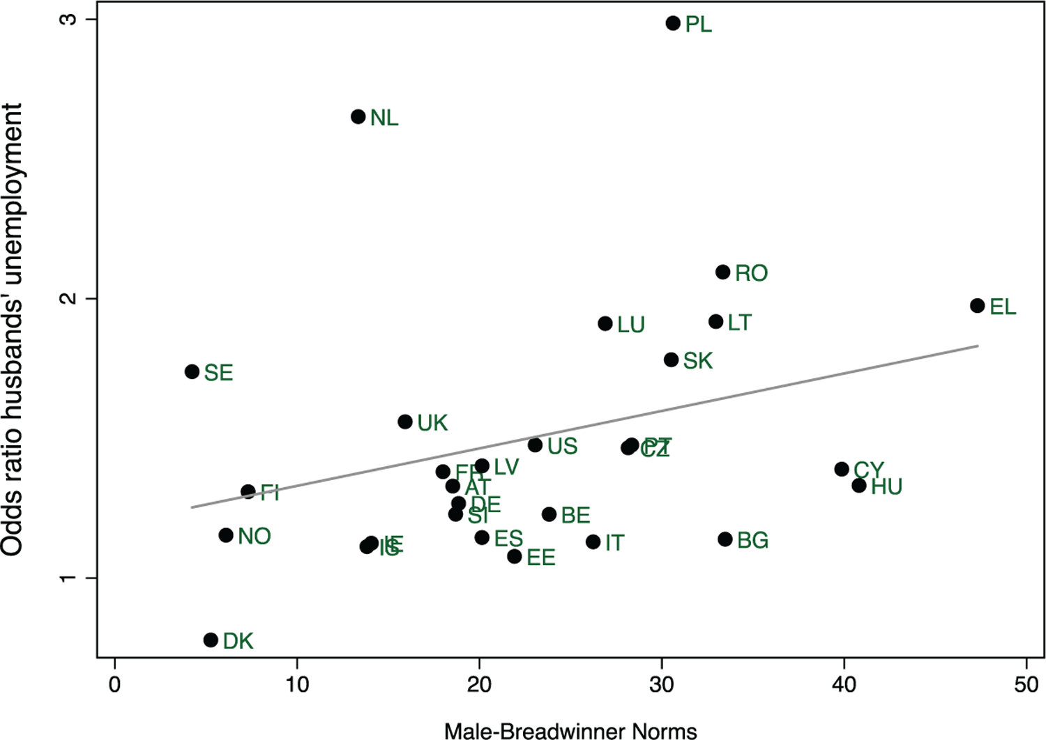
Divorce Odds Ratio for Men’s Unemployment by Male-Breadwinner Norms
Data sources: SIPP (US), GSOEP (DE), BHPS and UKHLS (UK), EU-SILC (all other countries).
Note: The figure plots coefficients from a pooled logistic regression with country fixed-effects interacted with men’s unemployment and individual-level control variables.
Country legend: AT = Austria, BE = Belgium, BG = Bulgaria, CY = Cyprus, CZ = Czech Republic, DE = Germany, DK = Denmark, EE = Estonia, EL = Greece, ES = Spain, FI = Finland, FR = France, HU = Hungary, IE = Ireland, IS = Iceland, IT = Italy, LT = Lithuania, LU = Luxembourg, LV = Latvia, NL = Netherlands, NO = Norway, PL = Poland, PT = Portugal, RO = Romania, SE = Sweden, SI = Slovenia, SK = Slovakia, UK = United Kingdom, US = United States.
Table 3 presents results for the first part of our analysis. We first discuss the baseline model (Model 1) and then test our hypotheses in subsequent models. Consistent with previous studies, we find that unemployment clearly increases the risk of separation. Model 1 estimates that, compared to couples who do not experience unemployment, couples in which either partner experienced unemployment are more likely to be separated in the following year. In line with prior work, the size of men’s unemployment coefficient is larger than women’s (Eliason 2012; Jalovaara 2003; Jensen and Smith 1990). Because the baseline model does not yet control for earnings, the larger size of men’s unemployment coefficient could be due to the fact that his earnings are typically higher than hers and that, consistent with the financial strain approach, his job loss puts the family under greater financial stress. The coefficients of control variables are as expected. Cohabiting couples have a much higher risk of dissolution than do married couples. Higher levels of education of either partner lower the risk of separation, as do both types of couple investments, having young children, and home ownership.
Table 3.
Three-Level Logistic Regression on the Annual Probability of Separation
| Variables | Model 1 | Model 2 | Model 3 | Model 4 | Model 5 | Model 6 |
|---|---|---|---|---|---|---|
| Women’s unemployment | .134*** (.034) |
.131*** (.035) |
.126*** (.035) |
.206*** (.037) |
.225*** (.038) |
.224*** (.038) |
| Men’s unemployment | .419*** (.046) |
.397*** (.032) |
.396*** (.033) |
.280*** (.059) |
.346*** (.037) |
.332*** (.036) |
| Male-breadwinner norms | .030** (.009) |
.033** (.010) |
.033** (.010) |
.033*** (.010) |
.033** (.010) |
|
| # W Unemp | .004 (.004) |
.005 (.004) |
.004 (.004) |
.004 (.004) |
.004 (.004) |
|
| # M Unemp | .011** (.004) |
.012** (.004) |
.012** (.004) |
.011** (.004) |
.012** (.004) |
|
| Family income (logged) | −.005 (.005) |
−.001 (.005) |
||||
| Men’s relative earnings | −.291*** (.047) |
|||||
| # M Unemp | .083 (.092) |
|||||
| Women’s earnings (logged) | .023*** (.004) |
.023*** (.004) |
||||
| Men’s earnings (logged) | −.020*** (.004) |
−.020*** (.004) |
||||
| Gender wage gap | .059*** (.015) |
|||||
| # M Unemp | −.009 (.006) |
|||||
| Women’s education | ||||||
| Secondary | .016 (.024) |
.018 (.024) |
.021 (.024) |
.011 (.025) |
.011 (.025) |
.011 (.025) |
| College | −.115** (.040) |
−.113** (.040) |
−.119** (.040) |
−.145*** (.040) |
−.138*** (.040) |
−.139*** (.040) |
| Men’s education | ||||||
| Secondary | .001 (.023) |
−.001 (.023) |
.006 (.024) |
.010 (.024) |
.008 (.024) |
.008 (.024) |
| College | −.214*** (.030) |
−.214*** (.030) |
−.207*** (.031) |
−.193*** (.031) |
−.200*** (.031) |
−.200*** (.031) |
| Cohabitation | 1.828*** (.135) |
1.801*** (.136) |
1.796*** (.137) |
1.790*** (.137) |
1.788*** (.137) |
1.789*** (.137) |
| Household tenure | −.395*** (.021) |
−.396*** (.021) |
−.399*** (.021) |
−.395*** (.021) |
−.398*** (.021) |
−.398*** (.021) |
| Constant | −1.350*** (.423) |
−1.418*** (.425) |
−1.380*** (.431) |
−1.248*** (.435) |
−1.433*** (.431) |
−1.437*** (.436) |
| Random intercepts | Yes | Yes | Yes | Yes | Yes | Yes |
| Random slopes | Yes | Yes | Yes | Yes | Yes | Yes |
| Observations | 978,200 | 978,200 | 978,200 | 978,200 | 978,200 | 978,200 |
| Number of groups | 290 | 290 | 290 | 290 | 290 | 290 |
Note: All models also control for women’s age (quadratic), parental status, women’s and men’s inactivity, and macro-level controls for GDP, UR, UGEN, GWG, and WLFP. Random intercepts at the country and country-year levels. Random slopes for men’s and women’s unemployment, college education, and cohabitation. Coefficients for the random components are omitted in the interest of space. Standard errors are clustered at the country and country-year levels.
p < .05
p < .01
p < .001 (two-tailed tests).
Model 2 presents a first test about our key mechanism of interest. We find that the cross-level interaction between men’s unemployment and male-breadwinner norms is statistically significant, but the interaction between women’s unemployment and male-breadwinner norms is not. These results indicate that when the male partner is unemployed, the risk of separation is higher in contexts with a high prevalence of male-breadwinner norms than in contexts with lower prevalence. This result is consistent with the gender social stress mechanism (Hypothesis 1). In countries with average male-breadwinner norms, the odds of separation are 49 percentage points higher among couples with unemployed male partners, exp(.397 + [0 × .011]) = 1.49.10 The odds ratio goes up to 65 percentage points with an increase of one standard deviation in the male-breadwinner norms scale, exp(.397 + [9.4 × .011]) = 1.65. We compute average marginal effects (AME) to evaluate the interaction and the magnitude of these patterns on the natural metric, the probability (Mize 2019).
Table 4 presents AMEs for selected models and reports Wald tests for group differences of interest. AMEs confirm that the interaction captures sizeable patterns. Panel B shows that an increase of one standard deviation in male-breadwinner norms increases men’s unemployment AME by .003, which represents a 60 percent increase from the overall men’s unemployment AME (.005). For reference, the baseline annual probability of divorce is estimated at .004 or .4 percent for this sample, the AME of home ownership is –.003, and the AME for children in the home is –.001. These calculations indicate that the magnitude of the gender social stress mechanism is comparable to, if not larger than, other well-known correlates of separation.
Table 4.
Men’s and Women’s Unemployment Average Marginal Effects (AME) and Wald Tests for Differences between Men’s and Women’s AMEs and for Differences between Men’s AMEs across Male-Breadwinner Norms and across Models
| Model 2 | Model 4 | Model 6 | Model 11 | ||
|---|---|---|---|---|---|
| A. AME | Men Women |
.005*** .001*** |
.004*** .002*** |
.004*** .002*** |
.004*** .002*** |
| Tests of Differences | |||||
| B. Men’s AME across BWN | Average – Low High – Average |
.002*** | .002*** | .002*** | .002*** |
| C. Women’s AME – Men’s AME | Overall | .003** −.004*** |
.003*** −.002** |
.003** −.002** |
.003** −.002** |
| D. Men’s AME across Models | Overall | baseline | .001 | .001 | .001 |
Data sources: SIPP (US), GSOEP (DE), BHPS and UKHLS (UK), EU-SILC (all other countries).
Note: Average marginal effects (AMEs) are computed based on regression models reported in Tables 3 and 5, that is, Model 2 AMEs correspond to Model 2 in Table 3. Panel A reports AMEs for men’s and women’s unemployment. The remainder of the panel reports two-sided Wald tests to determine whether differences between marginal effects are statistically significant within and across models. Panel B reports Wald tests for differences between the AME of men’s unemployment at different levels of male-breadwinner norms (BWN); average is the sample average for BWN, low is one standard deviation below it, and high is one standard deviation above it. Panel C reports Wald tests for differences between the AME of women’s and men’s unemployment. Panel D reports Wald tests for differences between men’s unemployment AMEs across models (here, Model 2 AMEs serve as the baseline category). In this last test we assume covariances between AMEs to be 0; this is a tentative test because appropriate tests for multilevel models have not yet been developed (Mize, Doan, and Long 2019).
p < .05
p < .01
p < .001 (two-tailed tests).
Although encouraging, results in Model 2 could be misleading if they were confounded by other well-known mechanisms that link men’s unemployment and separation, in particular the financial stress and economic specialization mechanisms. Models 3 to 6 present different operationalizations for these mechanisms to evaluate whether they confound the cross-level interaction and to assess their independent relevance to the risk of unemployment-related separation. Model 3 controls for financial stress via couples’ total income. In considering Hypothesis 2, we find little evidence that financial stress mediates the relationship between men’s unemployment and separation. The coefficient for family income is not statistically significant and the coefficient for men’s unemployment does not change much after controlling for financial stress.
Models 4 to 6 present distinct operationalizations to control for the economic specialization mechanism, and they confirm that the cross-level interaction finding remains robust. Model 4 tests whether the relationship between men’s unemployment and separation is moderated by men’s relative monthly earnings. The interaction coefficient is not statistically significant, showing no support for Hypothesis 3. Consistent with expectations of the general prediction of the economic specialization model (Hypothesis 3b), however, we do find that couples in which men out-earn their partners have lower risk of separation net of family income. Panel D in Table 4 shows that the difference between men’s unemployment AMEs in Models 2 and 4 are not statistically significant, providing little evidence of mediation. Model 5 enters separate control variables for his and her incomes as a synthetic flexible operationalization for both financial stress and gendered economic specialization mechanisms and shows that the interaction finding is also robust. This model shows that women’s earnings increase the risk of divorce and men’s earnings reduce it, a finding consistent with the general expectations of the economic specialization theory (Weiss and Willis 1997), but there is little evidence that these controls mediate the association between unemployment and separation (Hypothesis 3b). The Wald test in Panel D of Table 2 is again not statistically significant.
Model 6 presents the context-level operationalization of the economic specialization model, testing whether the relationship between men’s unemployment and separation is moderated by the context-level gender wage gap. The interaction between men’s unemployment and the context-level gender wage gap is not statistically significant, failing to support the hypothesis that context-level variation in men’s relative advantage in market productivity would moderate the association between men’s unemployment and separation (Hypothesis 3). Importantly, the cross-level interaction between men’s unemployment and male-breadwinner norms remains largely unchanged and robust across all models, indicating that support for the gender social stress interpretation remains robust. Panel B in Table 4 shows that differences between men’s unemployment AMEs across levels of male-breadwinner norms are statistically significant and similar across all models.
The results thus far offer substantial evidence in favor of the gender social stress mechanism, showing that men’s unemployment is more strongly associated with divorce in contexts where male-breadwinner norms are prevalent even after controlling for financial stress and economic specialization mechanisms. Figure 2 illustrates this finding by plotting the marginal effects of men’s and women’s unemployment across different levels of male-breadwinner norms. As the proportion of the population that supports the male-breadwinner model increases, the marginal effect for men’s unemployment also grows. In countries with below-average support for male-breadwinner norms (support below 22 percent), the marginal effect of men’s unemployment is low and close to the marginal effect for women’s unemployment. In countries with above-average male-breadwinner norms, the marginal effect of men’s unemployment is much higher, and the marginal effect for women’s unemployment remains lower.
Figure 2.
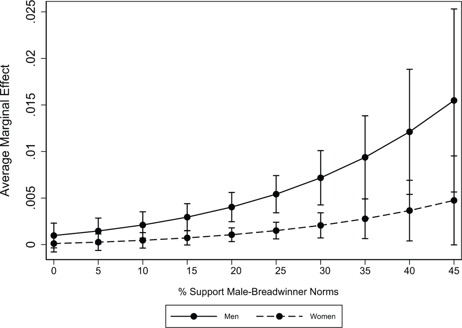
Men’s and Women’s Unemployment Average Marginal Effects by Male-Breadwinner Norms
Data sources: SIPP (US), GSOEP (DE), BHPS and UKHLS (UK), EU-SILC (all other countries).
Although Models 3 to 6 include key micro-and macro-level control variables, it is possible for the cross-level interaction between men’s unemployment and male-breadwinner norms to be spurious if male-breadwinner norms correlate with other context-level processes that lead to higher separation risks among unemployed men. Table 5 presents analyses to check the robustness of this finding to additional cross-level interactions. Models 7 to 10 test for cross-level interactions with other macro-level economic variables one by one; gross domestic product (GDP), unemployment rate (UR), unemployment benefit generosity index (UGEN), and women’s employment rate (WLFP). Model 11 includes all cross-level interactions. These analyses confirm that support for Hypothesis 1 remains robust and show that all other cross-level interactions, with the exception of the interaction between men’s unemployment and unemployment benefit generosity, are not statistically significant. The main effects for context-level control variables are mostly not statistically significant, except for positive and statistically significant coefficients for gender wage gap, unemployment benefit generosity, and unemployment rate in some models. Table S6 in the online supplement presents additional robustness checks for context-level unobserved heterogeneity, in particular models that use country fixed-effects, year fixed-effects, and country fixed-effects interacted with men’s unemployment (also called FEs models in Giesselmann and Schmidt-Catran 2019). Our finding that men’s unemployment is moderated by context-level male-breadwinner norms remains robust through all these stringent tests. Taken together, our key finding supporting the gender social stress mechanism, that strongly held male-breadwinner norms correlate with an increased association between men’s unemployment and separation risk, is robust to an extensive set of potential confounders.
Table 5.
Three-Level Logistic Regression on the Annual Probability of Separation, Context-Level Robustness Checks
| Variables | Model 7 Interaction with GDP | Model 8 Interaction with UR | Model 9 Interaction with UGEN | Model 10 Interaction with WLFP | Model 11 Interaction with All Macro Variables |
|---|---|---|---|---|---|
| Women’s unemployment | .224*** | .224*** | .214*** | .224*** | .225*** |
| (.038) | (.038) | (.040) | (.038) | (.038) | |
| Men’s unemployment | .332*** | .338*** | .338*** | .333*** | .355*** |
| (.036) | (.036) | (.038) | (.036) | (.038) | |
| Male-breadwinner norms | .033*** | .033*** | .042*** | .033** | .033*** |
| (.010) | (.010) | (.011) | (.010) | (.010) | |
| # W Unemp | .004 | .004 | .005 | .004 | .004 |
| (.004) | (.004) | (.005) | (.004) | (.004) | |
| # M Unemp . | 011** | .012** | .011** | .012** | .011** |
| (.004) | (.004) | (.004) | (.004) | (.004) | |
| Women’s earnings (logged) | .023*** | .023*** | .021*** | .023*** | .023*** |
| (.004) | (.004) | (.004) | (.004) | (.004) | |
| Men’s earnings (logged) | −.020*** | −.020*** | −.018*** | −.020*** | −.020*** |
| (.004) | (.004) | (.004) | (.004) | (.004) | |
| GDP | −.006 | −.005 | −.016** | −.005 | −.006 |
| (.005) | (.005) | (.006) | (.005) | (.005) | |
| # M Unemp | .001 | .001 | |||
| (.002) | (.002) | ||||
| UR | .057* | .060* | .097** | .057* | .060* |
| (.027) | (.027) | (.037) | (.027) | (.027) | |
| # M Unemp | −.015 | −.015 | |||
| (.015) | (.016) | ||||
| UGEN | .010* | .010* | .007 | .010* | .010* |
| (.004) | (.004) | (.004) | (.004) | (.004) | |
| # M Unemp | .005** | .003 | |||
| (.002) | (.002) | ||||
| WLFP | −.945 | −.946 | −.074 | −.962 | −.965 |
| (1.021) | (1.021) | (1.043) | (1.023) | (1.023) | |
| # M Unemp | .124 | .186 | |||
| (.473) | (.493) | ||||
| GWG | .058*** | .058*** | .062*** | .058*** | .059*** |
| (.015) | (.015) | (.015) | (.015) | (.015) | |
| # M Unemp | −.009 | ||||
| (.006) | |||||
| Constant | −1.431*** | −1.437*** | −1.301** | −1.434*** | −1.440*** |
| (.431) | (.431) | (.446) | (.431) | (.431) | |
| Random intercepts | Yes | Yes | Yes | Yes | Yes |
| Random slopes | Yes | Yes | Yes | Yes | Yes |
| Observations | 978,200 | 978,200 | 978,200 | 978,200 | 978,200 |
| Number of groups | 290 | 290 | 290 | 290 | 290 |
Note: Models also control for women’s age (quadratic), parental status, women’s and men’s inactivity and education levels, and household tenure. Random intercepts at the country and country-year levels. Random slopes for men’s and women’s unemployment, college education, and cohabitation. Coefficients for the random components are omitted in the interest of space. Standard errors are clustered at the country and country-year levels.
p < .05
p < .01
p < .001 (two-tailed tests).
Having established the substantial moderating effect of context-level male-breadwinner norms on separation risk, we move to test subsequent hypotheses about functional form (Hypothesis 1a). Existing theoretical developments about the gender social stress mechanism typically do not specify a functional form, but some work suggests there might be a curvilinear relationship between context-level norms and behavior (Breen and Cooke 2005; Esping-Andersen and Billari 2015). Table 6, Model 12, adds a quadratic term to allow male-breadwinner norms to moderate the association between men’s unemployment and separation in a nonlinear fashion. The results show evidence in support of the curvilinear specification, albeit modest; the interaction with the quadratic term is statistically significant and the log-likelihood ratio test indicates model improvement (LR chi2(2) = 12.79; p = .002). Figure 3 provides a visual representation of this result. Because the logistic model already implicates a nonlinear interaction on the probability metric, the plotted shape of men’s unemployment AME does not dramatically change, but it changes in a direction consistent with the idea of a tipping point (Breen and Cooke 2005). We find that the association between men’s unemployment and the risk of separation is relatively flat when the prevalence of male-breadwinning values ranges between 0 and 15 percent, and it only starts increasing when the prevalence of male-breadwinning norms hits 20 percent. Supplementary tests also show that small increases in male-breadwinner norms are only statistically significant when the overall support for male-breadwinner norms is above 15 to 20 percent (see Part C of the online supplement). Further research is needed to examine this hypothesis in more depth, but our results are generally consistent with the threshold model.
Table 6.
Three-Level Logistic Regression on the Annual Probability of Separation, Additional Models
| Variables | Model 12 Quadratic | Model 13 Interaction w/Cohabitation | Model 14 Married Couples | Model 15 Cohabiting Couples |
|---|---|---|---|---|
| Women’s unemployment | .225*** | .225*** | .286*** | .159** |
| (.038) | (.038) | (.059) | (.051) | |
| Men’s unemployment | .297*** | .388*** | .325*** | .308*** |
| (.041) | (.052) | (.064) | (.047) | |
| Cohabiting | 1.788*** | 1.802*** | ||
| (.137) | (.144) | |||
| Male-breadwinner norms (BWN) | .035*** | .024* | .024** | .034*** |
| (.010) | (.010) | (.009) | (.009) | |
| # W Unemp | .004 | .004 | .004 | .001 |
| (.004) | (.004) | (.006) | (.006) | |
| # M Unemp | .010** | .017** | .019** | −.002 |
| (.003) | (.006) | (.006) | (.005) | |
| # BWN^2 | .001* | |||
| (.000) | ||||
| # BWN^2 # M Unemp | −.001* | |||
| # Cohabiting | (.000) | .027*** | ||
| (.006) | ||||
| # Cohabiting # M Unemp | −.013* | |||
| (.005) | ||||
| Women’s education | ||||
| Secondary | .011 | .011 | .023 | −.003 |
| (.025) | (.025) | (.036) | (.034) | |
| College | −.137*** | −.139*** | −.110 | −.177*** |
| (.040) | (.040) | (.061) | (.052) | |
| Men’s education | ||||
| Secondary | .008 | .006 | .047 | −.033 |
| (.024) | (.024) | (.035) | (.032) | |
| College | −.200*** | −.201*** | −.260*** | −.129** |
| (.031) | (.031) | (.044) | (.043) | |
| Household tenure | −.398*** | −.397*** | −.513*** | −.301*** |
| (.021) | (.021) | (.031) | (.029) | |
| Constant | −1.287** | −1.440*** | −4.624*** | 1.904*** |
| (.436) | (.430) | (.859) | (.520) | |
| Random intercepts | Yes | Yes | Yes | Yes |
| Random slopes | Yes | Yes | Yes | Yes |
| Observations | 978,200 | 978,200 | 782,560 | 195,640 |
| Number of groups | 290 | 290 | 282 | 282 |
Note: Models also control for women’s age (quadratic); parental status; women’s and men’s inactivity, educational levels, and incomes (logged); household tenure; and GDP, UR, UGEN, GWG, and WLFP. Random intercepts at the country and country-year levels. Random slopes for men’s and women’s unemployment, college education, and cohabitation. Coefficients for the random components are omitted in the interest of space. Standard errors are clustered at the country and country-year levels.
p < .05
p < .01
p < .001 (two-tailed tests).
Figure 3.
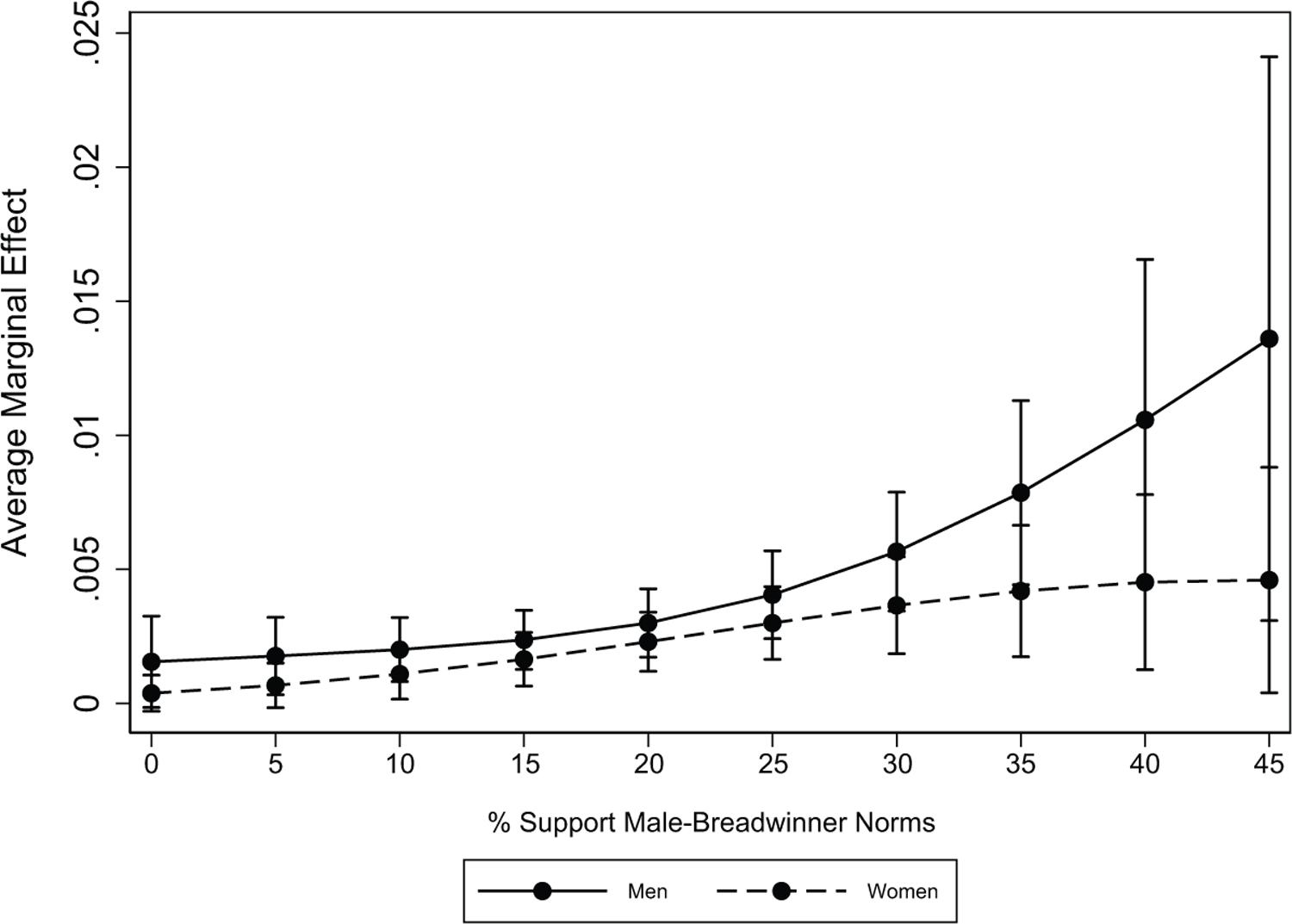
Men’s and Women’s Unemployment Average Marginal Effects by Male-Breadwinner Norms, Quadratic Specification
Data sources: SIPP (US), GSOEP (DE), BHPS and UKHLS (UK), EU-SILC (all other countries).
Finally, we examine the proposition that male-breadwinner norms apply more strongly to married than to cohabiting couples (Hypothesis 1b). Both gender and social institutionalist theorists propose reasons to expect conforming to gender expectations is more consequential for married unions than for cohabiting unions (Brines and Joyner 1999). Model 13 in Table 6 adds a three-way interaction between men’s unemployment, male-breadwinner norms, and a cohabitation dummy. The results indicate that the relevance of context-level gender norms varies by union type. This result suggests married men’s unemployment coefficient is more sensitive to changes in male-breadwinner norms than is cohabiting men’s unemployment coefficient. Models 14 and 15 report separate regressions by marital status that replicate the same pattern. They show the interaction with male-breadwinner norms is only statistically significant for married couples, not for cohabiting couples.
Figure 4 and Table 7 present AMEs to evaluate these results on the probability scale. Unlike the logistic coefficients, AME patterns suggest the cohabiting men’s unemployment coefficient also varies across male-breadwinner norms, but this variation is relatively smaller and not statistically significant as that among married couples.11 Detailed tests about these patterns of variation among married and cohabiting couples confirm this reading (see Figure S5 in the online supplement). It is possible that the lack of statistically significant variation in cohabiting men’s unemployment AMEs across male-breadwinner norms could be due to statistical power issues in the smaller cohabiting sample. Although we cannot rule this out, the differences in slopes between these two types of unions are notable and thus point to a substantive difference. Taken together, these results support Hypothesis 1b and are consistent with the view that deviating from the conventional division of labor is more disruptive for marriages than for cohabiting couples. These analyses cannot directly answer whether the difference between married and cohabiting couples is produced by differences in the institutionalization of incentives for the conventional division of labor (Brines and Joyner 1999) or by differences in the social expectations that couples are beholden to (Shelton and John 1993). Further research is needed to disentangle these mechanisms.
Figure 4.
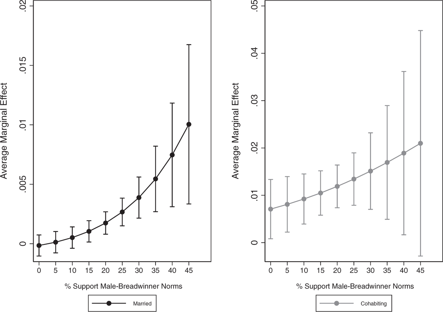
Average Marginal Effect of Men’s Unemployment in Married and Cohabiting Unions by Male-Breadwinner Norms
Data sources: SIPP (US), GSOEP (DE), BHPS and UKHLS (UK), EU-SILC (all other countries).
Table 7.
Men’s and Women’s Unemployment Average Marginal Effects (AME) and Wald Tests for Differences between Men’s and Women’s AMEs and for Differences between Men’s AMEs across Male-Breadwinner Norms
| Model 12 |
Model 13 |
|||
|---|---|---|---|---|
| Quadratic | Married | Cohabiting | ||
| A. AME | Men | .004*** | .003*** | .010*** |
| Women | .002*** | .001*** | .008*** | |
| Tests of Differences | ||||
| B. Men’s AME across BWV | Average – Low | .001** | .001*** | .004** |
| High – Average | .003*** | .003** | .007* | |
| C. Men’s AME – Women’s AME | Overall | −.002** | −.001*** | −.002 |
Data sources: SIPP (US), GSOEP (DE), BHPS and UKHLS (UK), EU-SILC (all other countries). Note: Average marginal effects (AMEs) are computed based on regression models reported in Table 6, that is, Model 13 AMEs correspond to Model 13 in Table 6. Panel A reports AMEs for men’s and women’s unemployment. The remainder of the panel reports two-sided Wald tests to determine whether differences between marginal effects across groups are statistically significant. Panel B reports Wald tests for differences between the AME of men’s unemployment at different levels of male-breadwinner norms (BWN); average is the sample mean for BWN, low is one standard deviation below the mean, and high is one standard deviation above the mean. Panel C reports Wald tests for differences between the AME of women’s and men’s unemployment.
p < .05
p < .01
p < .001 (two-tailed tests).
Other Robustness Checks
We conducted a number of additional robustness checks to address limitations in measurement and omitted variable bias. One weakness of the analysis is the measure of unemployment, which does not distinguish between job loss and other forms of unemployment, such as looking for jobs after finishing school or after a period of economic inactivity. This is problematic because unemployment not related to job loss might be less prone to raise relationship conflicts, as suggested by research that disaggregates different types of unemployment and sources of job loss (e.g., layoffs versus plant closure) (Charles and Stephens 2004; Doiron and Medolia 2011; Eliason 2012). We conducted sensitivity analyses using a subset of countries for which we have employment calendar information where unemployment solely indicates actual job loss. We used the previous year’s employment calendar to code transitions from employment to unemployment, including left-censored cases (or individuals who are observed unemployed at the beginning of the employment calendar). Because we do not know the origin of left-censored unemployment spells, we include a control variable for labor force attachment to capture cases of unemployment among individuals who have weak attachment to the labor market. Table S5 in the online supplement reports results and shows that patterns discussed above are replicated with this restricted sample. This confirms that our findings reflect job losses and are not a product of other forms of unemployment.
A separate concern pertains to the question of whether our estimate for men’s unemployment can be considered a reasonable estimate of the causal effect of unemployment on separation, an assumption we make indirectly. Researchers have raised the possibility that unobserved heterogeneity and reverse causality processes can bias estimates of the association between men’s unemployment and separation—that is, unobserved individual attributes, like low commitment or laziness, can lead to both unemployment and separation, or relationship trouble can generate low worker productivity and lead to job loss and later separation (Covizzi 2008). Our data pose unfortunate limitations to implement robustness checks to explore this question. The two prominent correction methods (Mundlak correction and conditional logit models) require a substantial number of repeated observations to work well, and our data only include four repeated observations. Despite the inadequacy of our data, we applied these tests in an effort to address this concern. The results show the cross-level interaction remains robust to both types of corrections for unobserved heterogeneity at the individual level, confirming the robustness of our interpretation about the moderating role of context-level male-breadwinner norms.12 See Table S6 in the online supplement.
We conducted supplementary analyses to check the sensitivity of our results to additional specifications. Because our data cover the Great Recession, one concern might be that we are insufficiently able to capture both time-fixed and time-varying unobserved processes that might shape the meaning of unemployment.13 To assess concerns about context-level unobserved heterogeneity, Table S6 in the online supplement shows our results are robust to country fixed-effects, to the exclusion of recession years from our data (2009 to 2010), and to the exclusion of outliers identified in Figure 1. Our results might still be challenged by other time-varying context-level processes unrelated to the time-varying context-level variables included in the models. Table S4 in the online supplement shows our results are replicated using different operationalizations of the male-bread-winner norms measure and when we include interactions with other dimensions of gender norms, such as the level of agreement with the statement that children suffer when mothers work. Table S7 in the online supplement shows our results are also robust to additional interactions between men’s unemployment and individual-level covariates, in particular his age and his education. All these analyses show our main findings and patterns are robust to numerous alternative specifications.
DISCUSSION
This study offers a novel test of the idea that gender culture moderates the relationship between couples’ economic characteristics and union dissolution by measuring and leveraging variation in the key explanatory variable, context-level gender norms. We find that men’s unemployment is associated with higher risk of couple separation in countries where the male-breadwinner model is strongly embedded in social and cultural values, that is, where a substantial share of the population believes breadwinning is men’s primary role. In countries where only a small minority of the population believe breadwinning is men’s primary role, men’s unemployment is not as strongly linked to separation. Our findings are consistent with prior work emphasizing the importance of gender norms to understand stability in marriage (Cooke 2006; Killewald 2016; Sayer et al. 2011; Schwartz and Gonalons-Pons 2016; Schwartz and Han 2014). Prior studies have identified the gender stress mechanism without measuring gender norms, but our study measures the prevalence of support for the male-breadwinner model in different countries and correlates that data directly with the likelihood that men’s unemployment will increase the risk of separation. In this way, our study provides a new, robust test of the gender social stress mechanism.
The results indicate that union type matters, too. We find that male-breadwinner norms moderate the association between men’s unemployment and separation more strongly among married couples than among cohabiting couples. This pattern is consistent with gender theorists’ suggestion that gender norms are context-specific and that marriage heightens gender expectations (Risman 1999). It is also consistent with work suggesting that institutions set stronger incentives for the gendered division of labor for married couples than for cohabiting couples (Brines and Joyner 1999). Because our results are robust to stringent controls for fixed context-level heterogeneity, and our sample includes a variety of countries with different levels of institutionalized benefits for married couples, we see our findings as more consistent with the gender social expectation mechanism than with the institutional mechanism. However, future research is needed to further disentangle these two mechanisms.
Our analyses also offer evidence consistent with some tenets of the financial strain and economic specialization approaches, but the evidence that these mechanisms moderate the relationship between unemployment and separation is more limited. We find evidence that men’s higher income is associated with lower risk of separation, but we do not find that controlling for financial strain mediates the relationship between his unemployment and separation. This is contrary to results in previous studies finding that economic stress mediates the association between unemployment and separation (Blekesaune 2009; Hansen 2005; Poortman 2005), but consistent with studies that do not find support for such mediation (Charles and Stephens 2004; Doiron and Medolia 2011). Similarly, we find evidence that men’s relative market advantage is associated with a lower risk of separation, but we find no evidence that his relative market advantage moderates (or mediates) the association between his unemployment and separation.
Our study is not without shortcomings. The rotating panel structure limits our ability to construct more precise measures for long-term income patterns. There is missing information on union parity and duration, and we cannot entirely rule out omitted variable bias (but in the online supplement, see Table S7 for sensitivity tests and Part D for a detailed evaluation of this concern). Similarly, couple-level measures about relationship satisfaction and gender attitudes would offer additional venues to test these theoretical approaches and address potential confounders. The lack of information on couples’ gender attitudes is particularly significant. Our data cannot entirely separate the extent to which the gender norm mechanism is working as a genuine contextual process that influences all couples irrespective of gender ideology, and the extent to which it is working through couples’ gender attitudes (i.e., if it manifests only in couples with male-breadwinner preferences). The robustness of our findings to controlling for education and age that correlate with gender attitudes, as well as controlling for the interaction between men’s unemployment and these two variables,14 boosts our confidence that the findings point to a contextual-level process, but future analyses combining data on context-level norms and couple-level attitudes could address this issue more directly. Finally, the measure of the male-breadwinner norm is imperfect for two main reasons: it combines items from two different surveys and it only includes data from two points in time, which might not capture subtler changes in gender norms over time (Knight and Brinton 2017). Although we thoroughly tested alternative specifications (see Table S4 in the online supplement), we cannot entirely rule out measurement error. Future analyses could also leverage regional variation within countries with better measures on gender norms to address these issues.
Our findings have implications for discussions about changes in gender norms, in particular, changes in gender norms about masculinity. In light of the gender revolution, attitudes toward women’s economic roles have shifted much faster and further than attitudes toward men’s economic roles (England 2010). This has led some scholars to suggest the change in gender culture is multidimensional, and new modes of gender egalitarianism might emerge without challenging the male-breadwinner norm (Dernberger and Pepin 2020; Knight and Brinton 2017; Pepin and Cotter 2018). By broadening the range of gender cultures, our study includes contexts where the support for the male-breadwinner norm is low, and our results indicate that the gender social stress mechanism does notably decline as a result. We find that in countries with below-average support for male-breadwinner norms, men’s unemployment is much less likely to result in separation, ceteris paribus. Thus, although the male-breadwinner norm might remain strong in certain contexts, in other contexts it does not, and this increases couples’ relationship stability when the male partner experiences unemployment.
These results suggest that cultural changes challenging male-breadwinner culture can have real benefits for romantic relationships. Our theoretical framework argues these benefits are due to the removal of pressures to fulfill gendered expectations. This process is consistent with research documenting the lived experience of these pressures—that is, studies demonstrating that family and friends show greater disappointment and disapproval of men’s job loss than women’s job loss (Jahoda et al. 1933; Rijken and Liefbroer 2016), that men suffer more emotionally from job loss than do women (Cooper 2014; Rao 2020), and that couples feel a more intense need to account for men’s job loss than for women’s (Rao 2020; Tichenor 2005). By systematically analyzing cross-cultural variation, we have offered novel quantitative evidence about the relevance of gender culture in shaping societal understandings of unemployment and romantic relationships and in framing how individuals feel about and respond to job loss.
Supplementary Material
Acknowledgments
We thank the ASR editors and reviewers for their feedback and constructive guidance throughout the review process. We are also grateful to Kristina Lindemann, Carlotta Giustozzi, Jan Brülle, Timo Lepper, Rona Geffen, Anne Kronberg, Fabian Ochsenfeld, David Calnitsky, Kelly Musick, Christine Schwartz, and Paul D. Allison for comments and suggestions on earlier drafts.
Funding
This research has been supported by the European Research Council under the European Union’s Seventh Framework Programme (FP7/2007-2013, ERC grant agreement n° ERC-2013-CoG-615246-CORRODE).
Biography
Pilar Gonalons-Pons is an Assistant Professor of Sociology at the University of Pennsylvania. Her research examines how work, gender, families, and public policies structure economic inequalities. She has published on economic homogamy and income inequality, on the transition to parenthood and economic inequalities within and between families, and on housework outsourcing and the gender division of household labor. In current projects she examines how the social organization of care and reproductive paid and unpaid work shapes economic inequalities.
Markus Gangl is a Professor of Sociology at the Department of Social Sciences at the Goethe-University in Frankfurt am Main and an Honorary Fellow at the Department of Sociology at the University of Wisconsin-Madison. He works on issues of social stratification, economic inequality, poverty, income dynamics, social mobility, labor markets, and careers. He is the principal investigator of two ERC-funded projects to examine the socioeconomic repercussions of the Great Recession and increasing economic inequality in Europe and North America, and he currently serves as the Editor-in-Chief of the European Sociological Review.
Footnotes
Evidence about gender compensatory behavior is found in many realms of social life (for recent quantitative studies finding support for gender compensatory behaviors in infidelity, housework, health, and attitudes, see Munsch 2015; Schneider 2012; Springer 2010; Willer et al. 2013). The evidence about gender compensatory behavior applied to the relationship between relative earnings and housework is, however, contested, particularly in studies analyzing data from the United States. A first wave of research on this topic found evidence for the gender compensatory behavior on the relationship between relative earnings and housework, supporting the hypothesis that women do more housework when they earn more than their male partners or that men do less (Bittman et al. 2003; Brines 1994; Greenstein 2000). A second wave of research disputed these findings (Gupta 1999, 2006, 2007; Gupta and Ash 2008; Killewald and Gough 2010). Since then, some studies using U.S. data have found support for this hypothesis (Schneider 2011; Vijayasiri 2011) and others have not (Hook 2017). Recent non-U.S. studies have found evidence for compensatory behavior in the relationship between relative earnings and housework in Germany (Procher, Ritter, and Vance 2018); in Belgium, France, Romania, and Russia (Aassve, Fuochi, and Mencarini 2014); and in gender conservative countries using the International Social Survey Program cross-national dataset (Mandel et al. 2020).
An adjacent body of literature studies the relationship between context-level unemployment, or macroeconomic conditions, and divorce, instead of couple-level unemployment experiences. Some of these studies find evidence that higher unemployment rates and economic recessions are associated with lower divorce rates (Amato and Beattie 2011; Cherlin et al. 2013; Chowdhury 2013; González-Val and Marcén 2017; Hellerstein and Morrill 2011; Kalmijn 2007; Schaller 2013) and lower likelihood of divorce (Hellerstein, Morrill, and Zou 2013). These studies support the “costs of divorce” approach, which poses that economic insecurity and uncertainty reduce the likelihood of separation because it makes couples depend more on each other. Other studies, however, question these results and note that estimated declines may likely be delays in divorce (Cohen 2014; Lyngstad 2011; South 1985; Stevenson and Wolfers 2007). Findings concerning context-level unemployment are mixed, but findings concerning men’s unemployment are largely consistent in indicating its association with higher divorce risks. Our analyses include controls for the context-level unemployment rate, but we will not discuss this variable in detail because the focus of our study is on the cultural and economic mechanisms of individual-level economic correlates of separation.
The magnitude of the decline in relative utility gains of remaining in the relationship also depends on how much of it is offset by utility gains from home production. Households also might gain utility from more home production of its adult members. In fact, classic models, which assumed economic specialization as the utility maximizing strategy, expected women’s unemployment to be advantageous because it contributed to home production. Even if households could gain home production from men’s unemployment, the prediction is that the loss in market production would be larger and thus result in a net decline in utility.
Operationalizations of the economic specialization mechanism depend on assumptions about what maximizes utility, which can vary across couples and contexts. We choose a flexible operationalization that connects utility gains to earnings potential; this assumes couples derive greater utility gains (losses) from earnings gains (losses) of the member of the couple with the higher earnings potential. This operationalization is more flexible than the conventional assumption that full economic specialization (breadwinning–homemaking) maximizes utility for all couples. All substantive results are robust to alternative operationalizations.
Like other studies with similar data, one limitation of this measure is that it does not capture earnings losses incurred if unemployment starts the year of the interview. We conducted sensitivity checks to evaluate the extent to which this measurement limitation could underestimate financial strain induced by unemployment. We confirmed that this issue affects only a small share of those who report being unemployed at the time of the survey, and that our results are robust to including an indicator variable for those who started unemployment in the survey year.
An alternative way to measure couple-level differentials in market productivities would be to calculate permanent income. Unfortunately, because our data only include four observations per couple, we cannot calculate this alternative measure. We also constructed tests with predicted earnings measures, but the occupational categories are too broad and the results are not informative.
We estimate a multilevel model for the annual probability of separation (i.e., between any two consecutive annual panel interviews) conditional on being in a union at the point of the baseline interview in the pair. Because we do not have information on union duration, our data structure corresponds to what is known in event history literature as “left-truncation with unknown start dates” (Guo 1993:219ff.), and our empirical model is an analog to a discrete-time event model that is restricted to assuming a time-constant baseline hazard absent empirical information on union start dates in the EU-SILC surveys (see Allison 1982; Guo 1993). In the online supplement, see Part D for a detailed evaluation of this issue and Table S7 for sensitivity tests.
Random slopes allow for country-level variation in key individual covariates and make sure estimated fixed coefficients are not driven by a combination of different compositions and effects across countries (Heisig and Schaeffer 2019). For instance, if the effect of unemployment on separation among cohabitating couples is smaller in countries where cohabitation is more common (Liefbroer and Dourleijn 2006), we would overestimate the fixed coefficient for cohabitation if many of our observations came from countries where cohabitation is rare. We also know that the educational gradient of separation varies across countries (Kalmijn 2013), and random slopes guarantee this variation does not bias the coefficients of interest. To keep the model setup reasonably parsimonious and computationally feasible, our preferred specification includes the random slopes for all variables involved in a cross-level interaction as well as random slopes for covariates where previous studies have established an association with relationship outcomes that varies across countries, namely cohabitation and women’s education. We conducted further robustness checks by estimating alternative models that include an expanded set of random slope parameters; our results are essentially unaffected. With the present data, the only random slope parameter to attain substantive relevance and to signal statistically significant residual variation at the context level is the random slope for cohabitation. Our results are also robust to modifications in the structure of the model, for instance, including random slopes at the country (level 3) and country-year (level 2) levels. For more details, see the section “Sensitivity to the Structure of the Model” and Table S8, Models S24 to S27, in the online supplement.
This model can also be written in hierarchical form:
The male-breadwinner norms variable is mean-centered in the model, thus 0 represents the sample average.
Panel B in Table 7 shows that married men’s unemployment AME doubles when male-breadwinner norms increase from average to high (men’s average AME is .003, and an increase in male-breadwinner norms from average to high increases men’s AME by .003 points), whereas cohabiting men’s unemployment AME increases by 70 percent when male-breadwinner norms increase from average to high.
The main effect for men’s unemployment is not statistically significant in these models, which we believe is not surprising because four observations per individual is not sufficient to separate the stable individual effect from the event of unemployment. We applied the Mundlak correction method to the German and UK data, for which we have more repeated observations, and the results show the association between men’s unemployment and separation remains robust after controlling for fixed unobserved individual-level heterogeneity. These supplementary results, together with the record of published research finding robust causal evidence for the relationship between men’s unemployment and divorce using model specifications that tackle concerns about endogeneity and reverse causality more directly than we can (Charles and Stephens 2004; Doiron and Medolia 2011), validate the underlying causal assumption we make in this study.
A body of research has considered the hypothesis that higher levels of unemployment might lower unemployment stigma and the negative effect of unemployment on individual outcomes (i.e., health or well-being), but the existing evidence consistent with this hypothesis is weak (see Oesch and Lipps 2013).
See Part B, Table S7, Models S22 and S23, in the online supplement.
References
- Aassve Arnstein, Fuochi Giulia, and Mencarini Letizia. 2014. “Desperate Housework: Relative Resources, Time Availability, Economic Dependency, and Gender Ideology across Europe.” Journal of Family Issues 35(8):1000–22 ( 10.1177/0192513X14522248). [DOI] [Google Scholar]
- Allison Paul D. 1982. “Discrete-Time Methods for the Analysis of Event Histories.” Sociological Methodology 13:61–98 ( 10.2307/270718). [DOI] [Google Scholar]
- Amato Paul R. 2010. “Research on Divorce: Continuing Trends and New Developments.” Journal of Marriage and Family 72(3):650–66 ( 10.1111/j.1741-3737.2010.00723.x). [DOI] [Google Scholar]
- Amato Paul R., and Beattie Brett. 2011. “Does the Unemployment Rate Affect the Divorce Rate? An Analysis of State Data 1960–2005.” Social Science Research 40:705–715 ( 10.1016/j.ssresearch.2010.12.012). [DOI] [Google Scholar]
- Basbug Gokce, and Sharone Ofer. 2017. “The Emotional Toll of Long-Term Unemployment: Examining the Interaction Effects of Gender and Marital Status.” RSF: The Russell Sage Foundation Journal of the Social Sciences 3(3):222–44 ( 10.7758/rsf.2017.3.3.10). [DOI] [Google Scholar]
- Baxter Janeen. 2005. “To Marry or Not to Marry: Marital Status and the Household Division of Labor.” Journal of Family Issues 26(3):300–321 ( 10.1177/0192513X04270473). [DOI] [Google Scholar]
- Becker Gary S. 1974. “A Theory of Marriage.” Pp. 299–351 in Economics of the Family: Marriage, Children, and Human Capital, edited by Schultz TW Chicago: University of Chicago Press and NBER. [Google Scholar]
- Becker Gary S., Landes Elisabeth M., and Michael Robert T. 1977. “An Economic Analysis of Marital Instability.” The Journal of Political Economy 85(6):1141–87 ( 10.1086/260631). [DOI] [Google Scholar]
- Berk Sarah F. 1985. The Gender Factory: The Apportionment of Work in American Households Berlin: Springer Science and Business Media. [Google Scholar]
- Bernard Jessie. 1982. The Future of Marriage New Haven, CT: Yale University Press. [Google Scholar]
- Bertrand Marianne, Kamenica Emir, and Pan Jessica. 2015. “Gender Identity and Relative Income within Households.” The Quarterly Journal of Economics 130(2):571–614 ( 10.1093/qje/qjv001). [DOI] [Google Scholar]
- Bittman Michael, England Paula, Sayer Liana C., Folbre Nancy, and Matheson George. 2003. “When Does Gender Trump Money? Bargaining and Time in Household Work.” American Journal of Sociology 109(1):186–214 ( 10.1086/378341). [DOI] [Google Scholar]
- Blekesaune Morten. 2009. “Unemployment and Partnership Dissolution.” Pp. 202–216 in Changing Relationships, edited by Brynin M and Ermisch J New York: Routledge. [Google Scholar]
- Bloome Deirdre, Burk Derek, and Leslie McCall. 2019. “Economic Self-Reliance and Gender Inequality between U.S. Men and Women, 1970–2010.” American Journal of Sociology 124(5):1413–67 ( 10.1086/702278). [DOI] [Google Scholar]
- Boeckmann Irene, Misra Joya, and Budig Michelle J. 2015. “Cultural and Institutional Factors Shaping Mother’s Employment and Working Hours in Postindustrial Countries.” Social Forces 93(4):1301–33 ( 10.1093/sf/sou119). [DOI] [Google Scholar]
- Breen Richard, and Cooke Lynn P. 2005. “The Persistence of the Gendered Division of Domestic Labour.” European Sociological Review 21(1):43–57 ( 10.1093/esr/jci003). [DOI] [Google Scholar]
- Brines Julie. 1994. “Economic Dependency, Gender, and the Division of Labor at Home.” American Journal of Sociology 100(3):652–88 ( 10.1086/230577). [DOI] [Google Scholar]
- Brines Julie, and Joyner Kara. 1999. “The Ties That Bind: Principles of Cohesion in Cohabitation and Marriage.” American Journal of Sociology 64(3):333–55 ( 10.2307/2657490). [DOI] [Google Scholar]
- Bryan Mark L., and Jenkins Stephen P. 2016. “Multilevel Modelling of Country Effects: A Cautionary Tale.” European Sociological Review 32(1):3–22. [Google Scholar]
- Charles Kerwin K., and Stephens Melvin Jr. 2004. “Job Displacement, Disability, and Divorce.” Journal of Labor Economics 22(2):489–522 ( 10.1086/381258). [DOI] [Google Scholar]
- Cherlin Andrew. 1979. “Work Life Marital Dissolution in Divorce and Separation.” Pp. 151–66 in Divorce and Separation: Context, Causes, and Consequences, edited by Levinger G and Moles OC New York: Basic Books. [Google Scholar]
- Cherlin Andrew, Cumberworth Erin, Philip Morgan S, and Christopher Wimer. 2013. “The Effects of the Great Recession on Family Structure and Fertility.” The Annals of the American Academy 650(1):214–31 ( 10.1177/0002716213500643). [DOI] [Google Scholar]
- Choo Hae Yeon, and Ferree Myra M. 2010. “Practicing Intersectionality in Sociological Research: A Critical Analysis of Inclusions, Interactions, and Institutions in the Study of Inequalities.” Sociological Theory 28(2):129–49 ( 10.1111/j.1467-9558.2010.01370.x). [DOI] [Google Scholar]
- Chowdhury Abdur. 2013. “Til Recession Do Us Part: Booms, Busts and Divorce in the United States.” Applied Economics Letters 20(3):255–61 ( 10.1080/13504851.2012.689104). [DOI] [Google Scholar]
- Cohen Philip N. 2014. “Recession and Divorce in the United States, 2008–2011.” Population Research and Policy Review 33(5):615–28 ( 10.1007/s11113-014-9323-z). [DOI] [PMC free article] [PubMed] [Google Scholar]
- Cohen Philip N. 2018. Enduring Bonds: Inequality, Marriage, Parenting, and Everything Else That Makes Families Great and Terrible Berkeley: University of California Press. [Google Scholar]
- Conger Rand D., Elder Glen H., Lorenz Frederick O., Conger Katherine J., Simons Ronald L., Whitbeck Les B., Huck Shirley, and Melby Janet N. 1990. “Linking Economic Hardship to Marital Quality and Instability.” Journal of Marriage and Family 52(3):643–56 ( 10.2307/352931). [DOI] [Google Scholar]
- Connell RW 1987. Gender and Power: Society, the Person and Sexual Politics Cambridge, UK: Polity Press. [Google Scholar]
- Connell RW 1991. “Live Fast and Die Young: The Construction of Masculinity among Young Working-Class Men on the Margin of the Labour Market.” The Australian and New Zealand Journal of Sociology 27(2):141–71 ( 10.1177/144078339102700201). [DOI] [Google Scholar]
- Connell RW 1995. Masculinities Cambridge, UK: Polity Press. [Google Scholar]
- Connell RW 2010. Gender Cambridge, UK: Polity Press. [Google Scholar]
- Cooke Lynn P. 2006. “‘Doing’ Gender in Context: Household Bargaining and Risk of Divorce in Germany and the United States.” American Journal of Sociology 112(2):442–72 ( 10.1086/506417). [DOI] [Google Scholar]
- Cooke Lynn P., and Baxter Janeen. 2010. “‘Families’ in International Context: Comparing Institutional Effects across Western Societies.” Journal of Marriage and Family 72(3):516–36 ( 10.1111/j.1741-3737.2010.00716.x). [DOI] [Google Scholar]
- Cooper Marianne. 2014. Cut Adrift: Families in Insecure Times Berkeley: University of California Press. [Google Scholar]
- Covizzi Ilaria. 2008. “Does Union Dissolution Lead to Unemployment? A Longitudinal Study of Health and Risk of Unemployment for Women and Men Undergoing Separation.” European Sociological Review 24(3):347–61 ( 10.1093/esr/jcn006). [DOI] [Google Scholar]
- Crenshaw Kimberle. 1989. “Demarginalizing the Intersection of Race and Sex: A Black Feminist Critique of Antidiscrimination Doctrine, Feminist Theory and Antiracist Politics.” University of Chicago Legal Forum 1(Article 8):139–68. [Google Scholar]
- Damaske Sarah. 2011. For the Family? How Class and Gender Shape Women’s Work Oxford, UK: Oxford University Press. [Google Scholar]
- Damaske Sarah. 2020. “Job Loss and Attempts to Return to Work: Complicating Inequalities across Gender and Class.” Gender and Society 34(1):7–30 ( 10.1177/0891243219869381). [DOI] [PMC free article] [PubMed] [Google Scholar]
- Davis Shannon N., Greenstein Theodore N., and Gerteisen Marks Jennifer P. 2007. “Effects of Union Type on Division of Household Labor: Do Cohabiting Men Really Perform More Housework?” Journal of Family Issues 28(9):1246–72 ( 10.1177/0192513X07300968). [DOI] [Google Scholar]
- Dechter Aimeé R. 1992. “The Effect of Women’s Economic Independence on Union Dissolution.” CDE Working Paper, No. 92–28.
- Dernberger Brittany N., and Pepin Joanna R. 2020. “Gender Flexibility, But Not Equality: Young Adults’ Division of Labor Preferences.” Sociological Science 7:36–56 ( 10.15195/v7.a2). [DOI] [Google Scholar]
- DiPrete Thomas A., and Buchmann Claudia. 2003. The Rise of Women: The Growing Gender Gap in Education and What It Means for American Schools New York: The Russell Sage Foundation. [Google Scholar]
- Doiron Denise, and Mendolia Silvia. 2011. “The Impact of Job Loss on Family Dissolution.” Journal of Population Economics 25(1):367–98 ( 10.1007/s00148-010-0353-5). [DOI] [Google Scholar]
- Elder Glen H. Jr., Conger Rand D., Michael Foster E, and Ardelt Monika. 1992. “Families Under Economic Pressure.” Journal of Family Issues 13(1):5–37 ( 10.1177/019251392013001002). [DOI] [Google Scholar]
- Eliason Marcus. 2012. “Lost Jobs, Broken Marriages.” Journal of Population Economics 25:1365–97 ( 10.1007/s00148-011-0394-4). [DOI] [Google Scholar]
- England Paula. 2010. “The Gender Revolution: Uneven and Stalled.” Gender and Society 24(2):149–66 ( 10.1177/0891243210361475). [DOI] [Google Scholar]
- England Paula, Allison Paul D., and Sayer Liana C. 2016. “Is Your Spouse More Likely to Divorce You If You Are the Older Partner?” Journal of Marriage and Family 78(5):1184–94 ( 10.1111/jomf.12314). [DOI] [Google Scholar]
- Esping-Andersen Gøsta, and Billari Francesco C. 2015. “Re-theorizing Family Demographics.” Population and Development Review 41(1):1–31 ( 10.1111/j.1728-4457.2015.00024.x). [DOI] [Google Scholar]
- Ferree Myra M. 1991. “The Gender Division of Labor in Two-Earner Marriages: Dimensions of Variability and Change.” Journal of Family Issues 12(2):158–80 ( 10.1177/019251391012002002). [DOI] [Google Scholar]
- Ferree Myra M. 2010. “Filling the Glass: Gender Perspectives on Families.” Journal of Marriage and Family 72(3):420–39. [Google Scholar]
- Ferree Myra M., Lorber Judith, and Hess Beth B., eds. 1998. Revisioning Gender Lanham, MD: AltaMira Press. [Google Scholar]
- Gerson Kathleen. 1993. No Man’s Land: Men’s Changing Commitments to Family and Work New York: Basic Books. [Google Scholar]
- Gerson Kathleen. 2009. The Unfinished Revolution: Coming of Age in a New Era of Gender, Work, and Family Oxford, UK: Oxford University Press. [Google Scholar]
- Giesselmann Marco, and Schmidt-Catran Alexander W. 2019. “Getting the Within Estimator of Cross-Level Interactions in Multilevel Models with Pooled Cross-Sections: Why Country Dummies (Sometimes) Do Not Do the Job.” Sociological Methodology 49(1):190–219 ( 10.1177/0081175018809150). [DOI] [Google Scholar]
- Gonalons-Pons Pilar. 2015. “Gender and Class Housework Inequalities in the Era of Outsourcing: Hiring Domestic Work in Spain.” Social Science Research 52:208–218 ( 10.1016/j.ssresearch.2015.01.008). [DOI] [PubMed] [Google Scholar]
- González-Val Rafael, and Miriam Marcén. 2017. “Divorce and the Business Cycle: A Cross-Country Analysis.” Review of Economics of the Household 15(3):879–904 ( 10.1007/s11150-016-9329-x). [DOI] [Google Scholar]
- Graf Nikki L., and Schwartz Christine R. 2011. “The Uneven Pace of Change in Heterosexual Romantic Relationships: Comment on England.” Gender & Society 25(1):101–107 ( 10.1177/0891243210390356). [DOI] [Google Scholar]
- Greenstein Theodore N. 1995. “Gender Ideology, Marital Disruption, and the Employment of Married Women.” Journal of Marriage and the Family 57(1):31–42 ( 10.2307/353814). [DOI] [Google Scholar]
- Greenstein Theodore N. 2000. “Economic Dependence, Gender, and the Division of Labor in the Home: A Replication and Extension.” Journal of Marriage and Family 62(2):322–35 ( 10.1111/j.1741-3737.2000.00322.x). [DOI] [Google Scholar]
- Guo Guang. 1993. “Event-History Analysis for Left-Truncated Data.” Sociological Methodology 23:217–43 ( 10.2307/271011). [DOI] [PubMed] [Google Scholar]
- Gupta Sanjiv. 1999. “The Effects of Transitions in Marital Status on Men’s Performance of Housework.” Journal of Marriage and the Family 61(3):700–11 ( 10.2307/353571). [DOI] [Google Scholar]
- Gupta Sanjiv. 2006. “Her Money, Her Time: Women’s Earnings and Their Housework Hours.” Social Science Research 35(4):975–99 ( 10.1016/j.ssresearch.2005.07.003). [DOI] [Google Scholar]
- Gupta Sanjiv. 2007. “Autonomy, Dependence, or Display? The Relationship between Married Women’s Earnings and Housework.” Journal of Marriage and Family 69(2):399–417 ( 10.1111/j.1741-3737.2007.00373.x). [DOI] [Google Scholar]
- Gupta Sanjiv, and Ash Michael. 2008. “Whose Money, Whose Time? A Nonparametric Approach to Modeling Time Spent on Housework in the United States.” Feminist Economics 14(1):93–120 ( 10.1080/13545700701716664). [DOI] [Google Scholar]
- Hansen Hans-Tore. 2005. “Unemployment and Marital Dissolution: A Panel Data Study of Norway.” European Sociological Review 21(2):135–48 ( 10.1093/esr/jci009). [DOI] [Google Scholar]
- Hardie Jessica H., and Lucas Amy. 2010. “Economic Factors and Relationship Quality among Young Couples: Comparing Cohabitation and Marriage.” Journal of Marriage and Family 72(5):1141–54 ( 10.1111/j.1741-3737.2010.00755.x). [DOI] [PMC free article] [PubMed] [Google Scholar]
- Härkönen Juho. 2014. “Divorce: Trends, Patterns, Causes, and Consequences.” Pp. 303–322 in The Wiley Blackwell Companion to the Sociology of Families, edited by Treas J, Scot J, and Richards M Hoboken, NJ: John Wiley and Sons. [Google Scholar]
- Hatch Alison. 2017. “Saying ‘I Don’t’ to Matrimony: An Investigation of Why Long-Term Heterosexual Cohabitors Choose Not to Marry.” Journal of Family Issues 38(12):1651–74 ( 10.1177/0192513X15576200). [DOI] [Google Scholar]
- Heckert D. Alex, Nowak Thomas C., and Snyder Kay A. 1998. “The Impact of Husbands’ and Wives’ Relative Earnings on Marital Dissolution.” Journal of Marriage and Family 60(3):690–703 ( 10.2307/353538). [DOI] [Google Scholar]
- Heisig Jan P., and Schaeffer Merlin. 2019. “Why You Should Always Include a Random Slope for the Lower-Level Variable Involved in a Cross-Level Interaction.” European Sociological Review 35(2):258–79 ( 10.1093/esr/jcy053). [DOI] [Google Scholar]
- Hellerstein Judith K., and Morrill Melinda S. 2011. “Booms, Busts, and Divorce.” The B.E. Journal of Economic Analysis and Policy 11(1) ( 10.2202/1935-1682.2914). [DOI] [PMC free article] [PubMed] [Google Scholar]
- Hellerstein Judith K., Morrill Melinda S., and Zou Ben. 2013. “Business Cycles and Divorce: Evidence from Microdata.” Economics Letters 118(1):68–70 ( 10.1016/j.econlet.2012.09.014). [DOI] [PMC free article] [PubMed] [Google Scholar]
- Hook Jennifer L. 2010. “Gender Inequality in the Welfare State: Sex Segregation in Housework, 1965–2003.” American Journal of Sociology 115(5):1480–1523 ( 10.1086/651384). [DOI] [PubMed] [Google Scholar]
- Hook Jennifer L. 2017. “Women’s Housework: New Tests of Time and Money.” Journal of Marriage and Family 79(1):179–98 ( 10.1111/jomf.12351). [DOI] [Google Scholar]
- Hook Jennifer L., and Paek Eunjeong. 2020. “National Family Policies and Mothers’ Employment: How Earnings Inequality Shapes Policy Effects across and within Countries.” American Sociological Review 85(3):381–416 ( 10.1177/0003122420922505). [DOI] [PMC free article] [PubMed] [Google Scholar]
- ILO. 2013. “Resolution Concerning Statistics of Work, Employment, and Labour Underutilization.” Adopted by the 19th International Conference on Labour Statisticians https://www.ilo.org/wcmsp5/groups/public/---dgreports/---stat/documents/normativeinstrument/wcms_230304.pdf.
- Ishizuka Patrick. 2018. “The Economic Foundations of Cohabiting Couples’ Union Transitions.” Demography 55(2):535–57 ( 10.1007/s13524-018-0651-1). [DOI] [PubMed] [Google Scholar]
- Jaccard James. 2001. Interaction Effects in Logistic Regression Thousand Oaks, CA: Sage. [Google Scholar]
- Jahoda Marie, Lazarsfeld Paul F., and Zeisel Hans. 1933. Marienthal: The Sociography of an Unemployed Community Piscataway, NJ: Transaction Publishers. [Google Scholar]
- Jalovaara Marika. 2003. “The Joint Effects of Marriage Partners’ Socioeconomic Positions on the Risk of Divorce.” Demography 40(1):67–81 ( 10.2307/3180812). [DOI] [PubMed] [Google Scholar]
- Jalovaara Marika. 2013. “Socioeconomic Resources and the Dissolution of Cohabitations and Marriages.” European Journal of Population 29:167–93 ( 10.1007/s10680-012-9280-3). [DOI] [Google Scholar]
- Jensen Peter, and Smith Nina. 1990. “Unemployment and Marital Dissolution.” Journal of Population Economics 3:215–29. [DOI] [PubMed] [Google Scholar]
- Kalmijn Matthijs. 2007. “Explaining Cross-National Differences in Marriage, Cohabitation, and Divorce in Europe, 1990–2000.” Population Studies 61(3):243–63 ( 10.1080/00324720701571806). [DOI] [PubMed] [Google Scholar]
- Kalmijn Matthijs. 2013. “The Educational Gradient in Marriage: A Comparison of 25 European Countries.” Demography 50:1499–1520 ( 10.1007/s13524-013-0229-x). [DOI] [PubMed] [Google Scholar]
- Kalmijn Matthijs, De Graaf Paul M., and Poortman Anne-Rigt. 2004. “Interactions between Cultural and Economic Determinants of Divorce in the Netherlands.” Journal of Marriage and Family 66(1):75–89 ( 10.1111/j.1741-3737.2004.00006.x). [DOI] [Google Scholar]
- Kalmijn Matthijs, Loeve Anneke, and Manting Dorien. 2007. “Income Dynamics in Couples and the Dissolution of Marriage and Cohabitation.” Demography 44(1):159–79 ( 10.1353/dem.2007.0005). [DOI] [PubMed] [Google Scholar]
- Killewald Alexandra. 2016. “Money, Work, and Marital Stability: Assessing Change in the Gendered Determinants of Divorce.” American Sociological Review 81(4):696–719 ( 10.1177/0003122416655340). [DOI] [Google Scholar]
- Killewald Alexandra, and Gough Margaret. 2010. “Money Isn’t Everything: Wives’ Earnings and Housework Time.” Social Science Research 39(6):987–1003 ( 10.1016/j.ssresearch.2010.08.005). [DOI] [PMC free article] [PubMed] [Google Scholar]
- Knight Carly R., and Brinton Mary C. 2017. “One Egalitarianism or Several? Two Decades of Gender-Role Attitude Change in Europe.” American Journal of Sociology 112(5):1485–1532 ( 10.1086/689814). [DOI] [Google Scholar]
- Komarovsky Mirra. 1971. The Unemployed Man and His Family New York: Arno Press. [Google Scholar]
- Kraft Kornelius. 2001. “Unemployment and the Separation of Married Couples.” Kyklos 54(1):67–88. [Google Scholar]
- Lamont Ellen. 2014. “Negotiating Courtship: Reconciling Egalitarian Ideals with Traditional Gender Norms.” Gender and Society 28(2):189–211 ( 10.1177/0891243213503899). [DOI] [Google Scholar]
- Lamont Ellen. 2020. The Mating Game: How Gender Still Shapes How We Date Berkeley: University of California Press. [Google Scholar]
- Lampard R 1994. “An Examination of the Relationship between Marital Dissolution and Unemployment.” Pp. 264–98 in Social Change and the Experience of Unemployment, edited by Gallie D, Marsh C, and Vogler C Oxford, UK: Oxford University Press. [Google Scholar]
- Liefbroer Aart C., and Dourleijn Edith. 2006. “Unmarried Cohabitation and Union Stability: Testing the Role of Diffusion Using Data from 16 European Countries.” Demography 43(2):203–221 ( 10.1353/dem.2006.0018). [DOI] [PubMed] [Google Scholar]
- Liker Jeffrey K., and Elder Glen H. 1983. “Economic Hardship and Marital Relations in the 1930s.” American Sociological Review 48(3):343–59. [PubMed] [Google Scholar]
- Lyngstad Torkild H. 2011. “Does Community Context Have an Important Impact on Divorce Risk? A Fixed-Effects Study of Twenty Norwegian First-Marriage Cohorts.” European Journal of Population / Revue Européenne de Démographie 27(1):57–77 ( 10.1007/s10680-010-9226-6). [DOI] [PMC free article] [PubMed] [Google Scholar]
- Lyngstad Torkild, and Jalovaara Marika. 2010. “A Review of the Antecedents of Union Dissolution.” Demographic Research 23:257–92 ( 10.4054/DemRes.2010.23.10). [DOI] [Google Scholar]
- Mandel Hadas, Lazarus Amit, and Shaby Maayan. 2020. “Economic Exchange or Gender Identities? Housework Division and Wives’ Economic Dependency in Different Contexts.” European Sociological Review 36(6):831–51 ( 10.1093/esr/jcaa023). [DOI] [Google Scholar]
- McCall Leslie. 2005. “The Complexity of Intersectionality.” Signs: Journal of Women in Culture and Society 30(3):1771–1800 ( 10.1086/426800). [DOI] [Google Scholar]
- Mize Trenton D. 2019. “Best Practices for Estimating, Interpreting, and Presenting Nonlinear Interaction Effects.” Sociological Science 6:81–117 ( 10.15195/v6.a4). [DOI] [Google Scholar]
- Mize Trenton D., Doan Long, and Scott Long J 2019. “A General Framework for Comparing Predictions and Marginal Effects across Models.” Sociological Methodology 49(1):152–89 ( 10.1177/0081175019852763). [DOI] [Google Scholar]
- Mood Carina. 2010. “Logistic Regression: Why We Cannot Do What We Think We Can Do, and What We Can Do About It.” European Sociological Review 26(1):67–82 ( 10.1093/esr/jcp006). [DOI] [Google Scholar]
- Munsch Christin L. 2015. “Her Support, His Support: Money, Masculinity, and Marital Infidelity.” American Sociological Review 80(3):469–95 ( 10.1177/0003122415579989). [DOI] [Google Scholar]
- Musick Kelly, Bea Megan D., and Pilar Gonalons-Pons. 2020. “His and Her Earnings Following Parenthood in the United States, Germany, and the United Kingdom.” American Sociological Review 85(4):639–74 ( 10.1177/0003122420934430). [DOI] [Google Scholar]
- Musick Kelly, and Michelmore Katherine. 2015. “Change in the Stability of Marital and Cohabiting Unions Following the Birth of a Child.” Demography 52(5):1463–85 ( 10.1007/s13524-015-0425-y). [DOI] [PubMed] [Google Scholar]
- Newman Katherine. 1999. Falling from Grace: Downward Mobility in the Age of Affluence Berkeley: University of California Press. [Google Scholar]
- Nock Steven L. 1998. Marriage in Men’s Lives Oxford, UK: Oxford University Press. [Google Scholar]
- Oesch Daniel, and Lipps Oliver. 2013. “Does Unemployment Hurt Less If There Is More of It Around? A Panel Analysis of Life Satisfaction in Germany and Switzerland.” European Sociological Review 29(5):955–67 ( 10.1093/esr/jcs071). [DOI] [Google Scholar]
- Ono Hiromi. 1998. “Husbands’ and Wives’ Resources and Marital Dissolution.” Journal of Marriage and Family 60(3):674–89 ( 10.2307/353537). [DOI] [Google Scholar]
- Oppenheimer Valerie K. 1994. “Women’s Rising Employment and the Future of the Family in Industrial Societies.” Population and Development Review 20(2):293–342. [Google Scholar]
- Oppenheimer Valerie K. 1997. “Women’s Employment and the Gain to Marriage: The Specialization and Trading Model.” Annual Review of Sociology 23:431–53 ( 10.1146/annurev.soc.23.1.431). [DOI] [PubMed] [Google Scholar]
- Oppenheimer Valerie K., Kalmijn Matthijs, and Lim Nelson. 1997. “Men’s Career Development and Marriage Timing During a Period of Rising Inequality.” Demography 34(3):311–30 ( 10.2307/3038286). [DOI] [PubMed] [Google Scholar]
- Özcan Berkay, and Breen Richard. 2012. “Marital Instability and Female Labor Supply.” Annual Review of Sociology 38:463–81 ( 10.1146/annurev-soc-071811-145457). [DOI] [Google Scholar]
- Paul Karsten I., and Moser Klaus. 2009. “Unemployment Impairs Mental Health: Meta-analyses.” Journal of Vocational Behavior 74(3):264–82 ( 10.1016/j.jvb.2009.01.001). [DOI] [Google Scholar]
- Pepin Joanna R., and Cotter David A. 2018. “Separating Spheres? Diverging Trends in Youth’s Gender Attitudes about Work and Family.” Journal of Marriage and Family 80(1):7–24 ( 10.1111/jomf.12434). [DOI] [Google Scholar]
- Pepin Joanna R., Sayer Liana C., and Casper Lynne M. 2018. “Marital Status and Mothers’ Time Use: Childcare, Housework, Leisure, and Sleep.” Demography 55(1):107–133 ( 10.1007/s13524-018-0647-x). [DOI] [PMC free article] [PubMed] [Google Scholar]
- Poortman Anne-Rigt. 2005. “How Work Affects Divorce: The Mediating Role of Financial and Time Pressures.” Journal of Family Issues 26(2):168–95 ( 10.1177/0192513X04270228). [DOI] [Google Scholar]
- Poortman Anne-Rigt, and Kalmijn Matthijs. 2002. “Women’s Labour Market Position and Divorce in the Netherlands: Evaluating Economic Interpretations of the Work Effect.” European Journal of Population 18:175–202 ( 10.1023/A:1015520411449). [DOI] [Google Scholar]
- Procher Vivien, Ritter Nolan, and Vance Colin. 2018. “Housework Allocation in Germany: The Role of Income and Gender Identity.” Social Science Quarterly 99(1):43–61 ( 10.1111/ssqu.12390). [DOI] [Google Scholar]
- Pugh Allison J. 2015. The Tumbleweed Society Oxford, UK: Oxford University Press. [Google Scholar]
- Raley R. Kelly, and Sweeney Megan M. 2020. “Divorce, Repartnering, and Stepfamilies: A Decade in Review.” Journal of Marriage and Family 82(1):81–99 ( 10.1111/jomf.12651). [DOI] [PMC free article] [PubMed] [Google Scholar]
- Rao Aliya H. 2017. “Stand By Your Man: Wives’ Emotion Work During Men’s Unemployment.” Journal of Marriage and Family 79(3):1–21 ( 10.1111/jomf.12385). [DOI] [Google Scholar]
- Rao Aliya H. 2020. Crunch Time: How Married Couples Confront Unemployment Berkeley: University of California Press. [Google Scholar]
- Rege Mari, Telle Kjetil, and Votruba Mark. 2007. “Plant Closure and Marital Dissolution” (Discussion Paper No. 514). Statistics Norway
- Ridgeway Cecilia L. 2009. “Framed Before We Know It: How Gender Shapes Social Relations.” Gender & Society 23(2):145–60 ( 10.1177/0891243208330313). [DOI] [Google Scholar]
- Ridgeway Cecilia L., and Correll Shelley J. 2004. “Unpacking the Gender System: A Theoretical Perspective on Gender Beliefs and Social Relations.” Gender & Society 18(4):510–31 ( 10.1177/0891243204265269). [DOI] [Google Scholar]
- Rijken Arieke J., and Liefbroer Art C. 2016. “Differences in Family Norms for Men and Women across Europe.” Journal of Marriage and Family 78(4):1097–1113 ( 10.1111/jomf.12310). [DOI] [Google Scholar]
- Risman Barbara J. 1999. Gender Vertigo: American Families in Transition New Haven, CT: Yale University Press. [Google Scholar]
- Ross Heather L., Sawhill Isabel V., and MacIntosh Anita R. 1975. Time of Transition: The Growth of Families Headed by Women Washington, DC: The Urban Institute. [Google Scholar]
- Sayer Liana C., and Bianchi Suzanne M. 2000. “Women’s Economic Independence and the Probability of Divorce: A Review and Reexamination.” Journal of Family Issues 21(7):906–943 ( 10.1177/019251300021007005). [DOI] [Google Scholar]
- Sayer Liana C., England Paula, Allison Paul D., and Kangas Nicole. 2011. “She Left, He Left: How Employment and Satisfaction Affect Women’s and Men’s Decisions to Leave Marriages.” American Journal of Sociology 116(6):1982–2018 ( 10.1086/658173). [DOI] [PMC free article] [PubMed] [Google Scholar]
- Schaller Jessamyn. 2013. “For Richer, If Not for Poorer? Marriage and Divorce Over the Business Cycle.” Journal of Population Economics 26(3):1007–33 ( 10.1007/s00148-012-0413-0). [DOI] [Google Scholar]
- Schneider Daniel. 2011. “Market Earnings and Household Work: New Tests of Gender Performance Theory.” Journal of Marriage and Family 73(4):845–60 ( 10.1111/j.1741-3737.2011.00851.x). [DOI] [Google Scholar]
- Schneider Daniel. 2012. “Gender Deviance and Household Work: The Role of Occupation.” American Journal of Sociology 117(4):1029–72 ( 10.1086/662649). [DOI] [PubMed] [Google Scholar]
- Schoen Robert, Astone Nan M., Kim Young J., Rothert Kendra, and Standish Nicola J. 2002. “Women’s Employment, Marital Happiness, and Divorce.” Social Forces 81(2):643–62 ( 10.1353/sof.2003.0019). [DOI] [Google Scholar]
- Schwartz Christine R., and Pilar Gonalons-Pons. 2016. “Trends in Relative Earnings and Marital Dissolution: Are Wives Who Outearn Their Husbands Still More Likely to Divorce?” RSF: The Russell Sage Foundation Journal of the Social Sciences 2(4):218–36 ( 10.7758/rsf.2016.2.4.08). [DOI] [PMC free article] [PubMed] [Google Scholar]
- Schwartz Christine R., and Han Hongyun. 2014. “The Reversal of the Gender Gap in Education and Trends in Marital Dissolution.” American Sociological Review 79(4):605–629 ( 10.1177/0003122414539682). [DOI] [PMC free article] [PubMed] [Google Scholar]
- Shamir Boas. 1985. “Sex Differences in Psychological Adjustment to Unemployment and Reemployment: A Question of Commitment, Alternatives or Finance?” Social Problems 33(1):67–80 ( 10.2307/800632). [DOI] [Google Scholar]
- Sharone Ofer. 2013. “Why Do Unemployed Americans Blame Themselves While Israelis Blame the System?” Social Forces 91(4):1429–50 ( 10.1093/sf/sot050). [DOI] [Google Scholar]
- Shelton Beth A., and John Daphne. 1993. “Does Marital Status Make a Difference? Housework among Married and Cohabiting Women.” Journal of Family Issues 14(3):401–420 ( 10.1177/019251393014003004). [DOI] [Google Scholar]
- South Scott J. 1985. “Economic Conditions and the Divorce Rate: A Time-Series Analysis of the Postwar United States.” Journal of Marriage and the Family 47(1):31–41 ( 10.2307/352066). [DOI] [Google Scholar]
- South Scott J., and Lloyd Kim M. 1995. “Spousal Alternatives and Marital Dissolution.” American Sociological Review 60(1):21–35 ( 10.2307/2096343). [DOI] [Google Scholar]
- South Scott J., and Spitze Glenna. 1994. “Housework in Marital and Nonmarital Households.” American Sociological Review 59(3):327–47 ( 10.2307/2095937). [DOI] [Google Scholar]
- Springer Kristen W. 2010. “Economic Dependence in Marriage and Husbands’ Midlife Health: Testing Three Possible Mechanisms.” Gender & Society 24(3):378–401 ( 10.1177/0891243210371621). [DOI] [Google Scholar]
- Stevenson Betsey, and Wolfers Justin. 2007. “Marriage and Divorce: Changes and Their Driving Forces.” The Journal of Economic Perspectives 21(2):27–52. [Google Scholar]
- Sullivan Oriel, Gershuny Jonathan, and Robinson John P. 2018. “Stalled or Uneven Gender Revolution? A Long-Term Processual Framework for Understanding Why Change Is Slow.” Journal of Family Theory & Review 10(1):263–79 ( 10.1111/jftr.12248). [DOI] [Google Scholar]
- Teachman Jay D. 2010. “Wives’ Economic Resources and Risk of Divorce.” Journal of Family Issues 31(10): 1305–23 ( 10.1177/0192513X10370108). [DOI] [Google Scholar]
- Thébaud Sarah. 2010. “Masculinity, Bargaining, and Breadwinning: Understanding Men’s Housework in the Cultural Context of Paid Work.” Gender & Society 24(3):330–54 ( 10.1177/0891243210369105). [DOI] [Google Scholar]
- Tichenor Veronica. 2005. “Maintaining Men’s Dominance: Negotiating Identity and Power When She Earns More.” Sex Roles 53(3/4):191–205 ( 10.1007/s11199-005-5678-2). [DOI] [Google Scholar]
- Tichenor Veronica. 2011a. “Gendered Bargain: Why Wives Cannot Trade Their Money for Housework.” Pp. 666–78 in Shifting the Center: Understanding Contemporary Families, edited by Ferguson SJ New York: McGraw-Hill. [Google Scholar]
- Tichenor Veronica. 2011b. “Thinking about Gender and Power in Marriage.” Pp. 415–24 in The Kaleidoscope of Gender: Prisms, Patterns and Possibilities, edited by Valentine CG, Trautner MN, and Spade JZ Thousand Oaks, CA: Sage. [Google Scholar]
- Townsend Nicholas. 2010. Package Deal: Marriage, Work and Fatherhood in Men’s Lives Philadelphia: Temple University Press. [Google Scholar]
- Van Damme Maike, and Matthijs Kalmijn. 2014. “The Dynamic Relationships between Union Dissolution and Women’s Employment: A Life-History Analysis of 16 Countries.” Social Science Research 48:261–78 ( 10.1016/j.ssresearch.2014.06.009). [DOI] [PubMed] [Google Scholar]
- Vijayasiri Ganga. 2011. “The Allocation of Housework: Extending the Gender Display Approach.” Gender Issues 28(3):155–74 ( 10.1007/s12147-011-9103-6). [DOI] [Google Scholar]
- Weiss Yoram, and Willis Robert J. 1997. “Match Quality, New Information, and Marital Dissolution.” Journal of Labor Economics 15(1):S293–S329 ( 10.1086/209864). [DOI] [PubMed] [Google Scholar]
- West Candance, and Zimmerman Don H. 1987. “Doing Gender.” Gender & Society 1(2):125–51 ( 10.1177/0891243287001002002). [DOI] [Google Scholar]
- White Lynn K., and Rogers Stacy J. 2000. “Economic Circumstances and Family Outcomes: A Review of the 1990s.” Journal of Marriage and Family 62(4):1035–51 ( 10.1111/j.1741-3737.2000.01035.x). [DOI] [Google Scholar]
- Willer Robb, Rogalin Christabel L., Conlon Bridget, and Wojnowicz Michael T. 2013. “Overdoing Gender: A Test of the Masculine Overcompensation Thesis.” American Journal of Sociology 118(4):980–1022 ( 10.1086/668417). [DOI] [Google Scholar]
Associated Data
This section collects any data citations, data availability statements, or supplementary materials included in this article.