Beyond WEIRD: Associations between Socioeconomic Status, Gender, Lifetime Stress Exposure, and Depression in Madagascar

Abstract

Objective:

Although research has examined associations between socioeconomic status (SES), gender, and acute and chronic life stressors in depression, most studies have been conducted in WEIRD (Western, Educated, Industrialized, Rich, Democratic) populations.

Method:

We addressed this issue by interviewing 65 adults (55 women, M_age = 37) living in Madagascar, a typical low- and middle-income country (LMIC).

Results:

As hypothesized, women experienced more life stressors and depressive symptoms, on average, than men, as did those from lower (vs. higher) SES backgrounds. Additionally, lifetime stress exposure was associated with greater symptoms of depression, accounting for 19% of the variability in depressive symptom levels. These effects differed for acute vs. chronic and distal vs. recent stressors. Finally, stress exposure significantly mediated the relation between SES and gender on depressive symptoms, accounting for 24.0% to 70.8% of the SES/gender-depression association depending on stressor type.

Conclusions:

These data extend prior research by describing how social stratification and gender relate to lifetime stress exposure and depressive symptoms in a non-WEIRD population.

Introduction

A substantial body of research has established a strong association between lifetime stress exposure (i.e., the cumulative experience of acute and chronic stressors) and depression (Monroe, Slavich, & Georgiades, 2014). Other research has explored the relation between psychiatric disorders and both socioeconomic status (SES) and gender (Lorant et al., 2003). Together, this work has revealed evidence of a stratified distribution of lifetime stress exposure and depressive symptoms as a function individuals’ SES and countries’ level of development, thus providing support for the social determinants of health framework (Diderichsen, Evans, & Whitehead, 2001; World Health Organization [WHO], 2010) and social causation hypothesis (Lund & Cois, 2018; Lund et al., 2011, 2018) as valid models of depression. In brief, the social determinants of health framework states that social contexts create stratified and differential exposure, vulnerability to, and consequences of health damaging conditions, with the greatest exposure levels and most detrimental outcomes being clustered in the poorest strata. The social causation hypothesis, in turn, posits that poor conditions increase the risk of negative health outcomes through greater exposure to adverse life events and social-environmental conditions.

Together, these frameworks are consistent with multifactorial model of depression, which hypothesizes that stressors occurring over the lifespan can combine to increase the risk for experiencing depression in a cumulative manner, especially in the absence of adequate coping or social resources (Cronkite, Moos, Twohey, Cohen, & Swindle, 1998; Holahan, Moos, Holahan, Brennan, & Schutte, 2005). However, the vast majority of research on this topic has been conducted in WEIRD (i.e., Western, Educated, Industrialized, Rich, Democratic) populations, thus limiting the generalizability of this work. In the present study, therefore, we extended research on this topic by examining how SES, gender, and lifetime stress exposure are associated with symptoms of depression in a unique sample of individuals who are highly representative of those living in the shantytowns of low- and middle-income countries (LMIC)—namely, adults living in Mahajanga, which is on the West coast of Madagascar.

Depression

Depression is characterized by persistent sadness and/or anhedonia in addition to cognitive and somatic disturbances that compromise typical functioning (American Psychological Association [APA], 2013). According to the WHO, 264 million people were estimated to be suffering from depression worldwide in 2017 (James et al., 2018; WHO, 2020). Moreover, the WHO has estimated that depression is one of the most burdensome mental or behavioral conditions in terms of disability-adjusted life years, making it a leading cause of disease burden in 2020 (WHO, 2010, 2020; Murray & Lopez, 1996; Murray et al., 2012).

In addition to directly affecting individuals’ developmental trajectories and lives (Lépine & Briley, 2011; Judd et al., 2000), depression can adversely impact peoples’ social environment though stress generation, which increases the likelihood of being exposed to depressogenic stressors and the risk for relapsing or developing chronic forms of the disorder (Hammen, 2003). Understanding the structural factors that contribute to depressive symptoms is thus critical, especially since the disorder is associated with an increased likelihood of developing other serious somatic and physical health problems, including asthma, arthritis, cardiovascular disease, and autoimmune and neurodegenerative disorders (Slavich, 2020; Slavich & Irwin, 2014).

Socioeconomic Status

SES is typically indexed by factors such as academic level, characteristics of the neighborhood, and socioeconomic stratum (Adler et al., 1994). According to research on the social determinants of health, SES is the most robust predictor of the unequal and stratified distribution of all diseases, and psychiatric disorders in particular (Boyce & Keating, 2004). The social determinants construct allows for a multidimensional approach to studying health. That is, beyond examining SES as a unidimensional latent variable, each of the factors mentioned above can be measured separately and used to assess individual processes that may have different consequences for mental health (Geyer, 2006).

The global uptrend of depression appears to be related to the combined effects of disrupted family structures, urbanization, addictions, and increasing economic inequities (WHO, 2010). A meta-analysis of 56 studies found that the risk of depression for lower-SES individuals was significantly greater than the risk observed for those living in more privileged strata (OR = 1.81) (Lorant, 2003). Moreover, the odds ratio for experiencing persistent depression increased to 2.06 following the occurrence of an initial depressive episode. Conversely, the risk for depression decreased by 3% for each additional year of education and by 0.74% for each additional percent increase in individuals’ income level. Consistent with the social causation hypothesis, the association observed between SES and risk of depression in this meta-analysis was not limited to the lower strata but rather prevailed along the entire socioeconomic spectrum, thus revealing robust evidence for a link between SES and risk for depression (see Lorant, 2003).

More recently, a nationally representative sample of nearly 5,000 German adults found strong evidence of a stratified distribution of prevalence rates for depression according to individuals’ objective SES level (i.e., low: 20.5%; medium: 10.2%; high: 4.6%) and its components (i.e., education, occupation, income), but also according to their subjective social status level as measured by the MacArthur Scale of Subjective Social Status (i.e., low: 18.6%; medium: 8.2%; high: 3.4%) (Hoebel, Maske, Zeeb, & Lampert, 2017). In this study, subjective social status mediated the association between SES and depression and independently predicted depressive symptom severity. Similar results have been found in children, with pediatric depression levels being strongly associated with family income, parental transition level, and parents’ antisocial behavior (Gilman, Kawachi, Fitzmaurice, & Buka, 2003; Stoolmiller, Kim, & Capaldi, 2005).

Gender

Numerous studies have also pointed to substantial gender differences in risk for depression. The most frequently cited ratio is 2:1, with women being twice as likely to experience depression relative to men following the pubertal transition (Hammen, 2003; Salk, Hyde, & Abramson, 2017). A recent meta-analysis of 25 studies found that although women and men exhibit similar depressive symptom trajectories (i.e., same decreasing or increasing patterns, same slopes), being a woman was associated with greater overall depressive symptom burden, making gender a robust predictor of acute depressive symptom severity (Musliner, Munk-Olsen, Eaton, & Zandi, 2016).

The potential biological mechanisms underlying this gender difference in risk for depression have long been elusive (Hammen, 2003), although some recent theorizing has implicated social stress-induced changes in the immunological processes involved in inflammation (Slavich & Sacher, 2019; Slavich et al., 2020). Putting sex-linked biological processes aside, gender is an important factor to investigate because it is associated with substantial differences in socially structured barriers and opportunities, including exposure to discrimination and access to education, labor markets, and healthcare services. Indeed, research has shown a decrease in the typical 2:1 depression risk ratio at the population level when gender-friendly policies are implemented (Bloomfield, Gmel, Neve, & Mustonen, 2001). In one recent study of access to education policies in 72,933 adult women from 15 countries, for example, there was a moderate effect (r = .38), which was stable across countries, of women’s gender role “traditionality” on depression prevalence and age of onset, with greater access to education being associated with lower prevalence rates and later onset (Seedat et al., 2009). Another study revealed that self-employed Ghanaian women were at substantially lower risk of depression (OR = .70) relative to unemployed women (Bonful & Anum, 2019).

Furthermore, data provide empirical support for women’s greater exposure and vulnerability (defined as reduced social support for coping) to depressogenic factors, both due to gender inequalities and life events specific to women. In two large meta-analyses (N₁ = 1,716,195, N₂ = 1,922,064), Salk et al. (2017) showed that gender differences in risk of depression emerged at age 12 (OR = 2.37), culminated during adolescence (OR = 3.02 for ages 13–15, OR = 2.69 for ages 16–19), and stabilized in adulthood (ages 20–29, OR = 1.93). Additional data suggested that the initiation of sexual activity is a specific domain that increases vulnerability for depression among women (Burke, Burke, Regier, & Rae, 1990), thus expanding the number of candidate factors contributing to depression onset (e.g., pregnancy, maternity, sexual and domestic violence).

These insights into gender issues emphasize the heuristic value of multi-factorial models for understanding and studying the rather complex etiology of depression. From this multifaceted perspective, women’s elevated risk for experiencing depressive symptoms can be understood as stemming from being exposed to more sociodemographic risk factors while also having fewer opportunities and less support at different levels of the social environment. Even so, many women never develop depression, which has led researchers to develop diathesis-stress models of the disorder (Kendler & Gardner, 2016). In short, these models propose that risk for depression is influenced by having a pre-existing vulnerability (i.e., diathesis) and by experiencing a depression-triggering life event (i.e., a stressor).

Lifetime Stress Exposure and Depression

As alluded to above, in diathesis-stress models of depression, depression is thought to be triggered by exposure to major life stressors, such as a relationship dissolution or severe financial difficulty (Keller et al., 2016; Slavich, 2004, 2016; Varghese & Brown, 2001). These stressors can be distinguished from their resulting emotional or physiological consequences, which are typically referred to as “stress” (Herman et al., 2016; Monroe & Slavich, 2007, 2016). Generally speaking, the effects of stressors are believed to accumulate over time to increase a person’s risk for experiencing depressive symptoms, a process that aligns with the Social Signal Transduction Theory of Depression (Slavich & Irwin, 2014; Slavich & Sacher, 2019).

Consistent with these models, the likelihood of developing depression has been found to be linearly associated with the severity and number of stressful life events experienced (Hammen, 2005). Moreover, connecting the dots, research has shown that major stressful life events, biomarkers of the stress response, and depression symptom levels are all stratified according to the SES gradient (Grzywacz, Almeida, Neupert, & Ettner, 2004; Lupien, King, Meaney, & McEwen, 2000; Lupien, King, Meaney, & McEwen, 2001; Turner, Wheaton, & Lloyd, 1995).

Stressor Characteristics

One critical limitation of existing research on gender, SES, stress, and depression involves the relatively crude conceptualization of life stressors as a construct (Monroe & Slavich, 2020; Slavich, 2019; Slavich & Auerbach, 2018). In terms of the primary outcomes of interest, stressors can be indexed by their frequency and severity, with severity ranging all the way from positive, non-noxious stressors, to severe stressors that involve a major loss or threat to life (Lazarus & Folkman, 1984). Severity, in turn, is strongly related to risk for depression, with severe stressors being most likely to precipitate depression (Monroe, Slavich, & Georgiades, 2014) and with each moderately severe stressor increasing risk of relapse by 37% (Lenze, Cyranowski, Thompson, Anderson, & Frank, 2008). Stressors may also differ in terms of when they occur (e.g., childhood vs. adulthood) and whether they are acute or chronic. Although both acute and chronic stressors have been found to be associated with risk for depression (e.g., Brown & Harris, 1989; Dura, Stukenberg, & Kiecolt-Glaser, 1990; Vinkers et al., 2012, 2014), there is also evidence that these two stressor types are differentially associated with individuals’ depressive symptom profiles (Muscatell, Slavich, Monroe, & Gotlib, 2009; see also Monroe, Slavich, Torres, & Gotlib, 2007).

Finally, a growing body of research shows that stressors differ in terms of their social-psychological characteristics, with these differences having implications for whether individuals develop depression (Slavich, O’Donovan, Epel, & Kemeny, 2010). The most common distinction here involves whether stressors include interpersonal adversity, with stressors involving such adversity (e.g., marital conflict, social rejection, poor parent-child interactions) being more strongly associated with depression (Feurer et al., 2017; Seiler et al., 2020; Sheets & Craighead, 2014; Slavich et al., 2009, 2014, 2020; Vrshek-Schallhorn et al., 2015). Despite the fact that stressors differ along these dimensions, few studies have investigated associations between these different stressor types and depressive symptoms. Moreover, a limited number of studies have examined individuals’ exposure to different stressors across the entire lifespan, and we know of no studies that have done so in a LMIC, where rates of depression are likely strongly influenced by SES, gender, and lifetime stress exposure.

Present Study

The goal of the present study was to address these issues by examining the role that SES, gender, and lifetime stress exposure play in influencing depressive symptom severity in a typical LMIC population. More specifically, we sought to examine (a) how lifetime stress exposure and depressive symptoms are stratified according to SES and gender, (b) how lifetime stress exposure is associated with depressive symptom severity, and (c) whether associations between lifetime stress exposure and depressive symptoms differ by the specific types of stressors experienced by the moderately to highly vulnerable population of Mahajanga, Madagascar. Based on the research described above, we hypothesized that: (a) SES and gender would be associated with the severity of participants’ lifetime stress exposure and depressive symptoms, (b) lifetime stress exposure would be significantly associated with depressive symptom severity, (c) these associations would differ based on the specific types of life stressors experienced, and (d) stress exposure would mediate the association between gender and SES on depressive symptoms. This study thus extends existing research by investigating how SES, gender, and different types of stressors relate to depressive symptoms in a LMIC population, which, to our knowledge, has not been previously examined.

Method

Participants and Procedure

Participants were 65 adults (55 women, 10 men) living in Mahajanga, a city located on the west coast of Madagascar, based on a power analysis showing that N = 54 was required to obtain a power of 80% to detect a medium-sized effect of f² =0.15 at α = 0.05 for regression models examining the association between lifetime stress exposure and depressive symptoms. Participants were drawn from three institutions to form four distinct recruitment groups: (a) Mother Teresa Center, which serves highly vulnerable persons who depend on the Center’s daily food distribution to survive; (b) MAMPITA Beneficiaries (a Malagasy acronym of “Mampindram’bola sy Tahiry”, which translates to “Loans and Savings” – Microfinance Institution), who are considered to be vulnerable members of the Mahajanga population but allegedly not indigent. These participants were recruited before they accessed MAMPITA’s services, as these services intend to alleviate SES vulnerability; (c) Bardely Center, which is a private center providing healthcare to low- and middle-class individuals, some of whom can afford slightly more than patients attending public care centers whereas others benefit from discounted health care fees, and (d) MAMPITA Employees, consisting of formally employed individuals receiving a middle-class salary.

MAMPITA Beneficiaries are characterized by their social isolation, lack of economic opportunity, and very low financial resources. Specifically, 63% of beneficiaries had no financial savings, 42% were living in unhealthy or very precarious environments, 40% had no access to family planning, 29% had no or transient income generating activity, 28% were sole family breadwinners or experienced a dysfunctional relationship (e.g., intimate violence, couple instability), and 10% displayed visible undernutrition. Moreover, 64% of households receiving MAMPITA’s services earned less than USD $25/month/person (3.6 persons per household, on average), 23.5% had a family member with no identity document (mostly unregistered children), 10% had neglected children, and 8% had out-of-school children. In comparison, MAMPITA Employees all had a formal and permanent work contract, with salaries ranging from USD $75–250/month; 100% had savings, access to health insurance and an Identification Card, and 75% had completed undergraduate coursework. However, all were living in the same neighborhoods as MAMPITA Beneficiaries.

Collectively, the four recruitment groups representatively sampled the Mahajanga adult population, excluding the wealthy class, which accounts for a tiny fraction of the population. This recruitment strategy enabled us to capture socioeconomic differences using an a priori socioeconomic stratification approach, which included highly to moderately vulnerable individuals in this population. The group sample sizes were: Mother Teresa Center (n = 12), MAMPITA Beneficiaries (n = 27), Bardely Center (n = 18), and MAMPITA Employees (n = 8). MAMPITA’s board of Directors, the Director of Bardely Center, Dr. Candide, the Head of Mother Teresa Center, as well as the Regional Director of Public Health of Boeny reviewed the study objectives and protocol, and granted the researchers permission to conduct the study.

Participants were recruited in the institutions’ waiting rooms (with the exception of MAMPITA Employees) on an explicitly voluntary basis after being informed of the purpose and duration of the study, and after voicing their informed consent. Each participant was administered the same questionnaires in the same order. To avoid anxiety or desirability biases, the study hypotheses were not revealed. Participant were told that any information they provided would remain anonymous and would in no way affect their relationship to the institution they were attending or services they were receiving. All participants were debriefed following the study.

Inclusion criteria were met if individuals were at least 18 years old, sitting in the waiting room of the aforementioned institutions, sincerely interested in taking part in the study, and committed to finishing the questionnaires. Individuals were excluded if they were under 18 years old, lacked the time necessary to participate due to their position in line, had already accessed MAMPITA’s financial services (to avoid bias created by MAMPITA’s intervention), or requested a fee for participation (based on the institutions’ request).

Interviews were conducted by a postgraduate student majoring in social work who has substantial experience conducting social interventions in the highly vulnerable neighborhoods of Mahajanga and who was trained to conduct the interviews and master the computer-based data collection tools. Measurement instruments were coded and tested by the study manager for logical integrity and for the integrity of the records. Of the 69 interviews conducted, four were discarded as incomplete, leaving a final sample of 65 participants.

Measures

Demographics and Socioeconomic Status

Collected demographic data included gender (women, men), current marital status (married, cohabiting, with a regular partner, single), number of dependent children, number of biological children, recruitment group (Mother Teresa Center, MAMPITA Beneficiaries, Bardely Center, MAMPITA Employees), and birthdate, which was used to calculate current age.

SES was operationalized at the individual level using measures commonly used in the literature to create a composite index: education (never attended school, primary school, middle school, high school, university; coded 1–5) and employment status (never employed, currently unemployed, income generating activity, informal employment, formal employment; coded 1–5). These variables were summed to form a composite SES variable that ranged from 2–10. Using a summed composite index for SES is advantageous, as it accounts for the multidimensional and additive nature of SES components, reduces error, and increases the statistical power and validity of the construct, in addition to remaining consistent with the cumulative framework of the present study (Evans, Li, & Whipple, 2013). SES scores served further to define four groups by quantile calibration (“SES quartiles”, i.e., SES Quartile 1, SES Quartile 2, SES Quartile 3, SES Quartile 4), which were used for several reasons including to address to possible mobility of participants across the recruitment groups (e.g., a participant could attend MAMPITA one day and the Bardely Center the other day), explore the socioeconomic assumptions related to the recruitment groups, and assess the heterogeneity of Mahajanga’s overall disadvantaged population. Assessing SES directly also enabled us to obtain a more principled and less volatile socioeconomic classification that reflected relatively stable factors in participants’ lives (i.e., education attainment, employment status), which is consistent with the lifespan approach of this study.

Stress and Adversity Inventory for Adults (Adult STRAIN)

Lifetime and recent stress exposure was assessed using the Stress and Adversity Inventory for Adults (STRAIN), which is an online system for measuring stress exposure that is suitable for either interviewer- or self-administration (Slavich & Shields, 2018). Of the 55 stressors assessed by the STRAIN, 26 focus on acute life events and 29 focus on chronic difficulties (see https://www.strainsetup.com). For the present study, we focused on a subset of 45 stressors by excluding those that were irrelevant to this population and study (i.e., those not typically experienced in LMIC or that assess depression-related health problems, which would be confounded with the main outcome of interest).

Stressors are thematically grouped in the STRAIN. Themes are brought up one by one, and respondents answer “yes” or “no” to the stressor questions to indicate whether they were ever exposed to the stressor. If so, a battery of subsequent questions allows for: (a) specifying exposure frequency, (b) calculating the duration of the stressor, (c) determining when the stressor occurred during the lifespan, and (d) capturing how severely the stressor affected the person. The stressor is therefore situated in its objective context (i.e., childhood, adulthood, etc.) and its subjective severity is captured to help quantify its impact. This results in two primary lifetime stress exposure indices—total lifetime stressor count and total lifetime stressor severity—and numerous additional variables representing the severity, frequency, timing, and duration of participants’ stress exposure. For analyses, we used the total lifetime stressor count and severity of stressors experienced at any point over the entire lifetime. Additionally, we created separate variables that included stressors experienced only during childhood (i.e., prior to age 18), adulthood (18+), or the last 180 days. Stressors occurring during these three periods were further broken down into those that represent acute life events (e.g., death of a relative, getting fired) vs. chronic difficulties (e.g., persistent housing, financial, or marital problems) as categorized by the STRAIN. Table 1 displays the bivariate relations among these variables and depression severity.

Table 1.

Bivariate associations among the main study variables

	BDI-II score	Lifetime stressors	Lifetime chronic stressors	Lifetime acute events	Adulthood stressors	Adulthood chronic stressors	Adulthood acute events	Childhood stressors	Last 180 day stressors	Last 180 day chronic stressors	Last 180 day acute events
Lifetime stressors	0.4453* (0.0003)	1
Lifetime chronic stressors	0.2014 (0.1136)	0.6754* (0.0000)	1
Lifetime acute events	0.4652* (0.0001)	0.9548* (0.0000)	0.4257* (0.0005)	1
Adulthood stressors	0.4551* (0.0002)	0.9559* (0.0000)	0.5745* (0.0000)	0.9414* (0.0000)	1
Adulthood chronic stressor	0.1899 (0.1361)	0.4456* (0.0003)	0.6633* (0.0000)	0.2794* (0.0266)	0.5702* (0.0000)	1
Adulthood acute events	0.4592* (0.0002)	0.9469* (0.0000)	0.4212* (0.0006)	0.9921* (0.0000)	0.9517* (0.0000)	0.2904* (0.0210)	1
Childhood stressors	0.0655 (0.6099)	0.3576* (0.0040)	0.4677* (0.0001)	0.2503* (0.0479)	0.0676 (0.5986)	−0.2994* (0.0171)	0.1907 (0.1344)	1
Last 180 day stressors	0.5674* (0.0000)	0.6074* (0.0000)	0.3728* (0.0026)	0.5951* (0.0000)	0.5994* (0.0000)	0.2805* (0.0260)	0.5933* (0.0000)	0.1576 (0.2174)	1
Last 180 day chronic stressors	0.5648* (0.0000)	0.5203* (0.0000)	0.3747* (0.0025)	0.4874* (0.0001)	0.5366* (0.0000)	0.3676* (0.0030)	0.4876* (0.0001)	0.0615 (0.6322)	0.9325* (0.0000)	1
Last 180 day acute events	0.3414* (0.0062)	0.5269* (0.0000)	0.2172 (0.0873)	0.5590* (0.0000)	0.4756* (0.0001)	−0.0007 (0.9957)	0.5543* (0.0000)	0.2775* (0.0277)	0.7221* (0.0000)	0.4236* (0.0005)	1

Related values are the correlation coefficients and p-values (in parentheses) for each of the relations among the main study variables.

^{* =}statistically significant association.

Prior validation research has shown that responses on the STRAIN are not associated with negative mood, personality traits, or social desirability. Additionally, the STRAIN is patterned by SES and gender and predicts many different behavioral and health outcomes, including depression and sleep disorders. Furthermore, the test-retest reliability for the two main STRAIN indices (i.e., total lifetime stressor count and severity) is excellent (r = .919, p < .001 and r = .904, p < .001, respectively) (Cazassa, Oliveira, Spahr, Shields, & Slavich, 2020; Malat et al., in press; McLoughlin, Fletcher, Slavich, Arnold, & Moore, 2021; McMullin, Shields, Slavich, & Buchanan, in press; Slavich & Shields, 2018; Sturmbauer, Shields, Hetzel, Rohleder, & Slavich, 2019).

Beck Depression Inventory II (BDI-II)

The Beck Depression Inventory-II (BDI-II) is one of the most commonly used instruments for assessing depressive symptom severity (Beck, Steer, & Brown, 1996). Cognitive and somatic symptoms over the last two weeks are assessed using 21 items, scored from 0 to 3, with higher scores indicating greater symptom severity. The sum of the items produces a continuous composite variable, which was used as the main outcome in this study. The psychometric properties for the BDI-II are good (Beck, Steer, & Brown, 1996): internal consistency α = 0.80–0.92, test-retest reliability r = 0.77–0.93, and specificity = 92%. Women typically score higher than men on the BDI-II (Beck, Steer, & Brown, 1996). Additionally, prior research reported a negative association between BDI-II scores and SES status in a sample of patients being treated for hemodialysis (Penley, Wiebe, & Nwosu, 2003).

Statistical Analysis

Statistical analyses were conducted with R, version 3.4.2 (R, 2020), and with the GUI interface R2Stats-Windows 0.68–39 (Noël, 2018). The power analysis reported above was performed using R’s “pwr” library, assuming α = 0.05. With the exception of simple two-group tests (Student’s T when k = 2), all the analyses followed a model comparison approach using reduction in deviance by equality constraints relaxation (Fischer’s F when k > 2, η², R²), where each theoretically relevant term was entered into the model and changes in model fit were assessed at each step. This approach allows for more fine-grained hypothesis testing (Rouder, Engelhard, McCabe & Morey, 2016). For each one-way ANOVA, assumptions were verified using Shapiro-Wilk test of normality and Levene’s test of homogeneity of variance, with α = 0.10 to reduce type II error eventuality. In cases of violation of normality or homoscedasticity assumptions, non-parametric statistics were used (i.e., Dunn test). For all analyses, relevant measures of effect size are reported (i.e., Cohen’s f² and unbiased Hedges’ g*). For Cohen’s f², a f² of 0.02, 0.15, and 0.35 represent a small, moderate, and large effect for multivariate regressions, respectively, whereas a Hedges’ g* of 0.2, 0.5 and 0.8 represent a small, moderate, and large effect, respectively.

Exploratory analyses were conducted first to detect outliers and test assumptions regarding normality and homogeneity of variance. This included testing for outliers in SES score using the outlierTest() function of the « car » library and Cook’s distance. That was followed by descriptive statistics summarizing the sample (i.e., M, SD, Fischer’s exact test) and two components of the SES score (i.e., education and employment status). Next, differences in SES across the recruitment groups and genders were explored using one-way ANOVAs with recruitment group and gender as the independent variables, and SES as the dependent variable. Possible differences in distributions were examined using the likelihood-ratio chi-squared statistic χ²_LR.

Then, we explored the hypothesis of SES and gender stratification with a series of one-way ANOVAs, with recruitment groups (Mother Teresa Center, MAMPITA Beneficiaries, Bardely Center, MAMPITA Employees), SES quartiles (SES Quartile 1, SES Quartile 2, SES Quartile 3, SES Quartile 4), and gender as the independent variables, and lifetime stressor count, stressor count during the last 180 days, and BDI-II scores as dependent variables, respectively.

The hypothesis regarding the association between lifetime stressor count (as the independent variable) and BDI-II scores (as the dependent variable) was evaluated using ordinary least-squares linear regression models. Model fit was compared using the stagewise method (stepAIC() function of the « MASS » library). The hypothesis of a differential effect of different types of stressors on depressive symptoms was examined by disaggregating the lifetime stress exposure variable into stressor exposure occurring during childhood vs. adulthood vs. the last 180 days, and acute vs. chronic stressor exposure, which were included as independent variables. Each model was compared against goodness of fit, with observed BDI-II scores as the dependent variable.

Finally, we conducted a mediation analysis to examine whether life stress exposure statistically mediated the relation between gender and SES (as independent variables) on BDI-II scores (as the dependent variable) using R’s « mediation » library and its non-parametric bootstrap, bias-corrected and accelerated method (Tingley, Yamamoto, Hirose, Keele, & Imai, 2014). We used 5,000 simulations to test for mediation effects. The natural indirect effect (NIE), the size of the NIE relative to the total effect (proportions mediated), and the respective confidence intervals and p-values are reported. Importantly, NIE quantifies the extent to which changes observed in the dependent variable are explained by mediation (Pearl, 2014), but the mediation diagrams we report cannot be interpreted as addressing causality given the cross-sectional nature of the data (Bollen & Pearl, 2013). Indeed, the present results should be considered tentative until they can be examined in future longitudinal and experimental research on this topic.

Results

Sample Characteristics

The outlier test and Cook’s distance revealed two outliers, which were discarded. Analyses were then conducted on the remaining sample (N = 63, with n_Women = 54 and n_Men = 9, and n_{Mother Teresa Center} = 11, n_{MAMPITA Beneficiaries} = 27, n_{Bardely Center} = 17, n_{MAMPITA Employees} = 8). On average, participants were 37 years old (M_Women = 36.50, M_Men = 37.66). Most participants (50%) obtained a primary school education level and were unemployed (46%) or running an Income Generating Activity (30%). The mean SES was 3.71 (Median = 3, SD = 2.04), and participants were distributed in a fairly equal fashion across the SES quartiles (n_{SES Quartile 1} = 19, n_{SES Quartile 2} = 16, n_{SES Quartile 3} = 15, n_{SES Quartile 4} = 13). These sample characteristics are further described in Table 2.

Table 2.

Demographic characteristics of the sample by recruitment group

Recruitment Group	Age (SD)	Education	Employment Status	Socioeconomic Status Score (SD)
Mother Teresa Center	34.27 (11.43)	Primary	Never employed	2.00 (0.89)
MAMPITA Beneficiaries	36.55 (9.70)	Primary	Unemployed	3.14 (1.32)
Bardely Center	40.76 (12.09)	Primary	Income Generating Activity	4.00 (1.80)
MAMPITA Employees	31.00 (4.24)	High school	Formal	7.37 (0.74)

Reported values are the empirical means and standard deviations, or the categorical values of the main demographic indicators for each study group.

With regard to between-group differences in SES, the best-fitted model assumed a common mean of 2.81 for SES scores among Mother Teresa Center participants and MAMPITA Beneficiaries, whereas Bardely Center participants (M = 4.00) and MAMPITA Employees (M = 7.37) differed significantly in their SES scores, F(2,60) = 37.57, p < 0.0001, η² = 0.53, f² = 1.12. Testing for overlap in the SES quartiles and recruitment groups revealed that participants recruited from the Mother Teresa Center represented the lowest stratum of the sample, whereas MAMPITA Employees represented the upper stratum, χ²_LR(9) = 49.41, p < 0.0001. Bardely Center participants encompassed low- and middle-strata, being mostly associated with SES Quartile 3 and SES Quartile 4. Finally, MAMPITA Beneficiaries were not part of the upper strata, were mostly represented in SES Quartile 2 and SES Quartile 3, and were proportionally less represented in the lowest stratum, confirming that they were vulnerable but less frequently indigent (see Table 3).

Table 3.

Overlap of the recruitment groups and socioeconomic status quartiles

	Socioeconomic Status Quartiles
Recruitment Groups	Quartile 1 # (χ2LR contribution)	Quartile 2 # (χ2LR contribution)	Quartile 3 # (χ2LR contribution)	Quartile 4 # (χ2LR contribution)
Mother Teresa Center	8 (14.1)	3 (0.4)	0 (0)	0 (0)
MAMPITA Beneficiaries	7 (−2.1)	10 (7.5)	9 (6.1)	1 (−3.4)
Bardely Center	4 (−2)	3 (−2.2)	6 (4.7)	4 (1.1)
MAMPITA Employees	0 (0)	0 (0)	0 (0)	8 (25.3)

Reported values show the number of participants from each recruitment group across the SES quartiles, and, in parenthesis, the χ²_LR contribution, showing the strength of the association between each recruitment group and SES quartile, respectively (e.g., Mother Teresa Center with SES Quartile 1 contributes to 14.1 points to the likelihood-ratio chi-squared test, χ²_LR(9) = 49.41, p < 0.0001. Positive values indicate a strong association between a recruitment group and SES quartile (e.g., Mother Teresa Center with SES Quartile 1 and MAMPITA Employees with SES Quartile 4), whereas negative values indicate a weak or no association between a recruitment group and SES quartile (e.g., Bardely Center with SES Quartile 1 and SES Quartile 2, and MAMPITA Beneficiaries with SES Quartile 4).

Men and women did not differ with respect to education (primary school for both genders, Fischer’s exact test, p = 0.63) or SES scores (M_Women = 3.55, M_Men = 4.66, |t₆₁| = 1.52, p = 0.13). However, there were gender differences in employment status, with women being more likely to be unemployed and men being more likely to have stable employment (Fischer’s exact test, p = 0.036).

Stress Exposure over the Lifetime and Last 180 Days

On average, participants experienced 26.77 stressors over the lifespan (Median = 25, SD = 10.74). ANOVA models compared using constraint relaxation revealed that lifetime stress exposure differed between Mother Teresa Center participants and MAMPITA Beneficiaries (common M = 29.65), Bardely Center participants (M = 23.47), and MAMPITA Employees (M = 20.12), F(2,60) = 4.00, p = 0.012, η² = 0.11, f² =0.12 (see Figure 1). Likewise, exposure to stressors during the last 180 days different between Mother Teresa Center participants (M = 7.27) and MAMPITA Beneficiaries (M = 6.40), and Bardely Center participants and MAMPITA Employees (common M = 3.76), F(2,60) = 5.70, p = 0.0028, η² = 0.15, f² =0.18.

Figure 1. Distribution of lifetime stressor count across the recruitment groups.

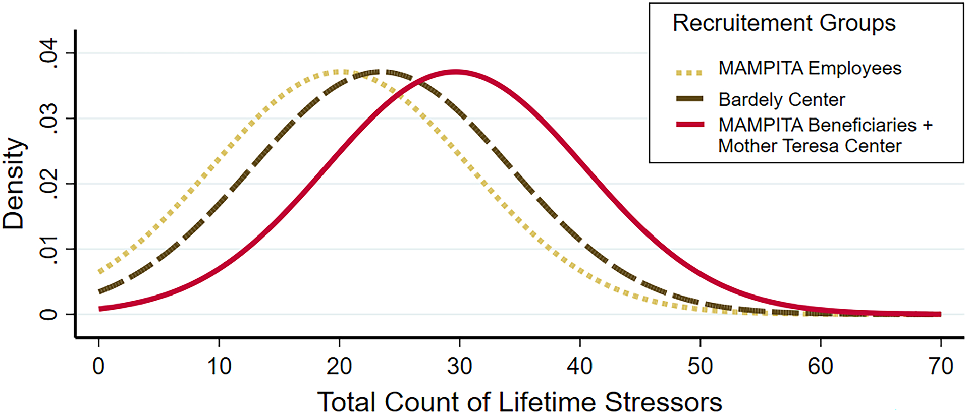
Each curve displays the inferred normal distribution of each recruitment group’s lifetime stressor count, with a common SD of 10.74 and their respective mean, according to the best fitted model selected by deviance reduction. MAMPITA beneficiaries and Mother Teresa Center beneficiaries (solid curve) had the same estimated mean of 29.65 lifetime stressor count. In contrast, Bardely Center participants (dashed curve) had an estimated mean of 23.46 lifetime stressor count and MAMPITA employees (doted curve) had an estimated mean of 20.12 lifetime stressor count.

In terms of the SES quartiles, lifetime stress exposure showed a clear stratification between SES Quartile 1 and SES Quartile 2 (common M = 30.20) vs. SES Quartile 3 and SES Quartile 4 (common M = 22.69), F(1,61) = 8.76, p = 0.0023, η² = 0.12, f² = 0.14, as did stress exposure occurring over the last 180 days for SES Quartile 1 and SES Quartile 2 (common M = 7.40) vs. SES Quartile 3 and SES Quartile 4 (common M = 3.14), F(1,61) = 29.02, p < 0.0001, η² = 0.32, f² = 0.47.

As expected, lifetime stressor count also differed for men and women, with a mean of 20.66 lifetime stressors (SD = 8.32) for men and 27.79 lifetime stressors (SD = 10.69) for women, t₆₁ = −1.88, p = 0.033, Hedges’ g* = 0.68. The same gender stratification was observed for stressors occurring over the last 180 days, with a mean stressor count of 2.66 (SD = 2.00) for men and 5.98 (SD = 3.47) for women, t₆₁ = −2.58, p = 0.007, Hedges’ g* = 1.

Distribution of Depressive Symptoms

The mean BDI-II score was 20.47 (Median = 17, SD = 10.17). Therefore, participants as a whole exhibited moderately severe depressive symptoms. Of these participants, 17 had minor symptom levels, 18 had mild levels, 13 had moderate levels, and 15 had severe levels (see Figure 2).

Figure 2. BDI-II scores and distributions for the four recruitment groups.

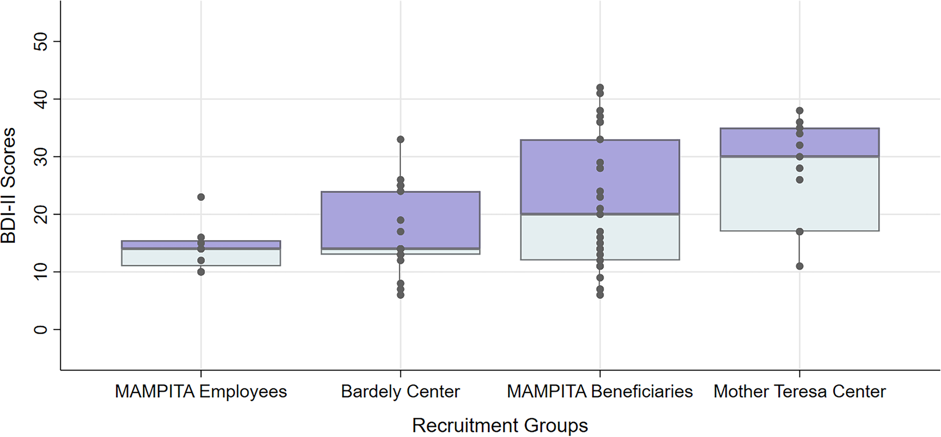
For each recruitment group, the data points and box plots indicate the distribution of participants’ BDI-II scores, revealing evidence that depression scores were socially stratified. MAMPITA employees all belonged to the upper socioeconomic stratum of the sample (i.e., university education, formal work contract, 100% in SES Quartile 4), whereas Mother Teresa Center beneficiaries were overwhelmingly part of the lowest stratum of the sample (i.e., primary education, never employed, mostly in SES Quartile 1). MAMPITA beneficiaries were among the most vulnerable participants in the sample (i.e., primary education, currently unemployed, mostly in SES Quartile 2 and SES Quartile 3), including indigent individuals (SES Quartile 1). Finally, Bardely Center participants spanned all of the SES strata, although they were slightly more represented in the two upper SES quartiles (i.e., primary education, mostly running an income generating activity, and in SES Quartile 3 and SES Quartile 4).

ANOVA models examining mean differences in depression scores across the recruitment groups revealed equal means for Mother Teresa Center participants and MAMPITA Beneficiaries, and for Bardely Center participants and MAMPITA Employees, respectively, but violated normality and/or homoscedasticity assumptions. The resulting mean values are therefore not reported, and we conducted non-parametric tests. First, a Kruskal-Wallis test validated the presence of significant mean differences in BDI-II scores across the groups, χ(3) = 10.366, p = 0.0158. Then, a Dunn test with unilateral hypothesis evidenced a significant mean difference in BDI-II scores between Mother Teresa Center and Bardely Center participants, Z = −2.70, p_Bonf = 0.026, and between Mother Teresa Center participants and MAMPITA Employees, Z = −2.77, p_Bonf = 0.017.

A second series of ANOVAs examining BDI-II mean differences across the SES quartiles showed a common mean of 15.35 for those in SES Quartile 1 and SES Quartile 2, and 24.57 for SES Quartile 3 and SES Quartile 4, respectively, F(1,61) = 15.94, p < 0.0001, η² = 0.20, f² = 0.25 (see Figure 3).

Figure 3. Distribution of depressive symptom (BDI-II) scores by self-reported SES quartiles.

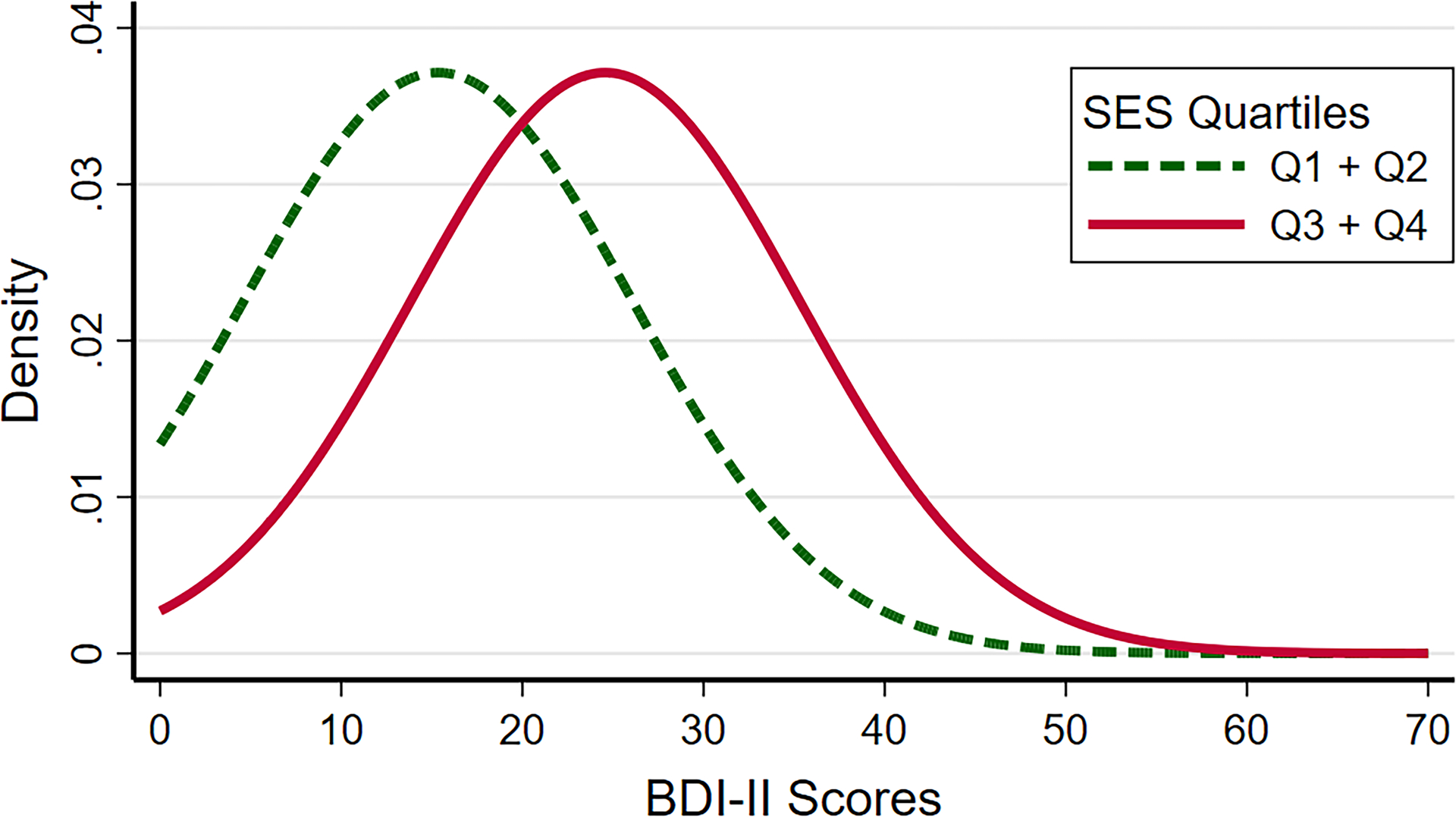
Each curve displays the inferred normal distribution of each SES quartile’s depressive symptom level as measured by the BDI-II, with a common SD of 10.17 and their respective mean, according to the best fitted model selected by deviance reduction. Self-reported SES Quartile 3 and SES Quartile 4 (solid curve) had the same estimated mean of 24.57, whereas self-reported SES Quartile 1 and SES Quartile 2 (dashed curve) had a mean of 15.35.

Consistent with prior research (e.g., Musliner et al., 2016), men and women differed in their depressive symptom severity in this LMIC population. On average, women exhibited moderate levels of depressive symptoms (M = 21.38, SD = 10.23), whereas men exhibited mild levels of depressive symptoms (M = 15, SD = 8.32), t₆₁ = −1.774, p = 0.041, Hedges’ g* = 0.64. An overview of the stratified distributions of life stress exposure and depressive symptoms across gender, recruitment group, and SES quartiles is provided in Table 4.

Table 4.

Exposure to stressors over the entire lifetime and last 180 days and BDI-II scores

Recruitment Groups	Lifetime stressor count M (SD)	Last 180 days stressor count M (SD)	BDI-II scores M (SD)
Mother Teresa Center	29.81 (10.53)	7.27 (4.64)	27.64 (8.96)
MAMPITA beneficiaries	29.59 (12.02)	6.40 (3.44)	21.78 (11.47)
Bardely Center	23.47 (7.00)	4.64 (3.19)	16.71 (7.55)
MAMPITA Employees	20.12 (9.62)	1.87 (1.45)	14.25 (4.17)
Socioeconomic Status Quartiles
SES Quartile 1	31.05 (11.70)	7.73 (3.60)	27.74 (10.10)
SES Quartile 2	29.18 (10.25)	7.00 (3.18)	22.00 (9.59)
SES Quartile 3	22.33 (8.69)	3.13 (2.87)	16.07 (10.37)
SES Quartile 4	22.69 (9.59)	3.15 (2.44)	14.54 (3.67)
Gender
Women	27.97 (10.69)	5.98 (3.74)	21.38 (10.23)
Men	20.66 (9.43)	2.66 (2.0)	15 (8.32)

Reported values are the empirical means and standard deviations of participants’ stressor count over the lifetime and over the last 180 days, and BDI-II scores.

Association between Lifetime Stress Exposure and Depressive Symptoms

The relation between participants’ lifetime stress exposure and depressive symptoms was explored using linear regressions. The best model of regression describing the relation between lifetime stressor count and BDI-II scores indicated that each stressor experienced increased participants’ BDI-II score by 0.42 points, F(1,61) = 15.09, R²_adj = 0.19, p = 0.00026, f² = 0.25. Given that participants experienced an average of 26.77 lifetime stressors, the average lifetime stress exposure burden in this sample contributed to an estimated BDI-II increase of 11.2 points.

Association between Stressor Type and Depressive Symptoms

The unique contribution of early vs. recent stressors composing this overall lifetime exposure was first analyzed with a stepwise regression model including stressors experienced during childhood, stressors experienced during adulthood, and stressors occurring over the last 180 days. In this model, childhood and adulthood stressors did not reach significance, whereas stressors occurring over the 180 last days were strongly associated with depressive symptoms, t = 5.38, p < 0.0001. Specifically, each additional stressor experienced was associated with a 1.55-point increase in participants’ BDI scores, F(1,61) = 28.96, R²_adj = 0.31, p < 0.0001, f² = 0.47.

However, refined regression models distinguishing the acute vs. chronic nature of the stressors occurring during the three aforementioned developmental periods (i.e., childhood, adulthood, last 180 days) displayed a more complex picture. Indeed, the best fit model, F(2,60) = 17.12, R²_adj = 0.3421, p < 0.0001, f² = 0.57, yielded two significant factors: each additional adulthood acute stressor was associated with a 0.28-point increase in participants’ BDI scores, t = 2.04, p = 0.046, and each additional chronic stressor occurring over the last 180 days was related to a 1.6-point increase in participants’ BDI scores, t = 3.79, p = 0.0004. Therefore, although both acute and chronic stressors were significantly associated with depression severity, these effects were especially strong for chronic stressors occurring recently. Chronic stressors experienced over the last 180 days and acute events experienced during adulthood—with a respective average of 4.43 and 14.09 in the present sample—contributed to an estimated BDI-II score increase of 11.09 points.

Mediation Analyses

Finally, we examined whether stress exposure mediated the association between gender and SES on depressive symptoms. In terms of the relation between gender and BDI-II scores, the NIE for lifetime stress exposure was significant (NIE = 2.809, p = 0.044, 95% CI [.32, 7.5]; see Figure 4), with stress accounting for 44.0% of the variability in the gender-depression association. In addition, adulthood acute stressors and chronic recent stressors had markedly significant indirect effects on depression (NIE = 3.68, p = .011, 95% CI [.91, 8.01] and ACME = 4.52, p = .001, 95% CI [1.65, 8.26], respectively), accounting for 57.6% and 70.8% of the association between gender and BDI-II, respectively. All paths exhibited full mediation.

Figure 4. Mediation diagram for the relation between socioeconomic status (SES score) and BDI-II score as mediated by lifetime stressor count.

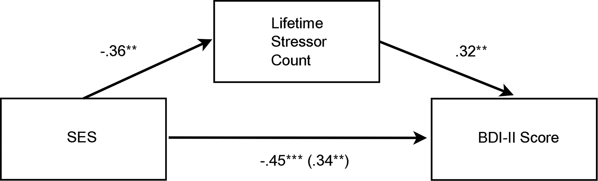
The predictor (SES score), mediator (Lifetime stressor count), and outcome (BDI-II score) are indicated by the three boxes. Arrows originating from these variables indicate their effect on the target variable. Beta standardized regression coefficients for these effects are shown next to the arrows, where ** = p < 0.001 and *** = p < 0.0001. The standardized regression coefficient between SES scores and participants’ depressive symptom (i.e., BDI-II) levels, controlling for lifetime stressor count, is shown in parentheses.

As for the association between SES and depression, every type of life stress exposure was a significant mediator and exhibited partial mediation. Lifetime stress exposure explained 25.7% of the variance in the SES-depression link (NIE = 2.36, p = .013, 95% CI [.54, 5.33]; see Figure 5), adulthood acute stressors explained 24% of the variance in the SES-depression link (NIE = 2.21, p = .01, 95% CI [.46, 5.05]), and chronic stressors occurring over the last 180 days explained 61.9% of the variance in the SES-depression link (NIE = 5.7, p < .0004, 95% CI [2.23, 9.77]).

Figure 5. Mediation diagram for the relationship between gender and BDI-II score as mediated by lifetime stressor count.

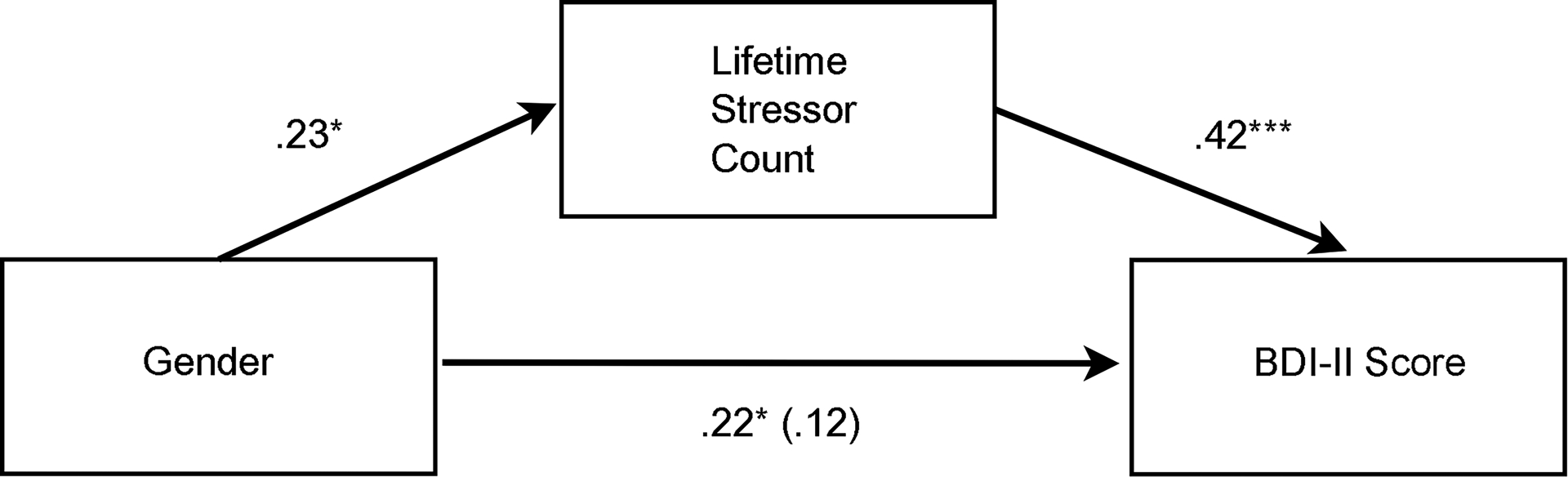
The predictor (Gender), mediator (Lifetime stressor count), and outcome (BDI-II score) are indicated by the three boxes. Arrows originating from these variables indicate their effect on the target variable. Beta standardized regression coefficients for these effects are shown next to the arrows, where * = p < 0.05 and *** = p < 0.0001. The standardized regression coefficient between gender and participants’ depressive symptom (i.e., BDI-II) levels, controlling for lifetime stressor count, is shown in parentheses.

Discussion

Although an abundance of research has examined associations between SES, gender, and life stress, the vast majority of these studies have been conducted in so-called WEIRD populations. We addressed this issue in the present study by interviewing adults living in Madagascar, which is a typical LMIC. We tested four main hypotheses: (a) SES and gender would be associated with the severity of participants’ lifetime stress exposure and depressive symptoms, (b) there would be a significant effect of lifetime stress exposure on the severity of participants’ depressive symptoms, (c) these effects would differ by the specific types of stressors experienced, and (d) stress exposure would mediate the association between gender and SES on depressive symptoms.

The data yielded four main results. First, we found a SES- and gender-related stratification of lifetime and recent stress exposure. On average, women experienced more life stressors occurring over both timeframes relative to men, as did those from lower vs. higher SES status groups. Likewise, we found a differential effect of gender on BDI-II scores, with women experiencing more severe depressive symptoms, on average, than men. This finding is consistent with many epidemiological studies that have reported gender-related differences in depressive symptoms (e.g., Hammen, 2003; Musliner, Munk-Olsen, Eaton, & Zandi, 2016; Salk, Hyde, & Abramson, 2017). Similarly, we found a differential effect of SES on depressive symptoms severity: the lower the SES strata (Mother Teresa Center participants and MAMPITA beneficiaries, for instance), the more severe the depressive symptoms. Considered together, the data provide robust evidence of an obstinately stratified distribution of lifetime stress exposure and depressive symptoms across SES strata and genders. These findings are consistent with the social determinants of health and social causation frameworks but extend this work to a representative sample of the Mahajanga population, which is a typical LMIC population that is rarely studied. These results are also consistent with developmental (Hartman & Belsky, 2018), neuroendocrine (Herman et al., 2016), and emotion research (Noël, Fevrier, & Deflandre, 2018) in highlighting how socially stratified factors such as life stress exposure affect mental health.

Second, we found that lifetime stress exposure as measured by the STRAIN was strongly associated with depressive symptoms as assessed by the BDI-II, with participants’ STRAIN scores alone explaining 19% of the variance in individuals’ depression severity (moderate effect size, f² = 0.25). Third, contrary to our hypotheses and prior research (Vogt, Waeldin, Hellhammer, & Meinlschmidt, 2016), early life stressors were not significantly associated with depression severity, which may be due to some study design-related limitations (see below). However, recent stress exposure was a robust predictor of depressive symptom severity, accounting for a full 31% of the variance in participants’ BDI scores, with a large effect size (f² = 0.47). A more detailed model examining the joint contributions of lifetime acute stressor and recent chronic stressor count revealed that these stressor types accounted for 34.5% of the variance in individuals’ BDI-II scores, with a strong magnitude of effect (f² = 0.57). Different stressors therefore contributed and interacted differently to influence depressive symptom severity. Finally, we found that the different types of life stress exposure assessed mediated the association between both gender and SES on participants’ depressive symptom scores.

One of the most important features of this research is the population studied. To move beyond the vast majority of existing stress and depression studies that have sampled WEIRD individuals, we collected data from a moderately to highly vulnerable LMIC population that is rarely studied. Interestingly, even in this population, which is relatively vulnerable as a whole, SES- and gender-related stratifications in life stress exposure and depressive symptoms were clearly present. Although we did not collect biological data, the strong association we observed between life stress exposure and depressive symptoms is consistent with the Social Signal Transduction Theory of Depression, which hypothesizes that major life stressors activate pro-inflammatory processes that promote depressive symptoms (Slavich & Irwin, 2014; Slavich & Sacher, 2019; Slavich et al., 2020). However, the present research extends this work to focus on SES and gender, thus contributing to our understanding of how life stress may deplete cognitive functions and degrade health in a manner that perpetuates poverty (Gałecki & Talarowska, 2018; Haushofer & Fehr, 2014; Lund & Cois, 2018; Lund et al., 2011, 2018; Yu, 2018). Additional research is needed to test these mediating mechanisms.

The results of the present study demonstrate the need to provide greater access to psychotherapy for LMIC populations and vulnerable migrants exposed to traumatizing conditions (Gezie et al., 2018). Community-based group therapy has proven effective in reducing depressive symptoms and improving socioeconomic conditions in rural Uganda (Bolton et al., 2003). Another promising approach is mindfulness meditation, which has been shown to reduce inflammation and depressive symptoms (Black, O’Reilly, Olmstead, Breen, & Irwin, 2015; Black & Slavich, 2016; Bower et al., 2014; Lopez-Maya, Olmstead, & Irwin, 2019; see Shields, Spahr, & Slavich, 2020). Regardless of the intervention type, it will be important to ensure that the strategy used is acceptable, accessible, affordable, and scalable in a setting and country with limited resources.

Strengths and Limitations

This study has several strengths. First, it provides rare insight into the relation between life stress exposure and depressive symptoms in an understudied population. Second, it uses the STRAIN, which is the only instrument specifically designed to systematically assess lifetime stress exposure. Third, the results are consistent with several theories of depression and permit an improved understanding of the nature and dynamics of poverty. Finally, the study addresses the “big picture” by including both structural factors (i.e., gender and SES inequalities) and proximal social-interpersonal factors (i.e., life stress exposure) to help understand risk for depression, which is a silent epidemic in LMICs.

This study also has several limitations. First, as participants were recruited from Mahajanga, Madagascar, further studies drawing from other populations are needed to test whether the results generalize to other LMICs as well as to non-LMICs. Second, notwithstanding the difficulty associated with recruiting participants in LMICs, the sample size was limited and included relatively few men and high-SES individuals. Third, depression severity was assessed using self-report, which has the advantage of being face valid but is not a substitute for clinician-based ratings of depression severity. Fourth, although the STRAIN has been shown to have excellent test-retest reliability (e.g., Slavich & Shields, 2018), it is a retrospective instrument and can be influenced by biases in reporting or remembering stressors. Fifth, we did not examine any resilience factors, such as social support or integration, which could have moderated the effects of stress on depression and helped reveal additional processes affecting who is most resilient/vulnerable for this disorder (Malat et al., 2017; Valderhaug & Slavich, 2020). Finally, given the cross-sectional nature of this study, the results are correlational and additional research is needed to address issues of directionality and causality, as well as to confirm the robustness of the associations observed. In particular, the mediation analyses are revealing and consistent with our a priori hypotheses, but these results are also based on cross-sectional data and should thus be viewed tentatively and interrogated further using longitudinal data collection and experimental approaches.

Conclusion

In conclusion, we found that lifetime stress exposure and severity were strongly related to depressive symptom levels in this LMIC, and that stress exposure levels were especially high for women and for those belonging to lower SES strata. In addition to supporting several theories of depression, these data provided evidence of an unequal distribution of lifetime stress exposure and depressive symptoms across gender and SES strata, which highlights a self-reinforcing cycle wherein the poor conditions in which LMIC populations live—which are marked by socioeconomic inequity and gender inequality—favor detrimental lifelong socioeconomic experiences (i.e., stress exposure) that make upward mobility difficult. The result is an apparent increased likelihood of experiencing more severe depressive symptoms, which can severely impair social and occupational functioning and ultimately hamper social, educational, and economic attainment: a perfect “poverty trap” that expands the notion of poverty far beyond material considerations.

References

- Adler NE, Boyce T, Chesney MA, Cohen S, Folkman S, Kahn RL, & Syme SL (1994). Socioeconomic status and health: The challenge of the gradient. American Psychologist, 49, 15–24. doi: 10.1037/0003-066x.49.1.15 [DOI] [PubMed] [Google Scholar]
- APA. (2013). Diagnostic and Statistical Manual of Mental Disorders (DSM-5) (5th ed.). Arlington, VA: American Psychiatric Association Publishing. [Google Scholar]
- Beck A, Steer R, & Brown G (1996). BDI-II, Beck depression inventory: Manual. San, Antonio, TX: Psychological Corp. [Google Scholar]
- Black DS, O’Reilly GA, Olmstead R, Breen EC, & Irwin MR (2015). Mindfulness meditation and improvement in sleep quality and daytime impairment among older adults with sleep disturbances. JAMA Internal Medicine, 175, 494–501. doi: 10.1001/jamainternmed.2014.8081 [DOI] [PMC free article] [PubMed] [Google Scholar]
- Black DS, & Slavich GM (2016). Mindfulness meditation and the immune system: A systematic review of randomized controlled trials. Annals of the New York Academy of Sciences, 1373, 13–24. doi: 10.1111/nyas.12998 [DOI] [PMC free article] [PubMed] [Google Scholar]
- Bloomfield K, Gmel G, Neve R, & Mustonen H (2001). Investigating gender convergence in alcohol consumption in Finland, Germany, the Netherlands, and Switzerland: A repeated survey analysis. Substance Abuse, 22, 39–53. doi: 10.1080/08897070109511444 [DOI] [PubMed] [Google Scholar]
- Bolen KA, & Pearl J (2013). Eight Myths About Causality and Structural Equation Models. In Morgan LM (Ed.), Handbook of Causal Analysis for Social Research. Handbooks of Sociology and Social Research (pp. 301–328). Dordrecht: Springer. doi: 10.1007/978-94-007-6094-3_15 [DOI] [Google Scholar]
- Bolton P, Bass J, Neugebauer R, Verdeli H, Clougherty KF, Wickramaratne P, … Weissman M (2003). Group interpersonal psychotherapy for depression in rural Uganda. JAMA, 289, 3117. doi: 10.1001/jama.289.23.3117 [DOI] [PubMed] [Google Scholar]
- Bonful HA, & Anum A (2019). Sociodemographic correlates of depressive symptoms: A cross-sectional analytic study among healthy urban Ghanaian women. BMC Public Health, 19. doi: 10.1186/s12889-018-6322-8 [DOI] [PMC free article] [PubMed] [Google Scholar]
- Bower JE, Crosswell AD, Stanton AL, Crespi CM, Winston D, Arevalo J, … Ganz PA (2014). Mindfulness meditation for younger breast cancer survivors: A randomized controlled trial. Cancer, 121, 1231–1240. doi: 10.1002/cncr.29194 [DOI] [PMC free article] [PubMed] [Google Scholar]
- Boyce WT, & Keating DP (2004). Should we intervene to improve childhood circumstances?. In Kuh D, Shlomo YB, & Ezra S (Eds.). A life course approach to chronic disease epidemiology (pp. 415–445). Oxford University Press. doi: 10.1093/acprof:oso/9780198578154.003.0018 [DOI] [Google Scholar]
- Brown GW, & Harris TO (1989). Life events and measurement. In Brown GW, & Harris TO (Eds.). Life Events and Illness (pp. 3–45). Guilford Press. EAN: 9780898627237 [Google Scholar]
- Burke KC, Burke JD, Regier DA, & Rae DS (1990). Age at onset of selected mental disorders in five community populations. Archives of General Psychiatry, 47, 511–518. doi: 10.1001/archpsyc.1990.01810180011002 [DOI] [PubMed] [Google Scholar]
- Cazassa MJ, Oliveira MDS, Spahr CM, Shields GS, & Slavich GM (2020). The Stress and Adversity Inventory for Adults (Adult STRAIN) in Brazilian Portuguese: Initial validation and links with executive function, sleep, and mental and physical health. Frontiers in Psychology, 10. doi: 10.3389/fpsyg.2019.03083 [DOI] [PMC free article] [PubMed] [Google Scholar]
- Cronkite RC, Moos RH, Twohey J, Cohen C, & Swindle R (1998). Life circumstances and personal resources as predictors of the ten-year course of depression. American Journal of Community Psychology, 26, 255–280. doi: 10.1023/a:1022180603266 [DOI] [PubMed] [Google Scholar]
- Diderichsen F, Evans T, & Whitehead M (2001). The Social Basis of Disparities in Health. In Evans T, Whitehead M, Diderichsen F, Bhuiya A, & Wirth M Challenging Inequities in Health: From Ethics to Action (pp. 12–23. Oxford University Press. doi: 10.1093/acprof:oso/9780195137408.003.0002 [DOI] [Google Scholar]
- Dura JR, Stukenberg KW, & Kiecolt-Glaser JK (1990). Chronic stress and depressive disorders in older adults. Journal of Abnormal Psychology, 99, 284–290. doi: 10.1037/0021-843x.99.3.284 [DOI] [PubMed] [Google Scholar]
- Evans GW, Li D, & Whipple SS (2013). Cumulative risk and child development. Psychological Bulletin, 139(6), 1342–1396. doi: 10.1037/a0031808 [DOI] [PubMed] [Google Scholar]
- Feurer C, McGeary JE, Knopik VS, Brick LA, Palmer RH, & Gibb BE (2017). HPA axis multilocus genetic profile score moderates the impact of interpersonal stress on prospective increases in depressive symptoms for offspring of depressed mothers. Journal of Abnormal Psychology, 126, 1017–1028. doi: 10.1037/abn0000316 [DOI] [PMC free article] [PubMed] [Google Scholar]
- Gałecki P, & Talarowska M (2018). Inflammatory theory of depression. Psychiatria Polska, 52, 437–447. doi: 10.12740/pp/76863 [DOI] [PubMed] [Google Scholar]
- Geyer S (2006). Education, income, and occupational class cannot be used interchangeably in social epidemiology. Empirical evidence against a common practice. Journal of Epidemiology & Community Health, 60, 804–810. doi: 10.1136/jech.2005.041319 [DOI] [PMC free article] [PubMed] [Google Scholar]
- Gezie LD, Yalew AW, Gete YK, Azale T, Brand T, & Zeeb H (2018). Socio-economic, trafficking exposures and mental health symptoms of human trafficking returnees in Ethiopia: Using a generalized structural equation modelling. International Journal of Mental Health Systems, 12, 1–13. doi: 10.1186/s13033-018-0241-z [DOI] [PMC free article] [PubMed] [Google Scholar]
- Gilman SE, Kawachi I, Fitzmaurice GM, & Buka L (2003). Socio-economic status, family disruption and residential stability in childhood: relation to onset, recurrence and remission of major depression. Psychological Medicine, 33, 1341–1355. doi: 10.1017/s0033291703008377 [DOI] [PubMed] [Google Scholar]
- Grzywacz JG, Almeida DM, Neupert SD, & Ettner SL (2004). Socioeconomic status and health: A micro-level analysis of exposure and vulnerability to daily stressors. Journal of Health and Social Behavior, 45, 1–16. doi: 10.1177/002214650404500101 [DOI] [PubMed] [Google Scholar]
- Hammen C (2003). Mood disorders. In Weiner IB, Stricker G, & Widiger TA (Eds.), Handbook of Psychology, Clinical Psychology (Vol. 8, pp. 93–118). Hoboken, New Jersey: John Wiley & Sons. [Google Scholar]
- Hammen C (2005). Stress and depression. Annual Review of Clinical Psychology, 1, 293–319. doi: 10.1146/annurev.clinpsy.1.102803.143938 [DOI] [PubMed] [Google Scholar]
- Hartman S, & Belsky J (2018). Prenatal programming of postnatal plasticity revisited—And extended. Development and Psychopathology, 30, 825–842. doi: 10.1017/s0954579418000548 [DOI] [PubMed] [Google Scholar]
- Haushofer J, & Fehr E (2014). On the psychology of poverty. Science, 344, 862–867. doi: 10.1126/science.1232491 [DOI] [PubMed] [Google Scholar]
- Herman JP, McKlveen JM, Ghosal S, Kopp B, Wulsin A, Makinson R, … Myers B (2016). Regulation of the hypothalamic-pituitary-adrenocortical stress response. Comprehensive Physiology, 6, 603–621. doi: 10.1002/cphy.c150015 [DOI] [PMC free article] [PubMed] [Google Scholar]
- Hoebel J, Maske UE, Zeeb H, & Lampert T (2017). Social inequalities and depressive symptoms in adults: The role of objective and subjective socioeconomic status. Plos One, 12, e0169764. doi: 10.1371/journal.pone.0169764 [DOI] [PMC free article] [PubMed] [Google Scholar]
- Holahan CJ, Moos RH, Holahan CK, Brennan PL, & Schutte KK (2005). Stress generation, avoidance coping, and depressive symptoms: A 10-year model. Journal of Consulting and Clinical Psychology, 73, 658–666. doi: 10.1037/0022-006x.73.4.658 [DOI] [PMC free article] [PubMed] [Google Scholar]
- James SL, Abate D, Abate KH, Abay SM, Abbafati C, Abbasi N, … Murray CJ (2018). Global, regional, and national incidence, prevalence, and years lived with disability for 354 diseases and injuries for 195 countries and territories, 1990–2017: A systematic analysis for the Global Burden of Disease Study 2017. The Lancet, 392, 1789–1858. doi: 10.1016/s0140-6736(18)32279-7 [DOI] [PMC free article] [PubMed] [Google Scholar]
- Judd LL (1997). The clinical course of unipolar major depressive disorders. Archives of General Psychiatry, 54, 989–991. doi: 10.1001/archpsyc.1997.01830230015002 [DOI] [PubMed] [Google Scholar]
- Judd LL, Akiskal HS, Zeller PJ, Paulus M, Leon AC, Maser JD, … Keller MB (2000). Psychosocial disability during the long-term course of unipolar major depressive disorder. Archives of General Psychiatry, 57, 375–380. doi: 10.1001/archpsyc.57.4.375 [DOI] [PubMed] [Google Scholar]
- Keller J, Gomez R, Williams G, Lembke A, Lazzeroni L, Murphy GM, & Schatzberg AF (2016). HPA axis in major depression: cortisol, clinical symptomatology and genetic variation predict cognition. Molecular Psychiatry, 22, 527–536. doi: 10.1038/mp.2016.120 [DOI] [PMC free article] [PubMed] [Google Scholar]
- Kendler KS, & Gardner CO (2016). Depressive vulnerability, stressful life events and episode onset of major depression: a longitudinal model. Psychological Medicine, 46, 1865–1874. doi: 10.1017/s0033291716000349 [DOI] [PMC free article] [PubMed] [Google Scholar]
- Lazarus RS, & Folkman S (1984). Stress, appraisal, and coping. New York: Springer. [Google Scholar]
- Lenze SN, Cyranowski JM, Thompson WK, Anderson B, & Frank E (2008). The cumulative impact of nonsevere life events predicts depression recurrence during maintenance treatment with interpersonal psychotherapy. Journal of Consulting and Clinical Psychology, 76, 979–987. doi: 10.1037/a0012862 [DOI] [PMC free article] [PubMed] [Google Scholar]
- Lépine JP & Briley M (2011). The increasing burden of depression. Neuropsychiatric Disease and Treatment, 7, 3–7. doi: 10.2147/ndt.s19617 [DOI] [PMC free article] [PubMed] [Google Scholar]
- Lopez-Maya E, Olmstead R, & Irwin MR (2019). Mindfulness meditation and improvement in depressive symptoms among Spanish- and English speaking adults: A randomized, controlled, comparative efficacy trial. Plos One, 14, e0219425. doi: 10.1371/journal.pone.0219425 [DOI] [PMC free article] [PubMed] [Google Scholar]
- Lorant V (2003). Socioeconomic inequalities in depression: A meta-analysis. American Journal of Epidemiology, 157, 98–112. doi: 10.1093/aje/kwf182 [DOI] [PubMed] [Google Scholar]
- Lund C, Brooke-Sumner C, Baingana F, Baron EC, Breuer E, Chandra P, … Saxena S (2018). Social determinants of mental disorders and the Sustainable Development Goals: A systematic review of reviews. The Lancet Psychiatry, 5, 357–369. doi: 10.1016/s2215-0366(18)30060-9 [DOI] [PubMed] [Google Scholar]
- Lund C, & Cois A (2018). Simultaneous social causation and social drift: Longitudinal analysis of depression and poverty in South Africa. Journal of Affective Disorders, 229, 396–402. doi: 10.1016/j.jad.2017.12.050 [DOI] [PubMed] [Google Scholar]
- Lund C, Silva MD, Plagerson S, Cooper S, Chisholm D, Das J, … Patel V (2011). Poverty and mental disorders: Breaking the cycle in low-income and middle-income countries. The Lancet, 378, 1502–1514. doi: 10.1016/s0140-6736(11)60754-x [DOI] [PubMed] [Google Scholar]
- Lupien SJ, King S, Meaney MJ, & McEwen BS (2000). Child’s stress hormone levels correlate with mother’s socioeconomic status and depressive state. Biological Psychiatry, 48, 976–980. doi: 10.1016/s0006-3223(00)00965-3 [DOI] [PubMed] [Google Scholar]
- Lupien SJ, King S, Meaney MJ, & McEwen BS (2001). Can poverty get under your skin? Basal cortisol levels and cognitive function in children from low and high socioeconomic status. Development and Psychopathology, 13, 653–676. doi: 10.1017/s0954579401003133 [DOI] [PubMed] [Google Scholar]
- Malat J, Jacquez F, & Slavich GM (2017). Measuring lifetime stress exposure and protective factors in life course research on racial inequality and birth outcomes. Stress, 20, 379–385. doi: 10.1080/10253890.2017.1341871 [DOI] [PMC free article] [PubMed] [Google Scholar]
- Malat J, Johns-Wolfe E, Smith T, Shields GS, Jacquez F, & Slavich GM (in press). Associations between lifetime stress exposure, race, and first-birth intendedness in the United States. Journal of Health Psychology. doi: 10.1177/1359105320963210 [DOI] [PMC free article] [PubMed] [Google Scholar]
- McLoughlin E, Fletcher D, Slavich GM, Arnold R, & Moore LJ (2021). Cumulative lifetime stress exposure, depression, anxiety, and well-being in elite athletes: A mixed-method study. Psychology of Sport and Exercise, 52, 101823. doi: 10.1016/j.psychsport.2020.101823 [DOI] [PMC free article] [PubMed] [Google Scholar]
- McMullin SD, Shields GS, Slavich GM, & Buchanan TW (in press). Cumulative lifetime stress exposure predicts greater impulsivity and addictive behaviors. Journal of Health Psychology. doi: 10.1177/1359105320937055 [DOI] [PMC free article] [PubMed] [Google Scholar]
- Monroe SM, & Slavich GM (2007). Psychological stressors, overview. In Fink G (Ed.), Encyclopedia of stress, second edition (Vol. 3, pp. 278–284). Oxford: Academic Press. [Google Scholar]
- Monroe SM, & Slavich GM (2016). Psychological stressors: Overview. In Fink G (Ed.), Stress: Concepts, cognition, emotion, and behavior, first edition (pp. 109–115). Cambridge, MA: Academic Press. doi: 10.1016/B978-0-12-800951-2.00013-3 [DOI] [Google Scholar]
- Monroe SM, & Slavich GM (2020). Major life events: A review of conceptual, definitional, measurement issues, and practices. In Harkness KL & Hayden EP (Eds.), The Oxford handbook of stress and mental health (pp. 7–26). New York: Oxford University Press. doi: 10.1093/oxfordhb/9780190681777.013.1 [DOI] [Google Scholar]
- Monroe SM, Slavich GM, & Georgiades K (2014). The social environment and depression: The roles of life stress. In Gotlib IH & Hammen CL (Eds.), Handbook of depression, third edition (pp. 296–314). New York: The Guilford Press. [Google Scholar]
- Monroe SM, Slavich GM, Torres LD, & Gotlib IH (2007). Major life events and major chronic difficulties are differentially associated with history of major depressive episodes. Journal of Abnormal Psychology, 116, 116–124. doi: 10.1037/0021-843X.116.1.116 [DOI] [PMC free article] [PubMed] [Google Scholar]
- Murray CJ, & Lopez AD (1996). The Global burden of disease: A comprehensive assessment of mortality and disability from diseases, injuries, and risk factors in 1990 and projected to 2020. World Bank and Harvard School of Public Health. Retrieved from https://apps.who.int/iris/handle/10665/41864 [Google Scholar]
- Murray CJ, Vos T, Lozano R, Naghavi M, Flaxman AD, Michaud C, … Lopez AD (2012). Disability-adjusted life years (DALYs) for 291 diseases and injuries in 21 regions, 1990–2010: A systematic analysis for the Global Burden of Disease Study 2010. The Lancet, 380, 2197–2223. doi: 10.1016/s0140-6736(12)61689-4 [DOI] [PubMed] [Google Scholar]
- Muscatell KA, Slavich GM, Monroe SM, & Gotlib IH (2009). Stressful life events, chronic difficulties, and the symptoms of clinical depression. The Journal of Nervous and Mental Disease, 197, 154–160. doi: 10.1097/nmd.0b013e318199f77b [DOI] [PMC free article] [PubMed] [Google Scholar]
- Musliner KL, Munk-Olsen T, Eaton WW, & Zandi PP (2016). Heterogeneity in long-term trajectories of depressive symptoms: Patterns, predictors and outcomes. Journal of Affective Disorders, 192, 199–211. doi: 10.1016/j.jad.2015.12.030 [DOI] [PMC free article] [PubMed] [Google Scholar]
- Noël Y (2018). R2STATS: A GTK GUI for fitting and comparing GLM and GLMM in R. R package version 0.68–39 Retrieved from http://CRAN.R-project.org/package=R2STATS
- Noël Y, Fevrier F, & Deflandre A (2018). Two factors but one dimension: An alternative view at the structure of mood and emotion. PsyArXiv. doi: 10.31234/osf.io/tv9ys [DOI] [Google Scholar]
- Pearl J (2014). Interpretation and identification of causal mediation. Psychological Methods, 19(4), 459–481. doi: 10.1037/a0036434 [DOI] [PubMed] [Google Scholar]
- Penley JA, Wiebe JS, & Nwosu A (2003). Psychometric properties of the Spanish Beck Depression Inventory-II in a medical sample. Psychological Assessment, 15, 569–577. doi: 10.1037/1040-3590.15.4.569 [DOI] [PubMed] [Google Scholar]
- R Core Team (2020). R: A language and environment for statistical computing. Vienna, Austria: R Foundation for Statistical Computing. Retrieved from https://www.R-project.org [Google Scholar]
- Rouder JN, Engelhardt CR, McCabe S & Morey RD (2016). Model comparison in ANOVA. Psychonomic Bulletin Review, 23, 1779–1786. doi: 10.3758/s13423-016-1026-5 [DOI] [PubMed] [Google Scholar]
- Salk RH, Hyde JS, & Abramson LY (2017). Gender differences in depression in representative national samples: Meta-analyses of diagnoses and symptoms. Psychological Bulletin, 143, 783–822. doi: 10.1037/bul0000102 [DOI] [PMC free article] [PubMed] [Google Scholar]
- Seedat S, Scott KM, Angermeyer MC, Berglund P, Bromet EJ, Brugha TS, … Kessler RC (2009). Cross-national associations between gender and mental disorders in the World Health Organization World Mental Health Surveys. Archives of General Psychiatry, 66, 785–795. doi: 10.1001/archgenpsychiatry.2009.36 [DOI] [PMC free article] [PubMed] [Google Scholar]
- Seiler A, von Känel R, & Slavich GM (2020). The psychobiology of bereavement and health: A conceptual review from the perspective of Social Signal Transduction Theory of Depression. Frontiers in Psychiatry, 11, 565239. doi: 10.3389/fpsyt.2020.565239 [DOI] [PMC free article] [PubMed] [Google Scholar]
- Sheets ES, & Craighead WE (2014). Comparing chronic interpersonal and noninterpersonal stress domains as predictors of depression recurrence in emerging adults. Behaviour Research and Therapy, 63, 36–42. doi: 10.1016/j.brat.2014.09.001 [DOI] [PMC free article] [PubMed] [Google Scholar]
- Shields GS, Spahr CM, & Slavich GM (2020). Psychosocial interventions and immune system function: A systematic review and meta-analysis of randomized clinical trials. JAMA Psychiatry, 77, 1031–1043. doi: 10.1001/jamapsychiatry.2020.0431 [DOI] [PMC free article] [PubMed] [Google Scholar]
- Slavich GM (2004). Deconstructing depression: A diathesis-stress perspective. Observer, 17, 15. [Google Scholar]
- Slavich GM (2016). Psychopathology and stress. In Miller HL (Ed.), The SAGE encyclopedia of theory in psychology, first edition (pp. 762–764). Thousand Oaks, CA: SAGE Publications. doi: 10.4135/9781483346274.n262 [DOI] [Google Scholar]
- Slavich GM (2019). Stressnology: The primitive (and problematic) study of life stress exposure and pressing need for better measurement. Brain, Behavior, and Immunity, 75, 3–5. doi: 10.1016/j.bbi.2018.08.011 [DOI] [PMC free article] [PubMed] [Google Scholar]
- Slavich GM (2020). Psychoneuroimmunology of stress and mental health. In Harkness KL & Hayden EP (Eds.), The Oxford handbook of stress and mental health (pp. 519–546). New York: Oxford University Press. doi: 10.1093/oxfordhb/9780190681777.013.24 [DOI] [Google Scholar]
- Slavich GM, & Auerbach RP (2018). Stress and its sequelae: Depression, suicide, inflammation, and physical illness. In Butcher JN & Hooley JM (Eds.), APA handbook of psychopathology: Vol. 1. Psychopathology: Understanding, assessing, and treating adult mental disorders (pp. 375–402). Washington, DC: American Psychological Association. doi: 10.1037/0000064-016 [DOI] [Google Scholar]
- Slavich GM, Giletta M, Helms SW, Hastings PD, Rudolph KD, Nock MK, & Prinstein MJ (2020). Interpersonal life stress, inflammation, and depression in adolescence: Testing Social Signal Transduction Theory of Depression. Depression and Anxiety, 37, 179–193. doi: 10.1002/da.22987 [DOI] [PMC free article] [PubMed] [Google Scholar]
- Slavich GM, & Irwin MR (2014). From stress to inflammation and major depressive disorder: A social signal transduction theory of depression. Psychological Bulletin, 140, 774–815. doi: 10.1037/a0035302 [DOI] [PMC free article] [PubMed] [Google Scholar]
- Slavich GM, O’Donovan A, Epel ES, & Kemeny ME (2010). Black sheep get the blues: A psychobiological model of social rejection and depression. Neuroscience & Biobehavioral Reviews, 35, 39–45. doi: 10.1016/j.neubiorev.2010.01.003 [DOI] [PMC free article] [PubMed] [Google Scholar]
- Slavich GM, & Sacher J (2019). Stress, sex hormones, inflammation, and major depressive disorder: Extending Social Signal Transduction Theory of Depression to account for sex differences in mood disorders. Psychopharmacology, 236, 3063–3079. doi: 10.1007/s00213-019-05326-9 [DOI] [PMC free article] [PubMed] [Google Scholar]
- Slavich GM, & Shields GS (2018). Assessing lifetime stress exposure using the Stress and Adversity Inventory for Adults (Adult STRAIN). Psychosomatic Medicine, 80, 17–27. doi: 10.1097/psy.0000000000000534 [DOI] [PMC free article] [PubMed] [Google Scholar]
- Slavich GM, Tartter MA, Brennan PA, & Hammen C (2014). Endogenous opioid system influences depressive reactions to socially painful targeted rejection life events. Psychoneuroendocrinology, 49, 141–149. doi: 10.1016/j.psyneuen.2014.07.009 [DOI] [PMC free article] [PubMed] [Google Scholar]
- Slavich GM, Thornton T, Torres LD, Monroe SM, & Gotlib IH (2009). Targeted rejection predicts hastened onset of major depression. Journal of Social and Clinical Psychology, 28, 223–243. doi: 10.1521/jscp.2009.28.2.223 [DOI] [PMC free article] [PubMed] [Google Scholar]
- Stoolmiller M, Kim HK, & Capaldi DM (2005). The course of depressive symptoms in men from early adolescence to young adulthood: Identifying latent trajectories and early predictors. Journal of Abnormal Psychology, 114, 331–345. doi: 10.1037/0021-843x.114.3.331 [DOI] [PMC free article] [PubMed] [Google Scholar]
- Sturmbauer SC, Shields GS, Hetzel E-L, Rohleder N, & Slavich GM (2019). The Stress and Adversity Inventory for Adults (Adult STRAIN) in German: An overview and initial validation. Plos One, 14, e0216419. doi: 10.1371/journal.pone.0216419 [DOI] [PMC free article] [PubMed] [Google Scholar]
- Tingley D, Yamamoto T, Hirose K, Keele L, Imai K (2014). “mediation: R Package for Causal Mediation Analysis.” Journal of Statistical Software, 59, 1–38, doi: 10.18637/jss.v059.i0526917999 [DOI] [Google Scholar]
- Turner RJ, Wheaton B, & Lloyd DA (1995). The epidemiology of social stress. American Sociological Review, 60, 104–125. doi: 10.2307/2096348 [DOI] [Google Scholar]
- Valderhaug TG, & Slavich GM (2020). Assessing life stress: A critical priority in obesity research and treatment. Obesity, 28, 1571–1573. doi: 10.1002/OBY.22911 [DOI] [PMC free article] [PubMed] [Google Scholar]
- Varghese FP, & Brown ES (2001). The hypothalamic-pituitary-adrenal axis in major depressive disorder: A brief primer for primary care physicians. Primary Care Companion to the Journal of Clinical Psychiatry, 3, 151–155. doi: 10.4088/pcc.v03n0401 [DOI] [PMC free article] [PubMed] [Google Scholar]
- Vinkers CH, Gastel W, Luykx JJ, Schubart C, Joëls M, Kahn RS, & Boks MP (2012). The effect of cumulative stress exposure on depressive symptoms is modified by a mineralocorticoid receptor haplotype. European Journal of Psychotraumatology, 3. doi: 10.3402/ejpt.v3i0.19460 [DOI] [Google Scholar]
- Vinkers CH, Joëls M, Milaneschi Y, Kahn RS, Penninx BW, & Boks MP (2014). Stress exposure across the life span cumulatively increases despression risk and is moderated by neurotism. Depression and Anxiety, 31, 737–745. doi: 10.1002/da.22262 [DOI] [PubMed] [Google Scholar]
- Vogt D, Waeldin S, Hellhammer D, & Meinlschmidt G (2016). The role of early adversity and recent life stress in depression severity in an outpatient sample. Journal of Psychiatric Research, 83, 61–70. doi: 10.1016/j.jpsychires.2016.08.007 [DOI] [PubMed] [Google Scholar]
- Vrshek-Schallhorn S, Stroud CB, Mineka S, Hammen C, Zinbarg RE, Wolitzky-Taylor K, & Craske MG (2015). Chronic and episodic interpersonal stress as statistically unique predictors of depression in two samples of emerging adults. Journal of Abnormal Psychology, 124, 918–932. doi: 10.1037/abn0000088 [DOI] [PMC free article] [PubMed] [Google Scholar]
- World Health Organization. (2010). Equity, Social Determinants and Public Health Programmes. Retrieved from https://apps.who.int/iris/handle/10665/44289v
- World Health Organization, Calouste Gulbenkian Foundation. (2014). Social determinants of mental health. Retrieved from https://apps.who.int/iris/bitstream/handle/10665/112828/9789241506809_eng.pdf?sequence=1
- World Health Organization. (2020). Depression Fact Sheet. Retrieved from https://www.who.int/en/news-room/fact-sheets/detail/depression
- Yu S (2018). Uncovering the hidden impacts of inequality on mental health: A global study. Translational Psychiatry, 8. doi: 10.1038/s41398-018-0148-0 [DOI] [PMC free article] [PubMed] [Google Scholar]