Sources and Risk Factors for Nitrate and Microbial Contamination of Private Household Wells in the Fractured Dolomite Aquifer of Northeastern Wisconsin

Abstract

Background:

Groundwater quality in the Silurian dolomite aquifer in northeastern Wisconsin, USA, has become contentious as dairy farms and exurban development expand.

Objectives:

We investigated private household wells in the region, determining the extent, sources, and risk factors of nitrate and microbial contamination.

Methods:

Total coliforms, Escherichia coli, and nitrate were evaluated by synoptic sampling during groundwater recharge and no-recharge periods. Additional seasonal sampling measured genetic markers of human and bovine fecal-associated microbes and enteric zoonotic pathogens. We constructed multivariable regression models of detection probability (log-binomial) and concentration (gamma) for each contaminant to identify risk factors related to land use, precipitation, hydrogeology, and well construction.

Results:

Total coliforms and nitrate were strongly associated with depth-to-bedrock at well sites and nearby agricultural land use, but not septic systems. Both human wastewater and cattle manure contributed to well contamination. Rotavirus group A, Cryptosporidium, and Salmonella were the most frequently detected pathogens. Wells positive for human fecal markers were associated with depth-to-groundwater and number of septic system drainfield within $229\mathrm{m}$. Manure-contaminated wells were associated with groundwater recharge and the area size of nearby agricultural land. Wells positive for any fecal-associated microbe, regardless of source, were associated with septic system density and manure storage proximity modified by bedrock depth. Well construction was generally not related to contamination, indicating land use, groundwater recharge, and bedrock depth were the most important risk factors.

Discussion:

These findings may inform policies to minimize contamination of the Silurian dolomite aquifer, a major water supply for the U.S. and Canadian Great Lakes region. https://doi.org/10.1289/EHP7813

Introduction

The paradox presented to the $13.1\text{\hspace{0.17em}million}$ households in the United States that rely on private wells for supplying their drinking water (NGWA 2020) is that the household owns the well and the land on which the well is constructed, but it does not control the source, movement, and quality of the pumped groundwater. Anthropogenic disturbances on neighboring properties, such as changes in land cover, building development, agricultural practices, septic systems, and groundwater withdrawals, can alter the supply and quality of groundwater on which the household depends. Thus, as a shared natural resource, groundwater is susceptible to the “tragedy of open access” (Bromley and Cernea 1989), where without appropriate institutional safeguards the resource (i.e., groundwater) can become diminished and degraded.

This tension of having competing land uses affect the shared groundwater resource is particularly noteworthy in northeastern Wisconsin, where both dairy farms and exurban development have expanded atop the underlying Silurian dolomite aquifer. The aquifer is the water source for at least 85% of private wells in the region (K. Bradbury, Wisconsin State Geologist, personal communication). In the region’s four main agricultural counties, Brown, Calumet, Kewaunee, and Manitowoc, the number of milking dairy cows increased from 132,558 to 180,860 between 2002 and 2017, a 36% increase (USDA NASS 2002, 2017). This number of milking cows produces approximately $5.9\times {10}^9$ kg of excrement (manure and urine) per year (Nennich 2005), which in northeastern Wisconsin is all applied to the landscape (Erb et al. 2015). Population growth in the four-county region between 1950 and 2000 increased exurbanization by as much as 60% (Brown et al. 2005). Dairy farms and exurban homes are in greater proximity than years ago, each land use potentially contributing to the degradation of the common groundwater resource on which they depend.

Compounding the effects of more intensive land use on groundwater quality is the highly vulnerable nature of the Silurian dolomite aquifer, which is an important water supply for the region (Figure 1). The dolomite bedrock is densely fractured in both horizontal and vertical directions, and in many regions the surficial sediment overlying the bedrock is thin, i.e., $6\mathrm{m}$ or less (Sherrill 1978). Groundwater recharge is extremely rapid because soil macropores and the extensive vertical fracture network allow rain and snowmelt water to infiltrate easily (Muldoon and Bradbury 2010). Infiltrating water carries contaminants originating at the land surface to the water table, after which groundwater flow in horizontal fractures can be rapid, providing little attenuation to contaminant transport (Bradbury and Muldoon 1992; Muldoon et al. 2001).

Figure 1.

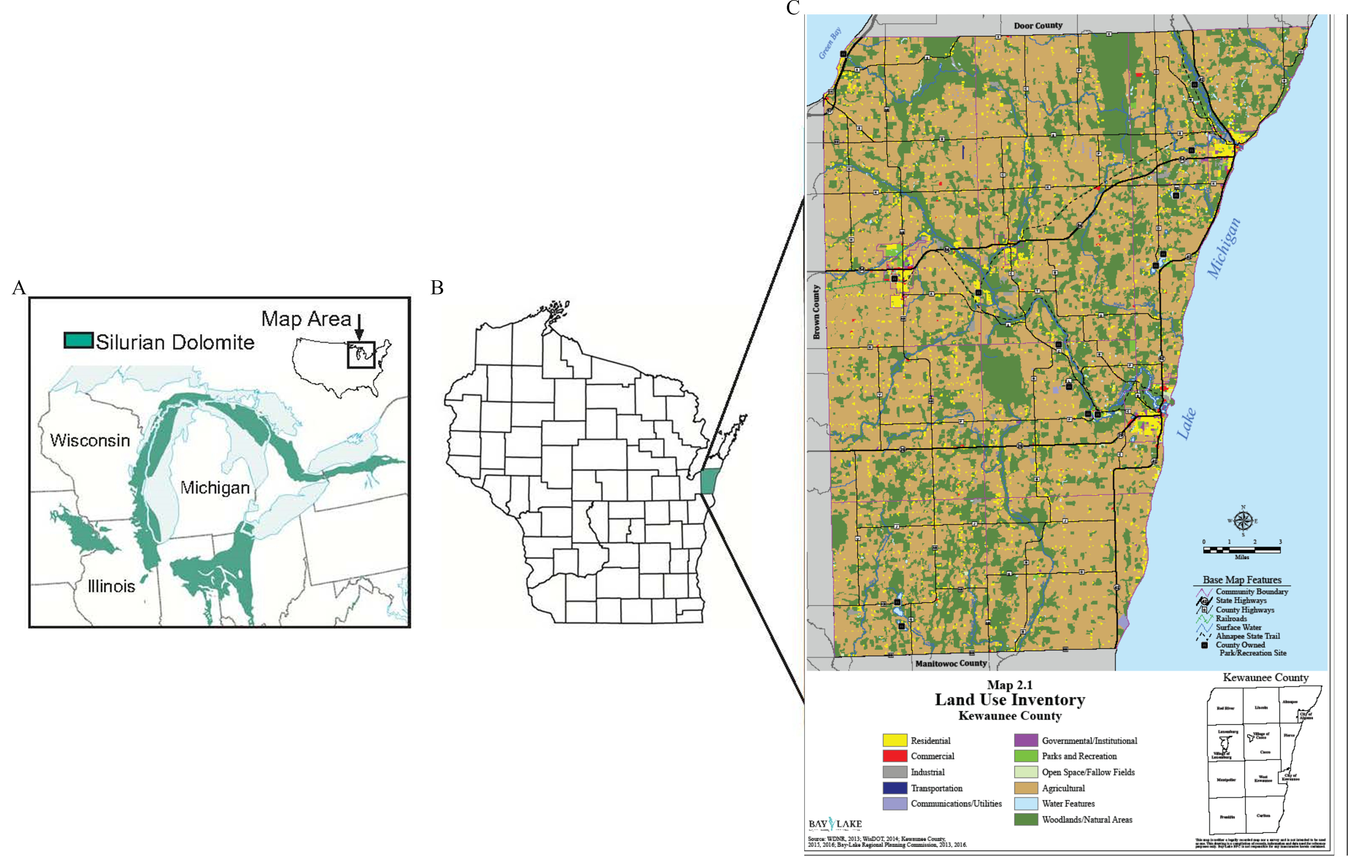
Location of study site including (A) map of generalized Silurian dolomite subcrop shown as shaded area (modified from Shaver et al. 1978); (B) location of Kewaunee County, Wisconsin, United States; and (C) map of land use within the county. Land use map reprinted with permission from Bay Lake Regional Planning Commission, Green Bay, Wisconsin.

Contamination of private household wells open to the Silurian dolomite aquifer has been evaluated primarily by standard indicator bacteria for water sanitary quality (i.e., total coliform bacteria and Escherichia coli) and nitrate–nitrogen (${\mathrm{NO}}_3^{-}\text{-N}$) In the five-county region where the aquifer is most vulnerable (Brown, Calumet, Door, Kewaunee, and Manitowoc Counties), 14% of 7,521 samples from private wells exceeded the U.S. Environmental Protection Agency (U.S. EPA) health advisory of $10\mathrm{mg}/\mathrm{L}$ for ${\mathrm{NO}}_3^{-}\text{-N}$ for public water supplies (U.S. EPA 2020). Twenty-three percent of 6,739 samples tested positive for total coliforms, and 2% of 6,583 samples were positive for E. coli (Center for Watershed Science and Education Wisconsin 2018). Although these analyses may indicate the extent of contamination, they do not provide information on the source of contamination.

The most obvious contamination events happen when manure enters the aquifer and is pumped from a household well into indoor taps as odoriferous brown water (Figure 2). Manure-containing brown water incidents are more likely during groundwater recharge when snow is melting and after dairy manure is applied to agricultural fields (Erb et al. 2015). Erb et al. (2015) documented 25 brown water incidents between 2008 and 2014 in domestic wells located in Brown, Calumet, Kewaunee, and Manitowoc counties, and these incidents can present a health risk (Wisconsin Department of Health Services n.d.).

Figure 2.

“Brown water” event at a Kewanee County household with a private well. Note: Photo provided and permission granted by Chuck Wagner.

As the “tragedy of open access” of the groundwater resource in northeast Wisconsin was unfolding, public debate centered on two questions: a) what is the true extent of groundwater contamination? and b) what are the sources of contamination, septic systems or dairy manure? Through interactions with stakeholders, we learned that historical total coliform and nitrate data were considered biased by some because it was believed samples were submitted only from problem wells that were not representative of groundwater conditions. As for the source question, opposing sides generally took positions without having data in hand, because the technology of microbial source tracking (MST) to identify fecal sources has rarely been applied to household wells. To help resolve these questions and bring information to bear on potential solutions, we proposed three study objectives: a) conduct random sampling of private wells, stratified by depth-to-bedrock, for indicator bacteria and nitrate; b) from the subset of wells in Objective 1 that were positive for total coliform bacteria or had ${\mathrm{NO}}_3^{-}\text{-}\mathrm{N}>10\mathrm{mg}/\mathrm{L}$, conduct random sampling for enteric pathogens and MST markers indicating whether fecal contamination was from septic systems or dairy manure; and c) perform statistical analyses to identify land use, weather, hydrogeology, and well construction risk factors that were associated with private well contamination.

Methods

Study Area

The study area was Kewaunee County located in northeast Wisconsin, USA (Figure 1). The county’s population is 20,600, of which 11,300 (55%) live in 4,900 rural homes served by septic systems and private wells (Bay Lake Regional Planning Commission 2016). Land cover in the $2808{\text{-km}}^2$ county is predominantly agriculture (63%), natural areas (29%), and residential (3%) (Bay Lake Regional Planning Commission 2016). Dairy farming and associated crop production are the primary agricultural activities. Cattle and calves number approximately 107,000 on 306 farms (USDA NASS 2017). The climate is continental, modified by the proximity of Lake Michigan, with precipitation (rain and snow) of $78\mathrm{cm}$ water per year (NOAA n.d.). Soils are medium- to fine-textured, underlain by Pleistocene glacial deposits; unconsolidated sediments vary in thickness from several centimeters to more than $30\mathrm{m}$ over the bedrock (Erb et al. 2015). Karst features such as open fractures are present, albeit many are covered with soil (Erb et al. 2015).

Indicator Bacteria and Nitrate

Private household wells were selected by stratified random sampling for tests of total coliforms (hereafter coliforms), E. coli, and nitrate. Candidate wells were identified from a list of property parcels that a) were not served by municipal water systems and b) had improvement values greater than USD $\$\mathrm{30,000}$, which indicated that a residence (and therefore private well) was likely present ($n=\mathrm{4,896}$). Parcels with mailing and property addresses that did not match were excluded to prevent confusion regarding sample location ($n=948$).

Water sampling was conducted during two synoptic events, 13–14 November 2015 and 29–30 July 2016. Strata were defined by depth-to-bedrock (i.e., the depth of unconsolidated sediment overlying bedrock at the well site) because earlier work suggested this parameter influenced groundwater contamination (Final Report of the Northeast Wisconsin Karst Task Force 2007). Using ArcMap software (version 10.3.1; ESRI), candidate wells were grouped into three strata based on an existing depth-to-bedrock map (Sherrill 1979): $<1.5\mathrm{m}$ ($n=269$), $1.5–6.1\mathrm{m}$ ($n=473$), and $>6.1\mathrm{m}$ ($n=\mathrm{3,206}$). (Depth-to-bedrock data were not available for individual wells at the time of well selection.) Letters inviting participation were mailed, and all willing well owners (approximately 50% of invitees) received a sampling kit. After accounting for unreturned kits, 323 and 401 private well samples were submitted for the fall and summer sampling events, respectively. Some wells (103) were sampled in both events (see Figure S1 for well recruitment, exclusion, and dropout). All study wells were completed in the Silurian dolomite or overlying sediment.

Samples were collected by well owners following written instructions to sterilize the sample tap with a flame for 15 s or by alcohol swab and run the water run for at least 5 min prior to filling two polypropylene bottles provided in the sampling kit. The $60\text{-mL}$ nitrate bottle contained $160\mathrm{\mu }\mathrm{L}$ of 96% sulfuric acid for preservation. Samples were collected on the scheduled dates and on the same day delivered to designated receiving locations in the county where they were transported that day on ice to the laboratory. Coliforms and E. coli were analyzed by Colilert Quanti-Trays (IDEXX) within 48 h of sample collection. Nitrate was measured on an AQ1 Discrete Analyzer (SEAL Analytical) by cadmium reduction and reaction with sulfanilamide in conjunction with N-(1-naphthylethylenediamine) dihydrochloride (Method $4500\text{-}{\mathrm{NO}}_3^{-}\mathrm{F}$; American Public Health Association 1995).

Microbial Source Tracking and Pathogen Occurrence

Wells positive for coliforms or with ${\mathrm{NO}}_3^{-}\text{-}\mathrm{N}>10\mathrm{mg}/\mathrm{L}$ were eligible for additional sampling to assess sources of fecal contamination and the occurrence of enteric pathogens. From this group, wells were selected for five sampling events: 18–22 April, 1–3 August, and 31 October–2 November in 2016 and 23–24 January and 27–29 March in 2017. For each event, selection was randomized and stratified by the three depth-to-bedrock categories. We sampled 22 to 30 wells during each event, resulting in 138 samples from 131 wells; seven wells were sampled in two events.

Sampling was conducted by trained staff using dead-end ultrafiltration (Smith and Hill 2009) with Hemodialyzer Rexeed-25s ultrafilters (Asahi Kasei Medical MT Corp.). Water taps were flame-sterilized before ultrafilter attachment; all ultrafilter tubing and fittings were new for each sample. Well water was collected prior to softening or other treatment systems. Mean sample volume was $839\mathrm{L}$ (range: $522–\mathrm{1,517}\mathrm{L}$, $n=138$). Ultrafilters were bagged, placed on ice, and back-flushed in the laboratory within 72 h.

Ultrafilters were back-flushed using a $500\text{-mL}$ solution containing 0.01% sodium polyphosphate (NaPP), 0.5% Tween 80, and 0.001% antifoam Y-30 (Smith and Hill 2009). Bacto beef extract (ThermoFisher Scientific Catalog No. 211520) was added to the back-flushed eluate at a 1% weight to volume ratio (typically $6.5\mathrm{g}$ of beef extract into $650\mathrm{mL}$ of eluate) to provide an organic matrix for sample archival at $-80°\mathrm{C}$ and to aid flocculation of the secondary concentration step by polyethylene glycol (PEG) flocculation (Lambertini et al. 2008). Briefly, samples were incubated overnight at 4°C following addition of 8% PEG 8,000 and $0.2\mathrm{M}$ NaCl. Samples were centrifuged for 45 min at $\mathrm{4,700}\times g$ at 4°C, and the pellet was resuspended in TE buffer to a final concentrated sample volume (FCSV) of $3–26\mathrm{mL}$ ($4\mathrm{mL}$ average). FCSVs were stored at $-80°\mathrm{C}$ until extraction of nucleic acids. Nucleic acids were extracted from $280\mathrm{\mu }\mathrm{L}$ of final concentrated sample volume with the QIAamp DNA blood mini kit and buffer AVL using a QIAcube® (Qiagen). Final volume of the nucleic acid suspension was $140\mathrm{\mu }\mathrm{L}$. Three extractions were performed per sample to produce sufficient template for all gene markers assayed.

Virus RNA was reverse-transcribed (RT) by adding $25.8\mathrm{\mu }\mathrm{L}$ nuclease-free water and $2.1\mathrm{\mu }\mathrm{L}$ random hexamers (ProMega) to $25.8\mathrm{\mu }\mathrm{L}$ of the extracted nucleic acids. This mixture was heated for 5 min at 95°C and then mixed with $96.3\mathrm{\mu }\mathrm{L}$ RT master mix consisting of the following components reported as final concentrations in the $150\mathrm{\mu }\mathrm{L}$ total reaction volume: $50\text{\hspace{0.17em}mM}$ Tris-HCl (pH 8.3), $75\text{\hspace{0.17em}mM}$ KCl, $3\text{\hspace{0.17em}mM}$ ${\text{MgCl}}_2$, $0.6\text{\hspace{0.17em}mM}$ dithiothreitol, $70\mathrm{\mu }\mathrm{M}$ of each deoxynucleoside triphosphate (ProMega), $1\mathrm{U}/\mathrm{\mu }\mathrm{L}$ RNasin® (ProMega), $0.5\mathrm{U}/\mathrm{\mu }\mathrm{L}$ SuperScript® III reverse transcriptase (Invitrogen Life Technologies). Reaction incubation was 42°C for 60 min followed by 5 min at 95°C and then held at 4°C until polymerase chain reaction (PCR) amplification.

Samples were analyzed by quantitative real-time polymerase chain reaction (qPCR) for 33 gene markers specific to 30 microbial taxa or groups (see Table S1). The microbes tested were all fecal-associated and, based on the biology of the microbe or validation studies reported in the scientific literature, placed in one of three host-specificity categories: human-specific, bovine- or ruminant-specific, and no host specificity. qPCR was performed with a LightCycler® 480 instrument (Roche Diagnostics) using the LightCycler 480 Probes Master kit for all markers except for human Bacteroides, which used TaqMan Environmental Master Mix 2.0® (Applied Biosystems). $\text{Six\hspace{0.17em}}\mathrm{\mu }\mathrm{L}$ extracted DNA or cDNA from reverse transcription was added to $14\mathrm{\mu }\mathrm{L}$ of master mix, producing a $20\text{-}\mathrm{\mu }\mathrm{L}$ reaction volume. Primers and hydrolysis probes (Integrated DNA Technology), and their concentrations are reported in Table S1. For all markers except human Bacteroides, thermocycling began at 95°C for 5 min followed by 45 cycles of 10 s at 95°C and 1 min at 60°C with ramp rates of 4.4 and 2.2°C per second, respectively. Thermocycling for human Bacteroides began at 95°C for 10 min followed by 45 cycles of 30 s at 95°C, 2 min at 56°C, and 1 min at 72°C with ramp rates of 2.2, 1.1, and 2.2°C per second, respectively. Two qPCR technical replicates were performed per marker. If both replicates were negative the result is reported as 0. If only one was positive, that concentration is reported. If both replicates were positive, the average concentration is reported.

To ensure laboratory contamination was absent (i.e., no false positives), we performed negative controls (i.e., no-template controls) of every gene marker for the extraction, reverse transcription, and qPCR steps for every batch of these process steps, and we tested for every marker in every batch of ultrafilter backflush solution. All tests had to be negative [i.e., no cycle quantification (Cq) value] for sample data to be accepted.

Inhibition was evaluated following the approach of Gibson et al. (2012), using as controls Hepatitis G virus RNA oligonucleotide (IDT) and G-lambda DNA (New England Biolabs) for reverse transcription and qPCR inhibition, respectively. Samples with Cq values of controls that increased two or more were considered inhibited. Twelve of 138 samples were qPCR-inhibited, requiring dilution with AE buffer (Qiagen).

Extraction positive controls were bovine herpes virus vaccine for DNA and bovine respiratory syncytial virus vaccine for RNA (both vaccines from Zoetis Inc.), the latter serving also as the reverse transcription positive control. qPCR positive controls were gBlocks® or Ultramers® (IDT) of each marker, with sequences modified to distinguish from wild type while maintaining the same guanine and cytosine content.

Standard curves were generated by serially diluting the positive controls in AE buffer with 0.02% bovine serum albumin, creating a concentration range of 1 to ${10}^6$ gene copies (gc)/reaction. Quantification cycle (${\mathrm{C}}_{\mathrm{q}}$) values were calculated using the second derivative maximum method and regressed against the decimal logarithm of marker concentration using the nonlinear function provided by the LightCycler® 480 software. Standard curve parameters and 95% limits of detection are reported in Table S2 and Table S3, respectively.

Samples positive by qPCR for rotavirus group A were further analyzed following the methods of Iturriza-Gómara et al. (2004) and Madadgar et al. (2015) to determine human and bovine G and P genotypes using seminested PCR assays targeting the VP7 and VP4 structural viral protein genes. In brief, nucleic acid extraction and reverse transcription were performed as described above. The first PCR amplified the VP7 or VP4 gene using VP7-F/VP7-R or Con-3/Con-2 primers, respectively. The $20\text{-}\mathrm{\mu }\mathrm{L}$ reaction contained $6\mathrm{\mu }\mathrm{L}$ of cDNA from reverse transcription, $14\mathrm{\mu }\mathrm{L}$ of Roche LightCycler 480 master mix, and $200\text{\hspace{0.17em}nM}$ of each primer. A separate seminested reaction was run for each human and bovine G- and P-type (19 type-specific reactions). For all seminested reactions, $2\mathrm{\mu }\mathrm{L}$ of amplicon from the first reaction were added to $18\mathrm{\mu }\mathrm{L}$ of master mix containing one of the initial primers and a type-specific primer at $200\text{\hspace{0.17em}nM}$ each for a final reaction volume of $20\mathrm{\mu }\mathrm{L}$. (See Table S4 for all primers and their concentrations and Table S5 for thermocycling conditions for each reaction.)

PCR products ($20\mathrm{\mu }\mathrm{L}$) were visualized by gel electrophoresis on 1.5% agarose gel (100 V for 90 min). A negative control and two positive controls [RotaTeq® vaccine-positive human fecal specimen and bovine CalfGuard® vaccine (Zoetis)] were included in each analysis batch along with the DNA ladder (ProMega). Gel bands matching specific genotypes were purified with illustra™ GFX PCR DNA and Gel Band Purification Kit (GE Healthcare), and identity was confirmed by sequencing. Direct sequencing of the amplicons was performed in both directions using the seminested reaction primers (see Table S4). We used the BigDye® Terminator V3.1 Cycle Sequencing Kit (Applied Biosystems) for the sequencing reaction, and the University of Wisconsin–Madison Biotechnology Center performed the reads on an ABI 3730xl DNA Analyzer. Consensus sequences were constructed with Lasergene (DNAStar) and submitted for identification using BLAST (National Center for Biotechnology Information, Bethesda, MD). Genotypes were used to classify all rotavirus group A detections as human or bovine for inclusion in human and bovine-specific outcome measures: G1P[8] and G10P[11] were considered human- and bovine-specific genotypes, respectively (Pitzer et al. 2011; Papp et al. 2013).

Samples positive for human-specific Bacteroides (HF183/BacR287; Green et al. 2014) or ruminant-specific Bacteroides (Rum-2-Bac; Mieszkin et al. 2010) were reanalyzed by PCR (676 bp amplicon) and sequencing, following the method of Bernhard and Field (2000), to confirm Bacteroides identity. Bacteroides DNA was extracted by the method described above and $6\mathrm{\mu }\mathrm{L}$ DNA extract was added to $14\mathrm{\mu }\mathrm{L}$ LightCycler 480 Probes Master including $500\text{\hspace{0.17em}nM}$ of primers Bac32F and Bac708R (Bernhard and Field 2000). PCR commenced at 94°C for 5 min followed by 35 cycles consisting of 94°C for 30 s, 53°C for 1 min, and 72°C for 2 min, followed by a final 6-min extension at 72°C. PCR product ($10\mathrm{\mu }\mathrm{L}$) was visualized on 1.5% agarose gel. If the amplicon band was absent or faint, sensitivity was increased by reamplifying 1–$6\mathrm{\mu }\mathrm{L}$ of amplicon under the same thermocycling conditions. Product purification from the gel, the sequencing reaction, and analyses were performed as described above for rotavirus A genotyping. Direct sequencing of the amplicons was performed in both directions using primers 32F and 708R.

Risk Factor Variables

Well construction variables were obtained from well driller reports filed at the Wisconsin Geological and Natural History Survey or Wisconsin Department of Natural Resources. Reports were available for 65% of sampled wells. As described above, initial well selection was stratified using existing depth-to-bedrock maps. However, for the statistical analyses, the exact depth-to-bedrock value for each well was obtained from its construction report. When a report was not available ($n=116$ and 135 for fall and summer sampling events, respectively), bedrock depth was estimated by interpolation from reports of nearby wells. Well elevation was obtained from the county digital elevation model.

Groundwater depth was measured continuously in U.S. Geological Survey monitoring well KW-183 (USGS 443535087345401 KW-25/24E/34-0183) and data are available in the USGS National Water Information System (USGS 2020). The well is located in Kewaunee County near an agricultural field. Relative to the ground surface, depth-to-bedrock is $2.1\mathrm{m}$, borehole depth is $9.14\mathrm{m}$, and casing depth is $3.05\mathrm{m}$ (Muldoon and Bradbury 2010).

Groundwater recharge was estimated by the water table fluctuation method (Healy and Cook 2002), using graphical extrapolation of the antecedent recession curve and a specific yield of 0.04 based on previous assessments of recharge in the fractured rock in this area (Bradbury and Muldoon 1992). Cumulative recharge was obtained by summing individual recharge events for the 2-, 7-, 14-, and 21-d periods preceding sample collection.

Quantitative precipitation estimates (QPE) for each sampled well location (in $4\text{-km}$ grids) were provided by the North Central River Forecast Center of the U.S. National Weather Service. Because QPE values include snow, and frozen snow will not infiltrate soils, we excluded precipitation measurements for all well locations for days when snow without rain was recorded at the nearby National Weather Service station in Green Bay, Wisconsin. Cumulative precipitation was calculated by summing hourly QPE values over 2, 7, 14, and 21 d prior to sampling. Precipitation was not included in analyses of coliform and nitrate data because the synoptic design precluded variation in precipitation over the short time samples were collected.

Geographic Information System (GIS) data layers maintained by the Kewaunee County government reported locations of septic systems, agricultural fields, manure storages, and surface bedrock features. Agricultural field data included whether the field had a nutrient management plan (NMP) and therefore likely received manure applications.

Septic systems were divided into three categories for analysis: a) septic systems, included active systems of all types; b) drainfield, included inspected and uninspected systems that are designed to release effluent to the subsurface (i.e., excludes holding tanks); and c) not inspected, included only those systems that had not been inspected by county staff. Systems not in use were excluded from all three categories. The risk factor “distance to nearest septic system” excluded the system on the same property as the well, whereas counts of septic systems included the system on the same property.

Using ArcMap and Python script, fecal contamination sources and bedrock features were enumerated for each study well in two forms: a) distance from the well to the nearest contamination source or bedrock feature; and b) the count or areal size of the source or feature within three circular areas surrounding the well. The circular areas were defined by three radii from the well: 229, 457, and $914\mathrm{m}$ (equal to 750, 1,500, and 3,000 ft, respectively), corresponding to 16, 66, and 262 ha (approximately 40, 160, and 640 acres). These area sizes were selected prior to data analysis based on an earlier study of septic system counts in similar-sized areas that were associated with childhood infectious diarrhea (Borchardt et al. 2003a).

Statistical Analyses

Stratified random sampling was employed to generate estimated contamination rates of coliforms, E. coli, and nitrate. Sampling strata were defined by depth-to-bedrock ($<1.5$, 1.5–6.1, and $>6.1\mathrm{m}$). Smaller strata were oversampled relative to a simple random sample. This approach, in conjunction with the use of corresponding analytic weights and finite population correction factors in the analyses, resulted in more precise estimates for the smaller depth-to-bedrock strata without sacrificing the ability to estimate a countywide contamination rate. The analytic weight was defined as the product of the inverse of the sampling probability and the inverse of the response rate (i.e., the proportion of sampled well owners who agreed to participate in the study) within the appropriate depth-to-bedrock stratum. Rao-Scott likelihood ratio chi-square tests (Lohr 2010) were used to test associations between contamination rates and depth-to-bedrock as well as compare fall 2015 (groundwater recharge period) and summer 2016 (no recharge period) estimated contamination rates, both overall and within depth-to-bedrock strata. Statistical computations accounted for the complex sampling design.

Risk factors for well contamination were evaluated for independent variables relating to land use, precipitation, hydrogeology, bedrock, and well construction. Variables were tested for association with a) well contaminant detection and b) well contaminant concentration (among wells where contaminants were detected). Five contaminants (or contaminant groups) were tested for associations with risk factors: coliform bacteria, nitrate, human fecal markers, bovine fecal markers, and any fecal marker. Tests for coliform bacteria and nitrate associations were performed for each sampling period, groundwater recharge and no recharge.

For dichotomous (detect/nondetect) dependent variables, univariable screening for inclusion in the multivariable modeling process was performed using logistic regression. Each independent variable was represented as a linear (in the logit) term in the models. For independent variables with $>10\%$ zero values, a dichotomous (zero vs. greater than zero) term was included in the screening model in addition to the linear term. A plot of the estimated detection probability across the observed range of values for the independent variable being evaluated was also generated as part of the screening process. The same univariable screening process was performed for the well contaminant concentration dependent variables except that gamma regression with a natural log link function was used (Garson 2013), the model terms were linear in the log, and plots of estimated mean concentrations were generated.

For both univariable and multivariable analyses, outliers were excluded from the models for some of the concentration dependent variables. Specifically, 4 and 11 outliers were excluded from the analyses of coliform concentration for groundwater recharge and no recharge periods, respectively. And one, two, and four outliers were excluded for human, bovine, and any fecal marker concentration models, respectively. The criterion for excluding data points from the analyses was that their inclusion in the model caused the fitted curve to deviate meaningfully from the pattern exhibited by the remaining data. Concentration values for outliers were generally orders of magnitude larger than those in the remaining data points.

To be included in the multivariable model for a particular dependent variable, risk factors had to meet several criteria: a) strength of association (i.e., $p\le 0.15$); b) plausibility, the association had to be biologically or physically possible; and c) internal consistency, where variables of the same measurement but at different levels (e.g., count of septic system drainfields within 229, 457, or $914\mathrm{m}$ of a well) had similar directions of association (positive or negative) and strengths of association. When two variables of different measurements (e.g., well elevation and depth to bedrock) were correlated, the variable that most satisfied criteria 1, 2, and 3 was selected.

Additional screening was applied for inclusion in multivariable modeling when risk factors of the same measurement but at different levels were all associated with well contamination. Levels could differ in time (2, 7, 14, or 21 d) or area (within 229, 457, or $914\mathrm{m}$ from a well). Under this situation, the risk factor with the greatest strength of association was selected. For example, 2-, 7-, and 14-d cumulative precipitation variables were all strongly associated with well contamination of human-specific markers. However, the 2-d cumulative precipitation variable had the largest regression coefficient and lowest p-value, so it was selected for inclusion.

Once the independent variables for a given multivariable model were identified, a screening process for interaction terms among these variables was undertaken. Only interactions deemed plausible and relevant were assessed. A screening model contained a term for the interaction and main effect terms for the individual risk factors comprising the interaction. As with the univariable screening of main effects, the independent variables comprising the interaction were represented as linear terms in the models; an interaction term was included in the multivariable model when its p-value was $\le 0.15$.

For multivariable analyses, the same procedure was used for both well contaminant detection and well contaminant concentration. Gamma regression was employed for all multivariable analyses of well contaminant concentration. Prior to performing multivariable regression analyses, each independent variable retained after the screening process was reassessed at the univariable level to establish whether a more complex representation than linear (e.g., quadratic or spline) would be appropriate in the multivariable model. To decide on an appropriate representation, a plot of the logit of the detection probability (log of the mean concentration) across the observed range of values for the independent variable was generated and examined, with the independent variable represented as a natural cubic spline (Hastie et al. 2001) in the corresponding logistic (or gamma) regression model. If a more complex representation was deemed appropriate, it was used in both main effect and interaction terms in the multivariable models.

All risk factors and interaction terms retained after the above screening processes were included in each final multivariable model. We did this in order that the independent effects of each risk factor could be evaluated in the presence of (i.e., adjusting for) the other model terms.

The final multivariable models were fit using log-binomial (or gamma) regression to facilitate interpretation of the results (McNutt et al. 2003). These models permit direct estimation of ratios of detection probabilities (or mean concentrations). This is in contrast to logistic regression models, which estimate ratios of odds rather than probabilities. When presence of the dependent variable is not rare (roughly $<10\%$), which is typical in studies of well contaminant detection, the odds ratio does not closely approximate the corresponding ratio of detection probabilities and must be interpreted with caution.

For each multivariable model, procedures specific to generalized linear models were used to determine whether the information matrix was ill-conditioned (http://support.sas.com/kb/32/471.html). This approach entailed examining whether collinearity in the weighted risk factors was present, where the weights were determined by the model fitting algorithm.

Separate multivariable models for well construction risk factors were created because a number of wells were missing well construction reports. Had all risk factors been combined into a single model, only those wells without missing construction data would have been included, reducing statistical power to evaluate the other risk factors.

SAS version 9.4 was used to conduct all analyses (SAS Institute Inc.).

Results and Discussion

Groundwater Levels during Sampling

Groundwater levels during the first study year followed the pattern typical for the upper Midwest with rising levels in the fall and spring and falling levels in the summer and winter (Figure 3). However, there was a prolonged recharge period from fall 2016 to spring 2017 (Figure 3). In January 2017, snowmelt raised groundwater levels during a long warm period (NOAA n.d.). Coliform and nitrate sampling corresponded with fall recharge (hereafter “recharge”) and with the summer decline when groundwater was at nearly its deepest level (hereafter “no recharge”). Sampling for microbial source tracking occurred during recharge (3 events) and no-recharge (2 events) periods.

Figure 3.

Sampling periods in relation to groundwater level in Kewaunee County monitoring well KW-183 (USGS 443535087345401; USGS 2020). Sampling times indicated by red circles (total coliforms and nitrate) and green triangles (pathogens and fecal indicators). Boxes indicate the number of wells positive for human-specific or bovine-specific markers; $n=\text{total number of wells sampled}$. Gray shaded areas designate seasonal manure application ban for fields with bedrock depths $<6.1\mathrm{m}$.

Bacteria and Nitrate Contamination Rates

The countywide private well contamination rates for coliforms, E. coli, and ${\mathrm{NO}}_3^{-}\text{-N}>10\mathrm{mg}/\mathrm{L}$ were similar to the average rates for the state of Wisconsin (Table 1). However, for wells in the two shallowest bedrock depth strata ($<1.5\mathrm{m}$ and $1.5–6.1\mathrm{m}$), contamination rates were generally greater than the statewide averages, and rates were consistently greater than rates for wells in the deepest stratum ($>6.1\mathrm{m}$ to bedrock). The greater the bedrock depth and transport distance through surficial sediments, the less likely these contaminants will reach bedrock fractures that allow rapid transport (Final Report of the Northeast Wisconsin Karst Task Force 2007; Rasmuson et al. 2020).

Table 1.

Estimated contamination rates (percent positive wells) for total coliform bacteria, Escherichia coli, or $\text{nitrate-N}>10\mathrm{mg}/\mathrm{L}$.

Sampling period or reference data	Region or depth-to-bedrock categorya	Number of wells sampled	Percent positive wells (95% confidence interval)
			Total coliforms	E. coli	$\text{Nitrate-N}>10\mathrm{mg}/\mathrm{L}$	Total coliforms or nitrate-$\mathrm{N}>10\mathrm{mg}/\mathrm{L}$
Groundwater recharge	$<1.5\mathrm{m}$ to bedrock	26	46 (30, 63)	4 (0, 9)	7 (0, 15)	50 (34, 66)
	$1.5–6.1\mathrm{m}$ to bedrock	120	28 (18, 37)	1 (0, 2)	20 (7, 33)	42 (28, 55)
	$>6.1\mathrm{m}$ to bedrock	167	19 (11, 26)	0.3 (0, 0.6)	6 (1, 10)	23 (15, 31)
	Kewaunee County	313b,c 316c,d	21 (14, 27)	0.4 (0.1, 0.7)	7 (3, 11)	26 (19, 34)
No groundwater recharge	$<1.5\mathrm{m}$ to bedrock	24	23 (6, 39)	7 (0, 15)	10 (0, 20)	33 (12, 53)
	$1.5–6.1\mathrm{m}$ to bedrock	122	29 (16, 41)	1 (0, 3)	19 (9, 28)	40 (28, 53)
	$>6.1\mathrm{m}$ to bedrock	252	21 (15, 27)	1 (0, 2)	5 (2, 8)	26 (19, 32)
	Kewaunee County	396b,c 400c,d	22 (17, 28)	1 (0.1, 2)	7 (4, 10)	28 (22, 33)
Reference data	Wisconsine	534	23	3	7	—
	Wisconsinf	3,838	18	—	10	—

Note: —, no data available. Estimates and corresponding 95% confidence intervals account for the stratified random sampling design employed in the study.

^aThe estimated number of wells in each bedrock depth category are 76, 575, and 4,156 wells at $<1.5$, 1.5–6.1, and $>6.1\mathrm{m}$, respectively, totaling 4,807 wells in Kewaunee County. Our final estimates of the number of wells in each bedrock depth category are different than the initial estimates at the study beginning using the bedrock map created by Sherrill (1979).

^bn for coliforms and E. coli.

^cThe n’s do not equal the number of samples analyzed (see Figure S1) because some wells had missing depth-to-bedrock values (six wells for the groundwater recharge period and one well for the no recharge period) for which analytic weights could not be generated.

^dn for nitrate.

^eData for private wells; U.S. General Accounting Office 1997.

^fKnobeloch et al. 2013.

Groundwater recharge and no-recharge periods did not have significantly different contamination rates, regardless of contaminant type or level of data aggregation (Table 1). There was one exception; coliform contamination during recharge was greater than the no-recharge period for wells with bedrock depths $<1.5\mathrm{m}$ ($p=0.042$).

Table 2 reports descriptive statistics for coliforms, E. coli, and nitrate-N concentrations of positive samples. In both recharge and no-recharge periods, 25% of wells positive for nitrate-N had concentrations greater than $9\mathrm{mg}/\mathrm{L}$.

Table 2.

Descriptive statistics of coliform bacteria, Escherichia coli, and nitrate concentrations.

Sampling period	Measurement	Number of positive samples	Number of non-detects	Concentration of positive samplesa
				Mean	Median	Minimum	25th percentile	75th percentile	Maximumb
Groundwater recharge	Coliforms	87	232	73.2	5.2	1.0	2.0	17.3	$>\mathrm{2,419.6}$
	E. coli	5	314	5.0	2.0	1.0	2.0	4.1	16.1
	Nitrate-N	203	119	6.3	4.7	0.2	1.6	9.0	29.7
No groundwater recharge	Coliforms	87	310	116.8	6.2	1.0	2.0	55.4	$>\mathrm{2,419.6}$
	E. coli	10	387	105.0	3.1	1.0	1.3	8.8	1011.2
	Nitrate-N	205	196	6.5	5.2	0.2	2.1	9.1	33.3

Note: MPN, most probable number.

^aColiforms and E. coli, $\text{MPN}/100\mathrm{mL}$; nitrate-N, mg/L.

^b2,419.6 $\text{MPN}/100\mathrm{mL}$ was the upper limit of quantification.

Coliforms, although nonpathogenic, are the standard indicator of drinking-water sanitary quality in the United States. Studies of coliform-positive private wells have observed (DeFelice et al. 2016) and not observed (Strauss et al. 2001) associations with acute gastrointestinal illness. High nitrate in drinking water can cause methemoglobinemia, and in some studies it has been linked with colorectal cancer, thyroid disease, and central nervous system birth defects (Ward et al. 2018). The U.S. National Primary Drinking Water Standards apply only to public water systems, not private wells. Nonetheless, the U.S. drinking water Maximum Contaminant Level Goals (MCLG) for coliforms and nitrate-N provide public health benchmarks, which are zero and $10\mathrm{mg}/\mathrm{L}$, respectively (U.S. EPA 2020). Multiplying the MCLG exceedance rates for coliforms or nitrate-N (Table 1) by the estimated number of wells in each bedrock depth category in Kewaunee County [76, 575, and 4,156 wells at $<1.5$, 1.5–6.1, and $>6.1\mathrm{m}$, respectively (Borchardt et al. 2019)], we estimate approximately 1,300 wells (27%) during the study period did not meet U.S. EPA public health goals for safe drinking water.

Calculating well contamination rates by county, state, or other governmental units has the advantage of matching policy-making jurisdictions. However, aggregating data in this manner can overlook factors underlying contamination “hotspots,” in this case, bedrock depth. For example, the statewide averages for coliform and nitrate MCLG exceedances in Wisconsin, irrespective of bedrock depth, are 18% and 10%, respectively (Knobeloch et al. 2013). Using the multivariable models for coliforms and nitrate for recharge and no-recharge periods, respectively (see below and Figures 4B and 4C), the statewide percentages are equivalent to detection probabilities at bedrock depths of $10\mathrm{m}$ (coliforms) and $14\mathrm{m}$ (nitrate) in Kewaunee County. We estimate the number of wells with shallower bedrock depths, and therefore higher detection probabilities than the statewide averages, to be 1,562 (coliforms) and 2,464 (nitrate), which is 32% and 50% of the county’s private wells. This assessment is consistent with the high rates of coliform and nitrate exceedances for carbonate aquifers (e.g., Silurian dolomite) and agricultural areas observed in private well data nationally (DiSimone 2009).

Figure 4.

Detection probabilities for ${\mathrm{NO}}_3\text{-N}>10\mathrm{mg}/\mathrm{L}$ and coliform bacteria in private wells regressed (log-binomial) on key risk factors during groundwater recharge and no recharge periods. Coefficients and p-values are reported in Table 4. Black line: estimated probability of detection. Dashed lines: 95% pointwise confidence limits. Covariates in the multivariable models were fixed at their median values for the purpose of plotting. Fields with NMPs likely receive manure and inorganic fertilizer inputs. Note: NMP, nutrient management plan.

Microbial Source Tracking and Pathogen Occurrence

Of 138 samples from 131 wells, 82 samples (59%) from 79 wells (60%) were positive for markers of fecal-associated microbes (Table 3). Among the 79 wells with fecal contamination, 32 wells had markers for pathogens that could infect humans (human-specific and zoonotic pathogens without host specificity). Seventy wells were positive for two or more markers. Well water concentrations of fecal-associated markers were generally low; Bacteroidales-like CowM2 and Bacteroidales-like CowM3 had the highest median concentrations (Table 3).

Table 3.

Gene markers of fecal-associated microbes detected in samples ($n=138$) from private household wells ($n=131$).

Host specificity	Microbea	Gene markerb	Number of positive wellsc	Number of positive samplesc	Concentration of positive samples (gene copies/L)
					Median	Range
Human-specific	Bacteroidales-like Hum M2	Glycosyl hydrolase family 92	7	8	4	$<1–\mathrm{1,050}$
	Human Bacteroides	16s rRNA (HF183/BacR287)	27	28	$<1$	$<1–34$
	Cryptosporidium hominis	18s rRNA	1	1	$<1$	$<1$
	Adenovirus A	hexon	1	1	1	1
	Rotavirus group A, G1 P[8]	NSP3	7	7	$<1$	$<1–3$
	Rotavirus group A, G1 P[8]	VP1	3	3	1	$<1–22$
	Any human marker	—	33	34	$<1$	$<1–\mathrm{1,050}$
Bovine- or ruminant-specific	Bacteroidales-like Cow M2	DHIG domain protein	2	2	472	29–915
	Bacteroidales-like Cow M3	HD super family hydrolase	4	4	174	3–49,818
	Ruminant Bacteroides	16s rRNA (Rum-2-Bac)	36	36	1	$<1–\mathrm{42,398}$
	Bovine polyomavirus	VP1	8	8	4	$<1–451$
	Bovine enterovirus	5’ non-coding region	1	1	2	2
	Rotavirus group A, G10 P[11]	NSP3	12	12	12	2–4,481
	Rotavirus group A, G10 P[11]	VP1	5	5	23	$<1–732$
	Any bovine or ruminant marker	—	44	44	3	$<1–\mathrm{49,818}$
No host specificity	Pepper mild mottle virus	replication-associated protein	13	14	14	2–3,811
	Cryptosporidium spp.	18s rRNA	2	2	$<1$	$<1–1$
	Cryptosporidium parvum	18s rRNA	13	13	$<1$	$<1-14$
	Giardia duodenalis group B	$\mathrm{\beta }\text{-}giardin$	2	2	$<1$	$<1$
	Campylobacter jejuni	mapA	1	1	$<1$	$<1$
	Salmonella spp.	invA	3	3	6	$<1–13$
	Salmonella spp.	ttr	5	5	10	5–59
	E. coli (pathogenic)	eae	1	1	4	4
	Shiga toxin producing bacteria	stx1	1	1	16	16
	Shiga toxin producing bacteria	stx2	1	1	1	1
	Rotavirus group C	VP6	3	3	50	45–1,301
	Any nonspecific marker	—	37	46	5	$<1–\mathrm{3,811}$
All	Any fecal marker	—	79	82	2	$<1–\mathrm{49,818}$

Note: —, Any of the gene markers within the specified group.

^aMicrobial markers analyzed but not detected: human adenovirus groups B, C, D, and F; human enterovirus; human norovirus genogroups I and II; human polyomavirus; Cryptosporidium bovis; bovine adenovirus; bovine coronavirus; and bovine viral diarrhea virus types 1 and 2.

^bPrimers, probes, and references for qPCR assays are reported in Table S1.

^cTotals are less than the sum of individual markers because some wells and samples were positive for more than one marker.

The 60% fecal contamination rate could be an overestimate because we limited well selection to those wells previously positive for coliforms or with nitrate-N concentrations $>10\mathrm{mg}/\mathrm{L}$ to favor successful completion of the study objective, that is, identify fecal sources of contamination. On the other hand, 60% could be an underestimate, because 95% of the wells were sampled only once, and detection probability was shown to increase the more frequently a well was sampled in one study (Atherholt et al. 2015).

Comparing the fecal contamination rate of our study wells with rates from other studies is confounded by differences in hydrogeological setting, well type, sampling season, the number of wells, the number of samples per well, and the types and number of fecal microorganisms tested. Five studies approximate our study design, setting, or type and number of fecal microbes and can provide some context. Among 50 private wells in seven hydrogeological districts of Wisconsin, 8% were positive for human enteric viruses (Borchardt et al. 2003b). Private wells completed in fractured Silurian dolomite in Ontario, Canada (11 wells), and fractured bedrock in Pennsylvania, USA (5 wells), had microbes of fecal origin in 45% and 100%, respectively (Allen et al. 2017; Murphy et al. 2020). Ninety-six percent of public wells tested in Minnesota, USA, for similar types and number of fecal organisms were positive (Stokdyk et al. 2020), and, as in the present study, Cryptosporidium was the most frequently detected pathogen, suggesting it is more common in groundwater than previously thought (Stokdyk et al. 2019). Last, in a comprehensive review of groundwater studies conducted in Canada and the United States, Hynds et al. (2014a) reported that of 12,616 public and private wells tested, at least one enteric pathogen was detected in 15%. Although comparisons among studies are abstruse, the weight of evidence suggests fecal contamination of drinking water wells is not uncommon.

Fecal contamination stemmed from both human wastewater and bovine manure sources. Human wastewater was present in 33 wells, and bovine manure was present in 44 wells (Table 3). Nine wells were contaminated by both fecal sources, human and bovine. Of the 37 wells (46 samples) positive for nonspecific markers, 11 wells (13 samples) did not have coincident detections for human- or bovine-specific markers, indicating that for these wells and samples the fecal source was unknown.

Previous studies have found human-specific and bovine-specific Bacteroidales genetic markers detected together in the same private wells (Krolik et al. 2014; Felleiter et al. 2020) and wells and springs (Diston et al. 2015). Nine private wells completed in the dolomite aquifer of six Wisconsin counties were positive for Bacteroidales markers specific to human, bovine, or swine fecal material (Zhang et al. 2014).

Identifying which fecal source, human or bovine, was the greatest contributor to groundwater fecal contamination in the county is not possible from our MST data. The proportion of samples positive for human or bovine markers varied by sampling period, which is to say by season, groundwater level, and timing of manure applications (Figure 3). Beginning 1 January 2016, Kewaunee County banned manure applications during the 1 January–15 April period on all fields with bedrock depths $<6.1\mathrm{m}$. The proportion of wells positive for bovine-specific markers likely depends on the timing and location of well sampling relative to the ban regulations. Groundwater recharge is also important (see below). Therefore, both human and bovine fecal sources contribute to contamination, and the fecal source that appears to bear the most responsibility for contamination depends on sample timing.

Human-specific HF183 Bacteroides (28 samples) and ruminant Bacteroides (36 samples) were the most common fecal markers, and all samples positive for these were successfully sequenced to confirm Bacteroides host identities (see Table S6, Table S7). The Rum-2-Bac marker is specific to ruminants, not cattle alone. However, two lines of evidence suggest the detected Rum-2-Bac markers were indeed from dairy manure: a) All amplicons (676 bp) from Rum-2-Bac-positive samples matched Bacteroidales or Bacteroides species from cattle feces with percent identities greater than 98% and E-scores of zero; and b) The only other abundant ruminants in Kewaunee County are approximately 16,000 white tail deer (Wisconsin Department of Natural Resources 2018). Deer excrete $261\mathrm{g}/\mathrm{d}$ fecal material (McCullough 1982), which for the Kewaunee County landscape equals $1.3\times {10}^6\hspace{0.17em}\mathrm{kg}/\mathrm{y}$. In comparison, the land-applied cattle manure in the county is $1.76\times {10}^9\hspace{0.17em}\mathrm{kg}/\mathrm{y}$ (see Supplemental Material, Cattle Manure Volume Produced Annually in Kewaunee County), more than 1,000 times greater than that of deer, suggesting the more probable groundwater contaminant is cattle manure.

Rotavirus group A subtyping was successful for distinguishing human from bovine fecal sources in our study, but that may not always be possible. The human rotavirus vaccine, RotaTeq, contains five human–bovine reassortment strains (Matthijnssens et al. 2010), and because the G6 (bovine) strain can be shed in human stool after oral vaccination (Higashimoto et al. 2018), the fecal source cannot be distinguished when that strain is detected (i.e., vaccine shed into septic systems or G6 wild type in dairy manure). However, our study wells were not positive for the G6 strain, because subtyping analysis revealed rotavirus G1 [P8], which is typically associated with human rotavirus infection (Pitzer et al. 2011), or G10 [P11], a subtype associated with rotavirus infections in cattle (Papp et al. 2013). (Two wells were positive for both subtypes.) Whether the G1 [P8] rotavirus we detected is wild type or vaccine is uncertain, but it indicates a human fecal source regardless.

The human pathogens we detected in private wells have been previously reported in groundwater, except rotavirus group C. Rotavirus group C is zoonotic (unlike group A) and has been found in American cattle and children (Tsunemitsu et al. 1992; Jiang et al. 1995). One-third of young adults in the United States may experience infection in their lifetimes (Riepenhoff-Talty et al. 1997). Twenty wells (15%) were positive for rotaviruses (groups A and C), and rotavirus group C and bovine-related rotavirus group A had the highest concentrations (Table 3), suggesting groundwater in northeastern Wisconsin may be a common reservoir for the sharing and possible reassortment of rotavirus strains among people and cattle.

Risk Factors for Private Well Contamination–Univariable Association Tests

All univariable association tests between private well contamination outcomes and risk factors are reported in Tables S8–S13. Summary statistics of risk factor values are reported in Tables S14–S16.

Sinkholes and rock ledges were associated with well contamination of all five investigated contaminants (coliforms, nitrate, human-specific, bovine-specific, and any fecal markers), but these risk factors were excluded from multivariable analyses for several reasons: a) sinkholes and rock ledges were highly correlated with bedrock depth; b) sinkhole and ledge locations were determined by field inspections by county staff, and 20% of fields had not been inspected; and c) inspections did not include residential properties, biasing the data toward agricultural fields.

Risk Factors for Well Contamination with Nitrate or Coliforms

All land use risk factors eligible for multivariable modeling of nitrate and coliform contamination were related to agriculture (Table 4), suggesting agricultural activities were the primary sources for these contaminants. Septic system density in univariable tests was, at times, associated with coliform and nitrate contamination (see Tables S8 and S9). However, the associations were negative (i.e., implausible and therefore not eligible for model inclusion), likely because more land with housing and septic systems meant there was less land nearby with agricultural activities. Rayne et al. (2019) made a similar observation, showing that when an agricultural field near Madison, Wisconsin, was developed into a housing subdivision with septic systems, the number of monitoring wells with ${\mathrm{NO}}_3^{-}\text{-N}>10\mathrm{mg}/\mathrm{L}$ declined.

Table 4.

Multivariable modeling of land use and bedrock risk factors as related to detection probabilities and concentrations of coliforms and nitrate in private wells.

Sampling period	Contaminant and outcome measurementa (n)b	Risk factor	Univariable model $p$-value	Multivariable model
				Risk factor medianc	Risk factor rangec	Coefficient or trendd,e	$p$-valuef
Groundwater recharge	Coliforms detection (315)	Bedrock depth	0.0090	7.6	0–56.4	Negative	0.0001
		NMP field distanceg	0.036	42	0–723	$-0.002$	0.20
		Manure storage distance	0.14	899	46–3,728	$-0.00008$	0.63
		Agricultural field area within $229\mathrm{m}$	0.072	12.7	0–16.4	$-0.008$	0.77
	${\mathrm{NO}}_3^{-}\text{-N}>10\mathrm{mg}/\mathrm{L}$ detection (318)	NMP field area within $229\mathrm{m}$	0.0013	7.1	0–15.9	0.1	0.024
		NMP field distance	0.14	42	0–724	0.002	0.38
		Manure storage distance	0.082	928	46–3,728	$-0.0002$	0.49
		Bedrock depth	0.0028	7.6	0–56.4	Negative	0.082
	${\mathrm{NO}}_3^{-}\text{-N}$ concentration (200)	NMP field area within $914\mathrm{m}$	0.071	141.7	10.2–235.7	Positive	0.29
		Bedrock depth	0.0063	5.0	0–56.4	Negative	0.0065
No groundwater recharge	Coliforms detection (395)	Manure storage distance	0.0014	878	48–7,054	$-0.0005$	0.0062
		Agricultural field distance, dichotomous	0.15	NA	NA	0.3	0.24
		Agricultural field distance, continuous	0.081	24	0–805	$-0.003$	0.34
		NMP field area within $229\mathrm{m}$	0.059	7.4	0–15.6	0.008	0.75
		Bedrock depth	0.12	12.2	0–61	$-0.006$	0.42
	Coliforms concentration (76)	NMP field distance	0.0026	36	0–554	Negative	0.0050
	${\mathrm{NO}}_3^{-}\text{-N}>10\mathrm{mg}/\mathrm{L}$ detection (399)	Bedrock depth	$<0.0001$	12.2	0–61	Negative	0.021
		NMP field area within $457\mathrm{m}$	0.014	33.3	0–62.4	0.008	0.48
		NMP field distance	0.082	40	0–836	$-0.001$	0.66

Note: NA, Not applicable; NMP, nutrient management plan. Univariable model p-values used for selecting risk factors are included for reference; complete univariable statistics are provided in Tables S8 and S9. Risk factor eligibility for inclusion in multivariable models is described in statistical methods.

^aUnivariable analyses for: a) coliform concentration, groundwater recharge; and b) nitrate concentration, no recharge, showed no eligible variables for multivariable modeling; therefore, these models are missing from the table.

^b$n=\text{number of samples}$ in multivariable model.

^cUnits for distance and depth are meters; area is hectares.

^dIn lieu of reporting multiple coefficients for spline-represented variables, we report the overall trend (positive or negative).

^eInterpretation of coefficient linear terms: change in ln(detection probability) or change in ln(concentration) for a unit change in the risk factor.

^fThe composite p-value is reported for spline-represented variables.

^gFields with NMPs likely receive manure and inorganic fertilizer inputs.

The area of fields with NMPs within $229\mathrm{m}$ was positively associated with having a well with ${\mathrm{NO}}_3^{-}\text{-N}>10\mathrm{mg}/\mathrm{L}$ during groundwater recharge. This association was adjusted for three other risk factors: distance to manure storage, distance to NMP field, and bedrock depth (Table 4). For instance, wells surrounded by 15 ha of NMP fields within $229\mathrm{m}$, compared with zero hectares, had a 458% increase in the probability of having ${\mathrm{NO}}_3^{-}\text{-N}$ concentrations $>10\mathrm{mg}/\mathrm{L}$ (27.2% vs. 5.9%) (Figure 4A). Approximately 80% of the agricultural field area in Kewaunee County follows NMPs (D. Bonness, Kewaunee County Land and Water Conservation Director, personal communication). Because we did not have data on manure and inorganic fertilizer applications, we used county records of NMPs to identify fields likely receiving these inputs.

During the no-recharge period, bedrock depth had the strongest association with the detection of wells with ${\mathrm{NO}}_3^{-}\text{-N}>10\mathrm{mg}/\mathrm{L}$ (adjusted for distance to NMP field and area of NMP fields within $457\mathrm{m}$). Wells with bedrock depths $\ge 40\mathrm{m}$ had nearly 0% probability of ${\mathrm{NO}}_3^{-}\text{-N}>10\mathrm{mg}/\mathrm{L}$ compared with 18% probability for wells with bedrock depths of zero (Figure 4B). Bedrock depth was also a significant risk factor for nitrate concentrations in wells during recharge (Table 4).

In a U.S. nationwide study of nitrate in 1,230 wells, Nolan (2001) identified risk factors within $500\text{-m}$ radii encircling wells and tested associations by multivariable logistic regression, an approach similar to ours. Significant risk factors were nitrogen fertilizer loading, percent cropland, population density, percent well-drained soils, depth to the seasonally high water table, and rock fractures within an aquifer. Our results are consistent with other studies that have associated groundwater nitrate contamination with agricultural-related risk factors, including agricultural land use (Eckhardt and Stackelberg 1995; Lichtenberg and Shapiro 1997; Nolan and Hitt 2006; Lockhart et al. 2013; Zirkle et al. 2016), animal feeding operations (Toetz 2006; Wheeler et al. 2015), dairy manure lagoons (Lockhart et al. 2013), and swine manure lagoons (Messier et al. 2014), but contrast with studies that associated nitrate with septic systems (Lichtenberg and Shapiro 1997; Gardner and Vogel 2005). Our study differs from previous nitrate work in that we dichotomized the nitrate outcome for log-binomial regression using the U.S. EPA health-based MCLG as the threshold; other studies used much lower thresholds, $4\mathrm{mg}/\mathrm{L}$ or lower (Eckhardt and Stackelberg 1995; Nolan 2001; Gardner and Vogel 2005).

Coliforms multivariable modeling showed the primary risk factors for detection were bedrock depth during groundwater recharge and distance to the nearest manure storage during the no-recharge period (Table 4). The concentration of coliforms was associated with only one risk factor: distance to the nearest NMP field (Table 4).

Coliform detection in wells during recharge became less likely the deeper the bedrock to depths of $10\mathrm{m}$ (Figure 4C). Wells in locations with $10\text{-m}$ bedrock depth were 67% less likely to have coliform detections in comparison with wells with bedrock at the land surface (18.3% vs. 55.6%).

During the no-recharge period, coliform detection decreased with increasing distance between private wells and manure storage sites (Figure 4D). For example, in comparison with wells located $48\mathrm{m}$ from manure storage (the minimum distance observed), the coliform detection probability for wells $\mathrm{4,000}\mathrm{m}$ distant decreased 87% (37.8% vs. 4.8%). Distance to manure storage was also a covariate in the multivariable models for coliform detection and nitrate detection during groundwater recharge (Table 4).

According to records maintained by the Kewaunee County Land and Water Conservation Department, there are 277 manure storage structures in the county, mostly lagoons ranging in size from 0.01 to 2.06 ha and typically $3.7\mathrm{m}$ deep. Lagoon design specifications allow bottom leakage rates of $\mathrm{47,000}\mathrm{L}/\mathrm{ha}/\mathrm{d}$ (NRCS 313), equivalent to $3.4\times {10}^7\mathrm{L}/\mathrm{y}$ for a 2-ha lagoon. Coliform concentrations in dairy manure are on the order of ${10}^6$ CFU/g wet manure (Blaustein et al. 2015). Groundwater velocities in the Silurian dolomite fractures have been measured as high as 115 to $600\mathrm{m}/\mathrm{d}$ (Bradbury and Muldoon 1992; Bradbury et al. 2001), suggesting leaked manure could deliver coliforms to private wells $\mathrm{1,600}\mathrm{m}$ distant (1 mi) in 3 to 14 d.

However, one confounder to consider is a possible negative association between manure storage distance and land-applied manure volume. Transporting manure by tanker truck for land application is costly and time-consuming. More distant fields may receive less land-applied manure. Data on manure application volumes and locations in Kewaunee County are sparse, so discriminating between mechanisms (lagoon leakage vs. applied manure volume) is not possible.

Although we cannot identify the mechanism underlying the association between coliform contamination and manure storage, the relationship is consistent with previous studies (Li et al. 2015; Yessis et al. 1996). Previous studies have also linked the occurrence of coliforms and other indicator bacteria in wells to other agriculture-related factors, including proximity to farm animal operations (Allevi et al. 2013) or agricultural point sources (e.g., farmyards, animal holding facilities, manure storage) (Hynds et al. 2014b; Fennell 2017; Goss et al. 1998; Li et al. 2015) and the density of livestock (Invik et al. 2019; O’Dwyer et al. 2018). Moreover, Óhaiseadha et al. (2017) showed that laboratory-confirmed verotoxigenic E. coli infections in Ireland were positively associated with private well usage and cattle density. Our study differed from previous work in that we used GIS to measure continuous-scaled (i.e., not dichotomous or ordinal) “distance to” and “area of” agricultural activities with respect to study well locations.

Risk Factors for Well Contamination with Human Fecal Markers

Human fecal contamination of private wells was modeled with four variables, of which the median groundwater depth 14 d prior to sampling had the strongest association with contamination (Table 5). For example, the detection probability for human fecal contamination increased to 35% from 11%, with a $1.4\text{-m}$ decrease in median groundwater depth 14 d prior to sampling. Density of neighboring septic system drainfields was another risk factor. These two risk factors are in agreement with the fact that septic systems are the primary source of human fecal wastes on the rural county landscape, and that shallower groundwater depth gives microbes shorter travel distance from the bottom of septic drainfields to the top of the groundwater table. Likewise, bedrock depth, which reflects the distance microbes must travel to reach the fractured bedrock, was associated with the concentration of human markers (Table 5).

Table 5.

Multivariable modeling of land use and bedrock risk factors as related to detection probabilities and concentrations of genetic markers of host-specific and fecal-associated microbes in private wells.

Fecal marker source and outcome measurement (n)a	Risk factor	Univariable model $p$-value	Multivariable model
			Risk factor medianb	Risk factor rangeb	Coefficient or trendc,d	$p$-valuee
Human marker detection (137)	Drainfield septic systems, count within $229\mathrm{m}$	0.038	2	0–10	0.09	0.11
	Groundwater depth, 14-d antecedent, median	0.0003	1.2	0.3–1.6	$\begin{array}{c}-0.9\end{array}$	0.011
	Rainfall, 2-d antecedent, cumulative	0.0093	14	0–37	Positive	0.69
	Bedrock depth	0.051	6.1	0–46.6	Negative	0.13
Human marker concentration (33)	Bedrock depth	0.011	4.3	0.3–36.6	Negative	0.011
Bovine marker detection (138)	Groundwater recharge, 7-d antecedent, cumulative	0.0041	50	0–60	Positive	0.0092
Bovine marker concentration (41)	Agricultural field area within $229\mathrm{m}$	0.029	11.6	3.7–16.4	Positive	0.024
	Bedrock depth	0.0019	5.2	0–29	$\begin{array}{c}-0.1\end{array}$	0.0006
Any fecal markerf detection (137)	Drainfield septic systems, count within $229\mathrm{m}$	0.0036	2	0–10	Positive	0.036
	Rainfall, 2-d antecedent, cumulative	0.12	14	0–37	Positive	0.19
	Manure storage distanceg	0.94	687	71–3,728	$-0.0004$	0.036
	Bedrock depth	0.027	6.1	0–46.6	$-0.06$	0.0058
	Manure storage distance times bedrock depth interaction	0.045	NA	NA	Negative	0.024
Any fecal marker concentration (77)	Agricultural field area within $229\mathrm{m}$	0.035	12.7	1.1–16.4	Positive	0.097
	Manure storage distance	0.083	762	113–3,728	$-0.0001$	0.76
	Bedrock depth	0.0003	4.6	0–36.6	$-0.08$	0.002

Note: NA, Not applicable. Univariable model p-values used for selecting risk factors are included for reference; complete univariable statistics are provided in Table S10. Risk factor eligibility for inclusion in multivariable models is described in statistical methods.

^a$n=\text{number of samples}$ in multivariable model.

^bUnits for distance and depth are meters; rainfall and recharge are millimeters; area is hectares.

^cIn lieu of reporting multiple coefficients for spline-represented variables we report the overall trend (positive or negative).

^dInterpretation of coefficient linear terms: change in ln(detection probability) or change in ln(concentration) for a unit change in the risk factor.

^eThe composite p-value is reported for spline-represented variables.

^f“Any fecal marker” includes all microorganisms regardless of host specificity.

^gIncluded in multivariable model because of its significant interaction with bedrock depth.

One other possible human fecal source was septage (i.e., wastewater pumped from septic tanks) land-applied to approved agricultural fields. Tests of association between septage-applied fields and well contamination were ambiguous, suggesting septage was not an important risk factor (see Supplemental Material, Septage Land-Applied Fields—Univariable Associations). County records show during the study period only 10 fields equaling 110 ha received $2.57\times {10}^6\mathrm{L}$ septage. In contrast, septic systems are located throughout the county and the volume of untreated effluent released to the subsurface was calculated to be $6.79\times {10}^8\mathrm{L}\text{\hspace{0.17em}per year}$ (see Supplemental Material, Septic System Effluent Volume Released Annually in Kewaunee County).

Septic system effluent contamination of groundwater with fecal indicator bacteria and pathogenic viruses and bacteria is well documented in the literature (Hagedorn et al. 1981; Yates 1985: Nicosia et al. 2001; Katz et al. 2010; Hynds et al. 2012; Lusk et al. 2017). In one study, vaccine poliovirus was introduced into the tank of a new conventional septic system, and the virus was cultured in multiple samples over time in a monitoring well $6\mathrm{m}$ down-gradient from the edge of the drainfield (Alhajjar et al. 1988). More recently, detection in groundwater of the human-specific markers HF183 and HumM2 has been linked with septic system effluent (Schneeberger et al. 2015; Murphy et al. 2020). Groundwater-borne disease outbreaks (Yates 1985; Beller et al. 1997; Borchardt et al. 2011) and endemic diarrheal illness (Borchardt et al. 2003a) have also been associated with septic systems.

As early as 1977 the U.S. EPA recommended that to minimize groundwater contamination septic system density should not exceed 40 systems per square mile (1 system/6.5 ha or 0.15 systems/ha) (U.S. EPA 1977). Three subsequent studies have suggested septic system density should not exceed 5, 1–2.5, and 3.5–6 systems/ha (Reneau 1979; Gardner et al. 1997; Morrissey et al. 2015). In the fractured dolomite aquifer of our study, as the number of septic drainfields within $229\mathrm{m}$ of private wells increased from zero to 10, the probability of human fecal contamination increased 2.5 times, from 13% to 33% (Figure 5A), with the upper limit (10 septic drainfields) equivalent to 0.6 systems/ha. This relationship was adjusted for groundwater depth, rainfall, and bedrock depth (Table 5). (In Figure 5A the count of one drainfield represents the well contamination probability from a household’s own drainfield, 14%.)

Figure 5.

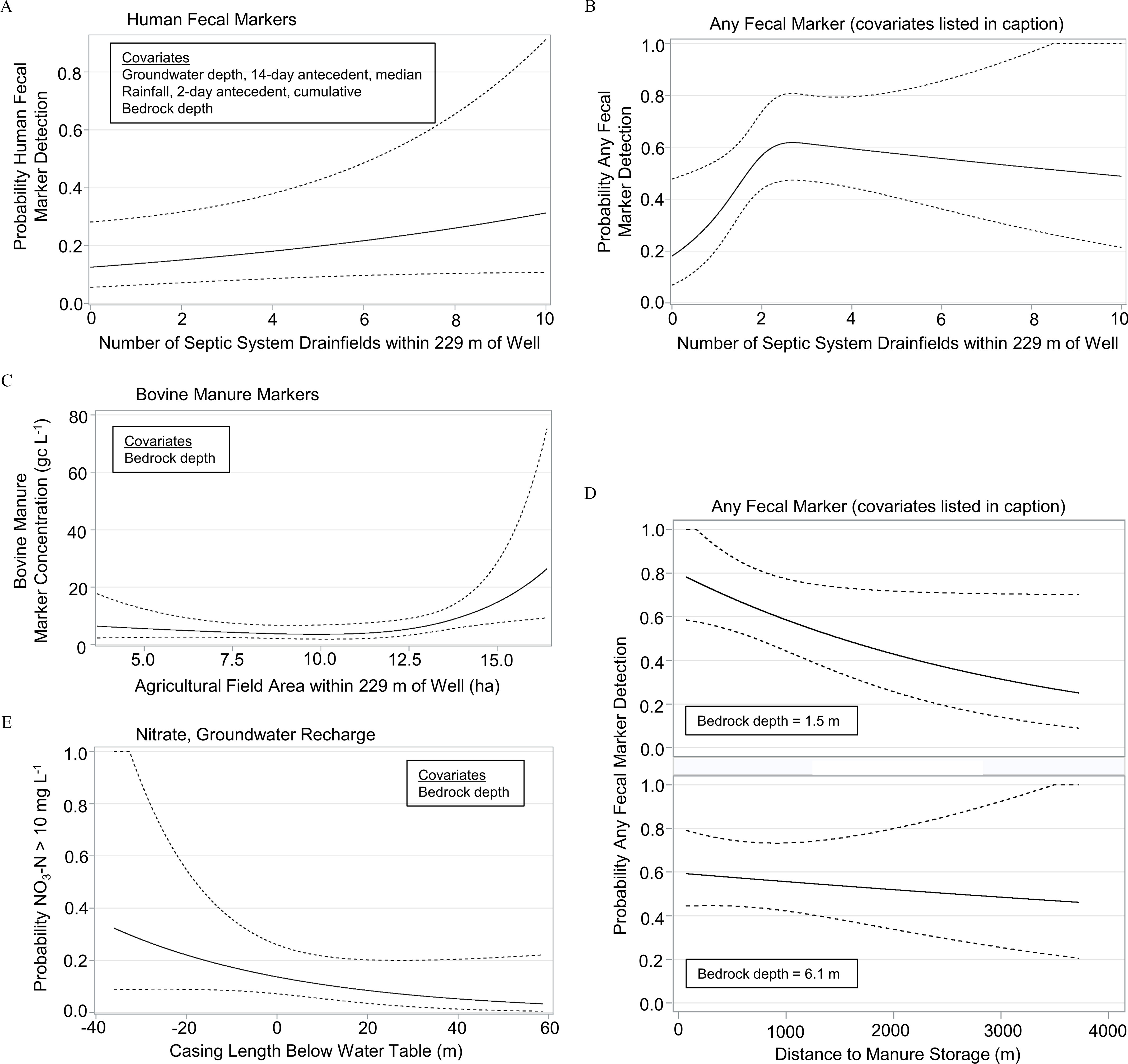
Key risk factors regressed on private well contamination probability (log-binomial regression) or concentration (gamma regression): (A) detection probability for human-specific markers; (B) detection probability for any fecal marker; covariates: manure storage distance, bedrock depth, manure storage distance times bedrock depth interaction, rainfall 2-d antecedent cumulative; (C) estimated bovine-specific marker concentration (mean sum); (D) interaction between manure storage distance and bedrock depth for any fecal marker detection probability; covariates: septic system drainfields within $229\mathrm{m}$ of well, rainfall 2-d antecedent cumulative; (E) detection probability of ${\mathrm{NO}}_3^{-}\text{-N}>10\mathrm{mg}/\mathrm{L}$. Black line: regression estimates. Dashed lines: 95% pointwise confidence limits. Coefficients and p-values are reported in Table 5. Covariates in the multivariable models were fixed at their median values for the purpose of plotting.

Considering other vulnerable aquifers, Blaschke et al. (2016) estimated the distance between septic systems and private wells needed for $12{\text{-log}}_{10}$ virus removal to achieve a risk of ${10}^{-4}$ infections/person/y, and their lower setback distance estimates for gravel and coarse gravel aquifers were $66\mathrm{m}$ and $\mathrm{1,000}\mathrm{m}$, respectively (equivalent to densities of 0.7 and 0.003 systems/ha). For limestone aquifers similar to our study site, Morrissey et al. (2015) derived a recommendation of 3.5 systems/ha from groundwater flow modeling of indicator bacteria and nitrate, and Masciopinto et al. (2008) estimated the setback required for $7{\text{-log}}_{10}$ virus reduction from municipal wastewater injected into sinkholes was $\mathrm{8,000}\mathrm{m}$. Although previous work was based on indicators and nitrate or log removal of viruses, our model is based on the probability of contamination by fecal waste specific to humans.

Risk Factors for Well Contamination with Bovine Manure Markers

The detection probability of bovine-specific markers increased during periods of groundwater recharge (Table 5), as infiltrating precipitation and snowmelt carried manure from the surface to the water table. An increase from 0 to $40\text{\hspace{0.17em}millimeters}$ cumulative recharge 7 d prior to sampling increased the detection probability of bovine markers from 13% to 50%.

Agricultural risk factors were not associated with the detection probability of bovine markers but were associated with those markers’ concentrations (see Table S10), and of these the area of agricultural fields within $229\mathrm{m}$ of wells had the strongest association. When the area exceeded 13 ha, bovine marker concentration increased (Figure 5C).

The reason we found associations between fecal sources and detection probability of human markers but not bovine markers likely stem from differences in release patterns between septic systems and manure. Septic system locations are fixed and known with certainty; the systems operate every day, continually releasing household wastewater to the subsurface. In contrast, manure applications vary in location, timing, and volume; manure could be applied near a well on one day and then not again that year. Unlike manure field applications, manure storages are like septic systems: The locations are fixed and known, meaning our distance measurements between manure storages and study wells had minimal error. This may have contributed to our finding that the “distance to manure storage” risk factor was relevant in five multivariable models.

Because manure application records were incomplete (only large farms are required to report applications), we assumed all agricultural fields near wells were potential sources of manure at the time of sampling, which was likely true for only some fields, resulting in misclassification. However, when the model was restricted to only bovine-positive samples, this restriction removed any chance of misclassification (i.e., positivity indubitably showed manure must be near the well), which likely explains why we were able to link agricultural field area to bovine marker concentration. The impact of misclassification of manured sites may have been lessened for contaminant detection models constructed with more positive samples (i.e., greater statistical power). These models (coliforms, nitrate-N, and any fecal marker) did indeed identify agricultural risk factors.

Risk Factors for Well Contamination with Markers for Any Fecal Microbe

The any fecal marker category included the 82 samples (79 wells) positive for any of the 24 microbial markers found in the fecal material of humans, bovines and ruminants, or other vertebrate hosts (Table 3). Multivariable modeling showed detection of any marker in this category was associated with well proximity to locations of both human and bovine fecal material, namely septic drainfields and manure storages. The model included two other risk factors: rainfall and bedrock depth (Table 5). Similar findings were reported by O’Dwyer et al. (2018), who showed septic system density, cattle density, rainfall, and karst bedrock in Ireland were associated with private well contamination with E. coli.

Any fecal marker detection probability increased by a factor of three when septic drainfields increased from zero to two within $229\mathrm{m}$ of wells; additional drainfields did not further increase the detection probability (Figure 5B). Manure storage distance from wells was associated with fecal contamination after accounting for its interaction with bedrock depth; for wells closer to manure storage, the probability of detecting any fecal marker increased more steeply at shallow bedrock depth (Figure 5D).

To model the concentration outcome of any fecal marker, only positive samples were included, reducing statistical power compared to the detection outcome model. Nonetheless, bedrock depth was strongly associated with fecal marker concentration after adjusting for manure storage distance and the area of agricultural fields within $229\mathrm{m}$ of wells (Table 5).

The multivariable models for any fecal marker encapsulate the key study finding: Fecal contamination in the county’s private wells stems from both septic systems and manure, and contamination is exacerbated by shallow bedrock depth and elevated rainfall. Both fecal sources release untreated wastes to the landscape at noteworthy volumes. Septic system drainfields in the county are estimated to release into the subsurface $6.79\times {10}^8\mathrm{L}$ of household wastewater per year, and the county’s cattle population produces approximately $1.74\times {10}^9\mathrm{L}$ manure (fecal and urine combined) per year (see Supplemental Material, “Septic System Effluent Volume Released Annually in Kewaunee County, Cattle Manure Volume Produced Annually in Kewaunee County”).

Precipitation as a Risk Factor for Private Well Contamination

There is ample evidence showing precipitation favors microbial contamination of private wells. Precipitation quantity in the period preceding sampling was positively associated with the occurrence in private wells of indicator bacteria (Hynds et al. 2012; O’Dwyer et al. 2014; Procopio et al. 2017; Invik 2019) human enteric viruses (Allen et al. 2017) and the human-specific Bacteroides marker HF183 (Murphy et al. 2020). The antecedent precipitation periods associated with contamination varied between 30 (Invik et al. 2019) and 5 d (Hynds et al. 2012), and even shorter periods of rainfall (24 h) may be associated with contamination of vulnerable aquifers (Morrissey et al. 2015). In our study 2-d antecedent cumulative rainfall was more strongly associated than 7- or 14-d periods with detection of any fecal marker and markers specific to humans (see Table S10). However, when rainfall was included in multivariable models it was not as strongly associated to contamination as the other risk factors (Table 5).

Well Construction Risk Factors Related to Contamination

Well construction risk factor modeling did not identify a single overriding factor. Of 14 possible multivariable models (combinations of contaminant type, recharge, and outcome measurement) only six had any variables that met the univariable screening criteria (Table 6; and see Tables S11, S12, and S13). Four of the six models involved nitrate, suggesting well construction was more related to nitrate than microbial contamination. Statistical power may have been an issue, particularly for human and bovine markers, as construction data on file with the state government were not available for 35% of study wells. Nevertheless, the quality of the well construction data was good. Our data were derived from bona fide construction records instead of relying on well-owner recall. Summary statistics for all well construction data are reported in Tables S14–S16.

Table 6.

Multivariable modeling of well construction risk factors as related to detection probabilities and concentrations of coliforms, any fecal-associated marker, and nitrate in private wells.

Contaminant and outcome measurement (n)a	Risk factor	Univariable model $p$-value	Multivariable model
			Risk factor medianb	Risk factor rangeb	Coefficient or trendc,d	$p$-valuee
Any fecal markerf detection (83)	Casing depth	0.15	17.7	12.2–48.2	Negative	0.31
	Open interval length	0.13	29.0	2.1–79.6	Positive	0.24
	Bedrock depth	0.027	4.6	0–46.6	$-0.02$	0.26
Coliforms concentration, recharge (47)	Well depth	0.047	48.8	18.3–100.6	Negative	0.59
	Casing depth	0.057	18.9	12.2–80.2	None	0.91
	Groundwater depth at construction	0.0004	12.2	1.8–36.6	Negative	0.0038
	Well age	0.0042	24	5–49	0.04	0.016
${\mathrm{NO}}_3^{-}\text{-N}>10\mathrm{mg}/\mathrm{L}$ detection, recharge (201)	Casing length below water table	0.040	8.5	–36–58.8	$-0.02$	0.13
	Bedrock depth	0.0028	6.4	0–55.2	Negative	0.28
${\mathrm{NO}}_3^{-}\text{-N}$ concentration, recharge (124)	Well age	0.15	22	2–80	Positive	0.16
	Bedrock depth	0.0063	4.7	0–31.4	Negative	0.11
${\mathrm{NO}}_3^{-}\text{-N}>10\mathrm{mg}/\mathrm{L}$ detection, no-recharge (251)	Casing depth	0.12	18.9	6.1–126.5	0.01	0.65
	Casing length below water table	0.02	8.8	–36–117.3	$-0.02$	0.33
	Bedrock depth	$<0.0001$	10.1	0.3–54.3	Negative	0.07
${\mathrm{NO}}_3^{-}\text{-N}$ concentration, no-recharge (127)	Casing depth	0.043	18.0	6.1–126.5	$-0.008$	0.57
	Casing length below water table	0.054	5.5	–19.8–117.3	Negative	0.74
	Bedrock depth	0.0019	6.7	0.3–49.4	Negative	0.0088

Note: Univariable model $p$-values used for selecting risk factors are included for reference; complete univariable statistics are provided in Tables S11, S12, and S13. Risk factor eligibility for inclusion in multivariable models is described in statistical methods.

^a$n=\text{number of samples}$ in multivariable model.

^bUnits for length and depth are meters; age is in years.

^cIn lieu of reporting multiple coefficients for spline-represented variables we report the overall trend (positive or negative).

^dInterpretation of coefficient linear terms: change in ln(detection probability) or change in ln(concentration) for a unit change in the risk factor.

^eThe composite $p$-value is reported for spline-represented variables.

^f“Any fecal marker” includes all microorganisms regardless of host specificity.

Casing depth was included in more multivariable well construction models than any other variable; minimum depths specified in well construction codes are believed to prevent contamination. However, its independent effect in the presence of other risk factors in the well construction models was equivocal; associations were weak, and trends were inconsistent (positive, negative, and none) (Table 6). Casing length below water table was the second most frequently included risk factor, and its trends were consistent; longer casing into the aquifer reduced ${\mathrm{NO}}_3^{-}\text{-N}$ contamination. For example, increasing casing length from $36\mathrm{m}$ above to $59\mathrm{m}$ below the water table decreased the probability of ${\mathrm{NO}}_3^{-}\text{-N}$ contamination $>10\mathrm{mg}/\mathrm{L}$ during recharge by 90% (Figure 5E). Placing the casing bottom deeper into the aquifer likely results in nitrate that is infiltrating from the land surface to be further diluted before it enters the well. Of 453 study wells that had data on casing length below water table, 77 wells (17%) had casings that ended above the water table, providing no dilution benefit.

Older wells tend to have greater nitrate and bacterial contamination (Yessis et al. 1996; Goss et al. 1998), but in our study, of the 14 possible multivariable models, well age was associated only with coliforms concentration during recharge (Table 6). Changes in State code in 1988 improved well construction reporting, so our construction data skewed toward newer wells (median age approximately 20 y) that comply with recent construction regulations (e.g., only one well had casing depth less than the State minimum of $12.2\mathrm{m}$.)

Well depth is frequently identified in groundwater studies as an important factor affecting nitrate and microbial contamination. Deeper wells have less nitrate (Glanville et al. 1997; Lichtenberg and Shapiro 1997; Goss et al. 1998; Allevi et al. 2013; Swistock et al. 2013; Lockhart et al. 2013; Warner and Arnold 2010), coliforms (Gonzales 2008; Goss et al. 1998; Allevi et al. 2013), E. coli (O’Dwyer et al. 2018), and human viruses (Allen et al. 2017). Warner and Arnold (2010) found that nitrate concentrations among 378 private wells in the glacial aquifer system in the United States (of which Kewaunee County is part) had less spatial and temporal variation than the variation contributed by well depth. They suggest deeper wells have older groundwater with lower dissolved oxygen favoring denitrification. Well depth was not associated with nitrate contamination in our study wells, likely because the aquifer is oxic at least to $70\mathrm{m}$ (Bradbury and Muldoon 1992).

Hynds et al. (2012) showed that well design and construction were more important than septic systems, geological setting, or precipitation in explaining the variability of thermotolerant coliform contamination in private wells in Ireland. Our findings differ. Overall, well construction was not strongly associated with nitrate and microbial contamination of private wells in the Silurian dolomite aquifer of northeastern Wisconsin. Nor are our findings unique. In a study of 180 randomly selected private wells in northeastern Ohio, well age and well depth determined from construction records were not associated with coliform contamination (Won et al. 2013). Many studies that have investigated the link between well construction and contamination included dug wells and sand points (Yessis et al. 1996; Goss et al. 1998) or wells that lacked adequate sealing between the casing and well annulus, a condition that would allow direct ingress of surface contaminants (Hynds et al. 2012; Fennell 2017). In contrast, for our study wells that have construction data, all were drilled, none were dug, and all were sealed with grout. For wells such as these, in this hydrogeological setting, it appears differences in construction have less impact on contamination than other factors.

Utility and Generalizability of Findings

We have shown private household wells open to the Silurian dolomite aquifer in Kewaunee County, Wisconsin, were contaminated with nitrate, coliform bacteria, and diverse taxa of fecal-associated microbes, some of which were pathogenic. Contamination rates depended on bedrock depth, land use, groundwater recharge, rainfall, and to a lesser extent factors related to well construction. Our examination of risk factors was comprehensive, and multivariable modeling allowed each risk factor to be evaluated for its independent effects in the presence of other factors. In addition, risk factors were analyzed as continuous-scaled variables, which aids interpretation and is amenable for policymaking, for example, establishing setback distances between private wells and agricultural fields, allowable septic system densities, or minimum bedrock depths for manure applications.

Our findings likely apply to other regions that depend on the Silurian dolomite aquifer and where agricultural and exurban land uses affect groundwater quality. The aquifer is regionally extensive and an important water supply for public, domestic, and commercial uses in six U.S. states: Wisconsin, Illinois, Iowa, Michigan, Indiana, and Ohio (USGS 2016). The Silurian dolomite aquifer in Canada extends from Lake Huron to Niagara Falls and supplies water to nearly 800,000 people in southern Ontario (Allen et al. 2017). In northeast Wisconsin the aquifer is emblematic of an open-access resource and the “tragedies” that can result when the resource becomes degraded by competing interests. Understanding how the aquifer is contaminated—the sources, extent, and factors involved—may contribute to the broader appreciation that this essential resource is shared among all who depend on it.

References

- Alhajjar BJ, Stramer SL, Cliver DO, Harkin JM. 1988. Transport modelling of biological tracers from septic systems. Water Res 22(7):907–915, 10.1016/0043-1354(88)90028-0. [DOI] [Google Scholar]
- Allen AS, Borchardt MA, Kieke BA Jr., Dunfield KE, Parker BL. 2017. Virus occurrence in private and public wells in a fractured dolostone aquifer in Canada. Hydrogeol J 25(4):1117–1136, 10.1007/s10040-017-1557-5. [DOI] [Google Scholar]
- Allevi RP, Krometis L-AH, Hagedorn C, Benham B, Lawrence AH, Ling EJ, et al. 2013. Quantitative analysis of microbial contamination in private drinking water supply systems. J Water Health 11(2):244–255, PMID: 23708572, 10.2166/wh.2013.152. [DOI] [PubMed] [Google Scholar]
- American Public Health Association. 1995. Standard Methods for the Examination of Water and Wastewater, 19th ed. Washington, DC: American Public Health Association. [Google Scholar]
- Atherholt TB, Korn LR, Louis JB, Procopio NA. 2015. Repeat sampling and coliform bacteria detection rates in New Jersey domestic wells. Groundwater Monit R 35(2):70–80. 10.1111/j.1745-6584.2012.00997.x, . [DOI] [Google Scholar]
- Bay Lake Regional Planning Commission. 2016. Kewaunee County 20-Year Comprehensive Plan Update. http://media.baylakerpc.org/media/51229/kewaunee%20county%20comp%20plan_farm%20preservation%20plan%20full%20document-%2001182017.pdf [accessed 10 September 2019].
- Beller M, Ellis A, Lee SH, Drebot MA, Jenkerson SA, Funk E, et al. 1997. Outbreak of viral gastroenteritis due to a contaminated well, international consequences. JAMA 278(7):563–568, PMID: 9268277. [PubMed] [Google Scholar]
- Bernhard AE, Field KG. 2000. Identification of nonpoint sources of fecal pollution in coastal waters by using host-specific 16S ribosomal DNA genetic markers from fecal anaerobes. Appl Environ Microbiol 66(4):1587–1594, PMID: 10742246, 10.1128/AEM.66.4.1587-1594.2000. [DOI] [PMC free article] [PubMed] [Google Scholar]
- Blaschke AP, Derx J, Zessner M, Kirnbauer R, Kavka G, Strelec H, et al. 2016. Setback distances between small biological wastewater treatment systems and drinking water wells against virus contamination in alluvial aquifers. Sci Total Environ 573:278–289, PMID: 27570196, 10.1016/j.scitotenv.2016.08.075. [DOI] [PubMed] [Google Scholar]
- Blaustein RA, Pachepsky YA, Hill RL, Shelton DR. 2015. Solid manure as a source of fecal indicator microorganisms: release under simulated rainfall. Environ Sci Technol 49(13):7860–7869, PMID: 26011817, 10.1021/acs.est.5b01095. [DOI] [PubMed] [Google Scholar]
- Borchardt MA, Chyou PH, DeVries EO, Belongia EA. 2003a. Septic system density and infectious diarrhea in a defined population of children. Environ Health Perspect 111(5):742–748, PMID: 12727604, 10.1289/ehp.5914. [DOI] [PMC free article] [PubMed] [Google Scholar]
- Borchardt MA, Bertz PD, Spencer SK, Battigelli DA. 2003b. Incidence of enteric viruses in groundwater from household wells in Wisconsin. Appl Environ Microbiol 69(2):1172–1180, PMID: 12571044, 10.1128/AEM.69.2.1172-1180.2003. [DOI] [PMC free article] [PubMed] [Google Scholar]
- Borchardt MA, Bradbury KR, Alexander EC, Archer J, Braatz L, Forest B, et al. 2011. Norovirus outbreak caused by a new septic system in a dolomite aquifer. Ground Water 49(1):85–97, PMID: 20199588, 10.1111/j.1745-6584.2010.00686.x. [DOI] [PubMed] [Google Scholar]
- Borchardt MA, Muldoon MA, Hunt RJ, Bonness DE, Firnstahl AD, Kieke BA, et al. 2019. Assessing Groundwater Quality in Kewaunee County, Wisconsin and Characterizing the Timing and Variability of Enteric Pathogen Contamination Within the Dolomite Aquifer in Northeastern Wisconsin. DNR Project Number 227, Final Report. Wisconsin Geology and Natural History Survey, Open-File Report 2019-05, 2019.
- Bradbury KR, Muldoon MA. 1992. Hydrogeology and groundwater monitoring of fractured dolomite in the Upper Door Priority Watershed, Door County, Wisconsin. Wisconsin Geological and Natural History Survey Open File Report, WOFR 1992-2, https://wgnhs.wisc.edu/catalog/publication/000776/resource/wofr199202 [accessed 22 June 2019].
- Bradbury KR, Rayne TW, Muldoon MA. 2001. Field verification of capture zones for municipal wells at Sturgeon Bay, Wisconsin. Final Report to the Wisconsin Department of Natural Resources. https://wgnhs.uwex.edu/pubs/000823/ [accessed 22 June 2019].
- Bromley DW, Cernea MM. 1989. The Management of Common Property Natural Resources: Some Conceptual and Operational Fallacies (English). World Bank Discussion Papers; No. WDP 57. Washington, DC: World Bank Group, http://documents.worldbank.org/curated/en/548811468740174575/The-management-of-common-property-natural-resources-some-conceptual-and-operational-fallacies [accessed 15 March 2018]. [Google Scholar]
- Brown DG, Johnson KM, Loveland TR, Theobald DM. 2005. Rural land-use trends in the conterminous United States, 1950–2000. Ecol Appl 15(6):1851–1863, 10.1890/03-5220. [DOI] [Google Scholar]
- Center for Watershed Science and Education Wisconsin. 2018. Well Water Viewer: Private Well Data for Wisconsin. University of Wisconsin – Stevens Point. https://www.uwsp.edu/cnr-ap/watershed/Pages/WellWaterViewer.aspx [accessed 29 March 2018].
- DeFelice NB, Johnston JE, Gibson JM. 2016. Reducing emergency department visits for acute gastrointestinal illnesses in North Carolina (USA) by extending community water service. Environ Health Perspect 124(10):1583–1591, PMID: 27203131, 10.1289/EHP160. [DOI] [PMC free article] [PubMed] [Google Scholar]
- DiSimone LA. 2009. Quality of Water from Domestic Wells in Principal Aquifers of the United States, 1991-2004. U.S. Geological Survey Scientific Investigations Report 2008–5227. http://pubs.usgs.gov/sir/2008/5227 [accessed 21 November 2019].
- Diston D, Sinreich M, Zimmermann S, Baumgartner A, Felleisen R. 2015. Evaluation of molecular- and culture-dependent MST markers to detect fecal contamination and indicate viral presence in good quality groundwater. Environ Sci Technol 49(12):7142–7151, PMID: 25871525, 10.1021/acs.est.5b00515. [DOI] [PubMed] [Google Scholar]
- Eckhardt DAV, Stackelberg PE. 1995. Relation of ground-water quality to land use on Long Island, New York. Groundwater 33(6):1019–1033, 10.1111/j.1745-6584.1995.tb00047.x. [DOI] [Google Scholar]
- Erb K, Ronk E, Koundinya V, Luczaj J. 2015. Groundwater quality changes in a karst aquifer of northeastern Wisconsin, USA: reductions of brown water incidence and bacterial contamination resulting from implementation of regional task force recommendations. Resources 4(3):655–672, 10.3390/resources4030655. [DOI] [Google Scholar]
- Final Report of the Northeast Wisconsin Karst Task Force. 2007. Erb K, Steiglitz R, eds. https://cdn.shopify.com/s/files/1/0145/8808/4272/files/G3836.pdf [accessed 12 February 2020].
- Felleiter S, McDermott K, Hall G, Sheth P, Majury A. 2020. Exploring private water wells for fecal sources and evidence of pathogen presence in the context of current testing practices for potability in Ontario. Water Qual Res J Can 55(1):93–105, 10.2166/wqrj.2019.035. [DOI] [Google Scholar]
- Fennell C. 2017. The impact of domestic wastewater treatment system effluent on private water wells: an evaluation of contamination fingerprinting techniques. Thesis. University of Dublin, Trinity College, Dublin. [Google Scholar]
- Gardner KK, Vogel RM. 2005. Predicting ground water nitrate concentration from land use. Ground Water 43(3):343–352, PMID: 15882326, 10.1111/j.1745-6584.2005.0031.x. [DOI] [PubMed] [Google Scholar]
- Gardner TED, Geary P, Gordon IAN. 1997. Ecological sustainability and on-site effluent treatment systems. Australas J Environ Manag 4(2):144–156, 10.1080/14486563.1997.10648378. [DOI] [Google Scholar]
- Garson GD. 2013. Generalized Linear Models/Generalized Estimating Equations, 2013 Edition. Asheboro, NC: Statistical Associates Publishers. [Google Scholar]
- Gibson KE, Schwab KJ, Spencer SK, Borchardt MA. 2012. Measuring and mitigating inhibition during quantitative real time PCR analysis of viral nucleic acid extracts from large-volume environmental samples. Water Res 46(13):4281–4291, PMID: 22673345, 10.1016/j.watres.2012.04.030. [DOI] [PubMed] [Google Scholar]
- Glanville TD, Baker JL, Newman JK. 1997. Statistical analysis of rural well contamination and effects of well construction. Trans ASAE 40(2):363–370, 10.13031/2013.21281. [DOI] [Google Scholar]
- Gonzales TR. 2008. The effects that well depth and wellhead protection have on bacterial contamination of private water wells in the Estes Park Valley, Colorado. J Environ Health 71(5):17–23, PMID: 19115719. [PubMed] [Google Scholar]
- Goss MJ, Barry DAJ, Rudolph DL. 1998. Contamination in Ontario farmstead domestic wells and its association with agriculture: 1. Results from drinking water wells. J Contam Hydrol 32(3–4):267–293, 10.1016/S0169-7722(98)00054-0. [DOI] [Google Scholar]
- Green HC, Haugland RA, Varma M, Millen HT, Borchardt MA, Field KG, et al. 2014. Improved HF183 quantitative real-time PCR assay for characterization of human fecal pollution in ambient surface water samples. Appl Environ Microbiol 80(10):3086–3094, PMID: 24610857, 10.1128/AEM.04137-13. [DOI] [PMC free article] [PubMed] [Google Scholar]
- Hagedorn C, Mc Coy EL, Rahe TM. 1981. The potential for ground water contamination from septic effluents. J Environ Qual 10(1):1–8, 10.2134/jeq1981.00472425001000010001x. [DOI] [Google Scholar]
- Hastie TJ, Tibshirani RJ, Friedman JH. 2001. The Elements of Statistical Learning: Data Mining, Inference, and Prediction. New York: Springer-Verlag. [Google Scholar]
- Healy RW, Cook PG. 2002. Using groundwater levels to estimate recharge. Hydrogeol J 10(1):91–109, 10.1007/s10040-001-0178-0. [DOI] [Google Scholar]
- Higashimoto Y, Ihira M, Miyazaki Y, Kuboshiki A, Yoshinaga S, Hiramatsu H, et al. 2018. Monitoring shedding of five genotypes of RotaTeq vaccine viruses by genotype s-specific real-time reverse transcription-PCR assays. J Clin Microbiol 56(6):e00035-18, PMID: 29563200, 10.1128/JCM.00035-18. [DOI] [PMC free article] [PubMed] [Google Scholar]
- Hynds PD, Misstear BD, Gill LW. 2012. Development of a microbial contamination susceptibility model for private domestic groundwater sources. Water Resour Res 48:W12504, 10.1029/2012WR012492. [DOI] [Google Scholar]
- Hynds PD, Thomas MK, Pintar KDM. 2014a. Contamination of groundwater systems in the US and Canada by enteric pathogens, 1990–2013; a review and pooled-analysis. PLoS One 9(5):e93301, PMID: 24806545, 10.1371/journal.pone.0093301. [DOI] [PMC free article] [PubMed] [Google Scholar]
- Hynds P, Misstear BD, Gill LW, Murphy HM. 2014b. Groundwater source contamination mechanisms: physicochemical profile clustering, risk factor analysis and multivariate modeling. J Contam Hydrol 159:47–56, PMID: 24583518, 10.1016/j.jconhyd.2014.02.001. [DOI] [PubMed] [Google Scholar]
- Invik J, Barkema HW, Massolo A, Neumann NF, Cey E, Checkley S. 2019. Escherichia coli contamination of rural well water in Alberta, Canada is associated with soil properties, density of livestock and precipitation. Can Water Resour J 44(3):248–262, 10.1080/07011784.2019.1595157. [DOI] [Google Scholar]
- Iturriza-Gómara M, Kang G, Gray J. 2004. Rotavirus genotyping: keeping up with an evolving population of human rotaviruses. J Clin Virol 31(4):259–265, PMID: 15494266, 10.1016/j.jcv.2004.04.009. [DOI] [PubMed] [Google Scholar]
- Jiang B, Dennehy PH, Spangenberger S, Gentsch JR, Glass RI. 1995. First detection of group C rotavirus in fecal specimens of children with diarrhea in the United States. J Infect Dis 172(1):45–50, PMID: 7797945, 10.1093/infdis/172.1.45. [DOI] [PubMed] [Google Scholar]
- Katz BG, Griffin DW, McMahon PB, Harden HS, Wade E, Hicks RW, et al. 2010. Fate of effluent-borne contaminants beneath septic tank drainfields overlying a karst aquifer. J Environ Qual 39(4):1181–1195, PMID: 20830905, 10.2134/jeq2009.0244. [DOI] [PubMed] [Google Scholar]
- Knobeloch L, Gorski P, Christenson M, Anderson H. 2013. Private drinking water quality in rural Wisconsin. J Environ Health 75(7):16–20, PMID: 23505770. [PubMed] [Google Scholar]
- Krolik J, Evans G, Belanger P, Maier A, Hall G, Joyce A, et al. 2014. Microbial source tracking and spatial analysis of E. coli contaminated private well waters in southeastern Ontario. J Water Health 12(2):348–356, PMID: 24937229, 10.2166/wh.2013.192. [DOI] [PubMed] [Google Scholar]
- Lambertini E, Spencer SK, Bertz PD, Loge FJ, Kieke BA, Borchardt MA. 2008. Concentration of enteroviruses, adenoviruses, and noroviruses from drinking water by use of glass wool filters. Appl Environ Microbiol 74(10):2990–2996, PMID: 18359827, 10.1128/AEM.02246-07. [DOI] [PMC free article] [PubMed] [Google Scholar]
- Li X, Atwill ER, Antaki E, Applegate O, Bergamaschi B, Bond RF, et al. 2015. Fecal indicator and pathogenic bacteria and their antibiotic resistance in alluvial groundwater of an irrigated agricultural region with dairies. J Environ Qual 44(5):1435–1447, PMID: 26436261, 10.2134/jeq2015.03.0139. [DOI] [PubMed] [Google Scholar]
- Lichtenberg E, Shapiro LK. 1997. Agriculture and nitrate concentrations in Maryland community water system wells. J Environ Qual 26(1):145–153, 10.2134/jeq1997.00472425002600010022x. [DOI] [Google Scholar]
- Lockhart KM, King AM, Harter T. 2013. Identifying sources of groundwater nitrate contamination in a large alluvial groundwater basin with highly diversified intensive agricultural production. J Contam Hydrol 151:140–154, PMID: 23800783, 10.1016/j.jconhyd.2013.05.008. [DOI] [PubMed] [Google Scholar]
- Lohr SL. 2010. Sampling: Design and Analysis. 2nd ed. Boston, MA: Brooks/Cole. [Google Scholar]
- Lusk MG, Toor GS, Yang Y-Y, Mechtensimer S, De M, Obreza TA. 2017. A review of the fate and transport of nitrogen, phosphorus, pathogens, and trace organic chemicals in septic systems. Crit Rev Environ Sci Technol 47(7):455–541, 10.1080/10643389.2017.1327787. [DOI] [Google Scholar]
- Madadgar O, Nazaktabar A, Keivanfar H, Zahraei Salehi T, Lotfollah Zadeh S. 2015. Genotyping and determining the distribution of prevalent G and P types of group a bovine rotaviruses between 2010 and 2012 in Iran. Vet Microbiol 179(3–4):190–196, PMID: 26072368, 10.1016/j.vetmic.2015.04.024. [DOI] [PubMed] [Google Scholar]
- Masciopinto C, La Mantia R, Chrysikopoulos CV. 2008. Fate and transport of pathogens in a fractured aquifer in the Salento area, Italy. Water Resour Res 44:W01404, 10.1029/2006WR005643. [DOI] [Google Scholar]
- Matthijnssens J, Joelsson DB, Warakomski DJ, Zhou T, Mathis PK, van Maanen MH, et al. 2010. Molecular and biological characterization of the 5 human-bovine rotavirus (WC3)-based reassortant strains of the pentavalent rotavirus vaccine, RotaTeq. Virology 403(2):111–127, PMID: 20451234, 10.1016/j.virol.2010.04.004. [DOI] [PubMed] [Google Scholar]
- McCullough DR. 1982. White-tailed deer pellet-group weights. J Wildl Manage 46(3):829–832, 10.2307/3808585. [DOI] [Google Scholar]
- McNutt LA, Wu C, Xue X, Hafner JP. 2003. Estimating the relative risk in cohort studies and clinical trials of common outcomes. Am J Epidemiol 157(10):940–943, PMID: 12746247, 10.1093/aje/kwg074. [DOI] [PubMed] [Google Scholar]
- Messier KP, Kane E, Bolich R, Serre ML. 2014. Nitrate variability in groundwater of North Carolina using monitoring and private well data models. Environ Sci Technol 48(18):10804–10812, PMID: 25148521, 10.1021/es502725f. [DOI] [PMC free article] [PubMed] [Google Scholar]
- Mieszkin S, Yala JF, Joubrel R, Gourmelon M. 2010. Phylogenetic analysis of Bacteroidales 16S rRNA gene sequences from human and animal effluents and assessment of ruminant faecal pollution by real-time PCR. J Appl Microbiol 108(3):974–984, PMID: 19735325, 10.1111/j.1365-2672.2009.04499.x. [DOI] [PubMed] [Google Scholar]
- Morrissey PJ, Johnston PM, Gill LW. 2015. The impact of on-site wastewater from high density cluster developments on groundwater quality. J Contam Hydrol 182:36–50, PMID: 26331764, 10.1016/j.jconhyd.2015.07.008. [DOI] [PubMed] [Google Scholar]
- Muldoon MA, Bradbury KR. 2010. Assessing seasonal variations in recharge and water quality in the silurian aquifer in areas with thicker soil cover. Wisconsin groundwater management practice monitoring project, DNR-198. http://digital.library.wisc.edu/1711.dl/EcoNatRes.MuldoonAssess [accessed 22 June 2019].
- Muldoon MA, Simo JA, Bradbury KR. 2001. Correlation of high-permeability zones with stratigraphy in a fractured-dolomite aquifer, Door County, Wisconsin. Hydrogeol J 9(6):570–583, 10.1007/s10040-001-0165-5. [DOI] [Google Scholar]
- Murphy HM, McGinnis S, Blunt R, Stokdyk J, Wu J, Cagle A, et al. 2020. Septic systems and rainfall influence human fecal marker and indicator organism occurrence in private wells in southeastern Pennsylvania. Environ Sci Technol 54(6):3159–3168, PMID: 32073835, 10.1021/acs.est.9b05405. [DOI] [PubMed] [Google Scholar]
- Nennich TD, Harrison JH, VanWieringen LM, Meyer D, Heinrichs AJ, Weiss WP, et al. 2005. Prediction of manure and nutrient excretion from dairy cattle. J Dairy Sci 88(10):3721–3733, PMID: 16162547, 10.3168/jds.S0022-0302(05)73058-7. [DOI] [PubMed] [Google Scholar]
- NGWA (National Groundwater Association). 2020. Groundwater Use in the United States of America. NGWA USA Groundwater Use Factsheet 01-13-2020. https://www.ngwa.org/docs/default-source/default-document-library/groundwater/usa-groundwater-use-fact-sheet.pdf?sfvrsn=5c7a0db8_4 [accessed 1July 2020].
- Nicosia LA, Rose JB, Stark L, Stewart MT. 2001. A field study of virus removal in septic tank drainfields. J Environ Qual 30(6):1933–1939, PMID: 11789999, 10.2134/jeq2001.1933. [DOI] [PubMed] [Google Scholar]
- NOAA (National Oceanic and Atmospheric Administration/National Centers for Environmental Information). n.d.. Climate at a Glance: Global Mapping. https://www.ncdc.noaa.gov/cag/ [accessed 18 March 2021].
- Nolan BT, Hitt KJ. 2006. Vulnerability of shallow groundwater and drinking-water wells to nitrate in the United States. Environ Sci Technol 40(24):7834–7840, PMID: 17256535, 10.1021/es060911u. [DOI] [PubMed] [Google Scholar]
- Nolan BT. 2001. Relating nitrogen sources and aquifer susceptibility to nitrate in shallow ground waters of the United States. Groundwater 39(2):290–299, 10.1111/j.1745-6584.2001.tb02311.x. [DOI] [PubMed] [Google Scholar]
- NRCS 313 (Natural Resources Conservation Service Conservation Practice Standard 313). Waste Storage Facility, Wisconsin Natural Resources Conservation Service, Madison, WI, January 2014.
- O’Dwyer J, Dowling A, Adley CC. 2014. Microbiological assessment of private groundwater-derived potable water supplies in the Mid-West Region of Ireland. J Water Health 12(2):310–317, PMID: 24937225, 10.2166/wh.2014.178. [DOI] [PubMed] [Google Scholar]
- O’Dwyer J, Hynds PD, Byrne KA, Ryan MP, Adley CC. 2018. Development of a hierarchical model for predicting microbiological contamination of private groundwater supplies in a geologically heterogeneous region. Environ Pollut 237:329–338, PMID: 29499576, 10.1016/j.envpol.2018.02.052. [DOI] [PubMed] [Google Scholar]
- Óhaiseadha C, Hynds PD, Fallon UB, O’Dwyer J. 2017. A geostatistical investigation of agricultural and infrastructural risk factors associated with primary verotoxigenic E. coli (VTEC) infection in the Republic of Ireland, 2008–2013. Epidemiol Infect 145(1):95–105, PMID: 27609320, 10.1017/S095026881600193X. [DOI] [PMC free article] [PubMed] [Google Scholar]
- Papp H, Laszlo B, Jakab F, Ganesh B, De Grazia S, Matthijnssens J, et al. 2013. Review of group a rotavirus strains reported in swine and cattle. Vet Microbiol 165(3–4):190–199, PMID: 23642647, 10.1016/j.vetmic.2013.03.020. [DOI] [PMC free article] [PubMed] [Google Scholar]
- Pitzer VE, Patel MM, Lopman BA, Viboud C, Parashar UD, Grenfell BT. 2011. Modeling rotavirus strain dynamics in developed countries to understand the potential impact of vaccination on genotype distributions. Proc Natl Acad Sci USA 108(48):19353–19358, PMID: 22084114, 10.1073/pnas.1110507108. [DOI] [PMC free article] [PubMed] [Google Scholar]
- Procopio NA, Atherholt TB, Goodrow SM, Lester LA. 2017. The likelihood of coliform bacteria in NJ domestic wells based on precipitation and other factors. Ground Water 55(5):722–735, PMID: 28369797, 10.1111/gwat.12518. [DOI] [PubMed] [Google Scholar]
- Rasmuson A, Erickson B, Borchardt M, Muldoon M, Johnson WP. 2020. Pathogen prevalence in fractured versus granular aquifers and the role of forward flow stagnation zones on pore-scale delivery to surfaces. Environ Sci Technol 54(1):137–145, PMID: 31770489, 10.1021/acs.est.9b03274. [DOI] [PubMed] [Google Scholar]
- Rayne TW, Bradbury KR, Krause JJ. 2019. Impacts of a rural subdivision on groundwater quality: results of long-term monitoring. Ground Water 57(2):279–291, PMID: 29603208, 10.1111/gwat.12666. [DOI] [PubMed] [Google Scholar]
- Reneau RB Jr. 1979. Changes in concentrations of selected chemical pollutants in wet, tile-drained soil systems as influenced by disposal of septic tank effluents. J Environ Qual 8(2):189–196, 10.2134/jeq1979.00472425000800020011x. [DOI] [Google Scholar]
- Riepenhoff-Talty M, Morse K, Wang CH, Shapiro C, Roberts J, Welter M, et al. 1997. Epidemiology of group C rotavirus infection in Western New York women of childbearing age. J Clin Microb 35(2):486–488, PMID: 9003623, 10.1128/JCM.35.2.486-488.1997. [DOI] [PMC free article] [PubMed] [Google Scholar]
- Schneeberger CL, O’Driscoll M, Humphrey C, Henry K, Deal N, Seiber K, et al. 2015. Fate and transport of enteric microbes from septic systems in a coastal watershed. J Environ Health 77(9):22–30, PMID: 25985535. [PubMed] [Google Scholar]
- Shaver RH, Ault CH, Ausich WI, Droste JB, Horowitz AS, James WC, et al. 1978. The Search for a Silurian Reef Model, Great Lakes Area: Indiana Department of Natural Resources Geological Survey Special Report 15. https://igws.indiana.edu/bookstore/details.cfm?Pub_Num=SR15 [accessed 29 June 2019].
- Sherrill MG. 1979. Contamination Potential in the Silurian Dolomite Aquifer, Eastern Wisconsin. USGS Water-Resources Investigations Open-File Report, 78–108. Reston, VA: USGS, 10.3133/wri78108 [accessed 1 October 2018]. [DOI] [Google Scholar]
- Sherrill MG. 1978. Geology and ground Water in Door County, Wisconsin, with Emphasis on Contamination Potential in the Silurian Dolomite. U.S. Geological Survey Water-Supply Paper 2047. Reston, VA: USGS. [Google Scholar]
- Smith CM, Hill VR. 2009. Dead-end hollow-fiber ultrafiltration for recovery of diverse microbes from water. Appl Environ Microbiol 75(16):5284–5289, PMID: 19561183, 10.1128/AEM.00456-09. [DOI] [PMC free article] [PubMed] [Google Scholar]
- Stokdyk J, Spencer SK, Walsh J, de Lambert J, Firnstahl AD, Anderson A, et al. 2019. Cryptosporidium incidence and surface water influence of groundwater supplying public water systems in Minnesota, USA. Environ Sci Technol 53(7):3391–3398, PMID: 30895775, 10.1021/acs.est.8b05446. [DOI] [PubMed] [Google Scholar]
- Stokdyk JP, Firnstahl AD, Walsh JF, Spencer SK, de Lambert JR, Anderson AC, et al. 2020. Viral, bacterial, and protozoan pathogens and fecal markers in wells supplying groundwater to public water systems in Minnesota, USA. Water Res 178:115814, PMID: 32325219, 10.1016/j.watres.2020.115814. [DOI] [PubMed] [Google Scholar]
- Strauss B, King W, Ley A, Hoey JR. 2001. A prospective study of rural drinking water quality and acute gastrointestinal illness. BMC Public Health 1:8, PMID: 11580869, 10.1186/1471-2458-1-8. [DOI] [PMC free article] [PubMed] [Google Scholar]
- Swistock BR, Clemens S, Sharpe WE, Rummel S. 2013. Water quality and management of private drinking water wells in Pennsylvania. J Environ Health 75(6):60–66, PMID: 23397651. [PubMed] [Google Scholar]
- Toetz D. 2006. Nitrate in ground and surface waters in the vicinity of a concentrated animal feeding operation. Arch Hydrobiol 166(1):67–77, 10.1127/0003-9136/2006/0166-0067. [DOI] [Google Scholar]
- Tsunemitsu H, Jiang B, Saif L. 1992. Detection of group C rotavirus antigens and antibodies in animals and humans by enzyme-linked immunosorbent assays. J Clin Microb 30(8):2129–2134, PMID: 1323577, 10.1128/JCM.30.8.2129-2134.1992. [DOI] [PMC free article] [PubMed] [Google Scholar]
- U.S. EPA. (United States Environmental Protection Agency). 1977. The Report to Congress–Waste Disposal Practices and Their Effects on Ground Water. CgD-78-120: B-166506. Washington, DC: U.S. Environmental Protection Agency. [Google Scholar]
- U.S. EPA. 2020. National Primary Drinking Water Regulations. 40 CFR Part 141 https://www.ecfr.gov/cgi-bin/text-idx?tpl=/ecfrbrowse/Title40/40cfr141_main_02.tpl [accessed 16 April 2020].
- U.S. General Accounting Office. 1997. Information on the Quality of Water Found at Community Water Systems and Private Wells. United States GAO/RCED-97-123.. Washington, DC: U.S. Government Accounting Office. [Google Scholar]
- USDA NASS (U.S. Department of Agriculture National Agricultural Statistics Service). 2002. Census of Agriculture. http://agcensus.mannlib.cornell.edu/AgCensus/getVolumeOnePart.do?year=2002&part_id=1015&number=49&title=Wisconsin [accessed 2 November 2018].
- USDA NASS. 2017. Census of Agriculture. www.nass.usda.gov/AgCensus [accessed 8 December 2020].
- USGS (U.S. Geological Survey). 2016. U.S. Geological Survey Ground Water Atlas of the United States, https://pubs.usgs.gov/ha/ha730/ Page last modified 30-Nov-2016 [accessed 27 May 2020].
- USGS (U.S. Geological Survey). 2020. USGS Water Data for the Nation: U.S. Geological Survey National Water Information System Database. 10.5066/F7P55KJN [accessed 15 September 2018]. [DOI]
- Ward MH, Jones RR, Brender JD, de Kok TM, Weyer PJ, Nolan BT, et al. 2018. Drinking water nitrate and human health: an updated review. Int J Environ Res Public Health 15(7):1557, PMID: 30041450, 10.3390/ijerph15071557. [DOI] [PMC free article] [PubMed] [Google Scholar]
- Warner KL, Arnold TL. 2010. Relations that Affect the Probability and Prediction of Nitrate Concentration in Private Wells in the Glacial Aquifer System in the United States. U.S. Geological Survey Scientific Investigations Report 2010–5100, https://pubs.usgs.gov/sir/2010/5100/ [accessed 1 April 2020].
- Wheeler DC, Nolan BT, Flory AR, DellaValle CT, Ward MH. 2015. Modeling groundwater nitrate concentrations in private wells in Iowa. Sci Total Environ 536:481–488, PMID: 26232757, 10.1016/j.scitotenv.2015.07.080. [DOI] [PMC free article] [PubMed] [Google Scholar]
- Wisconsin Department of Health Services. n.d. Drinking Water: Manure in Private Wells. https://www.dhs.wisconsin.gov/water/manure.htm [accessed 10 May 2021].
- Wisconsin Department of Natural Resources. 2018. Deer Abundance and Densities in Wisconsin Deer Management Units. https://dnr.wi.gov/topic/hunt/maps.html/falldeerperdr.pdf [accessed 12 May 2021].
- Won G, Gill A, LeJeune JT. 2013. Microbial quality and bacteria pathogens in private wells used for drinking water in northeastern Ohio. J Water Health 11(3):555–562, PMID: 23981882, 10.2166/wh.2013.247. [DOI] [PubMed] [Google Scholar]
- Yates MV. 1985. Septic tank density and ground-water contamination. Groundwater 23(5):586–591, 10.1111/j.1745-6584.1985.tb01506.x. [DOI] [Google Scholar]
- Yessis J, McColl RS, Seliske P. 1996. Methodological aspects of monitoring for microbial contamination of drinking water from private wells: the water quality program of the region of waterloo. Can Water Resour J 21(3):221–228, 10.4296/cwrj2103221. [DOI] [Google Scholar]
- Zhang Y, Kelly W, Panno SV, Liu W-T. 2014. Tracing fecal pollution sources in karst groundwater by Bacteriodales genetic biomarkers, bacterial indicators, and environmental variables. Sci Total Environ 490:1082–1090, PMID: 24922611, 10.1016/j.scitotenv.2014.05.086. [DOI] [PubMed] [Google Scholar]
- Zirkle KW, Nolan BT, Jones RR, Weyer PJ, Ward MH, Wheeler DC. 2016. Assessing the relationship between groundwater nitrate and animal feeding operations in Iowa (USA). Sci Total Environ 566-567:1062–1068, PMID: 27277210, 10.1016/j.scitotenv.2016.05.130. [DOI] [PMC free article] [PubMed] [Google Scholar]
Associated Data
This section collects any data citations, data availability statements, or supplementary materials included in this article.