Microscopic Examination of Spatial Transcriptome Using Seq-Scope

Chun-Seok Cho; Jingyue Xi; Yichen Si; Sung-Rye Park; Jer-En Hsu; Myungjin Kim; Goo Jun; Hyun Min Kang; Jun Hee Lee

doi:10.1016/j.cell.2021.05.010

. Author manuscript; available in PMC: 2022 Jun 24.

Published in final edited form as: Cell. 2021 Jun 10;184(13):3559–3572.e22. doi: 10.1016/j.cell.2021.05.010

Microscopic Examination of Spatial Transcriptome Using Seq-Scope

Chun-Seok Cho ^1,⁴, Jingyue Xi ^2,⁴, Yichen Si ², Sung-Rye Park ¹, Jer-En Hsu ¹, Myungjin Kim ¹, Goo Jun ³, Hyun Min Kang ², Jun Hee Lee ^1,^5,^*

PMCID: PMC8238917 NIHMSID: NIHMS1704034 PMID: 34115981

Summary

Spatial barcoding technologies have the potential to reveal histological details of transcriptomic profiles; however, they are currently limited by their low resolution. Here we report Seq-Scope, a spatial barcoding technology with a resolution comparable to an optical microscope. Seq-Scope is based on a solid-phase amplification of randomly barcoded single-molecule oligonucleotides using an Illumina sequencing platform. The resulting clusters annotated with spatial coordinates are processed to expose RNA-capture moiety. These RNA-capturing barcoded clusters define the pixels of Seq-Scope that are approximately 0.5-0.8 μm apart from each other. From tissue sections, Seq-Scope visualizes spatial transcriptome heterogeneity at multiple histological scales, including tissue zonation according to the portal-central (liver), crypt-surface (colon) and inflammation-fibrosis (injured liver) axes, cellular components including single cell types and subtypes, and subcellular architectures of nucleus and cytoplasm. Seq-scope is quick, straightforward, precise and easy-to-implement, and makes spatial single cell analysis accessible to a wide group of biomedical researchers.

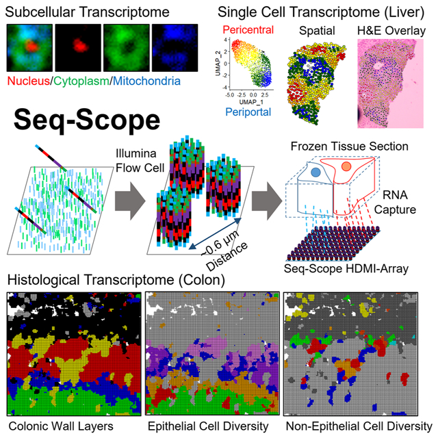
Graphical Abstract

graphic file with name nihms-1704034-f0001.jpg

In Brief:

Seq-Scope uses spatial barcoding and the Illumina sequencing platform to achieve sub-micron resolution spatial transcriptomics, enabling the visualization of transcriptomic heterogeneity at the cellular and subcellular level in various tissues.

Introduction

The development of light and electron microscopes profoundly contributed to the development of modern histology (Mazzarini et al., 2020). Protein and mRNA detection techniques, such as immunohistochemistry and RNA in situ hybridization, further allowed for examining specific biomolecules in histological slides (Callea et al., 1992). These technological advances strengthened our understanding of various pathophysiological processes and enabled the development of molecular diagnostic methods for various diseases.

Standard immunohistochemistry and RNA in situ hybridization can examine only one or a handful of target molecular species at a time; therefore, the amount of information obtained from a single experimental session is limited. To overcome this, emerging Spatial Transcriptomics (ST) techniques aim to examine all genes expressed from the genome from a single histological slide (Asp et al., 2020). There are three major methodologies to experimentally implement ST. First, the sequential in situ hybridization method, often combined with combinatorial multiplexing, can increase the number of RNA species that can be detected from a single histological section. Second, in situ sequencing can identify RNA sequences from the tissue through fluorescence-based direct sequencing. Finally, spatial barcoding methods associate RNA sequences and their spatial locations by capturing tissue RNA using a spatially-barcoded oligonucleotide array.

Among these three major methodologies, the spatial barcoding method is the most straightforward, comprehensive, widely-used, and commercially available method easily accessible by many laboratories (Asp et al., 2020). Spatial barcoding is currently achieved by microspotting (Stahl et al., 2016), barcoded bead arrays (Rodriques et al., 2019; Stickels et al., 2021; Vickovic et al., 2019), or a fabricated microfluidic channel (Liu et al., 2020). These methods, however, have an intrinsic limitation due to their low-resolution specifications. For instance, VISIUM from 10X Genomics has a center-to-center resolution of 100 μm (Bergenstrahle et al., 2020), which is worse than that of the naked eye (~40 μm). More recent technologies, such as Slide-Seq, HDST and DBiT-Seq, improved the resolution (Liu et al., 2020; Rodriques et al., 2019; Stickels et al., 2021; Vickovic et al., 2019); however, their resolutions are still far coarser than an optical microscope that has submicrometer resolution.

Here, we describe a technology for achieving submicrometer resolution spatial barcoding, designated as Seq-Scope. Our technique is based on the solid-phase amplification of a random barcode molecule, conveniently achieved by the Illumina sequencing platform (Bentley et al., 2008). Seq-Scope has a center-to-center resolution of 0.5-0.8 μm (~0.6 μm on average), far superior to previous technologies and comparable to an optical microscope. Seq-Scope also has an excellent transcriptome capture output (up to 23-27 unique molecular identifiers (UMIs)/μm² on average), which is outstanding among the available ST methodologies. When aggregated into single cell areas, the transcriptome output of Seq-Scope (~4,700 UMIs/cell on average) is even comparable to conventional single cell RNA-seq (scRNA-seq). Using Seq-Scope, we obtained transcriptome images that clearly visualize microscopic cellular and subcellular structures of the liver and colon, which were impossible to obtain through formerly existing methods.

Results

Seq-Scope Technology Overview

The Seq-Scope experiments are divided into two rounds of sequencing steps: 1^st-Seq and 2^nd-Seq (Figure 1). 1^st-Seq generates a physical array of spatially-barcoded RNA-capture molecules and a spatial map of barcodes where each barcoded sequence is associated with a spatial coordinate in the physical array. 2^nd-Seq captures mRNAs released from the tissue placed on the physical array from the 1^st-Seq, and sequences the captured molecules containing both cDNA and spatial barcode information.

1^st-Seq of Seq-Scope starts with the solid-phase amplification of a single-stranded synthetic oligonucleotide library using an Illumina sequencing platform (MiSeq in the current study; Figure 1A). The oligonucleotide “seed" molecule contains the PCR/read adapter sequences, the restriction enzyme-cleavable RNA-capture domain (oligo-dT), and the high-definition map coordinate identifier (HDMI), a spatial barcode composed of a 20-32 random nucleotide sequence. The library is amplified on a lawn surface coated with PCR adapters (Figure 1B), generating a number of clusters, each of which is derived from a single “seed” molecule. Each cluster has thousands of oligonucleotides that are identical clones of the initial oligonucleotide “seed” (Bentley et al., 2008) (Figure 1B). The HDMI sequence and spatial coordinate of each cluster are determined through a sequencing-by-synthesis (SBS) procedure using the Real-Time Analysis (RTA) software, without requiring any in-house custom image analysis (Figure 1C and S1A). After SBS, the oligonucleotides in each cluster are processed to expose the nucleotide-capture domain (Figure 1D and S1A), producing an HDMI-encoded RNA-capturing array (HDMI-array; Figure 1E), the physical array produced by 1^st-Seq of Seq-Scope.

2^nd-Seq of Seq-Scope begins with overlaying the tissue slice onto the HDMI-array (Figure 1E). The mRNAs from the tissue are used as a template to generate cDNA footprints on the HDMI-barcoded RNA capture molecule (Figure 1F and S1B). Then, the secondary strand is synthesized on the cDNA footprint using an adapter-tagged random primer (Figure 1G and S1B). Since each cDNA footprint is paired with a single random primer after washing, the random priming sequence is used as a UMI (Figure S1B). The secondary strand, which is a chimeric molecule of HDMI and cDNA sequences, is then collected and prepared as a library through PCR (Figure 1H and S1B). The paired-end sequencing of this library reveals the cDNA footprint sequence, as well as its corresponding HDMI sequence (Figure 1I and S1B).

For each HDMI sequence, 1^st-Seq provides spatial coordinate information while 2^nd-Seq provides captured cDNA information. Correspondingly, the spatial gene expression matrix is constructed by combining the 1^st-Seq and 2^nd-Seq data, which is used for various analyses (Figure S1C-S1E).

HDMI-Array Captures Spatial RNA Footprint of Tissues

Through a series of titration experiments, we produced the HDMI-array with a sequenced cluster density of up to 1.5 million clusters per mm² (Figure 2A, S2A and S2B), which is sufficient to perform single cell and subcellular analysis of the spatial transcriptome (Figure 1J).

Figure 2. — (A) Representative images of HDMI clusters visualizing “A” intensity at the 1^st (upper) and 33^rd (lower) cycles of the 1^st-Seq SBS, where 33% and >97% of clusters exhibit fluorescence, respectively. Yellow squares in the left panels are magnified in the right panels.

(B) H&E staining and its corresponding Cy3-dUTP labeling fluorescence images from fragmented liver section. Dotted lines mark tissue boundaries. Box insets highlight single cell-like patterns.

(C) H&E staining and its corresponding HDMI discovery plot drawn from the analysis of 1^st-Seq and 2^nd-Seq outputs. Brighter color in the HDMI discovery plot indicates that more HDMI was found from 2^nd-Seq in the corresponding pixel area.

(D-I) Performance comparison of different ST solutions. The values were derived from each pixel (D and F-I) or gridded area (E). nUMI, number of UMI; nGene, number of gene features; SeqScope(L) and SeqScope(C), liver and colon Seq-Scope data.

See also Figure S2.

The RNA-capturing capability of the HDMI-array was first evaluated by performing a Cy3-dUTP-mediated cDNA labeling assay using a fragmented frozen liver section. The HDMI-array successfully generated a spatial cDNA footprint that preserved the overlying tissue's gross shape (Figure 2B). The labeling assay also revealed microscopic details of cDNA footprints that resemble a single cell morphology (Figure 2B, insets), which has a fluorescence texture similar to the underlying clusters (Figure 2A and S2A).

Then, we performed the complete Seq-Scope procedure on two representative gastrointestinal tissues, the liver and colon. In each 1^st-Seq experiment, the HDMI-array was produced in 1 mm-wide circular areas of the MiSeq flow cell, also known as “tiles” (Figure S2C). The tissue sections were overlaid onto the HDMI arrays, examined by H&E staining, and subjected to 2^nd-Seq. Analysis of the 1^st-Seq and 2^nd-Seq data (Figure S1C) demonstrated that the RNA footprints were discovered mostly from tissue-overlaid regions (Figure 2C, S2D and S2E), confirming that Seq-Scope can indeed capture and analyze the spatial transcriptome from the tissues.

The Seq-Scope analysis was robust against PCR and sequencing errors; >99% of all spatial assignments were estimated to be accurate, as detailed in the STAR methods (Figure S2F-S2H). The small number of transcripts discovered outside of the tissue-overlaid regions had a transcriptome profile similar to the tissue-covered area (r = 0.9833); therefore, these transcripts are likely derived from tissue debris or ambient RNAs released from the tissue.

Seq-Scope Captures Transcriptome Information with High Efficiency

Compared to previous ST solutions, Seq-Scope offers a dramatic improvement in resolution (Figure 2D) and pixel density (Figure 2E); center-to-center distances between HDMI pixels were measured to be 0.633 ± 0.140 μm (liver) and 0.630 ± 0.132 μm (colon) (mean ± SD; Figure 2D). Although each HDMI-barcoded cluster covers an extremely tiny area (<1 μm²), single HDMI pixel in tissue-covered region was able to capture 6.70 ± 5.11 (liver) and 23.4 ± 17.4 (colon) UMIs (mean ± SD; Figure 2F). The number of gene features identified per HDMI pixel was 5.88 ± 4.22 (liver) and 19.7 ± 14.3 (colon) (mean ± SD; Figure 2G). Per-pixel counts of UMIs and genes in Seq-Scope were larger than HDST but were smaller than other technologies (Figure 2F and 2G). However, after normalization using the pixel density, Seq-Scope showed the best transcriptome capture performance per area among the datasets we examined (Figure 2H and 2I; colon dataset). Considering that the current data are estimated to cover only ~60% (liver) and ~36% (colon) of the total library size (Figure S2I), the maximum possible Seq-Scope capture efficiency should be even higher than the currently presented data. Therefore, Seq-Scope provides an outstanding mRNA capture output, in addition to providing an unmatched spatial resolution output.

Seq-Scope Reveals Nuclear-Cytoplasmic Transcriptome Architecture from Tissue Sections

mRNA is transcribed and poly-A modified in the nucleus, and transported to the cytoplasm after splicing (Figure 3A). Several RNAs in the mouse liver, such as Malat1, Neat1 and Mlxipl, exhibit strong nuclear localization (Bahar Halpern et al., 2015). On the other hand, the cytoplasmic mitochondria contains many mitochondria-encoded RNAs (mt-RNA; Figure 3A).

We spatially plotted all spliced and unspliced transcripts discovered from Seq-Scope. Intriguingly, unspliced transcript expression was restricted in tiny circles with a diameter of ~10 μm (Figure 3B and S3A), which is about the size of hepatocellular nuclei (Baratta et al., 2009). Spliced mRNAs were relatively scarce in the unspliced area, while nuclear-targeted RNAs were more abundant in the unspliced area (Figure 3B). Mt-RNAs were mostly in the spliced area (Figure 3C and S3B). These observations were substantiated by correlation analysis of the single cell images (Figure 3D and S3C).

These results suggest that spliced and unspliced transcripts are useful to determine the nuclear-cytoplasmic structure from the Seq-scope dataset. Indeed, when overlaid with H&E staining images, the unspliced RNA-enriched region generally agreed with the nuclear position (Figure 3E; note that some hepatocytes are known to be multinucleate (Donne et al., 2020)). However, in some hepatocytes, the unspliced RNA-enriched regions were not observed (Figure 3E), which can be explained by the absence of the cell’s nucleus in the tissue slice (Figure S3D), the inadequate positioning of the nucleus for RNA capture (Figure S3E) or the intrinsic variations in the rates of transcription, splicing and nuclear export (Figure S3F).

To further test the robustness of these observations, we randomly divided all genes into three independent subsets and examined the expressions of spliced and unspliced mRNAs from each subset. All three datasets similarly visualized a nuclear-cytoplasmic structure with a strong correlation (Figure 3F and S3G).

Finally, we identified nuclear centers by using unspliced transcripts (Figure 3G). Then, we searched for genes whose transcripts were enriched within 5 μm from the nuclear centers. Consistent with previous cell fractionation and RNA in situ hybridization studies (Bahar Halpern et al., 2015) and our observations described above, Malat1, Neat1 and Mlxipl were identified as the top 3 genes enriched in the nuclear area (Figure 3H). These results demonstrate that Seq-Scope can perform subcellular transcriptome studies.

Seq-Scope Performs Spatial Single Cell Analysis of Hepatocytes

Using an image segmentation method (Sage and Unser, 2003), single hepatocellular areas were identified from the H&E image (Figure 3E and 4A). The single hepatocellular transcriptome from the segmented Seq-Scope data showed a substantial number of UMIs (4,294, median; 4,734 ± 2,480, mean ± SD) and genes (1,617, median; 1,673 ± 631.7, mean ± SD), which are comparable to the recent single hepatocyte transcriptome datasets obtained from MARS-Seq (Halpern et al., 2017) and Drop-Seq (Park et al., 2020) (Figure 4B). The transcriptome content of Seq-Scope was similar to the results from the MARS-Seq, Drop-Seq and Bulk RNA-seq analyses of the normal liver (Figure S4A-S4E).

Cell type mapping analysis of the segmented single hepatocyte dataset revealed the spatial structure of hepatocellular zonation, identifying both pericentral (PC) and periportal (PP) profiles (Figure S4F), which were found in their corresponding spatial locations (Figure S4G). PP- and PC-specific genes isolated from Seq-Scope were also found in MARS-Seq and Drop-Seq data (Figure S4H; Table S1). The top 50 PC/PP genes from Drop-Seq and MARS-Seq were sufficient to classify PC/PP cells in the Seq-Scope dataset (Figure S4I; Table S1). Therefore, Seq-Scope single cell analysis agreed with the former scRNA-seq results and revealed every single cell’s actual spatial locations.

A more detailed analysis of Seq-Scope data identified multiple transcriptome layers ordered across the portal-central zonation axis (Figure 4C, 4D and S4J). Continuous mapping, instead of discrete clustering, also visualized a similar zonation pattern (Figure S4K). Many of the cluster marker genes showed a spectrum of diverse zonation patterns between the PC and PP profiles (Figure 4E). These gene expression patterns are consistent with the previous RNA in situ hybridization (Aizarani et al., 2019; Halpern et al., 2017) and immunostaining results (Park et al., 2020). However, previous studies using original ST (Hildebrandt et al., 2021) or Slide-Seq (Rodriques et al., 2019) were not able to uncover this level of detail (Figure S4L and S4M), possibly due to the limitations in resolution (Figure 2D and 2E) and RNA capture efficiency (Figure S4N and S4O).

Seq-Scope Detects Non-Parenchymal Cell Transcriptome from Liver Section.

Although hepatocytes are the major cellular component in the liver, non-parenchymal cells (NPC) such as macrophages (Mϕ; blue), hepatic stellate cells (HSC; dark green), endothelial cells (ENDO; orange) and red blood cells (RBC; red) can be found in a small portion of the histological area (Figure 4F) (Ben-Moshe and Itzkovitz, 2019). Due to their small sizes, these cells were not easily isolated through H&E-based image segmentation assays; H&E-based segmentation assay failed to reveal the NPC transcriptome except around the portal vein area (grey clusters in Figure 4C and 4D), where RBCs and Mϕs often accumulate in large quantities (Dou et al., 2019).

Therefore, alternatively, we segmented the Seq-Scope dataset with a uniform grid consisting of 10 μm-sided squares (Figure S4P-S4S). Cell type mapping analysis of the gridded Seq-Scope dataset identified the grids that correspond to these NPC cell types (Figure 4G and S4T), based on the expression of cell type-specific markers (Figure S4T-S4V; Table S2). Although most of the histological space was occupied by the hepatocellular area (Hep_PP and Hep_PC), the small and fragmented spaces scattered throughout the section represented the NPC area (Figure 4H). The locations of the Mϕ and ENDO grids (Figure 4I, first and second panels) were consistent with the spatial location of their corresponding cell type-specific marker expression (Figure 4I, arrows in the third panel) and the histologically-identified Mϕ and sinusoid areas (Figure 4I, arrows in the fourth panel) that are located around the segmentation boundaries (Figure 4I, arrows in the fifth panel). Therefore, histology-guided cell segmentation analysis and histology-agnostic square gridding analysis complemented each other in identifying different cell types.

Seq-Scope Reveals Transcriptomic Details of Histopathology Associated with Liver Injury.

The data presented above confirm that Seq-Scope can reveal the transcriptome heterogeneity and spatial complexity of the normal liver at various scales. But could Seq-Scope also reveal the pathological details of transcriptome dysregulation in diseased liver? To address this, we utilized our recently developed mouse model of early-onset liver failure that was provoked by excessive mTORC1 signaling (Cho et al., 2019). This model (Tsc1^Δhep/Depdc5^Δhep mice or TD mice) exhibits widespread hepatocellular oxidative stress, leading to localized liver damage, inflammation and fibrotic responses (Cho et al., 2019).

We first examined the cellular components of the TD liver using the gridded Seq-Scope dataset (Figure S5A-S5D). Most cell types identified from the normal liver, such as PP/PC hepatocytes and NPCs, were also discovered from the TD liver (Figure 5A, S5E and S5F; Table S3). Nuclear, cytoplasmic and mitochondrial structures were also visualized through the spatial plotting of unspliced, spliced and mt-RNA transcripts, respectively (Figure S5G).

Figure 5. — Liver from a *Tsc1^Δhep/Depdc5^Δhep* (TD) mouse, which suffers severe liver injury and inflammation (Cho et al., 2019), was examined through Seq-Scope.

(A-C) UMAP (A) and spatial plots (C, left) visualize cell type clusters of 10 μm grids. NPCs and injury-responding populations are highlighted in darker colors, and their representative cell type specific marker genes are summarized in (B). H&E images (C, right) correspond to the boxed regions in (C, left). Yellow asterisk marks the injury area.

(D-O) Transcriptomic structure of liver histopathology around dead hepatocytes (D-G) and fibrotic lesions (H-O).

(D, H and M) Cell type mapping analysis using sliding windows with 5 μm (left) and 2 μm (right) intervals.

(E, I and N) Spatial plotting of indicated cell type-specific genes in histological coordinate plane.

(F) Schematic arrangement of Mϕ-Inflamed (green), Mϕ-Kupffer (blue), Hep_Injured (red) and other cells (grey) around dead hepatocytes (black skull with yellow asterisk).

(G, K, L and O) Confocal examination of liver sections stained with antibodies detecting cell type marker proteins. DAPI-absent areas with high auto-fluorescence (yellow asterisks) mark dead hepatocytes.

(J) Schematic arrangement of Mϕ-Inflamed (green), Mϕ-Kupffer (blue), HSC-A (red) and other cells (grey) around fibrotic lesion.

See also Figure S5 and Table S3.

Former bulk RNA-seq results showed that the TD liver upregulates oxidative stress signaling pathways (Cho et al., 2019). Consistent with this, Seq-Scope identified that the TD liver expressed elevated levels of several antioxidant genes such as Gpx3 and Sepp1. Interestingly, induction of these genes was robust in PP hepatocytes, while the upregulation was not pronounced in PC hepatocytes (Figure S5H). Therefore, the oxidative stress response of the TD liver was PP-specific.

In the TD liver, we noticed that some NPC populations, such as Mϕs and HSCs, were greatly increased and differentiated into subpopulations. Mϕs were differentiated into homeostatic and inflamed populations (Mϕ-Kupffer and Mϕ-inflamed). Mϕ-Kupffer expressed Kupffer cell-specific markers such as Clec4f, while Mϕ-Inflamed expressed pro-inflammatory markers such as Cd74 and MHC-II components (Figure 5B; Table S3). Likewise, HSCs were also differentiated into normal and activated HSCs (HSC-N and HSC-A). HSC-A exhibited elevated levels of fibrotic markers such as collagens and alpha-smooth muscle actins (Acta2). In contrast, HSC-N expressed a different set of extracellular proteins, such as Ecm1 and Dcn (Figure 5B; Table S3), which were also expressed by HSCs residing in the normal liver (Table S2).

The TD liver also exhibited emerging novel cell populations. Hepatocytes exhibiting injury responses (Hep_Injured) expressed serum amyloid proteins (Figure S5F), a marker for liver injury (Sack, 2020). Although the Hep_Injured population was observed in a minor subset of normal liver hepatocytes (black clusters in Figure 4C and 4D; Figure S4T-S4V; Table S2), it became much more prevalent in the TD liver dataset (Figure 5A and S5E; Table S3). Hepatic progenitor cells (HPC) expressed a unique set of genes such as Clu, Mmp7, Spp1 and Epcam (Figure 5B; Table S3). Among these genes, Spp1 (Strazzabosco et al., 2014) and Epcam (Dolle et al., 2015) were formerly reported to be expressed by injury-responding HPCs. Interestingly, these populations of Mϕ-Inflamed, HSC-A, Hep_Injured and HPC were concentrated around the injury and inflammation sites, identified from the H&E histology images (Figure 5C; dotted rectangles). Therefore, it is likely that these cell types have an immediate pathophysiological connection with the liver injury observed in the TD liver.

Through multiscale sliding windows analysis (see STAR methods), we generated a fine spatial map of different cell types (Figure S5I). The results indicated that dead hepatocytes (asterisks in Figure 5C-5G) were surrounded by Mϕ-Inflamed, which were subsequently surrounded by Hep_Injured (Figure 5D). In contrast, Mϕ-Kupffer was more uniformly distributed throughout the liver section (Figure 5D). These observations are consistent with the spatial plotting of cell type-specific markers (Figure 5E) and suggest the transcriptomic structure of liver injury histopathology (Figure 5F).

To independently confirm these observations through orthogonal technology, we performed immunofluorescence confocal imaging of the cell type-specific markers (Cd74, Saa1/2 and Clec4f; Figure 5B and S5J-S5O). The result revealed a similar histopathological structure (Figure 5G) – Cd74-positive cells surrounded the region where no live cells were found (yellow asterisks), and Saa1/2 marked the hepatocellular injury response around the inflamed region. The Kupffer cell marker Clec4f was not associated with the injury site and was scattered throughout the space (Figure 5G). These results support the initial observations from the Seq-Scope data (Figure 5D-5F).

TD liver also exhibits fibrotic responses. In the active fibrosis area, Mϕ-Inflamed and HSC-A were very tightly intermingled with each other (Figure 5H and 5I). In contrast, Mϕ-Kupffer did not show specific spatial interaction and could be found in both fibrotic and non-fibrotic areas (Figure 5H and 5I). These observations (Figure 5J) were again reproduced with immunofluorescence imaging; the tight co-localization between Mϕ-Inflamed and HSC-A (Figure 5K), as well as the non-specific distribution of Mϕ-Kupffer (Figure 5L), were confirmed by visualizing Cd74, Acta2 and Clec4f proteins.

In addition to HSC-A, HPCs also interacted with Mϕ-Inflamed in the Seq-Scope data (Figure 5M and 5N), consistent with their known functional interactions (Viebahn et al., 2010). The interaction between HPC and Mϕ-Inflamed was also observed in immunofluorescence imaging (Figure 5O).

These results highlight the utility of Seq-Scope in identifying cell types associated with specific histopathological structures and identifying their specific cell type markers. These results also demonstrate that Seq-Scope can reveal the microscopic structure of transcriptome phenotypes in a way similar to immunofluorescence microscopy.

Seq-Scope Visualizes Histological Layers of Colonic Wall

The colon is another gastrointestinal organ with complex tissue layers, histological zonation structure, and diverse cellular components (Levine and Haggitt, 1989). Using the colon, we examined whether Seq-Scope can examine the spatial transcriptome in a non-hepatic tissue. The colonic wall is histologically divided into the colonic mucosa and the external muscle layers (Farkas et al., 2015). The colonic mucosa consists of the epithelium and lamina propria, and the epithelium is further divided into the crypt-base, transitional and surface layers (Figure 6A). Clustering analysis of the gridded Seq-Scope dataset (Figure S6A-S6E and Table S4) revealed transcriptome phenotypes corresponding to these layers (Figure 6B) and visualized their spatial locations (Figure 6C and S6F).

Seq-Scope Identifies Individual Cellular Components from Colon Tissue

In addition to visualizing the layer structure, Seq-Scope also revealed the various colonic epithelial and non-epithelial cell types (Figure 6D-6I and S6F-S6H). In the crypt base, stem/dividing, deep crypt secretory cell (DCSC) and Paneth-like cell phenotypes (Figure 6E, 6F and S6G) were identified. The stem/dividing cells expressed higher levels of ribosomal proteins while expressing lower levels of other epithelial cell-type markers (Figure 6J; Table S4). DCSCs expressed secretory cell markers, such as Agr2, Spink4 and Oit1 (Figure 6J; Table S4), while Paneth-like cells expressed Mptx1, a recently identified marker of the Paneth cell in the small intestine (Haber et al., 2017).

Seq-Scope also identified distinct cell types at the surface of the colonic mucosa (Figure 6D-6F). The top layer of the epithelial cells expressed surface colonocyte markers, such as Aqp8 (Fischer et al., 2001), Car4 (Borenshtein et al., 2009) and Saa1 (Eckhardt et al., 2010) (Figure 6J; Table S4). Some of the epithelial cells expressed goblet cell-specific markers, such as Zg16, Fcgbp and Tff3 (Haber et al., 2017; Pelaseyed et al., 2014) (Figure 6J; Table S4). In addition, Seq-Scope also identified enteroendocrine cells (EEC) expressing hormones, such as glucagon, peptide YY, insulin-like peptide and CCK (Figure 6J; Table S4).

Below the epithelium, there are connective tissue layers, including the lamina propria, submucosa, and external muscle layers. Seq-Scope identified many non-epithelial cell types from these layers, including smooth muscle, fibroblasts, enteric neurons, Mϕs and B-cells (Figure 6G-6I). These results indicate that Seq-Scope can transcriptomically recognize most of the major cell types present in the normal colonic wall.

Seq-Scope Performs Microscopic Analysis of Colonic Spatial Transcriptome

To take advantage of Seq-Scope’s high-resolution data, we employed multiscale sliding windows analysis (Figure 7A-7C) and spatial plotting of cluster markers (Figure 7D-7F; Figure S7), focusing on the same region of the colonic wall. Multiscale sliding windows analysis drew a clear line between different cellular compartments (Figure 7A-7C); the original gridding analysis (10 μm) or analysis with smaller grids (5 μm) did not reveal this level of high-resolution detail (Figure S6I-S6N). The sliding windows cluster assignments (Figure 7A-7C) were congruent with the spatial plotting of the relevant cluster marker genes (Figure 7D-7F) and H&E histology data (Figure 7G). For instance, in all of these data, B cells and Mϕs were confined to the lamina propria, while crypt base cell markers were confined to the epithelium (separated by dotted lines in Figure 7D-7G). The B cells and Mϕs are often in very close proximity (Figure 7C and 7F), likely due to their functional interactions (Spencer and Sollid, 2016). Genes specifically expressed in S and G2/M cell cycle phases (Nestorowa et al., 2016) were highly expressed in the crypt base area where stem/dividing cells are located (Levine and Haggitt, 1989); however, their expression was lower in the surface area (Figure 7H).

Discussion

The data presented here demonstrate that Seq-Scope can visualize the histological organization of the transcriptome architecture at multiple scales, including at the tissue zonation level, cellular component level and even subcellular level. Equipped with an ultra-high-resolution output and an outstanding transcriptome capture output, Seq-Scope drew a clear boundary between different tissue zones, cell types and subcellular components. Previously existing technologies could not provide this level of clarity due to their low-resolution output and/or inefficiency in transcriptome capture.

Several factors could have contributed to Seq-Scope’s high transcriptome capture efficiency. First, the dense and tight arrangement of barcoded clusters in Seq-Scope could have increased the transcriptome capture rate since they almost eliminated “blind spot” areas between the spatial features. Second, unlike some methods that produce a bumpy array surface, Seq-Scope produces a flat array surface, enabling direct interaction between the capture probe and tissue sample. Third, solid-phase amplification, limited by molecular crowding (Mercier and Slater, 2005), might have provided the two-dimensional concentration of RNA-capture probes ideal for the molecular interaction with tissue-derived RNA. Finally, biochemical strategies specific to our protocol, such as the secondary strand synthesis, retrieval, and amplification methods, could have increased the yield of transcriptome recovery.

Another benefit of Seq-Scope is its scalability and adaptability. In the current study, we used the MiSeq platform for the HDMI-array generation; however, virtually any sequencing platforms that use spatially localized amplification, such as Illumina GAIIx, HiSeq, NextSeq and NovaSeq, could be used for generation of the HDMI-array. Although MiSeq has small imaging areas, HiSeq2500 and NovaSeq can provide approximately 90 mm² and 800 mm² of the uninterrupted imaging area, respectively, offering a larger field of view. Newer sequencing methods, such as NextSeq and NovaSeq, are based on a patterned flow cell technology, which could provide more defined spatial information for the HDMI-encoded clusters. However, it is also possible that patterned nanowells may limit the effective RNA capture area, leading to a lower RNA capture efficiency.

In terms of the cost, the current MiSeq-based HDMI-array can be generated at approximately $150/mm². The cost could be further reduced to $11/mm² in HiSeq2500 or $2.6/mm² in NovaSeq, based on current costs of sequencing. As for turnaround time, the HDMI-array generation takes a day after 1^st-Seq, and library preparation can be completed in two days. A single MiSeq machine can finish 1^st-Seq in ~3 hrs since it only involves cluster generation and 25bp single-end sequencing steps. An experienced researcher can disassemble the 1^st-Seq flow cell within 5-10 min. The procedure is straightforward and not laborious or technically demanding. Therefore, Seq-Scope can make the ultra-high-resolution ST accessible for any type and scale of basic science and clinical work.

Convenience in the data analysis pipeline is another strength of Seq-Scope. Most of the Seq-Scope analyses were seamlessly performed with widely-used standard software tools, such as Illumina RTA (Ravi et al., 2018), STARsolo (Dobin et al., 2013) and Seurat (Butler et al., 2018). Being relatively effortless in an analytic perspective will be a hugely attractive factor for many experimental biologists.

However, it is worth noting that the MiSeq flow cell was not originally designed for ST (Ravi et al., 2018); therefore, exposing the cluster surface was initially challenging. In the liver dataset, scratch-associated data losses were often observed due to the damages during disassembly. When generating the colon dataset, we minimized the damage by protecting the HDMI-array with hydrogel filling. Therefore, the colon result was almost scratch-free and revealed higher numbers of UMI per area than the liver result. In the future, designing a detachable flow cell for 1^st-Seq could make this process even more straightforward.

The current HDMI-array is not encoded by the UMI sequence; therefore, we used random priming positions during the secondary strand synthesis as the alternative UMI. Based on our library size diversity (400-850bp), the UMI diversity available for a single gene is estimated to be ~400. In each HDMI, the ratios between the gene and UMI numbers are very close to 1:1 (Figure S2J), indicating that the current UMI diversity (~400) is far from saturation and should be more than enough to reliably de-duplicate sequencing reads without the risk of over-collapsing.

Nevertheless, UMI-encoded HDMI-array could be useful in the future. We experimented on generating the UMI-encoded HDMI-array by a template-based extension (Figure S1F) and found that both UMIs, produced by either random priming or array encoding, perform well in collapsing the PCR-multiplicated read sequences (Figure S1G).

Due to the extremely high number of HDMI and relatively low number of UMI per HDMI, HDMI-UMI information needs to be aggregated in some way to produce an interpretable result. In the ST field, the 10 μm feature size is considered a sweet spot for spatial single cell analysis (Marx, 2021). Consistent with this idea, data binning with 10 μm grids performed well for identifying various cell types from the liver and colon datasets, while smaller grids did not perform well. To overcome this limitation and fully utilize Seq-Scope’s high resolution, we employed three independent approaches: (1) Histology-guided image segmentation assay for spatial single cell analysis, (2) Multiscale sliding windows analysis for high-resolution cell type mapping, and (3) Direct spatial plotting to monitor spatial gene expression at high resolution. The results from these analyses demonstrated the utility of Seq-Scope in performing high-resolution spatial single cell/subcellular analysis and identifying biological information that former technologies were unable to approach.

Our results also indicate that Seq-Scope has the potential to improve and complement current scRNA-seq approaches. scRNA-seq for solid tissues requires extensive tissue dissociation and single cell sorting procedures. These procedures create very harsh conditions, which may eliminate labile cell populations and induce stress responses. Several cell types, such as elongated myofibers, lipid-laden adipocytes, and cells tightly joined by the extracellular matrix and tight junctions, are not amendable for conventional scRNA-seq. By capturing the transcriptome directly from a frozen tissue slice, Seq-Scope can capture single cell transcriptome signatures from cell types that have previously been difficult to work with.

In sum, here we report on Seq-Scope technology, which provides a versatile solution for spatial single cell and subcellular analyses. A single run of Seq-Scope could produce the microscopic gene expression imaging data for the whole transcriptome. The vast amount of information produced by Seq-Scope would accelerate scientific discoveries and might lead to a new paradigm in molecular diagnosis.

Limitations of the Study

The current Seq-Scope study focused exclusively on the poly-A-tagged transcriptome and did not uncover information beyond that. This limitation can be overcome through further research. For example, oligonucleotide- or transposase-tagged antibody cocktails were recently utilized in VISIUM (Vickovic et al., 2020) and DBiT-Seq (Deng et al., 2021; Liu et al., 2020) to spatially profile multiple protein expression or chromatin regulation. In the future, these methods could be combined with Seq-Scope to enable the microscopic characterizations of proteome or epigenome regulation in tissue sections.

STAR Methods

RESOURCE AVAILABILITY

Lead Contact

Further information and requests for resources and reagents may be directed to the corresponding author Jun Hee Lee (leeju@umich.edu).

Materials Availability

All materials used for Seq-Scope are commercially available.

Data and Code Availability

The Seq-Scope liver and colon datasets generated from this study are available at the Gene Expression Omnibus database (GEO accession no. GSE169706) as raw sequences and initial digital gene expression matrix. Processed RDS files for cell type mapping analyses and H&E histology images are available at Deep Blue Data (https://doi.org/10.7302/cjfe-wa35). Codes for the data analysis are available at Github (https://github.com/leeju-umich/Cho_Xi_Seqscope). Video Demonstration of Key Procedures is available at Youtube (https://www.youtube.com/playlist?list=PLRwwF9JZ_f5P7wXjgt90o52Jz9JyMYWf4.

EXPERIMENTAL MODEL AND SUBJECT DETAILS

Animal Tissue Samples

The liver and colon samples are described in our recent studies (Cho et al., 2019; Ro et al., 2016). The livers were collected from 8 week-old control (Depdc5^F/F/Tsc1^F/F, male) and TD (Alb-Cre/Depdc5^F/F/Tsc1^F/F, female) mice (Cho et al., 2019). The colons are from 8-week-old C57BL/6 wild-type male mice.

METHOD DETAILS

Generation of Seed HDMI-oligo Library

Seq-Scope is initiated with the generation of a HDMI-oligo seed library (Figure 1A and S1A). In the current report, we used two versions of the library – HDMI-DraI and HDMI32-DraI, whose sequences are provided below. The libraries have the same backbone structure with different lengths of HDMI sequences. HDMI is a sequence of random nucleotides designed to avoid the DraI digestion sites using Cutfree software (Storm and Jensen, 2018). HDMI32-DraI is an improved version of HDMI-DraI. For the liver and colon studies, HDMI-DraI was used. HDMI-DraI was generated by IDT as Ultramer oligonucleotides, while HDMI32-DraI was generated by Eurofins as Extremer oligonucleotides.

Backbone:

(P5 sequence) (TR1: TruSeq Read 1) (HDMI) (HR1: HDMI Read 1) (Oligo-dT) (DraI) (DraI-adapter) (P7 sequence)

HDMI-DraI:

CAAGCAGAAGACGGCATACGAGAT TCTTTCCCTACACGACGCTCTTCCGATCT NNVNNVNNVNNVNNVNNNNN TCTTGTGACTACAGCACCCTCGACTCTCGC TTTTTTTTTTTTTTTTTTTTTTTTTTT TTTAAA GACTTTCACCAGTCCATGAT GTGTAGATCTCGGTGGTCGCCGTATCATT

HDMI32-DraI:

CAAGCAGAAGACGGCATACGAGAT TCTTTCCCTACACGACGCTCTTCCGATCT NNVNBVNNVNNVNNVNNVNNVNNVNNVNNNNN TCTTGTGACTACAGCACCCTCGACTCTCGC TTTTTTTTTTTTTTTTTTTTTTTTTTT TTTAAA GACTTTCACCAGTCCATGAT GTGTAGATCTCGGTGGTCGCCGTATCATT

HDMI-oligo Cluster Generation and Sequencing through MiSeq (1^st-Seq)

HDMI-DraI or HDMI32-DraI was used as the ssDNA library and was sequenced in MiSeq using Read1-DraI as the custom Read1 primer. The Read1-DraI sequence is provided below.

Read1-DraI:

ATCATGGACTGGTGAAAGTC TTTAAA AAAAAAAAAAAAAAAAAAAAAAAAAAA GCGAGAGTCGAGGGTGCTGTAGTCACAAGA

Read1-DraI has a reverse complementary sequence covering HR1, Oligo-dT, DraI and DraI-adapter sequences of HDMI-DraI and HDMI32-DraI libraries.

Initially, the libraries were sequenced using the MiSeq v2 nano platform to titrate the ssDNA library concentration to generate the largest possible number of confidently-sequenced HDMI clusters (Figure S2A and S2B). After several rounds of optimization, HDMI-DraI was loaded at 100pM while HDMI32-DraI was loaded at 60-80pM. For actual implementation of Seq-Scope, the MiSeq v3 regular platform was used. MiSeq was performed in manual mode: 25bp single end reading (for HDMI-DraI) or 37bp single end reading (for HDMI32-DraI). The MiSeq runs were completed right after the first read without denaturation, indexing or re-synthesis steps. The flow cell was retrieved right after the completion of the single end reading steps. The MiSeq result was provided as a FASTQ file that has the HDMI sequence followed by the 5-base adapter sequence in TR1. Thumbnail images of clusters, visualized using Illumina Sequencing Analysis Viewer, were used to inspect the cluster morphology and density (Figure 2A, S2A and S2B).

The HDMI sequences contain 20-32 random nucleotides, which can produce 260 billion (20-mer in HDMI-DraI) or 1 quintillion (32-mer in HDMI32-DraI) different sequences. Due to this extreme diversity, the duplication rate of the HDMI sequence was extremely low (Figure S2G; less than 0.1% of total HDMI sequencing results), even though the MiSeq identified more than 30 million HDMI clusters. HDMI32-DraI or longer HDMI molecules, producing more diversity, could be more appropriate for future analysis involving a larger field of view.

MiSeq has 38 rectangular imaging areas, which are called “tiles”. 19 tiles are on the top of the flow cell, while the other 19 tiles are on the bottom of the flow cell (Figure S2C; tiles 2101-2119). For each sequencing output, the tile number and XY coordinates of the cluster from which the sequence originates can be found in the FASTQ output file of MiSeq. Only the bottom tiles were used for Seq-Scope analysis because the top tiles were destroyed during the flow cell disassembly.

Processing MiSeq Flow Cell into the HDMI-array

After 1^st-Seq, the MiSeq flow cell was further processed to convert HDMI-containing clusters to HDMI-array (Figure 1D). The flow cell retrieved from the MiSeq run was washed with nuclease-free water 3 times. Then, the flow cell was treated with DraI enzyme cocktail (1U DraI enzyme (#R0129, NEB) in 1X CutSmart buffer) in 37 °C overnight to completely cut out the P5 sequence and expose oligo-dT. The flow cell was then loaded with exonuclease I cocktail (1U Exo I enzyme (#M2903, NEB) in 1X Exo I buffer) in 37 °C for 45 min to eliminate non-specific ssDNA. P7-bound HDMI-DraI oligonucleotides make a duplex with Read1-DraI, so they were protected from Exo I digestion. Then, the flow cell was washed with water 3 times, 0.1N NaOH 3 times (each with 5 min incubation at room temperature, to denature and eliminate the Read1-DraI primer), 0.1M Tris (pH7.5, to neutralize the flow cell channel) 3 times (each with a brief wash), and then water 3 times (each with a brief wash).

HDMI-array Disassembly

Then, the flow cell was disassembled so that the HDMI-array was exposed to the outside and could be attached to the tissue sections. To protect the HDMI-array, agarose hydrogel (BP160, Fisher) was used to fill the flow cell channel before disassembly (for the colon dataset). 1.5% agarose suspension was prepared in water and incubated at 95 °C for 1 min. The resulting 1.5% melted agarose solution was loaded into the flow cell and chilled to solidify the gel. Using the Tungsten Carbide Tip Scriber (IMT-8806, IMT), all the boundary lines of the channel (corresponding to the imaging area) were scored. Additional lines inside of the boundaries were scored to help break the glass into small pieces. Then, the pressure was applied around the scored lines to break the glass out. Then, the glass particles and agarose debris were removed by washing with water. The top-exposed flow cell (HDMI-array; Figure S2K, left) was then ready for tissue attachment. The disassembly process could be practiced with used MiSeq flow cells, which could be obtained as a byproduct of conventional sequencing. After the practice flow cell was disassembled, the quality of cluster arrays could be inspected by staining with DNA dye, such as SYBR Gold. An exemplary SYBR Gold staining image of the disassembled flow cell with minimal array damage was provided as a reference (Figure S2K, right). It is critical to avoid scratches that damage the HDMI cluster array.

Tissue Sectioning, Attachment and Fixation

OCT-mounted fresh frozen tissue was sectioned in a cryostat (Leica CM3050S, −20 C) at a 5° cutting angle and 10 μm thickness. The tissues were maneuvered onto the HDMI-array from the cutting stage (Figure 1E). The tissue-HDMI-array sandwich was moved to room temperature, and the tissues were fixed in 4% formaldehyde (100 μl in PBS, diluted from the EM-grade 16% paraformaldehyde (#15170, Electron Microscopy Sciences)) for 10 min.

Tissue Imaging and mRNA release

The tissues were incubated 2 min in 100 μl isopropanol, and then stained with 80 μl hematoxylin (S3309, Agilent) for 5 min. After washing with water, the tissues were treated with 80 μl bluing buffer (CS702, Agilent) for 2 min. After washing with water, the tissues were treated with buffered eosin (1:9 = eosin (HT110216, Sigma): 0.45M Tris-Acetic buffer (pH 6.0)). After washing with water, the tissues were dried and mounted in 85% glycerol. The tissues were then imaged under a light microscope (MT6300, Meiji Techno). To release RNAs from the fixed tissues, the tissues were treated with 0.2 U/μL collagenase I (17018-029, Thermo Fisher) at 37 °C 20 min, and then with 1mg/mL pepsin (P7000, Sigma) in 0.1M HCl at 37 °C for 10 min, as previously described (Salmen et al., 2018).

Reverse Transcription

The tissue was washed with 40 μl 1X RT buffer containing 8 μl Maxima 5x RT Buffer (EP0751, Thermofisher), 1 μl RNase Inhibitor (30281, Lucigen) and 31 μl water. Subsequently, reverse transcription (Figure 1F and S1B) was performed by incubating the tissue-attached HDMI-array in 40 μl RT reaction solution containing 8 μl Maxima 5x RT Buffer (EP0751, Thermofisher), 8 μl 20% Ficoll PM-400 (F4375-10G, Sigma), 4 μl 10mM dNTPs (N0477L, NEB), 1 μl RNase Inhibitor (30281, Lucigen), 2 μl Maxima H- RTase (EP0751, Thermofisher), 4 μl Actinomycin D (500ng/μl, A1410, Sigma-Aldrich) and 13 μl water. The RT reaction solution was incubated in a humidified chamber at 42 °C overnight.

Tissue Digestion

The next day, the RT solution was removed, and the tissue was submerged in the exonuclease I cocktail (1U Exo I enzyme (#M2903, NEB) in 1X Exo I buffer) and incubated at 37 °C for 45 min to eliminate DNA that did not hybridize with mRNA. Then the cocktail was removed and the tissues were submerged in 1x tissue digestion buffer (100 mM Tris pH 8.0, 100 mM NaCl, 2% SDS, 5 mM EDTA, 16 U/mL Proteinase K (P8107S, NEB). The tissues were incubated at 37 °C for 40 min.

Secondary Strand Synthesis and Purification

After the tissue digestion, the HDMI-array was washed with water 3 times, 0.1N NaOH 3 times (each with 5 min incubation at room temperature), 0.1M Tris (pH7.5) 3 times (each with a brief wash), and then water 3 times (each with a brief wash). This step eliminated all mRNA from the HDMI-array.

After the washing steps, the HDMI-array was treated with a secondary strand synthesis mix (18 μl water, 3 μl NEBuffer-2, 3 μl 100 μM Truseq Read2-conjugated Random Primer with TCA GAC GTG TGC TCT TCC GAT CTN NNN NNN NN sequence (IDT), 3 μl 10 mM dNTP mix (N0477, NEB), and 3 μl Klenow Fragment (exonuclease-deficient; M0212, NEB). The HDMI-array was incubated at 37 °C for 2 hr in a humidity-controlled chamber.

After secondary strand synthesis (Figure 1G), the HDMI-array was washed with water 3 times to remove all DNAs that were not bound to the HDMI-array, so that each HDMI molecule corresponded to each single copy of the secondary strand. Then the HDMI-array was treated with 30 μl 0.1 N NaOH for 5 min to elute the secondary strand. The elution step was duplicated to collect 60 μl (in total) of the secondary strand product. The 60 μl secondary strand product was neutralized by mixing with 30 μl 3 M potassium acetate, pH5.5.

The volume of the neutralized secondary strand product was adjusted to 100 μl by adding ~10 μl water. The solution was then subjected to AMPure XP purification (A63881, Beckman Coulter) using a 1.8X bead/sample ratio, according to the manufacturer’s instruction. The final elution was performed using 40 μl water.

Library Construction and Sequencing (2^nd-Seq)

First-round library PCR was performed using Kapa HiFi Hotstart Readymix (KK2602, KAPA Biosystems) in a 100 μl reaction volume with 40 μl secondary strand product as the template and forward (TCT TTC CCT ACA CGA CGC*T*C) and reverse (TCA GAC GTG TGC TCT TCC*G*A) primers at 2 μM. Stars (*) in the primer sequences denote the phosphorothioate bond modifications. PCR condition: 95 °C 3 min, 13-15 cycles of (95 °C 30 sec, 60 °C 1 min, 72 °C 1 min), 72 °C 2 min and 4 °C infinite. PCR products were purified using AMPure XP in a 1.2X bead/sample ratio.

Second-round library PCR (Figure 1H) was performed using Kapa HiFi Hotstart Readymix (KK2602, KAPA Biosystems) in 100 μl reaction volume with 10 μl of 2 nM first-round PCR product as a template and forward (AAT GAT ACG GCG ACC ACC GAG ATC TAC ACT CTT TCC CTA CAC GAC GCT CT*T*C) and reverse (CAA GCA GAA GAC GGC ATA CGA GAT [8-mer index sequence] GTG ACT GGA GTT CAG ACG TGT GCT CTT CC*G*A) primers at 1 μM. PCR condition: 95 °C 3 min, 8-9 cycles of (95 °C 30 sec, 60 °C 30 sec, 72 °C 30 sec), 72 °C 2 min and 4 °C infinite. PCR products were purified using agarose gel elution for all products between 400-850bp size, using the Zymoclean Gel DNA Recovery Kit (D4001, Zymo Research) according to the manufacturer’s recommendation. Then the elution products were further purified using AMPure XP in a 0.6X-0.7X bead/sample ratio. The pooled libraries were subjected to paired-end (100-150bp) sequencing in the Illumina and BGI platforms at AdmeraHealth Inc., Psomagen Inc., and Beijing Genome Institute. The HDMI discovery plot assessments indicated that all sequencing platforms worked well for analyzing Seq-Scope data.

cDNA Labeling Assay

To label cDNAs on the HDMI-array, all the steps were identically performed as described above, except that, after mRNA release, the HDMI array was subjected to cDNA labeling assay (Salmen et al., 2018) instead of library generation procedures. After mRNA release, the tissue-attached HDMI array was incubated in 40uL fluorescent reverse transcription solution containing 13 μl water, 8 μl Maxima 5x RT Buffer (EP0751, Thermofisher), 8 μl 20% Ficoll PM-400 (F4375-10G, Sigma), 0.8 μl 100mM dATP (from 0446S, NEB), 0.8 μl 100mM dTTP (from 0446S, NEB), 0.8 μl 100mM dGTP (from 0446S, NEB), 0.1 μl 100mM dCTP (from 0446S, NEB), 1.5 μl 6.45mM Cy3-dCTP (B8159, APExBIO), 1 μl RNase Inhibitor (30281, Lucigen), 4 μl Actinomycin D (500ng/μl, A1410, Sigma-Aldrich) and 2 μl Maxima H- RTase (EP0751, Thermofisher). Reverse transcription was performed at 42°C overnight.

Then, the cocktail was removed and the tissues were submerged in 1x tissue digestion buffer (100 mM Tris pH 8.0, 100 mM NaCl, 2% SDS, 5 mM EDTA, 16 U/mL Proteinase K (P8107S, NEB)). The tissues were incubated at 37 °C for 40 min. After washing the HDMI-array surface with water 3 times, it was mounted in 80% glycerol and then observed under a fluorescent microscope (Meiji).

Generation and Testing of UMI-encoded HDMI-array

UMI-encoded HDMI array was generated using the HDMI-TruEcoRI library, which is similar to the other ssDNA libraries described above, but it does not have an oligo-dT sequence (Figure S1F).

Backbone:

(P5 sequence) (TR1: TruSeq Read 1) (HDMI) (HR1B: HDMI Read 1B) (EcoRI) (EcoRI adapter) (P7 sequence)

HDMI-TruEcoRI:

CAAGCAGAAGACGGCATACGAGAT TCTTTCCCTACACGACGCTCTTCCGATCT HNNBNBNBNBNBNBNBNNNN CCCGTTCGCAACATGTCTGGCGTCATA GAATTC CGCAGTCCAG GTGTAGATCTCGGTGGTCGCCGTATCATT

For MiSeq running, Read1-EcoRI was used as the read 1 primer.

Backbone:

(EcoRI adapter) (EcoRI) (HR1B)

Read1-EcoRI:

CTGGACTGCG GAATTC TATGACGCCAGACATGTTGCGAACGGG

The library was sequenced using MiSeq v2 nano platform at 100pM concentration and generated 1.4 million sequenced HDMI clusters per mm². MiSeq was performed in manual mode, 25bp single end reading, using the Read1-EcoRI as the custom Read 1 primer. The flow cell was retrieved right after the completion of the single end reading step. Then, the MiSeq flow cell was processed to attach UMI and oligo-dT sequences to the HDMI clusters. The flow cell was washed with water 3 times and then loaded with EcoRI-HF cocktail (1U EcoRI-HF (R3101, NEB) in 1X CutSmart NEB buffer) to cut out the P5 sequence. After 37 °C overnight incubation, the flow cell was washed with water 3 times, 0.1N NaOH 3 times (each with 5 min incubation at room temperature), 0.1M Tris (pH 7.5) 3 times, and then water 3 times. The flow cell was then loaded with 1X Phusion Hot Start II High-Fidelity Mastermix (F565S) containing 5 μM of UMI-oligo (sequence provided below).

Backbone:

(oligo-dA) (UMI) C (HR1B)

UMI-Oligo:

AAAAAAAAAAAAAAAAAAAAAAAAAAAAAA NNNNNNNN C TATGACGCCAGACATGTTGCGAACGGG

The flow cell was then incubated at 95 °C for 5 min, 60 °C for 1 min and 72 °C for 5 min. Then, the flow cell was loaded with an exonuclease I cocktail (see above for composition) and incubated for 45 min at 37 °C. The flow cell was then washed with water 3 times, 0.1N NaOH 3 times (each with 5 min incubation at room temperature), 0.1M Tris (pH 7.5) 3 times, and then water 3 times. This completes the generation of the UMI-encoded HDMI-array.

Performance of the UMI-encoded HDMI-array was tested using 2 μg total RNA purified from mouse liver, using the same reverse transcription and library preparation method described above (but without the tissue slice). The library was sequenced in Illumina HiSeqX and HiSeq4000 platforms.

Immunohistochemistry.

For immunohistochemistry, frozen liver sections were fixed with 4% paraformaldehyde, blocked with 1% BSA, 0.01% Triton X-100 in DPBS, and incubated with primary antibodies detecting indicated proteins, followed by staining with Alexa fluorescence-conjugated secondary antibodies and DAPI. Immunofluorescence was detected in Nikon A1 confocal microscope.

QUANTIFICATION AND STATISTICAL ANALYSIS

Input Data

There are three experimental outputs from Seq-Scope, which will serve as input data for downstream computational analysis. (1) HDMI sequence, tile and spatial coordinate information from 1^st-Seq, (2) HDMI sequence, coupled with cDNA sequence from 2^nd-Seq, and (3) Histological image obtained from H&E staining of the tissue slice.

Tissue Boundary Estimation

To estimate the tissue boundary, the HiSeq data were joined into MiSeq data according to their HDMI sequence. As a result, for each of the HiSeq data whose HDMI was found from MiSeq, the tile number and XY coordinates were assigned. Finally, using a custom python code, an HDMI discovery plot was generated to visualize the density of HiSeq HDMI in a given XY space of each tile (Figure S1C). The density plots were manually assigned to the corresponding H&E images (Figure 2C, S2D and S2E).

Read Alignment and Generation of Digital Gene Expression Matrix

Read alignment was performed using STAR/STARsolo 2.7.5c (Dobin et al., 2013), from which the digital gene expression (DGE) matrix was generated. From MiSeq data, HDMI sequences of clusters located on the bottom tile were extracted and used as a “whitelist” for the cell (HDMI) barcode after reverse complement conversion. The first 20 (HDMI-DraI version) or 30 (HDMI32-DraI) basepairs of HiSeq data Read 1 were considered as the cell (HDMI) barcode. HDMI assignments were performed using the default error correction method implemented in STARsolo (1MM_multi). Details about the spatial barcode assignment and error correction methods are described below in separate sections.

Due to the extensive washing steps after secondary strand synthesis, it was expected that each single molecule of HDMI-cDNA hybrid would lead to one secondary strand in the library. Therefore, the first 9-mer of Read 2 sequence, which is derived from the Randomer sequence, could serve as a proxy of the unique molecular identifier (UMI). Accordingly, the first 9 basepairs of HiSeq Read 2 data were copied to Read 1 and used as the unique molecular identifier (UMI). Read 2 was trimmed at the 3’ end to remove polyA tails of length 10 or greater and was then aligned to the mouse genome (mm10) using the Genefull option with no length threshold and no cell filtering (Figure S1D). For the genes whose expression couldn’t be monitored by the Genefull option, the Gene option was used to generate the gene expression discovery plots. UMIs were deduplicated using the default error correction method implemented in STARsolo (1MM_All), in which all UMIs with 1 mismatch distance to each other are collapsed (i.e., counted once).

For saturation analysis, multiple read alignments were performed using 25%, 50% and 75% subsets of the 2^nd-Seq results. The alignment output values were plotted in a graph (Figure S2I) to generate a saturation curve in Graphpad Prism 8 (Graphpad Software, Inc.). Hyperbolic regression was used to estimate the total unique transcript number in the liver (60,292,407 to 96,899,822; 95% confidence interval) and colon (308,586,493 to 510,224,639; 95% confidence interval) Seq-Scope libraries.

Error Correction Methods for Spatial Barcodes

Although the possibility of per-base error is very low, Seq-Scope involves a multi-step processing of sequences and DNA samples, so we expect that a small but non-negligible fraction of HDMI barcodes will contain errors. For example, the probability of “perfect barcode sequencing” without any errors throughout the 1^st-Seq and 2^nd-Seq steps (see below for details) was estimated to be ~92.3%, with the remaining reads potentially leading to challenges in the correct barcode assignment. However, under stochastic assumptions of sequencing errors, we estimate only <1% will have multiple errors, and our error correction procedure is robust against occasional errors occurring only once throughout the 1^st- and 2^nd-Seq steps. In the current study, error correction and demultiplexing of HDMI barcodes were performed in STARsolo using the 2^nd-Seq result as a FASTQ input, and the 1^st-Seq result as a barcode whitelist. We used the STARsolo’s default option (1MM_multi), which implements a robust statistical error correction method similar to 10X CellRanger 2.2.0. In this method, HDMIs are allowed to have one mismatch, and the posterior probability calculation is used to choose the barcode when multiple mismatched sequences are present.

In our empirical evaluation, when we did not apply any error correction method, we observed that 13.3% (liver) and 5.1% (colon) of HDMI barcodes no longer matched between 1^st- and 2^nd-Seq. These were comparable to our expected error rate of 7.7% and suggested that the error correction method we employed substantially rescued potential false negatives. On the other hand, our error correction introduced only negligible false positives. With error correction, the total fraction of false positive HDMI matches between 1^st- and 2^nd-seq was estimated to be 0.2% (liver data) and 0.7% (colon data). Therefore, our Seq-Scope procedure, combined with a standard error correction method, is robust against producing false-positive barcode assignments and also rescues a significant number of false-negative barcodes from the dataset.

Potential Sources of PCR and Sequencing Errors in Seq-Scope Processes

In the whole Seq-Scope procedure, there are three potential sources of errors: 1^st-Seq cluster generation step, 1^st-Seq sequencing step, and 2^nd-Seq library prep and sequencing steps.

1^st-Seq cluster generation (~2.3%): Even though the HDMI barcodes are randomly generated in a single-stranded oligonucleotide library, they were amplified on the flow cell surface so that every barcode in the cluster would have the same HDMI sequence. Based on the high fidelity of DNA polymerase, errors introduced during cluster generation are expected to be minimal. To estimate the extent of replication errors during cluster generation, we used a PCR fidelity estimator (Sharifian, 2010). After 25 cycles of solid-phase isothermal amplification by Bst DNA polymerase (error rate was set as 10⁻⁴), which generates approximately 1,000 copies of HDMI (20-mer nucleotide)-containing molecules per cluster (Bentley et al., 2008), it was estimated that 97.7% of molecules will have no errors, and only 2.27% of molecules will have a single error. HDMI sequences with multiple errors will be less than 0.03%. Therefore, most of the HDMI sequences in a single cluster are expected to be error-free.

1^st-Seq sequencing step (~3%): Errors can be also introduced during the sequencing step; however, the Illumina SBS is well known to be one of the most reliable high-throughput sequencing technologies. During 1^st-Seq, clusters were robustly filtered through the algorithms offered by the Real Time Analysis (RTA). Only the clusters passing filters (PF clusters) were used for the coordinate assignment. Randomly created HDMI sequences produced high and well-balanced base diversity, which enabled high-quality sequencing at high-density library-loading conditions. Consequently, the Q30 rate (having >99.9% accuracy in base calling) was very high, at above 96% (96.89% for liver 1^st-Seq and 96.21% for colon 1^st-Seq). The Q20 rate (having >99% accuracy in base calling) was even higher than 99% (99.4% for liver 1^st-Seq and 99.2% for colon 1^st-Seq). The base composition of each sequencing position was perfectly consistent with the expected HDMI sequencing pattern (NNNNNBNNBNNBNNBNNBNN) for more than 99% of all sequenced clusters (Figure S2F; 99.08% for liver 1^st-Seq and 99.09% for colon 1^st-Seq). Based on the current Q30 and Q20 rates, we estimate the total 1^st-Seq sequencing error rates for 20-mer HDMI as ~3%.

2^nd-Seq library preparation and sequencing steps (~2.4%): A small number of barcode errors could be introduced during secondary strand synthesis, PCR-based library amplification, and 2^nd-Seq sequencing reads. Based on the nature of these procedures, we do not expect that Seq-Scope will produce substantially more errors compared to the other available ST or scRNA-seq methods. For instance, the exonuclease-deficient Klenow enzyme produces 1 error per 10,000 bases. So, the error rate of 20-base HDMI will be less than 0.2%. The KAPA HIFI enzyme we used for library amplification has an extremely low error rate (1 error per 3.6 × 10⁶ bases), so even after 21-25 total cycles of amplification, the error rate of 20-base HDMI will be again less than 0.2%. Finally, if we suppose that every HDMI was sequenced in 2^nd-Seq just at Q30 (>99.9% accuracy), there will be a 2% chance of producing an error in the sequence. Therefore, the total errors produced in the 2^nd-Seq steps were estimated to be around 2.4%.

The total rate of errors (7.7%) was estimated by adding all the possible error rates of each step: 1^st-Seq cluster generation (2.3%) + 1^st-Seq sequencing (3%) + 2^nd-Seq library prep and sequencing (2.4%). Therefore, 92.3% of the final HDMI sequences were estimated to be error-free. However, in real experiments, the actual rate of errors could vary at each step; therefore, it is expected that there will be substantial variations from this value. Most importantly, these barcode errors are unlikely to produce false positives because we use a whitelist from 1^st-Seq to assign the spatial barcode. The errors will mostly contribute to a small fraction of false negatives, which are less problematic and can be recovered through error correction (see below) and/or additional sequencing.

Estimation of False-negative and False-positive Spatial Assignments during Error Correction

To estimate the rate of mismatch errors that were corrected by our pipeline, we performed spatial HDMI assignment without an error correction method (w/o Correction). Removal of error correction (w/o Correction) decreased the total number of spatially assigned (whitelisted) unique transcripts by 13.3% (liver; L to L in Figure S2H) and 5.1 % (colon; C to C in Figure S2H). These rates will be equal to the false-negative barcode assignment rate that was rescued by the error correction. The rate of multiple errors, which the current algorithm will not correct, can be estimated to be much lower than these rates (0.3% to 3%).

False-positive spatial assignment could be more problematic and should also be avoided as much as possible. To understand the extent of potential false-positive spatial assignment, we performed a reciprocal misassignment analysis – liver 2^nd-Seq results were analyzed using the colon 1^st-Seq whitelist (L to C), which is not expected to have correctly matching HDMI. Likewise, colon 2^nd-Seq results were analyzed using the liver 1^st-Seq whitelist (C to L). For the misassignment analyses, liver and colon 2^nd-Seq results that were obtained from the separate lanes of the sequencer were selected and used to eliminate the potential interference between the two datasets. Compared to the datasets with correct assignment (set as 100%; L to L and C to C), the misassigned dataset exhibited spatial assignment rates of 0.2% (L to C) and 0.7% (C to L), both of which are almost negligible (Figure S2H). Therefore, we can estimate that the rate of false-positive spatial assignment will be below 1%.

All these analyses indicate that over 99% of Seq-Scope data are accurate in the spatial assignment.

Analysis of Spliced and Unspliced Gene Expression

To obtain separate read counts for spliced and unspliced transcripts, we used the Velocyto (La Manno et al., 2018) option in the STARsolo software (Figure S1E). All spliced or unspliced mRNA reads were plotted onto the histological coordinate plane to identify nuclear-cytoplasmic structure (see below in “Visualization of Spatial Gene Expression). To test the reproducibility of the image analysis, all genes were randomly divided into three groups, and spliced and unspliced read counts were obtained independently. Images were compared with each other to calculate Pearson’s correlation coefficients in NIH ImageJ using Just Another Colocalization Plugin (JACoP) (Bolte and Cordelieres, 2006). Nuclear-specific (Malat1, Neat1 and Mlxipl) and mitochondria-encoded (all genes whose name start with “mt-“) transcripts were also plotted and analyzed. The correlation coefficients were assembled and presented in a heat map produced by Graphpad Prism 8 (Graphpad Software Inc.).

Subcellular Transcriptome Analysis

Transcriptomic nuclear centers were identified from the unspliced RNA plot using watershed local maxima detection implemented in ImageJ (Sage and Unser, 2003). HDMI transcriptome was partitioned into 14 bins according to their μm distances from the nuclear center. Then, the genes that were most significantly enriched in the nuclear area (with 5 μm from the nuclear center) were isolated.

Image Segmentation for Single Cell Analysis

To perform cell segmentation using H&E histology images, the watershed algorithm implemented in ImageJ (Sage and Unser, 2003) was utilized. The cell segmentation results isolated the single hepatocyte areas, which are consistent with the visual inspection of the H&E images (Figure 4A). Cell boundary images and cell center coordinates were exported from ImageJ, and used to aggregate Seq-Scope data so that the transcriptome information from all HDMI pixels within each segmented area were collapsed into their corresponding cell center coordinate barcode, generating a single cell-indexed DGE matrix. The DGE matrix was used for clustering analysis as described below. Single cell segmentation data and the spatial single cell annotation data were overlaid onto the histology images or unspliced RNA plot images using Adobe Photoshop CC.

Data Binning through Square Grids

Data binning was performed by dividing the imaging space into 100 μm² (10 μm-sided) square grids and collapsing all HDMI-UMI information into one barcode per grid. Alternatively, data binning was also performed with 25 μm² (5 μm-sided) square grids. After data binning, gene types were filtered to only contain protein-coding genes, lncRNA genes, and immunoglobulin/T cell receptor genes, to contain only the first-appearing splicing isoforms, and to exclude any hypothetical gene models (genes designated as Gm-number).

Cell Type Mapping (Clustering) Analysis

The binned and processed DGE matrix was analyzed in the Seurat v4 package (Butler et al., 2018). Feature number threshold was applied to remove the grids that corresponded to the area that was not overlaid by the tissue or was extensively damaged through scratches. Data were normalized using regularized negative binomial regression implemented in Seurat’s SCTransform function. Clustering was performed using the shared nearest neighbor modularity optimization implemented in Seurat’s FindClusters function. Clusters with mixed cell types were subjected to an additional round of clustering to get separation between the different cell types, while similar cell types were grouped together. UMAP (Becht et al., 2019) manifold, also built in the Seurat package, was used to assess the clustering performance. Top markers from each cluster, identified through the FindAllMarkers function, were used to infer and annotate cell types. Then the clusters were visualized in the UMAP manifold or the histological space using DimPlot and SpatialDimPlot functions, respectively. Raw and normalized transcript abundance in each tile, cluster and spatial grid was visualized through the VlnPlot, DotPlot, FeaturePlot and SpatialFeaturePlot functions built in the Seurat package. Area-proportional Venn diagrams were made using BioVenn (Hulsen et al., 2008).

Analysis of Transcripts Discovered Outside of Tissue-Overlaid Region

Some RNAs were discovered in an area where the tissue was not overlaid. It is possible that a trace of tissue fluid or debris, as well as ambient RNAs released from the tissues, may have generated this pattern. Although the RNA discovery in these regions was scarce, the compositions of RNA discovered in tissue-overlaid (nFeature > 250 in liver dataset) and non-overlaid regions (nFeature ≤ 250 in liver dataset) were very similar to each other (r = 0.9833 in Spearman coefficients). The minor differences between these two regions could be obviously explained by the different rates of ambient RNA release/capture and the different composition of cell types in the tissue debris. Therefore, it is plausible that ambient and debris-derived RNAs generated the pattern of RNA discovery in the tissue non-overlaid region.

Multiscale Sliding Windows Analysis

Multiscale analysis was employed to fine tune the annotation using FindTransferAnchors and TransferData functions implemented in Seurat. The anchors provided by the 10 μm grid dataset were used to guide other datasets produced from the same Seq-Scope result. Compared to the 10 μm grid dataset, the 5 μm grid dataset was much noisier in UMAP (Figure S6L) and spatial (Figure S6N, center) analyses even after multiscale fine tuning. To circumvent this problem, we employed the sliding windows analysis; after the initial 10 μm grid sampling, the grid was shifted both horizontally and vertically with 5 μm, 2 μm or 1 μm intervals, producing 4, 25 and 100 times more data, respectively (see Figure S6O for a schematic illustration). Then, the original 10 μm grid dataset was used to guide these sliding windows datasets to perform high-resolution cell type annotation. Sliding windows analysis with 5 μm intervals (Figure S6N, right) performed much better when compared to the 5 μm grid datasets (Figure S6N, center), and showed the UMAP pattern (Figure S6M) whose shape is more similar to the original 10 μm grid dataset (Figure S6E). Sliding windows analyses with 5 μm intervals were used to produce left panels in Figure 5D, 5H, 5I, S5I, 7A, 7B and 7C. Sliding windows analyses with 2 μm intervals were used to produce right panels in Figure 5D, 5H, 5I and S5I, and middle panels in Figure 7A, 7B and 7C. Sliding windows analyses with 1 μm intervals were used to produce the right panels in Figure 7A, 7B and 7C.

Visualization of Spatial Gene Expression

Spatial gene expression was visualized using a custom python code. Raw digital expression data of the queried gene (or gene list) were plotted onto the coordinate plane according to their HDMI spatial index. Considering the lateral RNA diffusion distance of 1.7 ± 2 μm (mean ± SD) measured from the original ST study (Stahl et al., 2016), gene expression densities were plotted as a ~3 μm-radius circle at a transparency alpha level between 0.005 and 0.5. In spatial gene expression images with a white background, the intensity of the colored spot indicates the abundance of transcripts around the spot location. Spatial gene expression images with a black background were created for genes or gene lists of high expression values, to make it easy to adjust the linear range of gene expression density and to overlay gene expression densities of different queries with different pseudo-color encoding. The inverse image of the greyscale plot was pseudo-colored with red, blue, green or grey, and the image contrast was linearly adjusted to highlight the biologically relevant spatial features. Finally, different pseudo-colored images were overlaid together to compare the gene expression patterns in the same histological coordinate plane. Cell cycle-specific genes, such as S phase- and G2/M phase-specific gene lists (Nestorowa et al., 2016), were retrieved from the Seurat package, and their mouse homologs were identified using the biomaRt package (Durinck et al., 2009). The list of cell type markers used in spatial plots can be found in Table S5.

Benchmark Analysis

The performance of Seq-Scope in liver and colon experiments were benchmarked against publicly available datasets produced by 10X VISIUM (https://support.10xgenomics.com/spatial-gene-expression/datasets/1.1.0/V1_Human_Brain_Section_1), DBiT-Seq (GEO: GSM4096261 in GSE137986) (Liu et al., 2020), Slide-Seq (Single Cell Portal: 180819_11 in SCP354) (Rodriques et al., 2019), Slide-SeqV2 (Single Cell Portal: 190921_19 in SCP815) (Stickels et al., 2021), and HDST (GEO: GSM4067523 in GSE130682) (Vickovic et al., 2019). Liver Seq-Scope dataset was separately benchmarked against former liver datasets produced using original ST (Zenodo: 10.5281/zenodo.4399655) (Hildebrandt et al., 2021) and Slide-Seq (Single Cell Portal: 1808038_8 in SCP354) (Rodriques et al., 2019). The Seq-Scope dataset had a large area that was not covered by tissues, so we isolated the tissue-overlaid HDMI pixels and used them for the benchmark analysis. Tissue-overlaid HDMI pixels were isolated from the 10 μm grid areas that were used for the cell type mapping analysis described above. Center-to-center resolution was calculated per each pixel as the distance from the closest pixel. For the technologies that have a defined pixel area (VISIUM, DBiT-Seq and HDST), pixel density was calculated as the inverse of the pixel area. For Slide-Seq, Slide-SeqV2 and Seq-Scope, pixel density was calculated in 150 μm grids (Slide-Seq and Slide-SeqV2) and 10 μm grids (Seq-Scope) of the final dataset. Grids that contained less than 10 pixels were excluded from the analysis. nUMI corresponds to the number of unique transcripts mapped to the transcriptome, and nGene corresponds to the number of gene features discovered per each pixel. nUMI/pixel and nGene/pixel values were multiplied by the average pixel density (pixel/μm²) to obtain the area-normalized nUMI and nGene (nUMI/μm² and nGene/μm², respectively) for each pixel.

UMI Efficiency Test

Efficiencies of UMI-encoding methods for collapsing duplicate read counts were evaluated using the data produced from the “Generation and Testing of UMI-encoded HDMI-array” section. UMI encoded by the HDMI-array (UMI_Array; 49^th-57^th positions of Read 1) and UMI encoded by the Random primed position (UMI_Randomer; 1^st-9^th positions of Read 2) were identified from the 2^nd-Seq results. Uncollapsed read count, read count collapsed with UMI_Array, and read count collapsed with UMI_Randomer were calculated for all the HDMI sequences observed, and their relative abundances were presented in a line graph (Figure S1G). The result indicates that both UMI_Array and UMI_Randomer are efficient in collapsing duplicate read counts of 2^nd-Seq results.

Supplementary Material

Figure S1. Seq-Scope Workflow, Related to Figure 1

(A and B) Chemistry workflow for generating HDMI-array in 1^st-Seq (A), and using the HDMI-array for constructing library for 2^nd-Seq (B). The 2^nd-Seq library is subjected to the standard next-generation sequencing workflow in Illumina and BGI platforms.

(C-E) Bioinformatics workflow for estimating tissue boundaries (C), visualizing and analyzing spatial gene expression patterns (D), and determining nuclear and cytoplasmic areas (E).

(F) Chemistry workflow for generating UMI-encoded HDMI-array in 1^st-Seq.

(G) Evaluation of UMI-encoding methods based on either random priming (UMI_Randomer) or array encoding (UMI_Array). The number of HDMI with multiple read counts was efficiently reduced by either UMI_Randomer- or UMI_Array-based collapsing methods.

See STAR Methods for details.

NIHMS1704034-supplement-1.pdf^{(588.8KB, pdf)}

Figure S2. Seq-Scope Performance, Related to Figure 2

(A) Representative images of HDMI clusters in the HDMI-array, retrieved from the Illumina sequence analysis viewer (SAV). Each picture visualizes “A” intensity at the 21^st cycle of the 1^st-Seq SBS, where >97% of HDMI clusters exhibit fluorescence.

(B) Titration of HDMI-oligo library loading concentration for obtaining maximum number of sequenced clusters. Total (red) and sequenced (blue) cluster numbers were presented for indicated 1^st-Seq conditions. Data are presented as mean ± SEM.

(D and E) Schematic diagram visualizes the tiles which were attached to the indicated liver (D, top) or colon (E, top) tissues. On the bottom, H&E staining images and their corresponding HDMI discovery plots were presented.

(F) HDMI sequencing results from 1^st-Seq. Base incorporation rate (%) at each location of the HDMI sequences in liver (left) and colon (right) 1^st-Seq is presented in a line graph. Please note that we used standard machine mixing for making random oligonucleotides. In this method, even though A:C:G:T was dispensed at 25:25:25:25, random bases potentially have variations from the designated ratio (in our case, A>C>G>T) due to the different chemical properties of the bases. The sequence pattern of 1^st-Seq is consistent with the expected sequence (NNNNNBNNBNNBNNBNNBNN) for more than 99% of sequenced clusters.

(G) Duplication rate of HDMI (standard 25-mer) and HDMI32 (extended 32-mer) in the MiSeq platform. HDMI duplication rate was very low at around 0.05%, and all duplicates were removed from the 1^st-Seq whitelist dataset before it was used for the Seq-Scope analysis.

(H) Reciprocal misassignment analysis of HDMI spatial mapping. Liver 2^nd-Seq dataset was analyzed with Liver 1^st-Seq dataset (L to L) or Colon 1^st-Seq dataset (L to C), and Colon 2^nd-Seq dataset was analyzed with Colon 1^st-Seq dataset (C to C) or Liver 1^st-Seq dataset (C to L). Alignment was performed with default error correction algorithm of STARsolo (Default) or without any error correction implementation (w/o Correction). Liver and colon 2^nd-Seq datasets that were obtained from the separate lanes of the sequencer were selected for these analyses to eliminate the potential interference between the two datasets.

(I) Saturation analysis of liver (red) and colon (blue) Seq-Scope dataset. Hyperbolic regression was used to estimate the total unique transcript number in the liver and colon Seq-Scope libraries.

(J) The number of UMI (nUMI) per HDMI pixel (left), the number of gene features (nGene) per HDMI pixel (center), and the nUMI/nGene ratio per pixel (right) are presented in violin plot.

(K) Exterior appearance (left) and SYBR Gold staining pattern (right) of the exemplarily disassembled MiSeq flow cell.

NIHMS1704034-supplement-2.pdf^{(805KB, pdf)}

Figure S3. Seq-Scope Visualizes Nuclear/Mitochondrial/Cytoplasmic Subcellular Architecture, Related to Figure 3

(A-C and G) These figures provide additional examples of Seq-Scope output that visualizes the nuclear/mitochondrial/cytoplasmic subcellular architecture.

(A) Spatial plot of all unspliced and spliced transcripts, as well as RNA species that are known to localize to nucleus in liver tissue (Nuc-targeted; Malat1, Neat1 and Mlxipl).

(B) Spatial plot of all unspliced and spliced transcripts, as well as RNA species that are encoded by mitochondrial genome (Mt-encoded).

(C) Pearson correlations (r) between the indicated transcript intensities in the single cell area were presented as a heat map.

(G) Spatial plot of unspliced and spliced transcript in three independent subsets of genes (Gene Subset 1-3). Pearson correlations (r) between these transcript intensities were presented as a heat map. S1-3, Spliced 1-3; U1-3, Unspliced 1-3.

(D-F) Potential reasons of why some segmented hepatocellular area did not exhibit nuclear/unspliced RNA-enriched area. Section slice may not contain nucleus for the cell (D). Nuclear position in the section may not be ideal for the unspliced RNA capture (E). Transcriptionally inactive nuclei may express reduced levels of unspliced RNAs (F).

NIHMS1704034-supplement-3.pdf^{(520.4KB, pdf)}

Figure S4. Spatial Single Cell Analyses Using Seq-Scope Dataset of Normal Liver, Related to Figure 4

(A-E) Comparison of Seq-Scope transcriptome with bulk RNA-Seq and scRNA-Seq transcriptome. Individual dots represent a single gene showing expression levels in both datasets. Correlations were evaluated in the Pearson coefficients between groups.

(F-I) Single hepatocyte transcriptome analysis using Seq-Scope. (F) Segmented hepatocyte transcriptomes were clustered into periportal (PP) and pericentral (PC) populations. UMAP (upper) and heat map (lower) analyses of clusters and cluster-specific genes were shown. (G) Spatial map of PP and PC hepatocellular populations. (H) Top 50 PP- and PC-specific genes overlap between Seq-Scope and two independent scRNA-seq data. (I) Clustering, UMAP (upper) and spatial plotting (lower) analyses were performed using only the top 50 PC/PP genes from Drop-Seq (left) and MARS-Seq (right).

(J) Spatial map of different hepatocellular clusters described in Figure 4D, overlaid with H&E staining and cell segmentation images. Four tiles, 2104-2107 (left to right), were analyzed. PV, portal vein; CV, central vein.

(K) UMAP (left) and spatial plotting (right) analysis colored with continuous zonation color map (UMAP1 – UMAP2).

(L-O) Spatial expressions of individual genes were plotted onto histological coordinate planes roughly covering 0.8 mm × 1 mm area, using mouse liver ST (L) and Slide-Seq (M) datasets. These plots displayed substantially lower resolution and dynamic range with less obvious spatial details, when compared to the plots generated by Seq-Scope (Figure 4E). RNA/gene capture output per pixel (N) or area (O) were compared between liver datasets produced using ST, Slide-Seq and Seq-Scope technologies.

(P-V) Normal liver Seq-Scope dataset was analyzed by data binning with 10 μm-sided square grids. (P) Spatial density plot depicting the number of UMIs discovered across 10 μm square grids. (Q) Violin plot depicting the number of gene features (nFeature) across the 10 μm square grids. Setting a 250 cutoff isolated grid units covered by the tissue area (R), each of which contains around 700 UMIs (S). A UMAP plot visualizing all clusters (T) and a dot plot (U) and UMAP plots (V) visualizing expression of cluster-specific markers are presented.

NIHMS1704034-supplement-4.pdf^{(1.4MB, pdf)}

Figure S5. Seq-Scope Analysis of Liver Injury and Inflammation, Related to Figure 5

(A-F) TD liver Seq-Scope dataset was analyzed by data binning with 10 μm-sided square grids. (A) Spatial density plot depicting the number of UMIs discovered across 10 μm square grids. (B) Violin plot depicting the number of gene features (nFeature) across the 10 μm square grids. Setting a 250 cutoff isolated grid units covered by the tissue area (C), each of which contains around 700 UMIs (D). A UMAP plot visualizing all clusters (E) and a dot plot (F) visualizing expression of cluster-specific markers.

(G) Spatial plots of unspliced, spliced and mitochondrial transcripts visualize subcellular structures.

(H) Expression of oxidative stress-responsive genes, Gpx3 and Sepp1, was examined in normal and TD liver using spatial plotting. Hepatocyte zonation is plotted in the bottom panel as a reference. Gpx3 and Sepp1 were specifically induced in PP hepatocytes of TD liver.

(I) Multi-scale cell type mapping analysis using sliding windows with 5 μm and 2 μm intervals.

(J-O) Spatial plots visualizing expression of indicated cell type marker genes in TD liver.

NIHMS1704034-supplement-5.pdf^{(1.4MB, pdf)}

Figure S6. Seq-Scope Analysis of Colonic Spatial Transcriptome, Related to Figure 6

(A-F) Colon Seq-Scope dataset was analyzed by data binning with 10 μm-sided square grids. (A) Spatial density plot depicting the number of UMIs discovered across 10 μm square grids. (B) Violin plot depicting the number of gene features (nFeature) across the 10 μm square grids. Setting a 1,000 cutoff isolated grid units covered by the tissue area (C), each of which contains around 2,700 UMIs (D). A UMAP plot visualizing all clusters (E) and spatial plots visualizing major histological layers (F), epithelial cell diversity (G), and non-epithelial cell diversity (H) are presented.

(I-K) Colon Seq-Scope dataset was analyzed by data binning with 5 μm-sided square grids. (I) Violin plot depicting the number of gene features (nFeature) across the 5 μm square grids. Setting a 250 cutoff isolated grid units covered by the tissue area (J), each of which contains around 600 UMIs (K).

(L and M) UMAP plots constructed from 5 μm grid dataset (L) and sliding windows dataset of 10 μm grids with 5 μm intervals (M). Cell type annotation was guided through the original 10 μm grid dataset (E).

(N) Multi-scale cell type mapping combined with sliding window analysis identifies clear boundaries between different cell types with high resolution. Colon Seq-Scope dataset was analyzed using simple gridding with 10 μm-sided squares (left). Using the 10 μm dataset as an anchor, multi-scale cell type mapping was performed in 5 μm gridding dataset (center). Even though 5 μm gridding improved the resolution, the image was very noisy due to scarce genetic information in each grid. To overcome this, we performed the same analysis using a dataset produced by sliding windows analysis of 10 μm gridding dataset with 5 μm intervals. The output images (right) clearly visualize the boundaries between different cell types with high resolution. Cell type annotations depict major histological layers (upper), epithelial cell diversity (middle), and non-epithelial cell diversity (lower).

(O) Schematic diagrams depicting the sliding windows analysis methodology. Compared to the 10 μm grid dataset, 5 μm grid dataset produces higher resolution; however, the transcriptome information revealed by 5 μm grid area is only 25% of what was recovered from 10 μm grid area. Correspondingly, 5 μm dataset produced substantial noises in cell type assignment. To overcome this, sliding windows analysis was performed to maintain transcriptome information per pixel while achieving higher resolution of cell type mapping by oversampling the data 4 times (5 μm interval), 25 times (2 μm interval) or 100 times (1 μm interval; scheme not shown).

NIHMS1704034-supplement-6.pdf^{(1.2MB, pdf)}

Figure S7. Seq-Scope Visualized Spatial Expression Patterns of Different Colonic Cell Type Markers, Related to Figure 7

(A-J) Marker genes for indicated cell types were plotted onto the histological coordinate plane with indicated colors. Top row of each panel represents the combined plotting of all listed markers. Bottom rows represent gene expression plotting of individual cell type marker genes. For all spatial plots, width and height of the imaging areas are approximately 800 μm and 1 mm, respectively.

NIHMS1704034-supplement-7.pdf^{(2.1MB, pdf)}

Table S1. Top 50 periportal (PP) and pericentral (PC) hepatocyte markers isolated from MARS-Seq, Drop-Seq and Seq-Scope data, related to Figure 4

NIHMS1704034-supplement-8.csv^{(2.4KB, csv)}

Table S2. List of genes that show cluster-specific expression patterns in the Seq-Scope normal liver dataset binned with 10 μm square grids, related to Figure 4

p_val, unadjusted P value; avg_logFC, log fold-change of the average expression between the cluster and the background; pct.1, the percentage of cells where the gene is detected in the cluster; pct.2, the percentage of cells where the gene is detected in the background; p_val_adj, bonferroni-corrected p-values. For UMAP visualization, please see Figure S4T.

NIHMS1704034-supplement-9.csv^{(22.7KB, csv)}

Table S3. List of genes that show cluster-specific expression patterns in the Seq-Scope TD liver dataset binned with 10 μm square grids, related to Figure 5

NIHMS1704034-supplement-10.csv^{(45.3KB, csv)}

Table S4. List of genes that show cluster-specific expression patterns in the Seq-Scope colon dataset binned with 10 μm square grids, related to Figure 6

NIHMS1704034-supplement-11.csv^{(122.1KB, csv)}

Table S5. List of cell type markers that were used to generate spatial plots. Marker gene list used in each figure is summarized in each tab of the excel file, related to Figure 7

NIHMS1704034-supplement-12.xlsx^{(12.7KB, xlsx)}

Highlights:

Seq-Scope repurposes Illumina sequencing platform for spatial transcriptomics
Seq-Scope achieves submicrometer resolution and efficient transcriptome capture
Seq-Scope enabled spatial single cell and subcellular analysis of liver and colon

Acknowledgments

The authors thank Drs. Euisik Yoon, Hojoong Kwak, Chang H. Kim, Seungwon Jung and Yongsung Kim and Ms. Irene Hwang for their helpful advice and comments. We thank Psomagen Inc. and the U-M Microbiome Core for their help in experiments. The work was supported by the NIH (T32AG000114 to C.S.C., K01AG061236 to M.K, U01HL137182 to H.M.K., J.X. and Y.S, R01DK118631 and R03HD098552 to G.J., R01DK114131 and R01DK102850 to J.H.L., P30AG024824, P30DK034933, P30DK089503, P30CA046592, P30AR069620, and U2CDK110768), Chan Zuckerberg Initiative (to H.M.K.), Frankel Cardiovascular Center Inaugural grant (to J.H.L. and M.K.), American Association for the Study of Liver Diseases (to J.H.L. and H.M.K.), Mcubed (to M.K., H.M.K. and J.H.L.), Glenn Foundation (to J.H.L.), Taiwan Government Scholarship (to J.E.H.), and ADVANCE and MTRAC awards (to J.H.L.), funded by the Michigan Economic Development Corporation.

Footnotes

Publisher's Disclaimer: This is a PDF file of an unedited manuscript that has been accepted for publication. As a service to our customers we are providing this early version of the manuscript. The manuscript will undergo copyediting, typesetting, and review of the resulting proof before it is published in its final form. Please note that during the production process errors may be discovered which could affect the content, and all legal disclaimers that apply to the journal pertain.

Declaration of Interests

J.H.L is an inventor on pending patent applications related to Seq-Scope. H.M.K. is presently an employee of Regeneron Pharmaceuticals, in which he owns stock and stock options.

References

Aizarani N, Saviano A, Sagar, Mailly L, Durand S, Herman JS, Pessaux P, Baumert TF, and Grun D (2019). A human liver cell atlas reveals heterogeneity and epithelial progenitors. Nature 572, 199–204. [DOI] [PMC free article] [PubMed] [Google Scholar]
Asp M, Bergenstrahle J, and Lundeberg J (2020). Spatially Resolved Transcriptomes-Next Generation Tools for Tissue Exploration. Bioessays 42, e1900221. [DOI] [PubMed] [Google Scholar]
Bahar Halpern K, Caspi I, Lemze D, Levy M, Landen S, Elinav E, Ulitsky I, and Itzkovitz S (2015). Nuclear Retention of mRNA in Mammalian Tissues. Cell Rep 13, 2653–2662. [DOI] [PMC free article] [PubMed] [Google Scholar]
Baratta JL, Ngo A, Lopez B, Kasabwalla N, Longmuir KJ, and Robertson RT (2009). Cellular organization of normal mouse liver: a histological, quantitative immunocytochemical, and fine structural analysis. Histochem Cell Biol 131, 713–726. [DOI] [PMC free article] [PubMed] [Google Scholar]
Becht E, McInnes L, Healy J, Dutertre CA, Kwok IWH, Ng LG, Ginhoux F, and Newell EW (2019). Dimensionality reduction for visualizing single-cell data using UMAP. Nat Biotechnol 37, 38–44. [DOI] [PubMed] [Google Scholar]
Ben-Moshe S, and Itzkovitz S (2019). Spatial heterogeneity in the mammalian liver. Nat Rev Gastroenterol Hepatol 16, 395–410. [DOI] [PubMed] [Google Scholar]
Bentley DR, Balasubramanian S, Swerdlow HP, Smith GP, Milton J, Brown CG, Hall KP, Evers DJ, Barnes CL, Bignell HR, et al. (2008). Accurate whole human genome sequencing using reversible terminator chemistry. Nature 456, 53–59. [DOI] [PMC free article] [PubMed] [Google Scholar]
Bergenstrahle J, Larsson L, and Lundeberg J (2020). Seamless integration of image and molecular analysis for spatial transcriptomics workflows. BMC Genomics 21, 482. [DOI] [PMC free article] [PubMed] [Google Scholar]
Bolte S, and Cordelieres FP (2006). A guided tour into subcellular colocalization analysis in light microscopy. J Microsc 224, 213–232. [DOI] [PubMed] [Google Scholar]
Borenshtein D, Schlieper KA, Rickman BH, Chapman JM, Schweinfest CW, Fox JG, and Schauer DB (2009). Decreased expression of colonic Slc26a3 and carbonic anhydrase iv as a cause of fatal infectious diarrhea in mice. Infect Immun 77, 3639–3650. [DOI] [PMC free article] [PubMed] [Google Scholar]
Butler A, Hoffman P, Smibert P, Papalexi E, and Satija R (2018). Integrating single-cell transcriptomic data across different conditions, technologies, and species. Nat Biotechnol 36, 411–420. [DOI] [PMC free article] [PubMed] [Google Scholar]
Callea F, Sergi C, Medicina D, Pizzorni S, Brisigotti M, Fabbretti G, and Bonino F (1992). From immunohistochemistry to in situ hybridization. Liver 12, 290–295. [DOI] [PubMed] [Google Scholar]
Cho CS, Kowalsky AH, Namkoong S, Park SR, Wu S, Kim B, James A, Gu B, Semple IA, Tohamy MA, et al. (2019). Concurrent activation of growth factor and nutrient arms of mTORC1 induces oxidative liver injury. Cell Discov 5, 60. [DOI] [PMC free article] [PubMed] [Google Scholar]
Deng Y, Zhang D, Liu Y, Su G, Enninful A, Bai Z, and Fan R (2021). Spatial Epigenome Sequencing at Tissue Scale and Cellular Level. bioRxiv, 10.1101/2021.1103.1111.434985. [DOI] [Google Scholar]
Dobin A, Davis CA, Schlesinger F, Drenkow J, Zaleski C, Jha S, Batut P, Chaisson M, and Gingeras TR (2013). STAR: ultrafast universal RNA-seq aligner. Bioinformatics 29, 15–21. [DOI] [PMC free article] [PubMed] [Google Scholar]
Dolle L, Theise ND, Schmelzer E, Boulter L, Gires O, and van Grunsven LA (2015). EpCAM and the biology of hepatic stem/progenitor cells. Am J Physiol Gastrointest Liver Physiol 308, G233–250. [DOI] [PMC free article] [PubMed] [Google Scholar]
Donne R, Saroul-Ainama M, Cordier P, Celton-Morizur S, and Desdouets C (2020). Polyploidy in liver development, homeostasis and disease. Nat Rev Gastroenterol Hepatol 17, 391–405. [DOI] [PubMed] [Google Scholar]
Dou L, Shi X, He X, and Gao Y (2019). Macrophage Phenotype and Function in Liver Disorder. Front Immunol 10, 3112. [DOI] [PMC free article] [PubMed] [Google Scholar]
Durinck S, Spellman PT, Birney E, and Huber W (2009). Mapping identifiers for the integration of genomic datasets with the R/Bioconductor package biomaRt. Nat Protoc 4, 1184–1191. [DOI] [PMC free article] [PubMed] [Google Scholar]
Eckhardt ER, Witta J, Zhong J, Arsenescu R, Arsenescu V, Wang Y, Ghoshal S, de Beer MC, de Beer FC, and de Villiers WJ (2010). Intestinal epithelial serum amyloid A modulates bacterial growth in vitro and pro-inflammatory responses in mouse experimental colitis. BMC Gastroenterol 10, 133. [DOI] [PMC free article] [PubMed] [Google Scholar]
Farkas AE, Gerner-Smidt C, Lili L, Nusrat A, and Capaldo CT (2015). Cryosectioning Method for Microdissection of Murine Colonic Mucosa. J Vis Exp, e53112. [DOI] [PMC free article] [PubMed] [Google Scholar]
Fischer H, Stenling R, Rubio C, and Lindblom A (2001). Differential expression of aquaporin 8 in human colonic epithelial cells and colorectal tumors. BMC Physiol 1, 1. [DOI] [PMC free article] [PubMed] [Google Scholar]
Haber AL, Biton M, Rogel N, Herbst RH, Shekhar K, Smillie C, Burgin G, Delorey TM, Howitt MR, Katz Y, et al. (2017). A single-cell survey of the small intestinal epithelium. Nature 551, 333–339. [DOI] [PMC free article] [PubMed] [Google Scholar]
Halpern KB, Shenhav R, Matcovitch-Natan O, Toth B, Lemze D, Golan M, Massasa EE, Baydatch S, Landen S, Moor AE, et al. (2017). Single-cell spatial reconstruction reveals global division of labour in the mammalian liver. Nature 542, 352–356. [DOI] [PMC free article] [PubMed] [Google Scholar]
Hildebrandt F, Andersson A, Saarenpää S, Larsson L, Van Hul N, Kanatani S, Masek J, Ellis E, Barragan A, Mollbrink A, et al. (2021). Spatial Transcriptomics to define transcriptional patterns of zonation and structural components in the liver. bioRxiv. [DOI] [PMC free article] [PubMed] [Google Scholar]
Hulsen T, de Vlieg J, and Alkema W (2008). BioVenn - a web application for the comparison and visualization of biological lists using area-proportional Venn diagrams. BMC Genomics 9, 488. [DOI] [PMC free article] [PubMed] [Google Scholar]
La Manno G, Soldatov R, Zeisel A, Braun E, Hochgerner H, Petukhov V, Lidschreiber K, Kastriti ME, Lonnerberg P, Furlan A, et al. (2018). RNA velocity of single cells. Nature 560, 494–498. [DOI] [PMC free article] [PubMed] [Google Scholar]
Levine DS, and Haggitt RC (1989). Normal histology of the colon. Am J Surg Pathol 13, 966–984. [DOI] [PubMed] [Google Scholar]
Liu Y, Yang M, Deng Y, Su G, Enninful A, Guo CC, Tebaldi T, Zhang D, Kim D, Bai Z, et al. (2020). High-Spatial-Resolution Multi-Omics Sequencing via Deterministic Barcoding in Tissue. Cell 183, 1665–1681 e1618. [DOI] [PMC free article] [PubMed] [Google Scholar]
Marx V (2021). Method of the Year: spatially resolved transcriptomics. Nat Methods 18, 9–14. [DOI] [PubMed] [Google Scholar]
Mazzarini M, Falchi M, Bani D, and Migliaccio AR (2020). Evolution and new frontiers of histology in biomedical research. Microsc Res Tech 84, 217–237. [DOI] [PMC free article] [PubMed] [Google Scholar]
Mercier JF, and Slater GW (2005). Solid phase DNA amplification: a Brownian dynamics study of crowding effects. Biophys J 89, 32–42. [DOI] [PMC free article] [PubMed] [Google Scholar]
Nestorowa S, Hamey FK, Pijuan Sala B, Diamanti E, Shepherd M, Laurenti E, Wilson NK, Kent DG, and Gottgens B (2016). A single-cell resolution map of mouse hematopoietic stem and progenitor cell differentiation. Blood 128, e20–31. [DOI] [PMC free article] [PubMed] [Google Scholar]
Park SR, Cho CS, Xi J, Kang HM, and Lee JH (2020). Holistic Characterization of Single Hepatocyte Transcriptome Responses to High Fat Diet. Am J Physiol Endocrinol Metab 320, E244–E258. [DOI] [PMC free article] [PubMed] [Google Scholar]
Pelaseyed T, Bergstrom JH, Gustafsson JK, Ermund A, Birchenough GM, Schutte A, van der Post S, Svensson F, Rodriguez-Pineiro AM, Nystrom EE, et al. (2014). The mucus and mucins of the goblet cells and enterocytes provide the first defense line of the gastrointestinal tract and interact with the immune system. Immunol Rev 260, 8–20. [DOI] [PMC free article] [PubMed] [Google Scholar]
Ravi RK, Walton K, and Khosroheidari M (2018). MiSeq: A Next Generation Sequencing Platform for Genomic Analysis. Methods Mol Biol 1706, 223–232. [DOI] [PubMed] [Google Scholar]
Ro SH, Xue X, Ramakrishnan SK, Cho CS, Namkoong S, Jang I, Semple IA, Ho A, Park HW, Shah YM, et al. (2016). Tumor suppressive role of sestrin2 during colitis and colon carcinogenesis. Elife 5, 12204. [DOI] [PMC free article] [PubMed] [Google Scholar]
Rodriques SG, Stickels RR, Goeva A, Martin CA, Murray E, Vanderburg CR, Welch J, Chen LM, Chen F, and Macosko EZ (2019). Slide-seq: A scalable technology for measuring genome-wide expression at high spatial resolution. Science 363, 1463–1467. [DOI] [PMC free article] [PubMed] [Google Scholar]
Sack GH Jr. (2020). Serum Amyloid A (SAA) Proteins. Subcell Biochem 94, 421–436. [DOI] [PubMed] [Google Scholar]
Sage D, and Unser M (2003). Teaching image-processing programming in Java. IEEE Signal Processing Magazine 20, 43–52. [Google Scholar]
Salmen F, Stahl PL, Mollbrink A, Navarro JF, Vickovic S, Frisen J, and Lundeberg J (2018). Barcoded solid-phase RNA capture for Spatial Transcriptomics profiling in mammalian tissue sections. Nat Protoc 13, 2501–2534. [DOI] [PubMed] [Google Scholar]
Sharifian H (2010). Errors induced during PCR amplification. In Department of Computer Science (Swiss Federal Institute of Technology), pp. 10.3929/ethz-a-006088024. [DOI] [Google Scholar]
Spencer J, and Sollid LM (2016). The human intestinal B-cell response. Mucosal Immunol 9, 1113–1124. [DOI] [PubMed] [Google Scholar]
Stahl PL, Salmen F, Vickovic S, Lundmark A, Navarro JF, Magnusson J, Giacomello S, Asp M, Westholm JO, Huss M, et al. (2016). Visualization and analysis of gene expression in tissue sections by spatial transcriptomics. Science 353, 78–82. [DOI] [PubMed] [Google Scholar]
Stickels RR, Murray E, Kumar P, Li J, Marshall JL, Di Bella DJ, Arlotta P, Macosko EZ, and Chen F (2021). Highly sensitive spatial transcriptomics at near-cellular resolution with Slide-seqV2. Nat Biotechnol 39, 313–319. [DOI] [PMC free article] [PubMed] [Google Scholar]
Storm AJ, and Jensen PA (2018). Designing Randomized DNA Sequences Free of Restriction Enzyme Recognition Sites. Biotechnol J 13, 10.1002/biot.201700326. [DOI] [PMC free article] [PubMed] [Google Scholar]
Strazzabosco M, Fabris L, and Albano E (2014). Osteopontin: a new player in regulating hepatic ductular reaction and hepatic progenitor cell responses during chronic liver injury. Gut 63, 1693–1694. [DOI] [PMC free article] [PubMed] [Google Scholar]
Vickovic S, Eraslan G, Salmen F, Klughammer J, Stenbeck L, Schapiro D, Aijo T, Bonneau R, Bergenstrahle L, Navarro JF, et al. (2019). High-definition spatial transcriptomics for in situ tissue profiling. Nat Methods 16, 987–990. [DOI] [PMC free article] [PubMed] [Google Scholar]
Vickovic S, Lötstedt B, Klughammer J, Segerstolpe Å, Rozenblatt-Rosen O, and Regev A (2020). SM-Omics: An automated platform for high-throughput spatial multi-omics. bioRxiv, 10.1101/2020.1110.1114.338418. [DOI] [PMC free article] [PubMed] [Google Scholar]
Viebahn CS, Benseler V, Holz LE, Elsegood CL, Vo M, Bertolino P, Ganss R, and Yeoh GC (2010). Invading macrophages play a major role in the liver progenitor cell response to chronic liver injury. J Hepatol 53, 500–507. [DOI] [PubMed] [Google Scholar]

Associated Data

This section collects any data citations, data availability statements, or supplementary materials included in this article.

Supplementary Materials

Figure S1. Seq-Scope Workflow, Related to Figure 1

(C-E) Bioinformatics workflow for estimating tissue boundaries (C), visualizing and analyzing spatial gene expression patterns (D), and determining nuclear and cytoplasmic areas (E).

(F) Chemistry workflow for generating UMI-encoded HDMI-array in 1^st-Seq.

See STAR Methods for details.

NIHMS1704034-supplement-1.pdf^{(588.8KB, pdf)}

Figure S2. Seq-Scope Performance, Related to Figure 2

(I) Saturation analysis of liver (red) and colon (blue) Seq-Scope dataset. Hyperbolic regression was used to estimate the total unique transcript number in the liver and colon Seq-Scope libraries.

(J) The number of UMI (nUMI) per HDMI pixel (left), the number of gene features (nGene) per HDMI pixel (center), and the nUMI/nGene ratio per pixel (right) are presented in violin plot.

(K) Exterior appearance (left) and SYBR Gold staining pattern (right) of the exemplarily disassembled MiSeq flow cell.

NIHMS1704034-supplement-2.pdf^{(805KB, pdf)}

Figure S3. Seq-Scope Visualizes Nuclear/Mitochondrial/Cytoplasmic Subcellular Architecture, Related to Figure 3

(A-C and G) These figures provide additional examples of Seq-Scope output that visualizes the nuclear/mitochondrial/cytoplasmic subcellular architecture.

(A) Spatial plot of all unspliced and spliced transcripts, as well as RNA species that are known to localize to nucleus in liver tissue (Nuc-targeted; Malat1, Neat1 and Mlxipl).

(B) Spatial plot of all unspliced and spliced transcripts, as well as RNA species that are encoded by mitochondrial genome (Mt-encoded).

(C) Pearson correlations (r) between the indicated transcript intensities in the single cell area were presented as a heat map.

NIHMS1704034-supplement-3.pdf^{(520.4KB, pdf)}

Figure S4. Spatial Single Cell Analyses Using Seq-Scope Dataset of Normal Liver, Related to Figure 4

(K) UMAP (left) and spatial plotting (right) analysis colored with continuous zonation color map (UMAP1 – UMAP2).

NIHMS1704034-supplement-4.pdf^{(1.4MB, pdf)}

Figure S5. Seq-Scope Analysis of Liver Injury and Inflammation, Related to Figure 5

(G) Spatial plots of unspliced, spliced and mitochondrial transcripts visualize subcellular structures.

(I) Multi-scale cell type mapping analysis using sliding windows with 5 μm and 2 μm intervals.

(J-O) Spatial plots visualizing expression of indicated cell type marker genes in TD liver.

NIHMS1704034-supplement-5.pdf^{(1.4MB, pdf)}

Figure S6. Seq-Scope Analysis of Colonic Spatial Transcriptome, Related to Figure 6

NIHMS1704034-supplement-6.pdf^{(1.2MB, pdf)}

Figure S7. Seq-Scope Visualized Spatial Expression Patterns of Different Colonic Cell Type Markers, Related to Figure 7

NIHMS1704034-supplement-7.pdf^{(2.1MB, pdf)}

Table S1. Top 50 periportal (PP) and pericentral (PC) hepatocyte markers isolated from MARS-Seq, Drop-Seq and Seq-Scope data, related to Figure 4

NIHMS1704034-supplement-8.csv^{(2.4KB, csv)}

Table S2. List of genes that show cluster-specific expression patterns in the Seq-Scope normal liver dataset binned with 10 μm square grids, related to Figure 4

NIHMS1704034-supplement-9.csv^{(22.7KB, csv)}

Table S3. List of genes that show cluster-specific expression patterns in the Seq-Scope TD liver dataset binned with 10 μm square grids, related to Figure 5

NIHMS1704034-supplement-10.csv^{(45.3KB, csv)}

Table S4. List of genes that show cluster-specific expression patterns in the Seq-Scope colon dataset binned with 10 μm square grids, related to Figure 6

NIHMS1704034-supplement-11.csv^{(122.1KB, csv)}

Table S5. List of cell type markers that were used to generate spatial plots. Marker gene list used in each figure is summarized in each tab of the excel file, related to Figure 7

NIHMS1704034-supplement-12.xlsx^{(12.7KB, xlsx)}

Data Availability Statement

[R1] Aizarani N, Saviano A, Sagar, Mailly L, Durand S, Herman JS, Pessaux P, Baumert TF, and Grun D (2019). A human liver cell atlas reveals heterogeneity and epithelial progenitors. Nature 572, 199–204. [DOI] [PMC free article] [PubMed] [Google Scholar]

[R2] Asp M, Bergenstrahle J, and Lundeberg J (2020). Spatially Resolved Transcriptomes-Next Generation Tools for Tissue Exploration. Bioessays 42, e1900221. [DOI] [PubMed] [Google Scholar]

[R3] Bahar Halpern K, Caspi I, Lemze D, Levy M, Landen S, Elinav E, Ulitsky I, and Itzkovitz S (2015). Nuclear Retention of mRNA in Mammalian Tissues. Cell Rep 13, 2653–2662. [DOI] [PMC free article] [PubMed] [Google Scholar]

[R4] Baratta JL, Ngo A, Lopez B, Kasabwalla N, Longmuir KJ, and Robertson RT (2009). Cellular organization of normal mouse liver: a histological, quantitative immunocytochemical, and fine structural analysis. Histochem Cell Biol 131, 713–726. [DOI] [PMC free article] [PubMed] [Google Scholar]

[R5] Becht E, McInnes L, Healy J, Dutertre CA, Kwok IWH, Ng LG, Ginhoux F, and Newell EW (2019). Dimensionality reduction for visualizing single-cell data using UMAP. Nat Biotechnol 37, 38–44. [DOI] [PubMed] [Google Scholar]

[R6] Ben-Moshe S, and Itzkovitz S (2019). Spatial heterogeneity in the mammalian liver. Nat Rev Gastroenterol Hepatol 16, 395–410. [DOI] [PubMed] [Google Scholar]

[R7] Bentley DR, Balasubramanian S, Swerdlow HP, Smith GP, Milton J, Brown CG, Hall KP, Evers DJ, Barnes CL, Bignell HR, et al. (2008). Accurate whole human genome sequencing using reversible terminator chemistry. Nature 456, 53–59. [DOI] [PMC free article] [PubMed] [Google Scholar]

[R8] Bergenstrahle J, Larsson L, and Lundeberg J (2020). Seamless integration of image and molecular analysis for spatial transcriptomics workflows. BMC Genomics 21, 482. [DOI] [PMC free article] [PubMed] [Google Scholar]

[R9] Bolte S, and Cordelieres FP (2006). A guided tour into subcellular colocalization analysis in light microscopy. J Microsc 224, 213–232. [DOI] [PubMed] [Google Scholar]

[R10] Borenshtein D, Schlieper KA, Rickman BH, Chapman JM, Schweinfest CW, Fox JG, and Schauer DB (2009). Decreased expression of colonic Slc26a3 and carbonic anhydrase iv as a cause of fatal infectious diarrhea in mice. Infect Immun 77, 3639–3650. [DOI] [PMC free article] [PubMed] [Google Scholar]

[R11] Butler A, Hoffman P, Smibert P, Papalexi E, and Satija R (2018). Integrating single-cell transcriptomic data across different conditions, technologies, and species. Nat Biotechnol 36, 411–420. [DOI] [PMC free article] [PubMed] [Google Scholar]

[R12] Callea F, Sergi C, Medicina D, Pizzorni S, Brisigotti M, Fabbretti G, and Bonino F (1992). From immunohistochemistry to in situ hybridization. Liver 12, 290–295. [DOI] [PubMed] [Google Scholar]

[R13] Cho CS, Kowalsky AH, Namkoong S, Park SR, Wu S, Kim B, James A, Gu B, Semple IA, Tohamy MA, et al. (2019). Concurrent activation of growth factor and nutrient arms of mTORC1 induces oxidative liver injury. Cell Discov 5, 60. [DOI] [PMC free article] [PubMed] [Google Scholar]

[R14] Deng Y, Zhang D, Liu Y, Su G, Enninful A, Bai Z, and Fan R (2021). Spatial Epigenome Sequencing at Tissue Scale and Cellular Level. bioRxiv, 10.1101/2021.1103.1111.434985. [DOI] [Google Scholar]

[R15] Dobin A, Davis CA, Schlesinger F, Drenkow J, Zaleski C, Jha S, Batut P, Chaisson M, and Gingeras TR (2013). STAR: ultrafast universal RNA-seq aligner. Bioinformatics 29, 15–21. [DOI] [PMC free article] [PubMed] [Google Scholar]

[R16] Dolle L, Theise ND, Schmelzer E, Boulter L, Gires O, and van Grunsven LA (2015). EpCAM and the biology of hepatic stem/progenitor cells. Am J Physiol Gastrointest Liver Physiol 308, G233–250. [DOI] [PMC free article] [PubMed] [Google Scholar]

[R17] Donne R, Saroul-Ainama M, Cordier P, Celton-Morizur S, and Desdouets C (2020). Polyploidy in liver development, homeostasis and disease. Nat Rev Gastroenterol Hepatol 17, 391–405. [DOI] [PubMed] [Google Scholar]

[R18] Dou L, Shi X, He X, and Gao Y (2019). Macrophage Phenotype and Function in Liver Disorder. Front Immunol 10, 3112. [DOI] [PMC free article] [PubMed] [Google Scholar]

[R19] Durinck S, Spellman PT, Birney E, and Huber W (2009). Mapping identifiers for the integration of genomic datasets with the R/Bioconductor package biomaRt. Nat Protoc 4, 1184–1191. [DOI] [PMC free article] [PubMed] [Google Scholar]

[R20] Eckhardt ER, Witta J, Zhong J, Arsenescu R, Arsenescu V, Wang Y, Ghoshal S, de Beer MC, de Beer FC, and de Villiers WJ (2010). Intestinal epithelial serum amyloid A modulates bacterial growth in vitro and pro-inflammatory responses in mouse experimental colitis. BMC Gastroenterol 10, 133. [DOI] [PMC free article] [PubMed] [Google Scholar]

[R21] Farkas AE, Gerner-Smidt C, Lili L, Nusrat A, and Capaldo CT (2015). Cryosectioning Method for Microdissection of Murine Colonic Mucosa. J Vis Exp, e53112. [DOI] [PMC free article] [PubMed] [Google Scholar]

[R22] Fischer H, Stenling R, Rubio C, and Lindblom A (2001). Differential expression of aquaporin 8 in human colonic epithelial cells and colorectal tumors. BMC Physiol 1, 1. [DOI] [PMC free article] [PubMed] [Google Scholar]

[R23] Haber AL, Biton M, Rogel N, Herbst RH, Shekhar K, Smillie C, Burgin G, Delorey TM, Howitt MR, Katz Y, et al. (2017). A single-cell survey of the small intestinal epithelium. Nature 551, 333–339. [DOI] [PMC free article] [PubMed] [Google Scholar]

[R24] Halpern KB, Shenhav R, Matcovitch-Natan O, Toth B, Lemze D, Golan M, Massasa EE, Baydatch S, Landen S, Moor AE, et al. (2017). Single-cell spatial reconstruction reveals global division of labour in the mammalian liver. Nature 542, 352–356. [DOI] [PMC free article] [PubMed] [Google Scholar]

[R25] Hildebrandt F, Andersson A, Saarenpää S, Larsson L, Van Hul N, Kanatani S, Masek J, Ellis E, Barragan A, Mollbrink A, et al. (2021). Spatial Transcriptomics to define transcriptional patterns of zonation and structural components in the liver. bioRxiv. [DOI] [PMC free article] [PubMed] [Google Scholar]

[R26] Hulsen T, de Vlieg J, and Alkema W (2008). BioVenn - a web application for the comparison and visualization of biological lists using area-proportional Venn diagrams. BMC Genomics 9, 488. [DOI] [PMC free article] [PubMed] [Google Scholar]

[R27] La Manno G, Soldatov R, Zeisel A, Braun E, Hochgerner H, Petukhov V, Lidschreiber K, Kastriti ME, Lonnerberg P, Furlan A, et al. (2018). RNA velocity of single cells. Nature 560, 494–498. [DOI] [PMC free article] [PubMed] [Google Scholar]

[R28] Levine DS, and Haggitt RC (1989). Normal histology of the colon. Am J Surg Pathol 13, 966–984. [DOI] [PubMed] [Google Scholar]

[R29] Liu Y, Yang M, Deng Y, Su G, Enninful A, Guo CC, Tebaldi T, Zhang D, Kim D, Bai Z, et al. (2020). High-Spatial-Resolution Multi-Omics Sequencing via Deterministic Barcoding in Tissue. Cell 183, 1665–1681 e1618. [DOI] [PMC free article] [PubMed] [Google Scholar]

[R30] Marx V (2021). Method of the Year: spatially resolved transcriptomics. Nat Methods 18, 9–14. [DOI] [PubMed] [Google Scholar]

[R31] Mazzarini M, Falchi M, Bani D, and Migliaccio AR (2020). Evolution and new frontiers of histology in biomedical research. Microsc Res Tech 84, 217–237. [DOI] [PMC free article] [PubMed] [Google Scholar]

[R32] Mercier JF, and Slater GW (2005). Solid phase DNA amplification: a Brownian dynamics study of crowding effects. Biophys J 89, 32–42. [DOI] [PMC free article] [PubMed] [Google Scholar]

[R33] Nestorowa S, Hamey FK, Pijuan Sala B, Diamanti E, Shepherd M, Laurenti E, Wilson NK, Kent DG, and Gottgens B (2016). A single-cell resolution map of mouse hematopoietic stem and progenitor cell differentiation. Blood 128, e20–31. [DOI] [PMC free article] [PubMed] [Google Scholar]

[R34] Park SR, Cho CS, Xi J, Kang HM, and Lee JH (2020). Holistic Characterization of Single Hepatocyte Transcriptome Responses to High Fat Diet. Am J Physiol Endocrinol Metab 320, E244–E258. [DOI] [PMC free article] [PubMed] [Google Scholar]

[R35] Pelaseyed T, Bergstrom JH, Gustafsson JK, Ermund A, Birchenough GM, Schutte A, van der Post S, Svensson F, Rodriguez-Pineiro AM, Nystrom EE, et al. (2014). The mucus and mucins of the goblet cells and enterocytes provide the first defense line of the gastrointestinal tract and interact with the immune system. Immunol Rev 260, 8–20. [DOI] [PMC free article] [PubMed] [Google Scholar]

[R36] Ravi RK, Walton K, and Khosroheidari M (2018). MiSeq: A Next Generation Sequencing Platform for Genomic Analysis. Methods Mol Biol 1706, 223–232. [DOI] [PubMed] [Google Scholar]

[R37] Ro SH, Xue X, Ramakrishnan SK, Cho CS, Namkoong S, Jang I, Semple IA, Ho A, Park HW, Shah YM, et al. (2016). Tumor suppressive role of sestrin2 during colitis and colon carcinogenesis. Elife 5, 12204. [DOI] [PMC free article] [PubMed] [Google Scholar]

[R38] Rodriques SG, Stickels RR, Goeva A, Martin CA, Murray E, Vanderburg CR, Welch J, Chen LM, Chen F, and Macosko EZ (2019). Slide-seq: A scalable technology for measuring genome-wide expression at high spatial resolution. Science 363, 1463–1467. [DOI] [PMC free article] [PubMed] [Google Scholar]

[R39] Sack GH Jr. (2020). Serum Amyloid A (SAA) Proteins. Subcell Biochem 94, 421–436. [DOI] [PubMed] [Google Scholar]

[R40] Sage D, and Unser M (2003). Teaching image-processing programming in Java. IEEE Signal Processing Magazine 20, 43–52. [Google Scholar]

[R41] Salmen F, Stahl PL, Mollbrink A, Navarro JF, Vickovic S, Frisen J, and Lundeberg J (2018). Barcoded solid-phase RNA capture for Spatial Transcriptomics profiling in mammalian tissue sections. Nat Protoc 13, 2501–2534. [DOI] [PubMed] [Google Scholar]

[R42] Sharifian H (2010). Errors induced during PCR amplification. In Department of Computer Science (Swiss Federal Institute of Technology), pp. 10.3929/ethz-a-006088024. [DOI] [Google Scholar]

[R43] Spencer J, and Sollid LM (2016). The human intestinal B-cell response. Mucosal Immunol 9, 1113–1124. [DOI] [PubMed] [Google Scholar]

[R44] Stahl PL, Salmen F, Vickovic S, Lundmark A, Navarro JF, Magnusson J, Giacomello S, Asp M, Westholm JO, Huss M, et al. (2016). Visualization and analysis of gene expression in tissue sections by spatial transcriptomics. Science 353, 78–82. [DOI] [PubMed] [Google Scholar]

[R45] Stickels RR, Murray E, Kumar P, Li J, Marshall JL, Di Bella DJ, Arlotta P, Macosko EZ, and Chen F (2021). Highly sensitive spatial transcriptomics at near-cellular resolution with Slide-seqV2. Nat Biotechnol 39, 313–319. [DOI] [PMC free article] [PubMed] [Google Scholar]

[R46] Storm AJ, and Jensen PA (2018). Designing Randomized DNA Sequences Free of Restriction Enzyme Recognition Sites. Biotechnol J 13, 10.1002/biot.201700326. [DOI] [PMC free article] [PubMed] [Google Scholar]

[R47] Strazzabosco M, Fabris L, and Albano E (2014). Osteopontin: a new player in regulating hepatic ductular reaction and hepatic progenitor cell responses during chronic liver injury. Gut 63, 1693–1694. [DOI] [PMC free article] [PubMed] [Google Scholar]

[R48] Vickovic S, Eraslan G, Salmen F, Klughammer J, Stenbeck L, Schapiro D, Aijo T, Bonneau R, Bergenstrahle L, Navarro JF, et al. (2019). High-definition spatial transcriptomics for in situ tissue profiling. Nat Methods 16, 987–990. [DOI] [PMC free article] [PubMed] [Google Scholar]

[R49] Vickovic S, Lötstedt B, Klughammer J, Segerstolpe Å, Rozenblatt-Rosen O, and Regev A (2020). SM-Omics: An automated platform for high-throughput spatial multi-omics. bioRxiv, 10.1101/2020.1110.1114.338418. [DOI] [PMC free article] [PubMed] [Google Scholar]

[R50] Viebahn CS, Benseler V, Holz LE, Elsegood CL, Vo M, Bertolino P, Ganss R, and Yeoh GC (2010). Invading macrophages play a major role in the liver progenitor cell response to chronic liver injury. J Hepatol 53, 500–507. [DOI] [PubMed] [Google Scholar]

PERMALINK

Microscopic Examination of Spatial Transcriptome Using Seq-Scope

Chun-Seok Cho

Jingyue Xi

Yichen Si

Sung-Rye Park

Jer-En Hsu

Myungjin Kim

Goo Jun

Hyun Min Kang

Jun Hee Lee

Summary

Graphical Abstract

In Brief:

Introduction

Results

Seq-Scope Technology Overview

Figure 1. Seq-Scope Overview.

HDMI-Array Captures Spatial RNA Footprint of Tissues

Figure 2. Seq-Scope Has an Outstanding Transcriptome Capture Performance.

Seq-Scope Captures Transcriptome Information with High Efficiency

Seq-Scope Reveals Nuclear-Cytoplasmic Transcriptome Architecture from Tissue Sections

Figure 3. Seq-Scope Visualizes Subcellular Spatial Transcriptome.

Seq-Scope Performs Spatial Single Cell Analysis of Hepatocytes

Figure 4. Seq-Scope Performs Spatial Single Cell Analysis in Normal Mouse Liver.

Seq-Scope Detects Non-Parenchymal Cell Transcriptome from Liver Section.

Seq-Scope Reveals Transcriptomic Details of Histopathology Associated with Liver Injury.

Figure 5. Seq-Scope Examines Liver Histopathology at Microscopic and Transcriptomic Scales.

Seq-Scope Visualizes Histological Layers of Colonic Wall

Figure 6. Seq-Scope Identifies Various Cell Types from Colonic Wall Histology.

Seq-Scope Identifies Individual Cellular Components from Colon Tissue

Seq-Scope Performs Microscopic Analysis of Colonic Spatial Transcriptome

Figure 7. Seq-Scope Enables Microscopic Analysis of Colon Spatial Transcriptome.

Discussion

Limitations of the Study

STAR Methods

RESOURCE AVAILABILITY

Lead Contact

Materials Availability

Data and Code Availability

EXPERIMENTAL MODEL AND SUBJECT DETAILS

Animal Tissue Samples

METHOD DETAILS

Generation of Seed HDMI-oligo Library

Backbone:

HDMI-DraI:

HDMI32-DraI:

HDMI-oligo Cluster Generation and Sequencing through MiSeq (1st-Seq)

Read1-DraI:

Processing MiSeq Flow Cell into the HDMI-array

HDMI-array Disassembly

Tissue Sectioning, Attachment and Fixation

Tissue Imaging and mRNA release

Reverse Transcription

Tissue Digestion

Secondary Strand Synthesis and Purification

Library Construction and Sequencing (2nd-Seq)

cDNA Labeling Assay

Generation and Testing of UMI-encoded HDMI-array

Backbone:

HDMI-TruEcoRI:

Backbone:

Read1-EcoRI:

Backbone:

UMI-Oligo:

Immunohistochemistry.

QUANTIFICATION AND STATISTICAL ANALYSIS

Input Data

Tissue Boundary Estimation

Read Alignment and Generation of Digital Gene Expression Matrix

Error Correction Methods for Spatial Barcodes

Potential Sources of PCR and Sequencing Errors in Seq-Scope Processes

Estimation of False-negative and False-positive Spatial Assignments during Error Correction

Analysis of Spliced and Unspliced Gene Expression

Subcellular Transcriptome Analysis

Image Segmentation for Single Cell Analysis

Data Binning through Square Grids

Cell Type Mapping (Clustering) Analysis

Analysis of Transcripts Discovered Outside of Tissue-Overlaid Region

Multiscale Sliding Windows Analysis

HDMI-oligo Cluster Generation and Sequencing through MiSeq (1^st-Seq)

Library Construction and Sequencing (2^nd-Seq)