Complex genetic admixture histories reconstructed with Approximate Bayesian Computation

Abstract

Admixture is a fundamental evolutionary process that has influenced genetic patterns in numerous species. Maximum‐likelihood approaches based on allele frequencies and linkage‐disequilibrium have been extensively used to infer admixture processes from genome‐wide data sets, mostly in human populations. Nevertheless, complex admixture histories, beyond one or two pulses of admixture, remain methodologically challenging to reconstruct. We developed an Approximate Bayesian Computation (ABC) framework to reconstruct highly complex admixture histories from independent genetic markers. We built the software package methis to simulate independent SNPs or microsatellites in a two‐way admixed population for scenarios with multiple admixture pulses, monotonically decreasing or increasing recurring admixture, or combinations of these scenarios. methis allows users to draw model‐parameter values from prior distributions set by the user, and, for each simulation, methis can calculate numerous summary statistics describing genetic diversity patterns and moments of the distribution of individual admixture fractions. We coupled methis with existing machine‐learning ABC algorithms and investigated the admixture history of admixed populations. Results showed that random forest ABC scenario‐choice could accurately distinguish among most complex admixture scenarios, and errors were mainly found in regions of the parameter space where scenarios were highly nested, and, thus, biologically similar. We focused on African American and Barbadian populations as two study‐cases. We found that neural network ABC posterior parameter estimation was accurate and reasonably conservative under complex admixture scenarios. For both admixed populations, we found that monotonically decreasing contributions over time, from Europe and Africa, explained the observed data more accurately than multiple admixture pulses. This approach will allow for reconstructing detailed admixture histories when maximum‐likelihood methods are intractable.

1. INTRODUCTION

Hybridization between species and admixture between populations are powerful mechanisms influencing biological evolution. Genetic admixture patterns have thus been extensively studied to reconstruct past population migrations or range‐shifts and understand admixture‐related adaptation such as heterosis or post‐admixture selection (Brandenburg et al., 2017; Hellenthal et al., 2014; Skoglund et al., 2015).

A long history of statistical developments in population genetics provided tools to identify and describe admixture patterns from genetic data (Bernstein, 1931; Cavalli‐Sforza & Bodmer, 1971; Chakraborty & Weiss, 1988; Falush et al., 2003; Long, 1991; Patterson et al., 2012). They enabled inferring the ancestral origins of admixed populations or investigation of adaptive introgression in numerous species (e.g., Martin et al., 2013; Patin et al., 2017; Stryjewski & Sorenson, 2017).

1.1. Maximum‐likelihood methods to reconstruct admixture histories

Two classes of maximum‐likelihood (ML) methods have been extensively deployed to infer admixture histories from genetic data. They rely on the moments of allelic frequency spectrum divergences among populations (Lipson et al., 2013; Patterson et al., 2012; Pickrell & Pritchard, 2012), and on admixture linkage disequilibrium (LD) patterns—the distribution of LD within the admixed chunks of DNA in the genomes of admixed individuals inherited from members of the source populations (Guan, 2014; Chimusa et al., 2018; Gravel, 2012; Hellenthal et al., 2014; Loh et al., 2013; Moorjani et al., 2011). Notably, Gravel (2012) developed an approach to fit the observed curves of admixture LD decay to those theoretically expected under admixture models involving one or two pulses of historical admixture. These approaches significantly improved our understanding of past admixture histories using genetic data (e.g., Baharian et al., 2016; Martin et al., 2013).

Despite these major achievements, ML methods for admixture history inference suffer from inherent limitations acknowledged by the authors (Gravel, 2012; Hellenthal et al., 2014; Lipson et al., 2013). First, most ML approaches can only consider one or two pulses of admixture in the history of the admixed population. Nevertheless, admixture processes are often expected to be much more complex, and it is not yet clear how ML methods behave when they consider only simplified versions of the true admixture history underlying the observed data (Gravel, 2012; Hellenthal et al., 2014; Lipson et al., 2013; Loh et al., 2013; Medina et al., 2018; Ni et al., 2019). Second, it is possible to statistically compare ML values obtained from fitting models with different parameters to the observed data, as a guideline to find the “best” model. Nevertheless, formal statistical comparison of the success or failure of competing models to explain the observed data is often out of reach of ML approaches (Foll et al., 2015; Gravel, 2012; Ni et al., 2019). Finally, admixture‐LD methods, in particular, rely on fine mapping of local ancestry segments in individual genomes and thus require substantial amounts of genomic data, and, sometimes, accurate phasing, which remain difficult in numerous empirical data sets from most non‐model organisms.

1.2. Approximate Bayesian Computation demographic inference

Approximate Bayesian Computation (ABC) approaches (Beaumont et al., 2002; Tavaré et al., 1997) represent a promising alternative to infer complex admixture histories from genetic data. Indeed, ABC has been successfully used previously to formally test alternative demographic scenarios hypothesized to be underlying observed genetic patterns, and to estimate, a posteriori, the parameters of the winning models, when ML methods could not operate (Boitard et al., 2016; Fraimout et al., 2017; Verdu et al., 2009).

ABC scenario‐choice and posterior‐parameter estimation rely on comparing observed summary statistics to the same set of statistics calculated from simulations produced under competing demographic scenarios (Beaumont et al., 2002; Blum & François, 2010; Csilléry et al., 2012; Pudlo et al., 2016; Sisson et al., 2018; Wegmann et al., 2009). Each simulation, and corresponding vector of summary statistics, is produced using model‐parameters drawn randomly from prior distributions explicitly specified by the user. This makes ABC a priori particularly well‐suited to investigate highly complex historical admixture scenarios for which likelihood functions are very often intractable, but for which genetic simulations are feasible (Buzbas & Verdu, 2018; Gravel, 2012; Pritchard et al., 1999; Verdu & Rosenberg, 2011).

1.3. An ABC framework for reconstructing complex admixture histories

In this paper, we show how ABC can be successfully applied to reconstruct, from genetic data, highly complex admixture histories beyond models with a single or two pulses of admixture classically explored with ML methods. To do so, we propose a novel forward‐in‐time genetic data simulator and a set of parameter‐generator and summary statistic calculation tools, embedded in an open source C software package called methis. It simulates genetic data from independent SNP or microsatellite loci under any two source‐populations versions of the Verdu and Rosenberg (2011) general model of admixture; and is adapted to conduct ABC inferences with existing machine‐learning ABC tools implemented in R (R Development Core Team, 2020).

We show that our methis‐ABC framework can accurately distinguish major classes of complex historical admixture models, involving multiple admixture‐pulses, recurring increasing or decreasing admixture over time, or combinations of these models, and provides conservative posterior parameter inference under the chosen models. Furthermore, we introduce the quantiles and higher moments of the distribution of admixture fractions in the admixed population as highly informative summary statistics for ABC scenario‐choice and posterior‐parameter estimation.

We exemplify our approach by reconstructing the complex admixture histories underlying observed genetic patterns separately for the African American (ASW) and Barbadian (ACB) populations. Both populations are known to be admixed populations of European and African descent in the context of the Transatlantic Slave Trade (TAST), whose detailed histories of admixture remain largely unknown (e.g., Baharian et al., 2016; Martin et al., 2017). In this case‐study, we find that the ACB and ASW populations’ admixture histories are much more complex than previously inferred, and further reveal the diversity of histories undergone by these admixed populations during the TAST in the Americas.

2. MATERIALS AND METHODS

We evaluated how ABC scenario‐choice and posterior parameter estimation performed for reconstructing highly complex historical admixture processes from genetic data. To do so, we chose to work under the two source‐populations version of the general mechanistic model of Verdu and Rosenberg (2011) briefly presented in Figure S1. We introduce a novel software, methis, for genetic data simulation and summary statistic calculation for machine‐learning ABC inference under this general model (Note S1).

We conducted our proof of concept considering nine competing scenarios of complex admixture histories involving multiple admixture pulses, recurring decreasing or increasing admixture, and combinations of these processes (Figure 1, Table 1). We explored the recent admixture history of two enslaved‐African descendant populations in the Americas with genome‐wide independent SNPs. Beyond this work, the methis‐ABC framework can readily be used to study numerous histories of complex admixture using independent SNP or microsatellite markers (Note S1).

FIGURE 1.

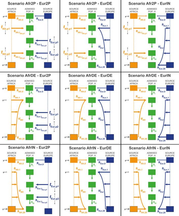
Nine competing scenarios for reconstructing the admixture history of African American ASW or Barbadian ACB populations descending from West European and West sub‐Saharan African source populations during the Transatlantic Slave Trade. “EUR” represents the Western European and “AFR” represents the West Sub‐Saharan African source populations for the admixed population H. See Table 1 and Section 2 for descriptions of the parameters of the scenarios

TABLE 1.

Parameter prior distributions for simulation with methis and Approximate Bayesian Computation historical inference

Parameter names	Parameter description	Prior distribution	Condition	Scenarios
s Afr,0 s Eur,0 = 1 − s Afr,0	Afr. source introgression rate at founding of H	Uniform [0,1]	—	All Scenarios
t Afr,p1 t Afr,p2	Times of the Afr. source introgression pulses p1 and p2	Uniform [0,20]	t Afr,p1 ≠ t Afr,p2	Afr2P Scenarios
s Afr, t Afr,p1 s Afr, t Afr,p2	Afr. source introgression rates of pulses Afr,p1 and Afr,p2	Uniform [0,1]	For all g, h g = 1 − s Afr,g ‐ s Eur,g in [0,1]	Afr2P Scenarios
t Eur,p1 t Eur,p2	Times of the Eur. source introgression pulses p1 and p2	Uniform [0,20]	t Eur,p1 ≠ t Eur,p2	Eur2P Scenarios
s Eur, t Eur,p1 s Eur, t Eur,p2	Eur. source introgression rates of pulses Eur,p1 and Eur,p2	Uniform [0,1]	For all g, h g = 1 − s Afr,g − s Eur,g in [0,1]	Eur2P Scenarios
s Afr,1	Afr. source introgression rate at the first generation after founding	Uniform [0,1]	For all g, h g =1 − s Afr,g − s Eur,g in [0,1]	AfrDE Scenarios
s Afr,20	Afr. source introgression rate in the present	Uniform [0, s Afr,1/3]	For all g, h g =1 − s Afr,g − s Eur,g in [0,1]	AfrDE Scenarios
u Afr	Steepness of the decrease in Afr. source introgression rates	Uniform [0,0.5]	—	AfrDE Scenarios
s Eur,1	Eur. source introgression rate at the first generation after founding	Uniform [0,1]	For all g, h g =1 − s Afr,g − s Eur,g in [0,1]	EurDE Scenarios
s Eur,20	Eur. source introgression rate in the present	Uniform [0, s Eur,1/3]	For all g, h g =1 − s Afr,g − s Eur,g in [0,1]	EurDE Scenarios
u Eur	Steepness of the decrease in Eur. source introgression rates	Uniform [0,0.5]	—	EurDE Scenarios
s Afr,1	Afr. source introgression rate at the first generation after founding	Uniform [0, s Afr,20/3]	For all g, h g =1 − s Afr,g − s Eur,g in [0,1]	AfrIN Scenarios
s Afr,20	Afr. source introgression rate in the present	Uniform [0,1]	For all g, h g =1 − s Afr,g − s Eur,g in [0,1]	AfrIN Scenarios
u Afr	Steepness of the increase in Afr. source introgression rates	Uniform [0,0.5]	—	AfrIN Scenarios
s Eur,1	Eur. source introgression rate at the first generation after founding	Uniform [0, s Eur,20/3]	For all g, h g =1 − s Afr,g − s Eur,g in [0,1]	EurIN Scenarios
s Eur,20	Eur. source introgression rate in the present	Uniform [0,1]	For all g, h g =1 − s Afr,g − s Eur,g in [0,1]	EurIN Scenarios
u Eur	Steepness of the increase in Eur. source introgression rates	Uniform [0,0.5]	—	EurIN Scenarios

Parameter list corresponds to the nine competing historical admixture scenarios described in Figure 1 and Section 2.

2.1. Nine competing complex admixture scenarios

2.1.1. Founding of the admixed population H

For all scenarios (Figure 1, Table 1), we chose a fixed time for the founding (generation 0, forward‐in‐time) of the target admixed population H occurring 21 generations before present, with admixture proportions s _Afr,0 and s _Eur,0 from either source population S respectively, African and European in our case, with s _Afr,0 + s _Eur,0 = 1, and s _Afr,0 in [0,1]. This duration corresponds roughly to the first arrival of European permanent settlers in the Americas in the late 15th century, considering 20 or 25 years per generation and the sampled generation born in the 1980s. Note that simulations with a parameter s _Afr,0 close to 0, or alternatively 1, corresponded to the founding of the population H from one source population only, therefore delaying the first “real” genetic admixture event to the next admixture event. Following founding, we considered three alternative scenarios for the admixture contribution of each source population S separately.

2.1.2. Admixture‐pulse(s) scenarios

For a given source population S, African or European, scenarios S‐2P considered two possible pulses of admixture into population H occurring respectively at time t _S,p1 and t _S,p2 distributed in [1,20] with t _S,p1 ≠ t _S,p2, with associated admixture proportion s _S,tS,p1 and s _S,tS,p2 in [0,1] satisfying, at all times t,$\sum _{S\in (Afr,Eur)}{s}_{S,t}\le 1$ (Figure 1, Table 1). Note that for one of either s _S,t values close to 0, the two‐pulses scenarios were equivalent to single‐pulse scenarios after the founding of H. Furthermore, for both s _S,t values close to 0, scenarios S‐2P were nested with scenarios where only the founding admixture pulse 21 generations ago was the source of genetic admixture. Alternatively, s _S,t parameter values close to 1 considered a virtual complete replacement of population H by population S at that time, thus obliterating all previous admixture events.

2.1.3. Recurring decreasing admixture scenarios

For a given source population S, scenarios S‐DE considered a recurring monotonically decreasing admixture from population S at each generation between generation 1 (after founding at generation 0) and generation 20 (sampled population) (Figure 1, Table 1). In these scenario, s _S,g, with g in [1,20], were the discrete numerical solutions of a rectangular hyperbola function over the 20 generations of the admixture process until present, as described in Note S2. In brief, this function is determined by the parameter u _S, the “steepness” of the curvature of the decrease, in [0,1/2], s _S,1, the admixture proportion from population S at generation 1 (after founding), in [0,1], and s _S,20, the last admixture proportion in the present, in [0,s _S,1/3]. Note that we chose the boundaries for s _S,20 in order to reduce the parameter space and nestedness among competing scenarios, by explicitly forcing scenarios S‐DE into substantially decreasing admixture processes. Furthermore, note that parameter u _S values close to 0 created pulse‐like scenarios of intensity s _S,1 occurring immediately after founding, followed by constant recurring admixture of intensity s _S,20 at each generation until present. Alternatively, parameter u _S values close to 1/2 created scenarios with linearly decreasing admixtures between s _S,1 and s _S,20 from population S at each generation after founding.

2.1.4. Recurring increasing admixture scenarios

For a given source population S, scenarios S‐IN mirrored the S‐DE scenarios by considering instead a recurring monotonically increasing admixture from population S (Figure 1, Table 1). Here, s _S,g, with g in [1,20], were the discrete numerical solutions of the same function as in the S‐DE decreasing scenarios (see above), flipped over time between generation 1 and 20. In these scenarios, s _S,20 was defined in [0,1] and s _S,1 in [0,s _S,20/3], and u, in [0,1/2], parametrized the “steepness” of the curvature of the increase. Note that S‐IN scenarios were nested with pulse‐like scenarios over the parameter space of u values, analogously to the nestedness of S‐DE and pulse‐like scenarios described above.

2.1.5. Combining admixture scenarios from either source populations

We combined these three scenarios to obtain nine alternative scenarios for the admixture history of population H (Figure 1, Table 1), with the only condition that, at each generation g in [1,20], parameters satisfied s _Afr,g + s _Eur,g + h _g = 1, with h _g, in [0,1] being the remaining contribution of the admixed population H to itself at generation g.

Four scenarios (Afr2P‐EurDE, Afr2P‐EurIN, AfrDE‐Eur2P, and AfrIN‐Eur2P) considered a mixture of pulse‐like and recurring admixture from each source. Three scenarios (Afr2P‐Eur2P, AfrDE‐EurDE, and AfrIN‐EurIN), considered symmetrical classes of admixture scenarios from either source. Two scenarios (AfrIN‐EurDE and AfrDE‐EurIN) considered mirroring recurring admixture processes. Importantly, this scenario design considered nested historical scenarios in specific parts of the parameter space.

2.2. Forward‐in‐time simulations with methis

Simulation of independent genetic markers under highly complex admixture histories is often not trivial under the coalescent and using classical existing software. Indeed, the coalescent generally assumes a different pedigree for each independent locus instead of a single pedigree having, in reality, produced all observed gene genealogies (see Wakeley et al., 2012). In this context, and because pedigrees are rarely known a priori, we developed methis, a C open‐source software package available at https://github.com/romain‐laurent/MetHis. methis simulates independent SNPs or microsatellite markers in an admixed population H under any version of the two source‐populations general model from Verdu and Rosenberg (2011), and calculates summary statistics of interest to the study of complex admixture processes (Note S1).

2.2.1. Simulating the admixed population, effective population size, and sampling individuals

At each generation, methis performs simple Wright‐Fisher (Fisher, 1922; Wright, 1931) forward‐in‐time simulations, individual‐centered, in a panmictic population of diploid effective size N _g. For a given individual in the population H at the following generation (g + 1), methis independently draws each parent from the source populations with probability s _S,g (Figure 1, Table 1), or from population H with probability $h_g=1‐\sum _{S\in (Afr,Eur)}{s}_{S,g}$, randomly builds a haploid gamete of independent markers for each parent, and pairs the two constructed gametes to create the new individual.

Here, we decided to neglect mutation over the 21 generations of admixture considered. This was reasonable when studying relatively recent admixture histories and considering independent genotyped SNP markers. For users interested in microsatellite variation and longer admixture histories, methis readily implements a standard general stepwise mutation model allowing for insertion or deletion (Estoup et al., 2002), with parameters set by the user (Note S1).

To focus on the admixture process itself without excessively inflating the parameter space, we considered, for each of the nine competing scenarios, the admixed population H with constant effective population size N _g = 1000 diploid individuals. Nevertheless, note that methis readily allows the user to parametrize, instead, stepwise or continuous changes in effective population size over time (Note S1).

After each simulation, we randomly drew individual samples matching sample‐sizes in our observed data set (see Section 2.4.3). We sampled individuals until our sample set contained no individuals related at the first degree cousin within each population and between population H and either source population, based on explicit parental flagging during the last two generations of the simulations. Note that this is done to best mimic, a priori, the observed case‐study data sets, but excluding related individuals is an option set by the user in methis (Note S1).

2.2.2. Simulating source populations

methis, in its current form, does not allow simulating the source populations for the admixture process modeled in Verdu and Rosenberg (2011). Simulating source populations can be done separately using existing genetic data simulation software such as fastsimcoal2 sequential coalescent (Excoffier et al., 2013; Excoffier & Foll, 2011).

Another possibility to simulate source populations emerges if genetic data is already available for the known source populations, as it is the case in our case studies of enslaved‐African descendants in the Americas (see Section 2.4.3). We considered here that the African and European source populations were very large populations at the drift‐mutation equilibrium, accurately represented by the Yoruban YRI and British GBR data sets here investigated (see Section 2.4.3). Therefore, we first built two separate data sets each comprising 20,000 haploid genomes of 100,000 independent SNPs, each SNP being randomly drawn in the site frequency spectrum (SFS) observed for the YRI and GBR data sets respectively. These two data sets were used as fixed gamete reservoirs for the African and European sources separately, at each generation of the forward‐in‐time admixture process. From these reservoirs, we built an effective individual gene pool of diploid size N _g, by randomly pairing gametes avoiding selfing. These virtual source populations provided the parental pool for simulating individuals in the admixed population H with methis, at each generation. Thus, while our gamete reservoirs were fixed, the parental genetic pools were randomly built anew at each generation. Again, note that this is not necessary to the implementation of methis for investigating complex admixture histories; source populations can be simulated separately by the user at will.

2.3. Summary statistics

methis is designed to work in an ABC inference framework and, thus, can calculate numerous summary statistics. A complete list of summary statistics can be found in Note S1. Below are the summary statistics considered in our case studies, in particular introducing the distribution of admixture fractions in population H, as summary statistics for ABC inference.

2.3.1. The distribution of admixture fractions as a set of summary statistics

Most methods developed to estimate individual admixture fractions from genetic data (e.g., Alexander et al., 2009), are computationally intensive, and are thus difficult to iterate over large sets of simulated genetic data. This explains why they have not been routinely used in ABC in the past, despite being theoretically highly informative for admixture inference (Gravel, 2012; Verdu & Rosenberg, 2011).

Here, we propose, and implement in methis, an efficient way to use estimated individual admixture fractions as summary statistics for ABC inference, based on allele sharing dissimilarity (ASD) (Bowcock et al., 1994) and multidimensional scaling (MDS). For each simulated data set, we first calculated a pairwise interindividual ASD matrix using our implementation of the asd software (https://github.com/szpiech/asd), using all pairs of sampled individuals and all markers. Then we projected in two dimensions this pairwise ASD matrix with classical unsupervised metric MDS using the “cmdscale” function in R. We expected individuals in population H to be dispersed along an axis joining the centroids of the proxy source populations on the two‐dimensional MDS plot. We projected population H’s individuals orthogonally onto this axis, and calculated each individual's relative distance to each centroid. We considered this measure as an estimate of individual average admixture level from either source. Note that by doing so, some individuals might show “admixture fractions” higher than one, or lower than zero, as they might be projected on the other side of a source‐population's centroid when being genetically close to 100% from this source population. Under an ABC framework, this was not a difficulty since this may happen also with the real data a priori, and the goal of ABC is to use summary statistics that mimic the observed ones.

This individual admixture estimation method has been shown to be highly concordant with cluster membership fractions as estimated with STRUCTURE (Falush et al., 2003) or ADMIXTURE (Alexander et al., 2009) in real data analyses (e.g., Verdu et al., 2017). We confirmed these previous findings since we obtained a Spearman's rank correlation (calculated using the cor.test function in R), of ρ = 0.950 (p‐value <2.10⁻¹⁶) and ρ = 0.977 (p‐value <2.10⁻¹⁶) between admixture estimates based on ASD‐MDS and on ADMIXTURE, for the two case‐study data sets here explored (Figure S2).

We used the mean, mode, variance, skewness, kurtosis, minimum, maximum, and all 10%‐quantiles of the admixture distribution in population H, as 16 separate summary statistics for ABC inference.

2.3.2. Within population summary statistics

We calculated marker by marker heterozygosities (Nei, 1978), and we considered the mean and variance of this quantity across markers in the admixed population as two separate summary statistics for ABC inference. In addition, we considered the mean and variance of ASD values across pairs of individuals within population H.

2.3.3. Between populations summary statistics

We calculated multilocus pairwise F _ST (Weir & Cockerham, 1984) between population H and each source population respectively. Furthermore, we calculated the mean ASD between individuals in population H and individuals in each source population, separately. Finally, we calculated the f₃ statistics (Patterson et al., 2012).

2.4. Approximate Bayesian Computation

methis provides, as outputs, vectors of scenario parameters and corresponding vectors of summary statistics in reference tables ready to be used with the machine‐learning ABC R packages abc (Csilléry et al., 2012), and abcrf (Pudlo et al., 2016; Raynal et al., 2019).

2.4.1. Simulating by randomly drawing parameter values from prior distributions

We performed methis simulations under each of the nine competing scenarios (Figure 1), drawing the corresponding scenario‐parameters in prior distributions detailed in Table 1 and automatically generated by methis parameter‐generator tools (Note S1).

2.4.2. Complex admixture scenario‐choice with Random‐Forest ABC

For ABC scenario‐choice, we performed 10,000 independent methis simulations for each of the nine competing scenarios. To mimic our case study data sets (see Section 2.4.3), we simulated 100,000 SNPs and sampled 50 individuals in population H, and 90 and 89 individuals respectively in the African and European source populations. Using 27 cores and the above design, we performed the 90,000 simulations with methis in four days, with 2/3 of that time for summary statistics calculation only (Note S1).

We used Random‐Forest ABC for scenario‐choice implemented in the “abcrf” function of the abcrf package to obtain the cross‐validation table and associated prior error rate using an out‐of‐bag approach. We considered a uniform prior probability for the nine competing models. We considered 1,000 decision trees in the forest after visually checking that error‐rates converged appropriately, using the “err.abcrf function”. RF‐ABC cross‐validation procedures using groups of scenarios were conducted using the group definition option in the “abcrf” function (Estoup et al., 2018). Finally, the relative importance of each summary statistic to the scenario‐choice cross‐validation was computed using the “abcrf” function.

We explored scenario‐choice erroneous assignation due to scenario nestedness in the parameter space, by considering 1000 randomly chosen simulations per scenario as pseudo‐observed data. We trained the RF algorithm based on the 9000 remaining simulations per scenario using the “abcrf” function as described above, which provided highly similar results as when considering 10,000 simulations per scenario (results not shown). We then used the “predict.abcrf” function to perform scenario‐choice independently for each of the 1,000 simulated pseudo‐observed data with known parameter vectors.

To empirically evaluate the power of the RF‐ABC scenario‐choice to distinguish complex admixture processes, we conducted similar cross‐validations procedures based on additional 10,000 simulations per scenario for 50,000 and, separately, 10,000 SNPs, instead of 100,000 SNPs (180,000 additional simulations in total).

Furthermore, using 100,000 SNPs, we produced 90,000 additional simulations and performed cross‐validations, considering a five‐times smaller sample set, with 10 sampled individuals in population H (instead of 50 as previously) and 18 individuals in each source population (instead of 90 and 89).

2.4.3. Case‐study population genetics data sets

We investigated, as two separate study‐cases, the admixture histories of the African American (ASW) and Barbadian (ACB) population samples from the 1000 Genomes Project Phase 3 (1000 Genomes Project Consortium, 2015). Previous studies identified, within the same database, the West European Great‐Britain (GBR) and the West African Yoruba (YRI) populations as reasonable proxies for the sources of both ACB and ASW, consistent with the macro‐history of the Transatlantic Slave‐Trade (Baharian et al., 2016; Martin et al., 2017; Verdu et al., 2017).

Individuals in the 1000 Genomes Project were a priori sampled to be family unrelated. To avoid confounding factors due to cryptic relatedness in this sample set compared to methis simulations, we excluded individuals more closely related than first‐degree cousins in the four populations separately using RELPAIR (Epstein, Duren, & Boehnke, 2000), as previously done (Verdu et al., 2017). We also excluded the three ASW individuals showing traces of Native American or East‐Asian admixture, as reported in previous studies (Martin et al., 2017). Among the remaining individuals we randomly drew 50 individuals in the target admixed ACB and ASW, respectively, and included the remaining 90 YRI individuals and 89 GBR individuals.

We extracted biallelic polymorphic sites (SNPs as defined by the 1000 Genomes Project Phase 3) from the merged ACB+ASW+GBR+YRI data set, excluding singletons. Since methis could only simulate independent markers, we LD‐pruned the ACB and ASW SNP‐sets using the PLINK (Purcell et al., 2007) “‐‐indep‐pairwise” option with a sliding window of 100 SNPs, moving in increments of 10 SNPs, with an r² threshold of 0.1. Finally, we randomly drew 100,000 SNPs from the remaining SNP‐set.

2.4.4. Prior‐checking of simulations’ fit to the case‐study data sets

We plotted prior distributions of each summary statistic and visually verified that the observed summary statistics for the ACB and ASW respectively fell within the simulated distributions. Then, we explored the first four axes of a principal component analysis (PCA) computed with the “princomp” function in R, using the 24 summary statistics and all 90,000 simulations, and visually checked that observed summary statistics were within the cloud of simulated statistics. Finally, we performed a goodness‐of‐fit approach using the “gfit” function from the abc package in R, with 1,000 replicates and tolerance level 0.01.

2.4.5. RF‐ABC scenario‐choice for the admixture history of ACB and ASW populations

For the ACB and ASW observed data separately, we performed scenario‐choice prediction and estimation of posterior probabilities of the winning scenario using the “predict.abcrf” function in the abcrf package, using the complete simulated reference table for training the Random‐Forest algorithm (100,000 SNPs, 50 individuals in population H, 90 and 89 individuals in the African and European sources, respectively).

2.4.6. Posterior parameter estimation with Neural‐Network ABC

It is difficult to estimate jointly the posterior distribution of all model parameters with RF‐ABC (Raynal et al., 2019). Furthermore, although RF‐ABC performs satisfactorily well with an overall limited number of simulations under each model (Pudlo et al., 2016), posterior parameter estimation with other ABC approaches, such as simple rejection (Pritchard et al., 1999), regression (Beaumont et al., 2002; Blum & François, 2010) or Neural‐Network (NN) (Csilléry et al., 2012), require substantially more simulations a priori. Therefore, we performed, for posterior parameter estimations, 90,000 additional simulations, for a total of 100,000 simulations under the best scenarios identified with RF‐ABC for the ACB and ASW separately. For comparison purposes, we also performed an additional 90,000 simulations (for a total of 100,000 simulations) under the loosing scenario Afr2P‐Eur2P (see Results), and conducted anew the below parameter estimation and error evaluation procedures for this scenario.

2.4.7. Neural‐Network tolerance level and number of neurons in the hidden layer

We determined empirically the NN tolerance level (i.e., the number of simulations to be included in the NN training), and number of neurons in the hidden layer. Indeed, the NN needs a substantial amount of simulations for training, and there is also a risk of overfitting posterior parameter estimations when considering too large a number of neurons in the hidden layer. However, there are no absolute rules for choosing both numbers (Csilléry et al., 2012; Jay et al., 2019).

Therefore, we tested four different tolerance levels to train the NN for parameter estimation (0.01, 0.05, 0.1, and 0.2), and a number of neurons that ranged between four and seven (the number of free parameters in the winning scenarios, see Results). For each pair of tolerance level and number of neurons, we conducted cross‐validation with 1000 randomly chosen simulated data sets that we used, in turn, as pseudo‐observed data with the “cv4abc” function in the package abc. We compared the median point‐estimate of each posterior parameter $({\widehat{\theta }}_i)$ to the true parameter value used for simulation $({\theta }_i)$. The cross‐validation parameter prediction error was then calculated across the 1000 separate posterior estimations for pseudo‐observed data sets for each pair of tolerance level and number of neurons, and for each parameter ${\theta }_i$, as $\sum _1^{1000}{({\widehat{\theta }}_i‐{\theta }_i)}^2/(1000\times Variance({\theta }_i))$, using the “summary.cv4abc” function in the package abc (Csilléry et al., 2012). Results showed that, a priori, all numbers of neurons considered perform very similarly for a given tolerance level. Furthermore, results showed that considering the 1% closest simulations to the pseudo‐observed ones reduced the average error for each number of neurons tested. Thus, we decided to opt for four neurons in the hidden layer and a 1% tolerance level for training the NN in all subsequent parameter inference, in order to avoid overfitting.

2.4.8. Estimation of scenario‐parameters’ posterior distributions

We jointly estimated the posterior distributions of scenario parameters for the ACB and ASW admixed populations separately, using NN‐ABC “neuralnet” method option in the function “abc”, with logit‐transformed (“logit” transformation option) summary statistics using a 1% tolerance level and four neurons in the hidden layer.

2.4.9. Posterior parameter estimation error

We evaluated the posterior error of the NN‐ABC approach in the vicinity of our observed data rather than randomly on the entire parameter space. To do so, we first identified the 1000 simulations closest to the real data by setting a tolerance level of 1% with the "abc" function, for the ACB and ASW respectively. Then, we performed 1000 separate NN‐ABC parameter estimations, each parameterized as described above, using in turn the remaining 99,999 simulations as reference tables, and recorded the median point estimate for each parameter. We then compared each parameter estimate with the true parameter used for each one of the 1000 pseudo‐observed target data and provided three types of error measurements. The mean‐squared error scaled by the variance of the true parameter $\sum _1^{1000}{({\widehat{\theta }}_i‐{\theta }_i)}^2/(1000\times Variance({\theta }_i))$, as previously (Csilléry et al., 2012); the mean‐squared error $\sum _1^{1000}{({\widehat{\theta }}_i‐{\theta }_i)}^2/1000$, which allowed to compare errors for a given scenario and parameter between the ACB and ASW analyses; and the mean absolute error $\sum _1^{1000}|{\widehat{\theta }}_i‐{\theta }_i|/1000$, which provided a more intuitive parameter estimation error. For comparison, we conducted the above analysis using instead parameters estimated under the losing scenario Afr2P‐Eur2P.

2.4.10. 95% credibility interval accuracy

We evaluated a posteriori, if, in the vicinity of the two observed data sets respectively, the lengths of the estimated 95% confidence intervals (CI) for each parameter were accurately estimated or not (e.g., Jay et al., 2019). To do so, we calculated how many times the true parameter $({\theta }_i)$ was found inside the estimated 95% CI (2.5% quantile $(\widehat{{\theta }_i}))$; 97.5% quantile $(\widehat{{\theta }_i})$), among the 1000 out‐of‐bag NN‐ABC posterior parameter estimations. For each parameter, if fewer than 95% of the true parameter values were found inside the 95% CI estimated for the observed data, we considered the length of this credibility interval as underestimated which was indicative of a nonconservative behaviour of the parameter estimation. Alternatively, if more than 95% of the true parameter values were found inside the estimated 95% CI, we considered its length as overestimated, indicative of an excessively conservative behaviour of parameter estimation. For comparison, we conducted the above analysis using instead parameters estimated under the losing scenario Afr2P‐Eur2P.

2.4.11. Comparing the accuracy of posterior parameter estimations using NN, RF, or rejection ABC

We compared four ABC posterior parameter estimation methods: NN‐ABC estimation of the parameters taken jointly as a vector (as described in the above procedures), NN‐ABC estimation of the parameters taken in turn separately, RF‐ABC estimation of the parameters which also considers parameters in turn and separately (Raynal et al., 2019), and simple Rejection‐ABC estimation for each parameter separately (Pritchard et al., 1999). For each method, we used in turn the 1000 simulations closest to the real data as pseudo‐observed data and the 99,999 remaining simulations as reference tables. We considered the same parameters for the NN, and we used 500 decision trees for the RF to limit the computational cost at little accuracy cost a priori. We computed the three types of errors and the accuracies of the 95% CI for each ABC method as described above.

3. RESULTS

3.1. Complex admixture scenarios cross‐validation with RF‐ABC

We trained the RF‐ABC scenario‐choice algorithm using 1000 trees, which guaranteed the convergence of the scenario‐choice prior error rates (Figure S3). Based on this training, the complete out‐of‐bag cross‐validation matrix showed that the nine competing scenarios of complex historical admixture (Figure 1, Table 1) could be relatively reasonably distinguished despite the high level of nestedness of the scenarios here considered (Figure 2). Indeed, we calculated an out‐of‐bag prior error rate of 32.41%, considering each of the 90,000 simulations, in turn, as out‐of‐bag pseudo‐observed target data sets, compared to a prior probability of 88.89% to erroneously select a scenario. Furthermore, we found that cross‐validation probabilities of identifying the correct scenario ranged from 55.17% (prior probability = 11.11% for each competing scenario), for the two‐pulses scenarios from both the African and European sources (Afr2P‐Eur2P), to 77.71% for the scenarios considering monotonically decreasing recurring admixture from both sources (AfrDE‐EurDE).

FIGURE 2.

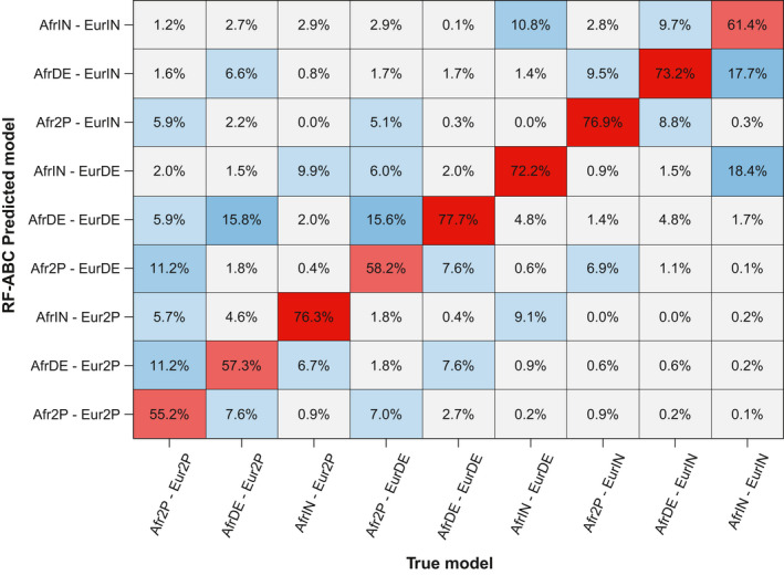
Random‐Forest Approximate Bayesian Computation scenario‐choice cross‐validation. Heat map of the out‐of‐bag cross‐validation results considering each of the 10,000 simulations per each of the nine competing scenarios (Figure 1, Table 1) in turn as pseudo‐observed target for RF‐ABC model‐choice. Prior probability of correctly choosing a given scenario was 11%. Out‐of‐bag prior error rate was 32.41%. RF‐ABC scenario‐choice performed using 1000 decision trees and 24 summary statistics (see Section 2)

The probability, for a given admixture scenario, of choosing any one alternative (wrong) scenario was on average 4.05% across the eight alternative scenarios, ranging from 2.79% for the AfrDE‐EurDE scenario, to 5.60% for the Afr2P‐Eur2P scenario (Figure 2). However, cross‐validation assignment errors, for a given true scenario, were not uniformly distributed across the eight alternative scenarios. Instead, Figure 2 shows that assignment errors were relatively less frequent for classes of scenarios a priori more differentiated from the true scenario. For instance, the Afr2P‐Eur2P true scenarios were less often confused (10.7%) with scenarios encompassing recurring admixture from both source populations (AfrDE‐EurDE, AfrIn‐EurDE, AfrDE‐EurIN, AfrIN‐EurIN), than with scenarios containing pulses of admixture from one source population (34.0%; AfrDE‐Eur2P, Afr2P‐EurDE, AfrIN‐Eur2P, Afr2P‐EurIN). Furthermore, note that AfrDE‐EurDE scenarios were rarely confused (3.8%) with recurring scenarios containing at least one admixture increase (AfrIN‐EurDE, AfrDE‐EurIN, AfrIN‐EurIN). Across the nine nested competing scenarios of highly complex admixture processes, these results showed a strong discriminatory power of RF‐ABC scenario‐choice a priori.

In cross‐validation analyses of groups of scenarios (Estoup et al., 2018), monotonically recurring admixture scenarios (AfrDE‐EurDE, AfrDE‐EurIN, AfrIN‐EurDE, AfrIN‐EurIN) could be well distinguished from scenarios considering two possible pulses after the founding event (Afr2P‐Eur2P, Afr2P‐EurDE, Afr2P‐EurIN, AfrDE‐Eur2P, AfrIN‐Eur2P). Indeed, we found an out‐of‐bag prior error rate of 13.85%, and cross‐validation probabilities of identifying the correct group of scenarios of 86.08% and 86.23% for the two groups, respectively.

Detailed investigation of cross‐validation results showed that inaccuracies of RF‐ABC scenario‐choices occurred mainly in spaces of values of parameters where scenarios were highly nested and, in fact, close biologically (Figure 2). As expected, scenario‐choice increasingly mistook the AfrDE‐EurDE scenarios for scenarios containing two admixture pulses (Afr2P‐Eur2P, Afr2P‐EurIN, AfrIN‐Eur2P), as values of u _Afr and u _Eur were closer to 0, regardless of the values of introgression rates (Figure S4a). Intuitively for the S‐DE scenarios, values of the parameter u close to 0 corresponded to steeper decreases of recurring admixture over time, which increased scenario‐choice confusion with pulse‐like scenarios. Simulation with u‐values closer to 0.5 corresponded to linearly decreasing admixture over time and could hardly be confounded with pulse‐like scenarios. Furthermore, the scenario‐choice increasingly confused, as expected regardless of introgression values, Afr2P‐Eur2P scenarios with recurring increasing admixture scenarios (AfrIN‐EurIN, AfrDE‐EurIN, AfrIN‐EurDE), as the time of the second admixture pulse from Europe or Africa became more recent (Figure S4b).

Most importantly, RF‐ABC scenario‐choice power to discriminate among complex admixture processes a priori was not strongly affected by the numbers of markers considered. Indeed, we found an out‐of‐bag prior error of 33.53% and 37.93% (instead of 32.41%), considering respectively 50,000 and 10,000 SNPs, instead of 100,000, together with a very similar distribution of correct and mistaken cross‐validation assignments among scenarios (Figures S5a,b). Finally, dividing by five the sample sizes in population H and each source population increased, as expected, the cross‐validation error rate (48.39%). Nevertheless, all scenarios continued to be correctly identified three to six times more often than expected a priori, and the distribution of erroneous predictions remained similar to previously (Figure S5c).

Altogether, these results showed that RF‐ABC scenario‐choice can be successfully used to distinguish highly complex admixture models even when substantially less genetic and sample data are considered. Finally, the estimated relative importance of each summary statistic for RF‐ABC scenario‐choice showed that the minimum, maximum, 10%‐quantile, 90%‐quantile, variance, and skewness of the distribution of admixture fractions among individuals in the admixed population were, among the 24 summary statistics used, the most informative statistics for our scenario‐choice cross validation results (Figure S6).

3.2. Simulating data similar to the observed data with methis

Using methis, we produced 90,000 vectors of 24 summary statistics each, overall highly consistent with the observed ones for the ACB and the ASW populations. First, each observed statistic was visually reasonably well simulated under the nine competing scenarios here considered (Figure S7). Second, the observed data each fell into the simulated sets of 24 summary statistics projected in the first four PCA dimensions (Figure S8). Finally, the observed vectors of summary statistics were not significantly different (p‐value = 0.468 and 0.710, for the ACB and ASW respectively) from the simulated ones using a goodness‐of‐fit approach (Figure S9). Therefore, we successfully simulated data sets producing sets of summary statistics reasonably close to the observed ones, despite considering constant effective population sizes, using fixed virtual source population genetic pool‐sets, and neglecting mutation during the admixture process.

3.3. Random‐Forest ABC scenario‐choice for the history of ACB and ASW populations

We performed RF‐ABC scenario‐choice separately for the admixture history of the ACB and the ASW populations, to evaluate whether our methis‐ABC method could identify subtle differences in the history of both populations having experienced the TAST under the British colonial empire (Baharian et al. 2016; Martin et al. 2017). For the ACB, Figure 3 shows that the majority of votes (53.1%) went to an admixture scenario AfrDE‐EurDE with a posterior probability of the winning scenario of 60.3%. This posterior probability was above the mean posterior probability obtained when the wrong scenario was chosen for the 1000 AfrDE‐EurDE simulations closest to the observed one (56.8%, SD = 11.6%, for 37 simulations wrongly assigned in total). The second most chosen scenario was the AfrDE‐Eur2P scenario. However, this scenario was voted for 3.5 times less often than the winning scenario AfrDE‐EurDE, gathering 15.1% of the 1000 votes, only slightly above the 11.11% prior probability for the nine competing scenarios (Figure 3; Table S1).

FIGURE 3.

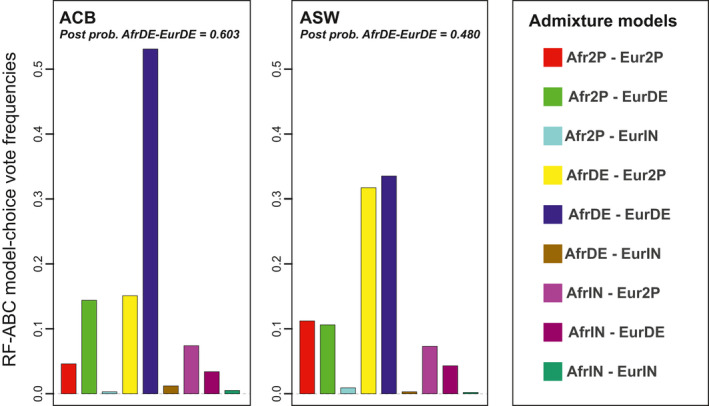
Random‐Forest Approximate Bayesian Computation scenario‐choice predictions for the ACB (left panel) and ASW (right panel) populations. Nine competing scenarios were compared, each with 10,000 simulations (Figure 1, Table 1), and 1,000 decision trees were considered in the scenario‐choice prediction, respectively for each population

RF‐ABC scenario‐choice results were less decisive for the ASW (Figure 3). The AfrDE‐EurDE scenario also gathered the majority of votes, albeit with lower posterior probability than for the ACB (33.5% of 1000 votes, with posterior probability = 48.0%). This posterior probability was slightly below the average posterior probability obtained when the wrong scenario was chosen for the 1000 AfrDE‐EurDE simulations closest to the ASW observed data (50.7%, SD = 7.9%, for 192 simulations wrongly assigned). The second most chosen scenario, AfrDE‐Eur2P, was only slightly less chosen with 31.7% of the votes (Figure 3, Table S1). Altogether these results denoted an ambiguity of the RF‐ABC scenario‐choice in the part of the space of summary statistics occupied by the ASW.

Considering only these two best scenarios to train the RF and reconducting ABC scenario‐choice improved the scenario discrimination in favor of the AfrDE‐EurDE scenario. While we found, again, only a slight majority of votes (51.8%) in favour of the AfrDE‐EurDE scenario, the posterior probability for this scenario was substantially increased to 57.9%, thus above the average posterior probability threshold calculated previously (50.7%). This indicated that the AfrDE‐EurDE scenario best explained the ASW observed genetic patterns, despite overall limited discriminatory power of our approach in the ambiguous part of the space of summary statistics occupied by this population.

3.4. Neural‐Network ABC parameter inference accuracy

For the ACB under the AfrDE‐EurDE scenario (Figure 4a, Table 2), we conducted a NN‐ABC posterior parameter inference considering four neurons and a tolerance level of 1% (Table S2). We found that the two recent admixture intensities from Africa and Europe (s _Afr,20 and s _Eur,20, respectively), and the steepness of the European recurring introgression decrease (u _Eur), had sharp posterior densities clearly distinct from their respective priors. Note that the cross‐validation error on these parameters in the vicinity of our real data were low (average absolute error 0.02744, 0.0044, and 0.1084, respectively for s _Afr,20, s _Eur,20, and u _Eur) (Table 3), and lengths of 95% CI reasonably accurate (96.4%, 94.4%, 94.1% of 1000 cross‐validation true parameter values fell into estimated 95% CI, Table S3).

FIGURE 4.

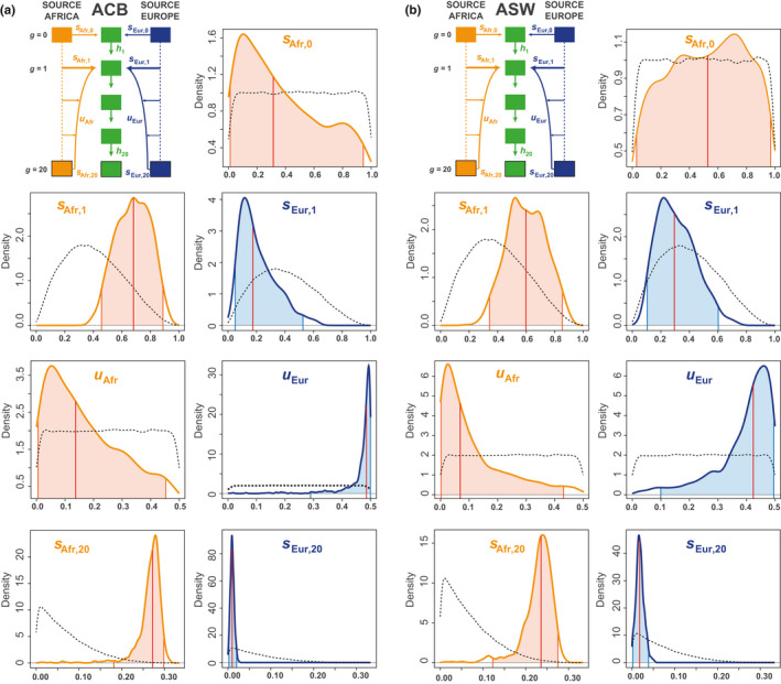
Neural‐Network Approximate Bayesian Computation posterior parameters estimated densities under the winning scenario AfrDE‐EurDE, for (a) the ACB and (b) the ASW populations. Median posterior point estimates are indicated by the red vertical line, 95% credibility intervals are indicated by the colored area under the posterior density‐curve (Table 2). All posterior parameter estimations were conducted using 100,000 simulations under scenario AfrDE‐EurDE, a 1% tolerance rate (1000 simulations), 24 summary statistics, logit transformation of all parameters, and four neurons in the hidden layer (see Section 2). For all parameters separately, densities were plotted with 1000 points, a Gaussian kernel, and were constrained to the prior limits. Posterior parameter densities are indicated by a solid line; prior parameter densities are indicated by black dotted lines

TABLE 2.

Neural‐Network Approximate Bayesian Computation posterior parameter weighted distributions under the winning scenario AfrDE‐EurDE, for the ACB and ASW populations

Admixed population	AfrDE‐EurDE parameters	Median	Mean	Mode	95% credibility interval
ACB	s Afr,0	0.3097	0.3747	0.1121	[0.0116; 0.9347]
	s Afr,1	0.6797	0.6769	0.6813	[0.4577; 0.8880]
	s Afr,20	0.2707	0.2655	0.2788	[0.1985; 0.2967]
	u Afr	0.1409	0.1684	0.0508	[0.0041; 0.4507]
	s Eur,1	0.1807	0.2160	0.1158	[0.0542; 0.5525]
	s Eur,20	0.0100	0.0102	0.0093	[0.0018; 0.0200]
	u Eur	0.4858	0.4627	0.4929	[0.1886; 0.4992]
ASW	s Afr,0	0.5258	0.5124	0.7015	[0.0262; 0.9758]
	s Afr,1	0.6006	0.6026	0.6081	[0.3506; 0.8581]
	s Afr,20	0.2352	0.2286	0.2385	[0.1222; 0.2714]
	u Afr	0.0662	0.1105	0.0253	[0.0025; 0.4393]
	s Eur,1	0.2917	0.3080	0.2203	[0.1048; 0.5951]
	s Eur,20	0.0180	0.0189	0.0157	[0.0022; 0.0389]
	u Eur	0.4250	0.3966	0.4567	[0.1077; 0.4950]

All posterior parameter estimations were conducted using 100,000 simulations under the AfrDE‐EurDE scenario (Figure 1, Table 1), a 1% tolerance rate (1,000 simulations), 24 summary statistics, logit transformation of all parameters, and four neurons in the hidden layer (see Section 2).

TABLE 3.

Neural‐Network Approximate Bayesian Computation posterior parameter errors under the winning scenario AfrDE‐EurDE, for the ACB and ASW populations

AfrDE‐EurDE parameters	ACB			ASW
	Av. absolute error	Mean‐square error	Mean‐square error/var.	Av. absolute error	Mean‐square error	Mean‐square error/var.
s Afr,0	0.2530	0.0857	1.0070	0.2444	0.0805	1.0081
s Afr,1	0.1206	0.0216	0.8533	0.1158	0.0197	0.9259
s Afr,20	0.02744	0.0012	0.4162	0.0219	0.0007	0.4773
u Afr	0.1166	0.0198	0.9974	0.1254	0.0216	0.9757
s Eur,1	0.0952	0.0164	1.0526	0.1001	0.0157	1.0152
s Eur,20	0.0044	0.0001	0.6452	0.0069	0.0001	0.6623
u Eur	0.1084	0.0174	0.9431	0.1021	0.0153	0.8036

For each target population separately, we conducted cross‐validation by considering in turn 1000 separate NN‐ABC parameter inferences each using in turn one of the 1000 closest simulations to the observed ACB (or ASW) data as the target pseudo‐observed simulation. All posterior parameter estimations were conducted using 100,000 simulations under the AfrDE‐EurDE scenario (Figure 1, Table 1), a 1% tolerance rate (1000 simulations), 24 summary statistics, logit transformation of all parameters, and four neurons in the hidden layer (see Section 2). Median was considered as the point posterior parameter estimation for all parameters. First column provides the average absolute error; second column shows the mean‐squared error; third column shows the mean‐squared error scaled by the parameter's observed variance (see Section 2 for error formulas)

Furthermore, the two ancient admixture intensities from Africa and Europe at generation 1 (s _Afr,1 and s _Eur,1, respectively), also had posterior densities apparently distinguished from their prior distributions, but both had much wider 95% CI (Figure 4a, Table 2). Consistently, we found a slightly increased posterior parameter error in this part of the parameter space for both parameters, with average absolute error equal to 0.121 and 0.095, respectively for s _Afr,1 and s _Eur,1 (Table 3). Nevertheless, note that 95.8% and 94.7% of 1000 cross‐validation true values for those two parameters fell into the estimated 95% CI (Table S3). This showed that information was somewhat lacking in our set of summary statistics for a more accurate point estimation of these parameters, albeit our method was reasonably conservative for these estimations.

Interestingly‐, we found that accurate posterior estimation of the steepness of the African recurring introgression decrease (u _Afr) was difficult. Indeed, the posterior density of this parameter showed a tendency towards small values only slightly departing from the prior, indicative of a limit of our method to estimate this parameter (Figure 4a, Table 2). Finally (Figure 4a, Table 2), we found that we had virtually no information to estimate the founding admixture proportions from Africa and Europe at generation 0, as our posterior estimates barely departed from the prior, and as associated mean absolute error was high (0.2530, Table 3). Nevertheless, our method seemed to be performing reasonably conservatively for these two latter parameters (95.6% and 95.3% of 1000 cross‐validation true parameter values fell into estimated 95% CI, Table S3).

For the ASW under the AfrDE‐EurDE scenario, our posterior parameter estimation results were overall less accurate compared to those obtained for the ACB population, as indicated by overall larger CI and cross‐validation errors (Figure 4b, Table 2, Table 3, Table S3). This was consistent with the more ambiguous RF‐ABC scenario‐choice results obtained for this population (Figure 3).

Note that, we conducted the above analyses under the losing scenario Afr2P‐Eur2P instead, for comparison. We found, as expected, that parameters and 95% CI were very poorly estimated for all parameters under this scenario (Tables S4 and S5). This indicated, consistently, that no information was available in the ACB or ASW data for accurate and conservative estimation of the parameters of the losing scenario Afr2P‐Eur2P using ABC.

3.5. Comparing NN, RF, and Rejection ABC posterior parameter estimation accuracy

The three types of posterior parameter estimation errors (scaled mean‐squared error, mean‐squared error, average absolute error) were systematically lower for the two NN methods (joint or independent posterior parameter estimations) than for the RF and Rejection independent posterior parameter estimations (Table 4). Altogether, these results showed that considering the NN estimation for parameters taken jointly as a vector was overall preferable, since it further allowed the joint interpretation of parameter values estimated a posteriori with little accuracy loss.

TABLE 4.

Approximate Bayesian Computation mean posterior parameter errors over all parameters under the winning Scenario AfrDE‐EurDE, for the ACB and ASW populations separately, using four different methods: NN estimation of the parameters taken jointly as a vector, NN estimation of the parameters taken separately, Random‐Forest (parameters taken separately), and Rejection (parameters taken separately)

Posterior parameter estimation ABC method	ACB			ASW
	Av. absolute error	Mean‐squared error	Mean‐squared error/var.	Av. absolute error	Mean‐squared error	Mean‐squared error/var.
NN joint	0.1037	0.0232	0.8450	0.1024	0.0219	0.8383
NN independent	0.1032	0.0236	0.8294	0.1025	0.0225	0.8344
RF independent	0.1042	0.0246	0.8534	0.1036	0.0233	0.8697
Rejection independent	0.1071	0.0238	0.9299	0.1050	0.0223	0.8951

For each target population separately and for each method, we conducted an out‐of‐bag cross validation by considering in turn 1000 separate parameter inferences each using one of the 1000 closest simulation to the observed ACB (or ASW) data as the target pseudo‐observed data set. All posterior parameter estimations were conducted using the remaining 99,999 simulations under the AfrDE‐EurDE scenario (Figure 1, Table 1), a 1% tolerance rate (i.e., 1000 simulations), 24 summary statistics, logit transformation of all parameters, four neurons in the hidden layer per Neural‐Network and 500 trees per Random‐Forest. Median was considered as the point posterior parameter estimation for all parameters. The first column provides the average absolute error; second column shows the mean‐squared error; third column shows the mean‐squared error scaled by the parameter's observed variance (see Section 2 for error formulas).

The lengths of 95% CI estimated with NN joint parameter estimation were, across all parameters, more accurate than those obtained with all other methods with, on average, 95.1% and 95.2% of true parameter values falling within the estimated 95% CI, for the ACB and ASW respectively (Table S3). Furthermore, the lengths of 95% CI estimated with NN and RF independent posterior parameter estimations were systematically underestimated, with less than 94% of the true parameter values falling into the estimated 95% CI. Finally, the lengths of 95% CI estimated with the Rejection method were also rather accurately estimated, although on average slightly overestimated compared to the NN joint estimation with, on average, 95.5% of the 1000 cross‐validation true parameter values within the estimated 95% CI for the ACB, and 95.8% for the ASW.

3.6. Admixture histories of the African American ASW and Barbadian ACB

Figure 5 visually synthesizes the estimated posterior parameters of the complex admixture scenarios reconstructed with the methis‐ABC framework, and associated 95% CI (Table 2).

FIGURE 5.

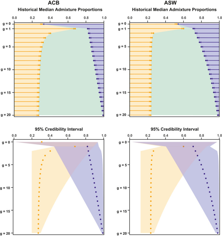
Approximate Bayesian Computation inference of the admixture history of the ACB and ASW populations respectively. Top panels are based on median point‐estimates of parameters for the relative contribution of each source to the gene pool of the admixed target population ACB and ASW, at each generation. Bottom panels show 95% credibility intervals for each inferred parameter around the median point‐estimates. The African introgression is plotted in orange, the European introgression in blue, and in green the remaining contribution of the admixed population to itself at the following generation. Left column presents results for the ACB under the AfrDE‐EurDE winning scenario; Right column presents results for the ASW under the AfrDE‐EurDE winning scenario

We found a virtual complete replacement of the ACB and ASW populations at generation 1, thus consistent with our inability to accurately estimate the founding proportions from the African and European sources at generation 0. Furthermore, we found an increasingly precise posterior estimation of introgression rates forward‐in‐time. This is also consistent with the nature of recurrent admixture processes, where older information may be lost or replaced when more recent admixture events occur.

Interestingly, we found that the recurring introgression from the European gene pool rapidly decreased after generation 1, for both the ACB and ASW, albeit with substantial differences (Figure 5). Indeed, we found that, for the ACB, European introgression falls below 10% at generation 9 to no more than 1% in the present. Comparatively, the European contribution diminished substantially less rapidly for the ASW, going below 10% only after generation 12 to roughly 2% in the present. Therefore, it seemed that neither sustained European migrations, nor the relaxation of social and legal constraints on admixture subsequent to the abolition of slavery and the end of segregation, have translated into increased European genetic contribution to the gene‐pool of admixed populations in the Americas.

Finally, we found substantial recurring contributions from the African source for both admixed populations (Figure 5). For the ACB, we found a progressive decrease of the African recurring introgression until a virtually constant recurring admixture close to 28% from generation 10 onward. For the ASW, our results showed a sharper decrease of the African contribution after founding until a virtually constant recurring admixture process close to 24% from generation 5 onward. Nevertheless, the ASW occupy an ambiguous region of the parameter space, and results should be considered cautiously, as another complex admixture model might more accurately explain this data. Altogether, the signal of substantial ongoing admixture from Africa could have emerged due to the known importance of African recurring forced migrations during the TAST into the Americas, as well as from enslaved‐African descendants migrations within the Americas before and after the end of slavery (Baharian et al., 2016; Fortes‐Lima et al., 2018).

4. DISCUSSION

Our novel methis forward‐in‐time simulator and summary statistic calculator coupled with RF‐ABC scenario‐choice could distinguish among highly complex admixture histories using genetic data. As expected, scenario‐choice errors were particularly made in regions of the parameter space for which scenarios were highly nested (Robert et al., 2010), and, thus, biologically similar. Furthermore, we found that NN‐ABC provided accurate and reasonably conservative posterior parameter estimation for numerous parameters of the winning scenario, using human population data as a case study. Finally, we empirically demonstrated that the moments of the distribution of admixture fractions in the admixed population were highly informative for ABC inference, as expected theoretically (Gravel, 2012; Verdu & Rosenberg, 2011).

In general, the machine‐learning ABC approaches here deployed for reconstructing highly complex admixture histories provided significant improvements for population genetics demographic inferences using genetic data. First, RF algorithms are, by nature, categorization algorithms and therefore a priori conceptually particularly well suited for scenario‐choice inferences as compared to, for instance, previous regression‐based ABC scenario‐choice algorithms (Beaumont et al., 2002). In addition, they substantially reduce the simulation costs while improving scenario‐choice performances, as compared to previous ABC scenario‐choice algorithms that classically require 10–100 times more simulations (Pudlo et al., 2016). Finally, RF‐ABC scenario‐choice allow exploring, in detail, the relative contribution of each summary statistic to the scenario‐choice, in addition to being insensitive to correlations among statistics. These improvements can thus both improve the user's understanding of the general behavior and performances of the scenario‐choice inference procedures applied to her/his specific study‐case, and alleviate the major difficulty induced by large spaces of summary statistics encountered in previous ABC scenario‐choice approaches (Sisson et al., 2018). Nevertheless, posterior parameter estimation with RF‐ABC remains difficult, as it only allows estimating the quantiles of the posterior parameters independently, rather than the full posterior distributions of the parameters estimated jointly (Raynal et al., 2019).

Second, NN‐ABC parameter inference also provide a promising line of future developments for posterior parameter inference based on high dimensional parameter spaces. Indeed, using NN methods allows for the joint estimation of all model parameters by weighting the informativeness of each summary statistic about the parameters, beyond what most other ABC parameter‐inference methods can do. Nevertheless, future studies will need to explore all the possibilities brought by posterior parameter inferences with NN, such as increasing the number of layers of hidden neurons, fine‐tuning the NN procedures respective to the specific weighting of each summary statistics’ importance for posterior parameter estimations, and/or different NN algorithms for exploring the space of summary statistics (Csilléry et al., 2012). These will allow researchers to fully benefit from the power of this novel conceptual way of extracting information about model parameters from population genetics statistics computed from genetic data.

Altogether, our results for the two recently‐admixed human populations illustrated how our methis‐ABC framework can bring fundamental new insights into the complex demographic history of admixed populations; a framework that can easily be adapted, using methis (Note S1), for investigating complex admixture histories when ML methods are intractable.

We considered nine competing scenarios all deriving from the general mechanistic admixture model of Verdu and Rosenberg (2011). While the two‐source version of this model can readily be simulated with methis, it considers 2g‐1 model parameters (with g the duration of the admixture process), plus effective population size parameters and mutation parameters. Estimating jointly all these parameters is out of reach of ML methods, and further probably out of reach of ABC posterior parameter estimation procedures. However, conducting ABC scenario‐choice for disentangling major classes of relatively simplified admixture processes followed by ABC parameter estimation under the winning scenario, is flexible enough to bring new insights into the evolutionary history of admixed populations, far beyond all admixture scenarios that can be explored with existing ML methods (Gravel, 2012; Hellenthal et al., 2014).

The sample and SNP set explored here is often out‐of‐reach in non‐model species. Nevertheless, our results considering vastly reduced SNP or sample sets demonstrated that ABC could remain remarkably accurate for disentangling highly complex admixture processes with much less genetic or sample data. This is due to the fact that ABC relies on the amount of information carried by summary statistics about model parameters, rather than on the absolute amount of genetic data investigated. Therefore, the methis‐ABC framework remains promising to reconstruct complex admixture histories in study‐cases with substantially fewer genetic and sample data, provided that the summary statistics considered by the user are, a priori, informative about model parameters, and that they are reasonably well estimated for the observed data. Altogether, large spaces of parameters and summary statistics, lack of information from summary statistics, and scenario nestedness, are well known to affect ABC performances and, thus, imperatively need to be thoroughly evaluated case by case (Csilléry et al., 2010; Robert et al., 2010; Sisson et al., 2018).

To further increase the range of applicability of our methis‐ABC framework, our software readily implements microsatellite markers together with a general stepwise mutation model (Estoup et al., 2002), fully parameterizable by the user (Note S1). This will allow investigating numerous complex admixture histories from non‐model species for which large amounts of SNP data are less frequently available, but for which microsatellite markers are readily available.

Even if prior knowledge of the date for the founding admixture event is lacking, methis users can simply set the founding of the admixed population in a remote past and implement a second founding event with variable date to be estimated with ABC, together with later additional admixture events and other parameters of interest. Nevertheless, it is not trivial to predict how old admixture processes can be to remain successfully investigated with ABC (Buzbas & Verdu, 2018). Indeed, ancient admixture processes could leave scarcely identifiable signatures in the observed data, if they have been obliterated by more recent admixture events. This was theoretically expected (Buzbas & Verdu, 2018), and future studies combining ancient and modern DNA samples may bring further information into the reconstruction of ancient admixture history.

Importantly, the computational cost of our study depends, for 2/3, on the calculation of all summary statistics at the end of the admixture process, as is often the case in ABC. Considering much longer admixture processes than the ones here investigated will mechanically increase computation time but will not increase summary statistics calculation time. Furthermore, note that the computational cost of simulating data with methis does not rely excessively on the number of generations considered (within reason), nor on the absolute number of markers used, but rather on the effective population size in the admixed population set by the user.

Although methis readily allows considering changes of effective population size in the admixed population at each generation as a parameter of interest to ABC inference (Note S1), we did not, for simplicity, investigate here how such changes affected our results. Future work using methis will specifically investigate how effective size changes may influence genetic patterns in admixed populations, a question of major interest as numerous admixed populations have experienced bottlenecks during their genetic history (e.g., Browning et al., 2018).

The current methis‐ABC approach does not make use of admixture linkage‐disequilibrium patterns in the admixed population, and only relies on independent SNP or microsatellite markers. Nevertheless, admixture‐LD has consistently proved to bring massive information about complex admixture histories in populations where large genomic data sets were available (Gravel, 2012; Hellenthal et al., 2014; Malinsky et al., 2018; Medina et al., 2018; Ni et al., 2019; Stryjewski & Sorenson, 2017). However, existing methods to calculate admixture‐LD patterns remain computationally intensive and require both dense marker‐sets and accurate phasing, which is difficult under ABC where such statistics have to be calculated for each one of the numerous simulated data sets. In this context, RF‐ABC (Pudlo et al., 2016; Raynal et al., 2019), or AABC (Buzbas & Rosenberg, 2015), methods substantially reduce the number of simulations required for satisfactory ABC inference. This makes both approaches promising for using, in the future, admixture‐LD patterns to reconstruct complex admixture processes with ABC using genomic data.

Finally, future developments of the methis‐ABC framework will focus on implementing sex‐specific admixture models, as these processes are known to affect genetic diversity patterns in a specific way, and are of interest to numerous study‐cases (Goldberg et al., 2014). Furthermore, the methis forward‐in‐time simulator represents an ideal tool to further investigate admixture‐related selection forces, and admixture‐specific assortative mating processes, as these processes can simply be modeled by specifically parameterizing individual reproduction and survival in the simulations, unlike most coalescent‐based simulators.

AUTHOR CONTRIBUTIONS

Cesar A. Fortes‐Lima built the alpha version of the software, conducted preliminary benchmarking and data analyses, and assisted in writing the article. Romain Laurent built the beta version of the software, conducted benchmarking and data analyses and assisted in writing the article. Valentin Thouzeau conducted benchmarking and data analyses and assisted in writing the article. Bruno Toupance assisted in building the beta version of the software, conducted benchmarking and data analyses and assisted in writing the article. Paul Verdu designed and supervised the project, conducted benchmarking and data analyses and wrote the article.

Supporting information

Supplementary Material

Note S1

Note S2

DATA AVAILABILITY STATEMENT

methis software package is open source under the GNU General Public License v3.0, and can be downloaded with manual and example data sets from https://github.com/romain‐laurent/MetHis. Genetic data used in this article were downloaded from the 1000 Genome Project Phase 3 open‐access data repository (https://www.internationalgenome.org/data/).

REFERENCES

- Alexander, D. H. , Novembre, J. , & Lange, K. (2009). Fast model‐based estimation of ancestry in unrelated individuals. Genome Research, 19(9), 1655–1664. 10.1101/gr.094052.109. [DOI] [PMC free article] [PubMed] [Google Scholar]
- Baharian, S. , Barakatt, M. , Gignoux, C. R. , Shringarpure, S. , Errington, J. , Blot, W. J. , Bustamante, C. D. , Kenny, E. E. , Williams, S. M. , Aldrich, M. C. , & Gravel, S. (2016). The great migration and African‐American genomic diversity. PLoS Genetics, 12(5), e1006059. 10.1371/journal.pgen.1006059. [DOI] [PMC free article] [PubMed] [Google Scholar]
- Beaumont, M. A. , Zhang, W. , & Balding, D. J. (2002). Approximate Bayesian computation in population genetics. Genetics, 162(4), 2025–2035. [DOI] [PMC free article] [PubMed] [Google Scholar]
- Bernstein, F. (1931). Die geographische Verteilung der Bludgruppen und ihre anthropologische Bedeutung. In Comitato Italiano per o studio dei problemi della populazione (pp. 227–243). : Instituto Poligraphico dello Stato. [Google Scholar]
- Blum, M. G. B. , & François, O. (2010). Non‐linear regression models for Approximate Bayesian Computation. Statistics and Computing, 20, 63–67. 10.1007/s11222-009-9116-0. [DOI] [Google Scholar]
- Boitard, S. , Rodriguez, W. , Jay, F. , Mona, S. , & Austerlitz, F. (2016). Inferring population size history from large samples of genome‐wide molecular data ‐ An approximate bayesian computation approach. PLoS Genetics, 12(3), e1005877. 10.1371/journal.pgen.1005877. [DOI] [PMC free article] [PubMed] [Google Scholar]
- Bowcock, A. M. , Ruiz‐Linares, A. , Tomfohrde, J. , Minch, E. , Kidd, J. R. , & Cavalli‐Sforza, L. L. (1994). High resolution of human evolutionary trees with polymorphic microsatellites. Nature, 368(6470), 455–457. 10.1038/368455a0. [DOI] [PubMed] [Google Scholar]
- Brandenburg, J.‐T. , Mary‐Huard, T. , Rigaill, G. , Hearne, S. J. , Corti, H. , Joets, J. , Vitte, C. , Charcosset, A. , Nicolas, S. D. , & Tenaillon, M. I. (2017). Independent introductions and admixtures have contributed to adaptation of European maize and its American counterparts. PLOS Genetics, 13(3), e1006666. 10.1371/journal.pgen.1006666. [DOI] [PMC free article] [PubMed] [Google Scholar]
- Browning, S. R. , Browning, B. L. , Daviglus, M. L. , Durazo‐Arvizu, R. A. , Schneiderman, N. , Kaplan, R. C. , & Laurie, C. C. (2018). Ancestry‐specific recent effective population size in the Americas. PLoS Genetics, 14(5), e1007385. 10.1371/journal.pgen.1007385. [DOI] [PMC free article] [PubMed] [Google Scholar]
- Buzbas, E. O. , & Rosenberg, N. A. (2015). AABC: approximate approximate Bayesian computation for inference in population‐genetic models. Theoretical Population Biology, 99, 31–42. 10.1016/j.tpb.2014.09.002. [DOI] [PMC free article] [PubMed] [Google Scholar]
- Buzbas, E. O. , & Verdu, P. (2018). Inference on admixture fractions in a mechanistic model of recurrent admixture. Theoretical Population Biology, 122, 149–157. 10.1016/j.tpb.2018.03.006. [DOI] [PMC free article] [PubMed] [Google Scholar]
- Cavalli‐Sforza, L. L. , & Bodmer, W. F. (1971). The genetics of human populations. W. H. Freeman. [Google Scholar]
- Chakraborty, R. , & Weiss, K. M. (1988). Admixture as a tool for finding linked genes and detecting that difference from allelic association between loci. Proceedings of the National Academy of Sciences of the United States of America, 85(23), 9119–9123. [DOI] [PMC free article] [PubMed] [Google Scholar]
- Chimusa, E. R. , Defo, J. , Thami, P. K. , Awany, D. , Mulisa, D. D. , Allali, I. , Ghazal, H. , Moussa, A. , & Mazandu, G. K. (2018). Dating admixture events is unsolved problem in multi‐way admixed populations. Briefings in Bioinformatics, 144–155. 10.1093/bib/bby112. [DOI] [PMC free article] [PubMed] [Google Scholar]
- Csilléry, K. , Blum, M. G. , Gaggiotti, O. E. , & Francois, O. (2010). Approximate Bayesian Computation (ABC) in practice. Trends in Ecology and Evolution, 25(7), 410–418. 10.1016/j.tree.2010.04.001. [DOI] [PubMed] [Google Scholar]
- Csilléry, K. , François, O. , & Blum, M. G. B. (2012). abc: an R package for approximate Bayesian computation (ABC). Methods in Ecology and Evolution, 3, 475–479. [DOI] [PubMed] [Google Scholar]
- Epstein Michael P., Duren William L., Boehnke M. (2000). Improved Inference of Relationship for Pairs of Individuals. The American Journal of Human Genetics, 67(5), 1219–1231. 10.1016/s0002-9297(07)62952-8. [DOI] [PMC free article] [PubMed] [Google Scholar]
- Estoup, A. , Jarne, P. , & Cornuet, J. M. (2002). Homoplasy and mutation model at microsatellite loci and their consequences for population genetics analysis. Molecular Ecology, 11, 1591–1604. [DOI] [PubMed] [Google Scholar]
- Estoup, A. , Raynal, L. , Verdu, P. , & Marin, J. M. (2018). Model choice using Approximate Bayesian Computation and Random Forests: analyses based on model grouping to make inferences about the genetic history of Pygmy human populations. Journal of the SFdS, 159(3), 167–190. [Google Scholar]
- Excoffier, L. , Dupanloup, I. , Huerta‐Sanchez, E. , Sousa, V. C. , & Foll, M. (2013). Robust demographic inference from genomic and SNP data. PLOS Genetics, 9(10), e1003905. 10.1371/journal.pgen.1003905. [DOI] [PMC free article] [PubMed] [Google Scholar]
- Excoffier, L. , & Foll, M. (2011). fastsimcoal: a continuous‐time coalescent simulator of genomic diversity under arbitrarily complex evolutionary scenarios. Bioinformatics, 27(9), 1332–1334. 10.1093/bioinformatics/btr124. [DOI] [PubMed] [Google Scholar]
- Falush, D. , Stephens, M. , & Pritchard, J. K. (2003). Inference of population structure using multilocus genotype data: linked loci and correlated allele frequencies. Genetics, 164(4), 1567–1587. [DOI] [PMC free article] [PubMed] [Google Scholar]
- Fisher, R. A. (1922). Darwinian evolution of mutations. Eugenics Review, 14(1), 31–34. [PMC free article] [PubMed] [Google Scholar]
- Foll, M. , Shim, H. , & Jensen, J. D. (2015). WFABC: a Wright‐Fisher ABC‐based approach for inferring effective population sizes and selection coefficients from time‐sampled data. Molecular Ecology Resources, 15(1), 87–98. 10.1111/1755-0998.12280. [DOI] [PubMed] [Google Scholar]
- Fortes‐Lima, C. , Bybjerg‐Grauholm, J. , Marin‐Padrón, L. C. , Gomez‐Cabezas, E. J. , Bækvad‐Hansen, M. , Hansen, C. S. , Le, P. , Hougaard, D. M. , Verdu, P. , Mors, O. , Parra, E. J. , & Marcheco‐Teruel, B. (2018). Exploring Cuba’s population structure and demographic history using genome‐wide data. Scientific Reports, 8(1), 11422. 10.1038/s41598-018-29851-3. [DOI] [PMC free article] [PubMed] [Google Scholar]
- Fraimout, A. , Debat, V. , Fellous, S. , Hufbauer, R. A. , Foucaud, J. , Pudlo, P. , & Estoup, A. (2017). Deciphering the routes of invasion of Drosophila suzukii by means of ABC random forest. Molecular Biology and Evolution, 34(4), 980–996. 10.1093/molbev/msx050. [DOI] [PMC free article] [PubMed] [Google Scholar]
- Genomes Project Consortium (2015). A global reference for human genetic variation. Nature, 526(7571), 68–74. 10.1038/nature15393. [DOI] [PMC free article] [PubMed] [Google Scholar]
- Goldberg, A. , Verdu, P. , & Rosenberg, N. A. (2014). Autosomal admixture levels are informative about sex bias in admixed populations. Genetics, 198(3), 1209–1229. [DOI] [PMC free article] [PubMed] [Google Scholar]
- Gravel, S. (2012). Population genetics models of local ancestry. Genetics, 191(2), 607–619. 10.1534/genetics.112.139808. [DOI] [PMC free article] [PubMed] [Google Scholar]
- Guan, Y. (2014). Detecting structure of haplotypes and local ancestry. Genetics, 196(3), 625–642. 10.1534/genetics.113.160697. [DOI] [PMC free article] [PubMed] [Google Scholar]
- Hellenthal, G. , Busby, G. B. J. , Band, G. , Wilson, J. F. , Capelli, C. , Falush, D. , & Myers, S. (2014). A genetic atlas of human admixture history. Science, 343(6172), 747–751. 10.1126/science.1243518. [DOI] [PMC free article] [PubMed] [Google Scholar]
- Jay, F. , Boitard, S. , & Austerlitz, F. (2019). An ABC method for whole‐genome sequence data: Inferring paleolithic and neolithic human expansions. Molecular Biology and Evolution, 36(7), 1565–1579. 10.1093/molbev/msz038. [DOI] [PubMed] [Google Scholar]
- Lipson, M. , Loh, P. R. , Levin, A. , Reich, D. , Patterson, N. , & Berger, B. (2013). Efficient moment‐based inference of admixture parameters and sources of gene flow. Molecular Biology and Evolution, 30(8), 1788–1802. 10.1093/molbev/mst099. [DOI] [PMC free article] [PubMed] [Google Scholar]
- Loh, P. R. , Lipson, M. , Patterson, N. , Moorjani, P. , Pickrell, J. K. , Reich, D. , & Berger, B. (2013). Inferring admixture histories of human populations using linkage disequilibrium. Genetics, 193(4), 1233–1254. 10.1534/genetics.112.147330. [DOI] [PMC free article] [PubMed] [Google Scholar]
- Long, J. C. (1991). The genetic structure of admixed populations. Genetics, 127(2), 417–428. [DOI] [PMC free article] [PubMed] [Google Scholar]
- Malinsky, M. , Trucchi, E. , Lawson, D. J. , & Falush, D. (2018). RADpainter and fineRADstructure: Population Inference from RADseq Data. Molecular Biology and Evolution, 35(5), 1284–1290. 10.1093/molbev/msy023. [DOI] [PMC free article] [PubMed] [Google Scholar]
- Martin, A. R. , Gignoux, C. R. , Walters, R. K. , Wojcik, G. L. , Neale, B. M. , Gravel, S. , Daly, M. J. , Bustamante, C. D. , & Kenny, E. E. (2017). Human demographic history impacts genetic risk prediction across diverse populations. American Journal of Human Genetics, 100(4), 635–649. 10.1016/j.ajhg.2017.03.004. [DOI] [PMC free article] [PubMed] [Google Scholar]
- Martin, S. H. , Dasmahapatra, K. K. , Nadeau, N. J. , Salazar, C. , Walters, J. R. , Simpson, F. , & Jiggins, C. D. (2013). Genome‐wide evidence for speciation with gene flow in Heliconius butterflies. Genome Research, 23(11), 1817–1828. 10.1101/gr.159426.113. [DOI] [PMC free article] [PubMed] [Google Scholar]
- Medina, P. , Thornlow, B. , Nielsen, R. , & Corbett‐Detig, R. (2018). Estimating the timing of multiple admixture pulses during local ancestry inference. Genetics, 210(3), 1089–1107. 10.1534/genetics.118.301411. [DOI] [PMC free article] [PubMed] [Google Scholar]
- Moorjani, P. , Patterson, N. , Hirschhorn, J. N. , Keinan, A. , Hao, L. I. , Atzmon, G. , Burns, E. , Ostrer, H. , Price, A. L. , & Reich, D. (2011). The history of African gene flow into Southern Europeans, Levantines, and Jews. PLOS Genetics, 7(4), e1001373. 10.1371/journal.pgen.1001373. [DOI] [PMC free article] [PubMed] [Google Scholar]
- Nei, M. (1978). Estimation of average heterozygosity and genetic distance from a small number of individuals. Genetics, 89(3), 583–590. [DOI] [PMC free article] [PubMed] [Google Scholar]
- Ni, X. , Yuan, K. , Liu, C. , Feng, Q. , Tian, L. , Ma, Z. , & Xu, S. (2019). MultiWaver 2.0: modeling discrete and continuous gene flow to reconstruct complex population admixtures. European Journal of Human Genetics, 27(1), 133–139. 10.1038/s41431-018-0259-3. [DOI] [PMC free article] [PubMed] [Google Scholar]
- Patin, E. , Lopez, M. , Grollemund, R. , Verdu, P. , Harmant, C. , Quach, H. , Laval, G. , Perry, G. H. , Barreiro, L. B. , Froment, A. , Heyer, E. , Massougbodji, A. , Fortes‐Lima, C. , Migot‐Nabias, F. , Bellis, G. , Dugoujon, J.‐M. , Pereira, J. B. , Fernandes, V. , Pereira, L. , … Quintana‐Murci, L. (2017). Dispersals and genetic adaptation of Bantu‐speaking populations in Africa and North America. Science, 356(6337), 543–546. 10.1126/science.aal1988. [DOI] [PubMed] [Google Scholar]
- Patterson, N. , Moorjani, P. , Luo, Y. , Mallick, S. , Rohland, N. , Zhan, Y. , Genschoreck, T. , Webster, T. , & Reich, D. (2012). Ancient admixture in human history. Genetics, 192(3), 1065–1093. 10.1534/genetics.112.145037. [DOI] [PMC free article] [PubMed] [Google Scholar]
- Pickrell, J. K. , & Pritchard, J. K. (2012). Inference of population splits and mixtures from genome‐wide allele frequency data. PLOS Genetics, 8(11), e1002967. 10.1371/journal.pgen.1002967. [DOI] [PMC free article] [PubMed] [Google Scholar]
- Pritchard, J. K. , Seielstad, M. T. , Perez‐Lezaun, A. , & Feldman, M. W. (1999). Population growth of human Y chromosomes: a study of Y chromosome microsatellites. Molecular Biology and Evolution, 16(12), 1791–1798. 10.1093/oxfordjournals.molbev.a026091. [DOI] [PubMed] [Google Scholar]
- Pudlo, P. , Marin, J. M. , Estoup, A. , Cornuet, J. M. , Gautier, M. , & Robert, C. P. (2016). Reliable ABC model choice via random forests. Bioinformatics, 32(6), 859–866. 10.1093/bioinformatics/btv684. [DOI] [PubMed] [Google Scholar]
- Purcell S., Neale B., Todd‐Brown K., Thomas L., Ferreira M. A. R., Bender D., Maller J., Sklar P., de Bakker P. I. W., Daly M. J., Sham P. C. (2007). PLINK: A Tool Set for Whole‐Genome Association and Population‐Based Linkage Analyses. The American Journal of Human Genetics, 81(3), 559–575. 10.1086/519795. [DOI] [PMC free article] [PubMed] [Google Scholar]
- R Development Core Team (2020). R: A language and environment for statistical computing. R Foundation for Statistical Computing. Retrieved from http://www.R‐project.org. [Google Scholar]
- Raynal, L. , Marin, J. M. , Pudlo, P. , Ribatet, M. , Robert, C. P. , & Estoup, A. (2019). ABC random forests for Bayesian parameter inference. Bioinformatics, 35(10), 1720–1728. 10.1093/bioinformatics/bty867. [DOI] [PubMed] [Google Scholar]
- Robert, C. P. , Mengersen, K. , & Chen, C. (2010). Model choice versus model criticism. Proceedings of the National Academy of Sciences, 107(3), E5–E5. 10.1073/pnas.0911260107. [DOI] [PMC free article] [PubMed] [Google Scholar]
- Sisson, S. A. , Fan, Y. , & Beaumont, M. A. (2018). In Sisson S. A., Fan Y., & Beaumont M. A. (Eds.). Handbook of approximate bayesian computation. pp 678. New York, NY: Chapman and Hall/CRC. [Google Scholar]
- Skoglund, P. , Ersmark, E. , Palkopoulou, E. , & Dalen, L. (2015). Ancient wolf genome reveals an early divergence of domestic dog ancestors and admixture into high‐latitude breeds. Current Biology, 25(11), 1515–1519. 10.1016/j.cub.2015.04.019. [DOI] [PubMed] [Google Scholar]
- Stryjewski, K. F. , & Sorenson, M. D. (2017). Mosaic genome evolution in a recent and rapid avian radiation. Nature Ecology and Evolution, 1(12), 1912–1922. 10.1038/s41559-017-0364-7. [DOI] [PubMed] [Google Scholar]
- Tavaré, S. , Balding, D. J. , Griffiths, R. C. , & Donnelly, P. (1997). Inferring coalescence times from DNA sequence data. Genetics, 145(2), 505–518. [DOI] [PMC free article] [PubMed] [Google Scholar]
- Verdu, P. , Austerlitz, F. , Estoup, A. , Vitalis, R. , Georges, M. , Théry, S. , Froment, A. , Le Bomin, S. , Gessain, A. , Hombert, J.‐M. , Van der Veen, L. , Quintana‐Murci, L. , Bahuchet, S. , & Heyer, E. (2009). Origins and genetic diversity of pygmy hunter‐gatherers from Western Central Africa. Current Biology, 19(4), 312–318. 10.1016/j.cub.2008.12.049. [DOI] [PubMed] [Google Scholar]
- Verdu, P. , Jewett, E. M. , Pemberton, T. J. , Rosenberg, N. A. , & Baptista, M. (2017). Parallel trajectories of genetic and linguistic admixture in a genetically admixed creole population. Current Biology, 27(16), 2529–2535 e2523. 10.1016/j.cub.2017.07.002. [DOI] [PubMed] [Google Scholar]
- Verdu, P. , & Rosenberg, N. A. (2011). A general mechanistic model for admixture histories of hybrid populations. Genetics, 189(4), 1413–1426. 10.1534/genetics.111.132787. [DOI] [PMC free article] [PubMed] [Google Scholar]
- Wakeley, J. , King, L. , Low, B. S. , & Ramachandran, S. (2012). Gene genealogies within a fixed pedigree, and the robustness of Kingman's coalescent. Genetics, 190(4), 1433–1445. 10.1534/genetics.111.135574. [DOI] [PMC free article] [PubMed] [Google Scholar]
- Wegmann, D. , Leuenberger, C. , & Excoffier, L. (2009). Efficient approximate Bayesian computation coupled with Markov chain Monte Carlo without likelihood. Genetics, 182(4), 1207–1218. 10.1534/genetics.109.102509. [DOI] [PMC free article] [PubMed] [Google Scholar]
- Weir, B. S. , & Cockerham, C. C. (1984). Estimating F‐statistics for the analysis of population‐structure. Evolution, 38(6), 1358–1370. [DOI] [PubMed] [Google Scholar]
- Wright, S. (1931). Evolution in Mendelian populations. Genetics, 16(2), 97–159. [DOI] [PMC free article] [PubMed] [Google Scholar]
Associated Data
This section collects any data citations, data availability statements, or supplementary materials included in this article.
Supplementary Materials