Variable selection with Group LASSO approach: Application to Cox regression with frailty model

Abstract

In analysis of survival outcomes supplemented with both clinical information and high-dimensional gene expression data, use of the traditional Cox proportional hazards model fails to meet some emerging needs in biomedical research. First, the number of covariates is generally much larger the sample size. Secondly, predicting an outcome based on individual gene expression is inadequate because multiple biological processes and functional pathways regulate phenotypic expression. Another challenge is that the Cox model assumes that populations are homogenous, implying that all individuals have the same risk of death, which is rarely true due to unmeasured risk factors among populations. In this paper we propose group LASSO with gamma-distributed frailty for variable selection in Cox regression by extending previous scholarship to account for heterogeneity among group structures related to exposure and susceptibility. The consistency property of the proposed method is established. This method is appropriate for addressing a wide variety of research questions from genetics to air pollution. Simulated and real world data analysis shows promising performance by group LASSO compared with other methods, including group SCAD and group MCP. Future research directions include expanding the use of frailty with adaptive group LASSO and sparse group LASSO methods.

1. Introduction

1.1. Survival Analysis

Survival analysis models the time it takes for death and other long-term events to occur, focusing on the distribution of survival times. Survival modeling examines the relationship between survival and one or more predictors, usually called covariates. The semi-parametric approach is one of three approaches found in survival analysis, which assumes that the real probability distributions of observations belong to a class of laws dependent upon parameters, while other parts are written as non-parametric functions (Cox 1972; Cox & Oakes 1984).

Cox regression models the impact of predictors on the hazard function, which characterizes for an individual j the probability of dying or experiencing a particular outcome within a short interval of time provided the individual has survived or not experienced the outcome previously. Many extended versions of the Cox regression model have been implemented to take into account clustered data or groups within which the failure times may be correlated (Martinussen & Scheike 2006). These groups may represent such distinct entities as members of the same family, patients in the same hospital, or organs within an individual. Grouping structures arise naturally in many statistical modeling problems. As addressed by (Ma et al. 2007), complex diseases such as cancer are often caused by mutations in pathways involving multiple genes; therefore, it is preferable to select groups of related genes together rather than individual genes separately if they operate on the same causal pathway.

In linear regression, variable selection techniques such as best subset and forward and backward stepwise selection have traditionally been used. However, these types of approaches are often unsatisfactory for reasons related to problems with high-dimensional data and computational intensity (Breiman 1995; Fani & Li 2001, Greenland 2008, Hastie et al. 2009). Penalized regression techniques have been proposed to accomplish the same goals as these techniques but in a more stable, continuous, and computationally efficient fashion. These techniques include a L₁ absolute value “Least Absolute Shrinkage and Selection Operator” (“LASSO”) penalty (Tibshirani 1996, 1997), and a L₂ quadratic (“ridge”) penalty (Hoerl & Kennard 1970; Le Cessie & van Houwelingen 1992; Verweij & Van Houwelingen 1994).

L₁ and L₂ penalized estimation methods shrink the estimates of the regression coefficients towards zero relative to the maximum likelihood estimates. The purpose of this shrinkage is to prevent overfitting due to either collinearity of the covariates or high dimensionality but can suffer poor performance with some highly correlated datasets (Hou et al. 2018). Although both methods are shrinkage oriented, the effects of L₁ and L₂ penalization are quite different in practice. Applying a L₂ penalty tends to result in all small but non-zero regression coefficients. As a continuous shrinkage method, if there is high correlation between predictors, ridge regression achieves better predictive performance through a bias-variance trade-off that favors ridge over LASSO (Tibshirani 1996). However, ridge regression cannot produce a parsimonious model, as it produces coefficient values for each of the predictor variables. Applying a L₁ penalty tends to result in many regression coefficients shrunk to zero and a few other regression coefficients with comparatively little shrinkage. Consequently, LASSO is popular due to its sparse output. The L₁ penalty has been applied to other models including Cox regression (Tibshirani 1997) and logistic regression (Lokhorst 1999; Roth 2004; Genkin et al. 2007).

1.2. Literature review and problem statement

This method is an extension of the popular model selection and shrinkage estimation L₁ penalty technique to address the problem of variable selection in high dimensions (i.e., the number of regressors p is greater than the number of observations n). Group LASSO (Bakin 1999; Cai 2001, Antoniadis & Fan 2001; Youan & Lin 2006 Meier et al. 2008) handles these problems by extending the LASSO penalty to cover group variable structures and has been applied to survival analysis (Kim et al. 2012).

Estimating coefficients in group LASSO is slightly different from standard LASSO because the constraints are now applied to each grouping of variables. In regular LASSO it is possible to have a different constraint for each coefficient. Group LASSO removes a set of explanatory variables in the model by shrinking its corresponding parameter to zero and keeping a subset of significant variables upon which the hazard function depends. Some tuning parameter λ is used for each factor without assessing its relative importance. It has been shown that such an excessive penalty applied to the relevant variables can degrade the estimation efficiency (Fan & Li 2001) and affect the selection consistency (Leng et al. 2006; Yuan & Lin 2006; Zou 2006). Group LASSO suffers the same drawback; to address this issue, Wang & Leng (2008) proposed adaptive group LASSO, which allows for unique tuning parameter values to be used for different factors. Such flexibility in turn produces variable amounts of shrinkage for different factors.

In the classic semi-parametric Cox model, the study population is implicitly assumed to be homogeneous, meaning all individuals have the same risk of death. This assumption rarely holds true. Individuals within a group may possess a non-observed susceptibility to death from differential genetic predisposition to certain diseases or have common environmental exposures that influence time to the studied event (Gilhodes et al. 2017). Another assumption in survival analysis is that individuals under observation are independent; however, individuals of the same group may share unobserved risk factors. Typical groups sharing risk factors include families, villages, hospitals, and repeated measurements on one individual (Fu et al. 2017). A simple model for dependent survival times that is a generalization of the proportional hazard model can be implemented using the concept of frailty. This was first proposed by Vaupel et al. (1979).

The frailty distributions that have been studied mostly belong to the power variance function family, a particular set of distributions introduced first by Tweedy (1984) and later independently studied by Hougaard (1986). The gamma, inverse Gaussian, positive stable, and compound Poisson distributions are all members of this group. Generally, the gamma distribution is used to model frailty for sake of mathematical convenience. It has been demonstrated that its Laplace transform is a useful mathematical tool for several measures of dependence, and the n^th derivative of its Laplace transform has a simple notation. To control the hidden heterogeneity and/or dependence among individuals with a group-related “frailty,” we introduce into our model a random variable that follows a gamma distribution. In frailty modeling, the gamma distribution is typically parametrized with one parameter being used simultaneously for both shape and scale.

Fan & Li (2002) proposed LASSO for the Cox proportional hazard frailty model. In this paper, we further improve this procedure by extending it to group LASSO for the Cox proportional hazard frailty model for survival censored times in high dimensions. This method takes into account group structure and linkages between predictor variables that are supplied in the model. Additionally, allowance is made for a group-level frailty related to unmeasured but suspected background vulnerability or resilience to a particular disease outcome. This model algorithm, using group LASSO with the Cox proportional hazard frailty model, is most applicable in situations with the aforementioned individual and outcome characteristics. In this paper, this method is demonstrated with both simulated and real datasets.

Section 2 describes the model and the necessary mathematical underpinnings for the following parts. Section 3 builds on the previous section and describes the algorithm for choosing model parameters β. Section 4 gives details proving theoretical consistency of the method. Section 5 describes applications of this modeling method, and Section 6 gives examples of these using simulated and true datasets. Section 7 concludes with a brief discussion of the results, limitations, and futures uses of the method.

2. Methods

2.1. Model set-up

Suppose that there are n clusters and that the i^th cluster has J_i individuals with unobserved shared frailty u_i(1 ≤ i ≤ n). A vector X_ij(1 ≤ i ≤ n, 1 ≤ j ≤ J_i) is associated with the ij^th survival time T_ij of the j^th individual in the i^th cluster. Assume that we have independent and identically distributed survival data for a subject j in i^th cluster: (Z_ij, δ_ij, X_ij, u_i) with ${\delta }_{ij}={\mathbb{1}}_{\left\{T_{ij}\le C_{ij}\right\}}$ the status indicator of censoring, C_ij the censoring time and Z_ij = min(T_ij, C_ij) the observed time for individual j of cluster i. The corresponding likelihood function with a shared gamma frailty is given by

$$L_n\left(\beta ,\alpha ,H_0(.)\right)=\prod _{i=1}^n\prod _{j=1}^{J_i}\left\{h_{ij}{\left(Z_{ij}\backslash u_i,X_{ij}\right)}^{{\delta }_{ij}}{S}_{ij}\left(Z_{ij}\backslash u_i,X_{ij}\right)\right\}\prod _{i=1}^{n}g\left(u_i\right)$$ (2.1)

where S(t) = exp(−H₀(t)) refers to a conditional survival function and h(t \ X, u) a conditional hazard function of T given X and u with the $u_i^{\prime }s$ representing group-level frailties. Let the frailty have a gamma distribution with the density of u written as:

$$g(u)=\frac{{\alpha }^{\alpha }{u}^{\alpha -1}\exp (-\alpha u)}{\mathrm{\Gamma }(\alpha )}$$

Consider the Cox proportional hazard with frailty model,

$$h_{ij}\left(t\backslash X_{ij},u_i\right)=h_o(t)u_i\exp \left({\beta }^{\top }{X}_{ij}\right)$$ (2.2)

with h₀(t) the baseline hazard function and β the parameter vector of interest, where $H_0(t)={\int }_0^t{h}_o(\mu )d\mu$ is the cumulative baseline hazard function. From (2.1) the likelihood becomes

$$L_n\left(\beta ,\alpha ,H_0(.)\right)=\prod _{i=1}^n\prod _{j=1}^{J_i}{h}_0{\left(Z_{ij}\right)}^{{\delta }_{ij}}\exp \left({\beta }^{\top }{X}_{ij}\right)u_i^{{\delta }_{ij}}\exp \left\{-H_0\left(Z_{ij}\right)\exp \left({\beta }^{\top }{X}_{ij}\right)u_i\right\}\prod _{i=1}^{n}g\left(u_i\right).$$ (2.3)

The likelihood of the observed data, after integration of the expression (2.3) with respect to u₁, …, u_n, is given by

$$\begin{gathered} {\int }_{u_1}\cdots {\int }_{u_n}\prod _{i=1}^n\prod _{j=1}^{J_i}\left\{h_0{\left(Z_{ij}\right)}^{{\delta }_{ij}}\exp \left({\beta }^{\top }{X}_{ij}\right)u_i^{{\delta }_{ij}}\exp \left[-H_0\left(Z_{ij}\right)\exp \left({\beta }^{\top }{X}_{ij}\right)u_i\right]\right\}\prod _{i=1}^{n}g\left(u_i\right)d{u}_n\dots d{u}_1 \\ =\prod _{i=1}^n\prod _{j=1}^{J_i}{h}_0{\left(Z_{ij}\right)}^{{\delta }_{ij}}\exp \left({\beta }^{\top }{X}_{ij}\right) \\ \times \underbrace{{\int }_{u_1}\dots {\int }_{u_n}\prod _{i=1}^n\left\{\prod _{j=1}^{J_i}{u}_i^{{\delta }_{ij}}\exp \left[-H_0\left(Z_{ij}\right)\exp \left({\beta }^{\top }{X}_{ij}\right)u_i\right]\right\}\prod _{i=1}^{n}g\left(u_i\right)d{u}_n\dots d{u}_1}. \end{gathered}$$

Let’s set A equal to the last term.

$$\begin{gathered} A={\int }_{u_1}\dots {\int }_{u_n}\prod _{i=1}^n\left\{\prod _{j=1}^{J_i}{u}_i^{{\delta }_i{}_j}\exp \left[-H_0\left(Z_{ij}\right)\exp \left({\beta }^{\top }{X}_{ij}\right)u_i\right]\right\}\prod _{i=1}^{n}g\left(u_i\right)d{u}_n\dots d{u}_1. \\ ={\int }_{u_1}\dots {\int }_{u_n}\prod _{i=1}^n\left\{u_i^{{\sum }_{j=1}^{J_i}{\delta }_{ij}}\exp \left[-\sum _{j=1}^{J_i}{H}_0\left(Z_{ij}\right)\exp \left({\beta }^{\top }{X}_{ij}\right)u_i\right]g\left(u_i\right)\right\}d{u}_n\dots d{u}_1 \end{gathered}$$ (2.4)

$$A=\prod _{i=1}^n\underbrace{{\int }_{u_i}{u}_i^{\left(A_i+\alpha \right)-1}\exp \left\{-\left[\sum _{j=1}^{J_i}{H}_0\left(Z_{ij}\right)\exp \left({\beta }^{\top }{X}_{ij}\right)+\alpha \right]u_i\right\}d{u}_i}\times \prod _{i=1}^n\frac{{\alpha }^{\alpha }}{\mathrm{\Gamma }(\alpha )}$$ (2.5)

where $A_i={\sum }_{j=1}^{J_i}{\delta }_{ij}$.

Considering the following variable substitution $k=\left[{\sum }_{j=1}^{J_i}{H}_0\left(Z_{ij}\right)\exp \left({\beta }^{\top }{X}_{ij}\right)+\alpha \right]$, then

$$\begin{gathered} A=\prod _{i=1}^n{\int }_{u_i}{\left(k{u}_i\right)}^{\left(A_i+\alpha \right)-1}\exp \left(-\left(k{u}_i\right)\right)d\left(k{u}_i\right)\frac{1}{{(k)}^{A_i+\alpha }}\prod _{i=1}^n\frac{{\alpha }^{\alpha }}{\mathrm{\Gamma }(\alpha )} \\ A=\prod _{i=1}^n\mathrm{\Gamma }\left(A_i+\alpha \right)\frac{1}{{\left[{\sum }_{j=1}^{J_i}{H}_0\left(Z_{ij}\right)\exp \left({\beta }^{\top }{X}_{ij}\right)+\alpha \right]}^{A_i+\alpha }}\prod _{i=1}^n\frac{{\alpha }^{\alpha }}{\mathrm{\Gamma }(\alpha )} \end{gathered}$$

We can deduce the likelihood of the observed data as

$$L_n\left(\beta ,\alpha ,H_0(.)\right)=\prod _{i=1}^n\frac{{\alpha }^{\alpha }{\prod }_{j=1}^{J_i}{h}_0{\left(Z_{ij}\right)}^{{\delta }_{ij}}\exp \left({\beta }^{\top }{X}_{ij}\right){\delta }_{ij}}{\mathrm{\Gamma }(\alpha ){\left[{\sum }_{j=1}^{J_i}{H}_0\left(Z_{ij}\right)\exp \left({\beta }^{\top }{X}_{ij}\right)+\alpha \right]}^{A_i+\alpha }}\mathrm{\Gamma }\left(A_i+\alpha \right)$$ (2.6)

Therefore, the log-likelihood in (2.6) is given by

$$\begin{gathered} {\ell }_n\left(\beta ,\alpha ,H_0(.)\right)=\sum _{i=1}^n\{\alpha \log \alpha +\sum _{j=1}^{J_i}[{\beta }^{\top }{X}_{ij}{\delta }_{ij}+{\delta }_{ij}\log h_0(Z_{ij})]+\log \mathrm{\Gamma }(A_i+\alpha )-\log \mathrm{\Gamma }(\alpha ) \\ -(A_i+\alpha )\log [\sum _{j=1}^{J_i}{H}_0(Z_{ij})\exp {\beta }^{\top }{X}_{ij})+\alpha ]\} \end{gathered}$$ (2.7)

We formulate a profiled likelihood as follows: Consider the least informative nonparametric model for H₀(.) in which H₀(Z_ij) has a possible jump of size ρ_l at the observed failure time ${\tilde{Z}}_l$. Then

$$\begin{gathered} H_0\left(Z_{ij}\right)=\sum _{l=1}^N{\rho }_l{\mathbb{1}}_{\left\{{\tilde{Z}}_l\le Z_{ij}\right\}} \\ {h}_0\left(Z_{ij}\right)=\prod _{l=1}^N{\rho }_l^{{\mathbb{1}}_{\{{\overline{Z}}_l\le Z_{ij}\}}} \end{gathered}$$ (2.8)

where ${\tilde{Z}}_l$, l = 1, …, N are pooled observed failure times.

Substituting (2.8) in (2.7) and differentiating with respect to ρ_k, we get

$$\begin{gathered} \frac{\partial {\ell }_n\left(\beta ,\alpha ,H_0(.)\right)}{\partial {\rho }_k}=\sum _{i=1}^n\sum _{j=1}^{J_i}{\delta }_{ij}{\mathbb{1}}_{\left\{{\tilde{Z}}_k\le Z_{ij}\right\}}\frac{1}{{\rho }_k} \\ -\sum _{i=1}^n\left(A_i+\alpha \right)\frac{{\sum }_{j=1}^{J_i}\exp \left({\beta }^{\top }{X}_{ij}\right){\mathbb{1}}_{\left\{{\tilde{Z}}_k\le Z_{ij}\right\}}}{\alpha +{\sum }_{j=1}^{J_i}\exp \left({\beta }^{\top }{X}_{ij}\right){\sum }_{l=1}^N{\rho }_l{\mathbb{1}}_{\left\{{\tilde{Z}}_l\le Z_{ij}\right\}}},k=1,\dots N \end{gathered}$$ (2.9)

Assume there are no simultaneous events (“ties”) occurring for different groups.

The root of the equation (2.9) should satisfy the following equation

$$\frac{1}{{\rho }_k}=\sum _{i=1}^n\frac{\left(A_i+\alpha \right){\sum }_{j=1}^{J_i}\exp \left({\beta }^{\top }{X}_{ij}\right){\mathbb{1}}_{\left\{{\tilde{Z}}_k\le Z_{ij}\right\}}}{\alpha +{\sum }_{j=1}^{J_i}\exp \left({\beta }^{\top }{X}_{ij}\right)\sum _{l=1}^N{\rho }_l{\mathbb{1}}_{\left\{{\tilde{Z}}_l\le Z_{ij}\right\}}},\text{for}k=1,\dots N$$ (2.10)

The value of ρ_k in (2.10) is obtained numerically with the algorithm described in section 3.

2.2. Group LASSO estimator for Cox regression with frailty

The objective function in the group LASSO for Cox model with frailty is

$$Q_n\left(\beta ,{\lambda }_n\right)=-\frac{1}{n}{\ell }_n\left(\alpha ,\beta ,H_0(.)\right)+{\lambda }_n\sum _{j=1}^K\sqrt{p_j}{\Vert {\beta }_{(j)}\Vert }_2$$ (2.11)

where Q_n(β, λ_n) is the objective convex function to be minimized over the model parameter β with a given optimal tuning parameter λ_n. This optimal tuning parameter controls the amount of penalization. ℓ_n (β, α, H₀(.)) is the log-likelihood (2.7). The model parameter β is decomposed into K vectors β_(j), j = 1, 2, …, K which correspond to their respeective K covariate groups. The term $\sqrt{p_j}$ adjusts for the varying group sizes, and ∥.∥₂ is the Euclidean norm.

The group LASSO estimator for Cox regression with frailty is defined as

$${\widehat{\beta }}_n\left({\lambda }_n\right)=\arg \underset{\beta }{\min }\left\{-\frac{1}{n}{\ell }_n\left(\alpha ,\beta ,H_0(.)\right)+{\lambda }_n\sum _{j=1}^K\sqrt{p_j}{\Vert {\beta }_{(j)}\Vert }_2\right\}$$ (2.12)

This estimator does not have an explicit solution in general due to its non-differentiability. Therefore, we use an iterative procedure to solve the minimization problem. Depending on the value of the optimal tuning parameter λ_n, the estimated coefficients within a given parameter group j satisfy: Either $({\widehat{\beta }}_{(j)}=0)$ for all of its components or $({\widehat{\beta }}_{(j)}\ne 0)$ for all of its components. This occurs as a consequence of the non-differentiability of the square root function at zero (β_(j) = 0). If the group sizes are all one, the process reduces to the standard LASSO.

2.3. Model selection - find an optimal tuning parameter λ_n

It is necessary to have an automated method for selecting the tuning parameter λ_n that controls the amount of penalization that is considered to be optimal dependent on a specific criterion, such as the Akaike information criterion (AIC) (Akaike, 1973), the Bayesian information criterion (BIC) (Schwarz 1978) or generalized cross-validation (GCV) (Craven and Wahba 1978). We would like to assign the best value to λ_n, however that is defined. There is no easy or universally agreed upon best way to find the optimal value for λ_n, or for any tuning parameter. In general, the selected value is based on optimizing some function, typically a loss function ${\sum }_{i=1}^{n}L(y_i,\widehat{f}\left(X_i\right))$ where $\widehat{f}(X)$ is a prediction model fitted on a training subset of data. Finding the value for λ_n that performs best according to the metric of choice can be done through several methods, of which k-fold cross-validation (CV) is the most common. In k-fold CV we randomly split the data into k so-called folds. For every fold i = 1…k, we fit a model on all available data less the data in that particular fold, which is used as the training set. With that model, we try to predict the data in the missing fold, known as the test set. For each fold we obtain an estimate of some metric to evaluate our model, such as an evaluation of a relevant loss function. As a final estimate of how our model performs, we take the average metric over all of the folds. The cross validation error for the subset is naturally chosen to be the negative log likelihood. An important problem of k-fold CV is the computational burden. Fitting a penalized proportional hazards model is computationally intensive, especially if the model has to be fit multiple times for each value of λ we want to evaluate. In this paper, choosing k to be equal to 10, we estimate λ_n by minimizing a k-Cross Validation( GCV) error that is mathematically illustrated as follows:

$$C{V}_k\left({\lambda }_n\right)=-\sum _{i=1}^k{\ell }_n^i\left({\widehat{\beta }}_{(n-i)}(\lambda )\right)/n$$

${\widehat{\beta }}_{(n-i)}(\lambda )$ is the penalized estimate for β at λ with the i^th subset taken out as the test set and the remaining k − 1 subsets kept as the training set. ${\ell }_n^i(.)$ is the log partial likelihood for the i^th subset.

3. Algorithm

To minimize (2.11) we use the following procedure: We split (2.7) into two pseudo log-likelihood functions. One mainly depending on β :

$${\ell }_n^{(\beta )}\left(\beta ,\alpha ,H_0(.)\right)\equiv \sum _{i=1}^n\sum _{j=1}^{J_i}{\beta }^{\top }{X}_{ij}{\delta }_{ij}-\sum _{i=1}^n\left(A_i+\alpha \right)\log \left\{\sum _{j=1}^{J_i}{H}_0\left(Z_{ij}\right)\exp \left({\beta }^{\top }{X}_{ij}\right)+\alpha \right\}$$ (3.1)

and the other mainly depending on α:

$${\ell }_n^{(\alpha )}\left(\beta ,\alpha ,H_0(.)\right)\equiv \sum _{i=1}^n\left\{\alpha \log \alpha +\log \mathrm{\Gamma }\left(A_i+\alpha \right)-\log \mathrm{\Gamma }(\alpha )-\left(A_i+\alpha \right)\log \left[\sum _{j=1}^{J_i}{H}_0\left(Z_{ij}\right)\exp \left({\beta }^{\top }{X}_{ij}\right)+\alpha \right]\right\}$$ (3.2)

Since the the penalty term in (2.11) depends only on β, minimizing (2.11) over β is equivalent with minimizing

$$-\frac{1}{n}{\ell }_n^{(\beta )}\left(\beta ,\alpha ,H_0(.)\right)+{\lambda }_n\sum _{j=1}^K\sqrt{p_j}{\Vert {\beta }_{(j)}\Vert }_2$$ (3.3)

We cycle through the parameter groups and minimize (3.3) keeping all except the current parameter group fixed. The Block Co-ordinate Gradient Descent algorithm is to be applied to solve the non-smooth convex optimization problem in (3.3) (Yun et al. 2011). This algorithm would also be used to optimize (3.2). However, (3.2) involves the first two order derivatives of the gamma function, which may not exist for certain values of α. We use an approach similar to that in (Fan & Li 2002) to avoid this difficulty by using a grid of possible values for the frailty parameter α and finding the minima of (3.2) over this discrete grid, as suggested by Nielsen et al. (1992).

Denote $Q_{{\lambda }_n}(\beta )=-\frac{1}{n}{\ell }_n^{(\beta )}\left(\beta ,\alpha ,H_0(.)\right)+{\lambda }_n{\sum }_{j=1}^K\sqrt{p_j}{\Vert {\beta }_{(j)}\Vert }_2$ a penalized objective function to be minimized and denote ∇Q_λn(β) its gradient to be evaluated at β

With BCGD in Table (1), we propose the following algorithm to solve (2.11).

Table 1:

Block Co-ordinate Gradient (BCGD) Descent Algorithm

Steps	Algorithm
1.	For j = 1, …,K
	choose ${\widehat{\beta }}_{(j)}^{(0)}$ as initial values.
2.	For the mth iteration, ${\widehat{\beta }}_{(j)}^{(m+1)}\leftarrow {\widehat{\beta }}_l^{(m)}-{\gamma }_n\nabla Q_{{\lambda }_n}\left({\widehat{\beta }}_l^{(m+1)}\right)$ with m = 0,1,2,… and γn > 0 the step size computed following Armijo rule
3.	For each j, repeat steps 2 until some convergence criterion is met

Steps	Algorithm
1.	For j = 1, …,K
	choose ${\widehat{\beta }}_{(j)}^{(0)}$, ${\widehat{\alpha }}_{(j)}^{(0)}$, ${\widehat{\rho }}_{j,k}^{(0)}$, k=1,…,N as initial values.
2.	For the mth iteration, ${\widehat{\rho }}_{j,k}^{(m+1)}$ is updated from (2.10) with m = 0,1, 2,… and then compute ${\widehat{H}}_0^{(m+1)}$ from (2.8)
3.	Since ${\widehat{H}}_0^{(m+1)}(.)$ is known, we can then minimize (3.2) with respect to $\left({\widehat{\beta }}_{(j)}^{(m+1)}\right)$ using BCGD algorithm
4.	Since $\left({\widehat{H}}_0^{(m+1)}(.),{\widehat{\beta }}_{(j)}^{(m+1)}\right)$ are known, we minimize (3.3) with respect to $\left({\widehat{\alpha }}_{(j)}^{(m+1)}\right)$ as stated above
5.	For each j, repeat steps 2 up 4 until some convergence criterion is met

4. Theoretical consistency of the method

Consider the penalized pseudo-partial likelihood estimator:

$${\widehat{\beta }}_n\left({\lambda }_n\right)=\arg \underset{{}_{\beta }}{\min }\left\{-\frac{1}{n}{\ell }_n\left(\alpha ,\beta ,H_0(.)\right)+{\lambda }_n\sum _{j=1}^K\sqrt{p_j}{\Vert {\beta }_{(j)}\Vert }_2\right\}$$

Denote β⁰ the true value of the model parameter β = (α, β, H₀ (.)). ∀ε > 0, we need to show that $\text{P}\left\{{\widehat{\beta }}_n\left({\lambda }_n\right)-{\beta }^0\Vert <\epsilon \right\}\to 1$ as n → ∞. Given (A)-(D) regularity conditions in (Andersen and Gill 1982), according to the Theorem 3.2 in Andersen and Gill (1982), the following two results hold.

$$\begin{gathered} n^{-1/2}{\dot{\ell }}_n\left({\beta }^0\right)\stackrel{\mathbb{P}}{\to }\mathcal{N}(0,\mathrm{\Sigma }) \\ -\frac{1}{n}{\ddot{\ell }}_n\left({\beta }^{*}\right)\stackrel{\mathbb{P}}{\to }\mathrm{\Sigma }\forall {\beta }^{*}\stackrel{\mathbb{P}}{\to }{\beta }^0 \end{gathered}$$

${\dot{\ell }}_n\left({\beta }^0\right)$ and ${\ddot{\ell }}_n\left({\beta }^{*}\right)$ are the first and second order derivatives of ℓ_n(β), i.e., the score function and the Hessian matrix, evaluated at β⁰ and β^∗ respectively. Σ is the positive definite Fisher information. The consistency theorem stated in this section buids up on the two results above.

Theorem 4.1. (Consistency) Assume that (X_ij, T_ij, C_ij) are independently distributed random samples given u_i which are i.i.d. from a gamma distribution for i = 1, …, n and j = 1, …, J_i. T_ij and C_ij are conditionally independent given X_ij. Under regularity conditions (A)-(D) in Anderson and Gill (1982), if λ_n → 0 when n → ∞, then there exists a local minimizer ${\widehat{\beta }}_n\left({\lambda }_n\right)$ of Q_n(β, λ_n) such that $\mathbb{P}\left\{\Vert {\widehat{\beta }}_n\left({\lambda }_n\right)-{\beta }^0\Vert <\epsilon \right\}\to 1$.

Before proving this theorem, let us first give further definitions, their interpretations and recall the list of regularity conditions (A)-(D) in Anderson and Gill (1982). These conditions are assumed to hold throughout this section.

$$\begin{gathered} S^{(0)}(\beta ,t)=\frac{1}{n}\sum _{i=1}^n{Y}_i(t)\exp \left\{{\beta }^{\top }{X}_i(t)\right\}, \\ {S}^{(1)}(\beta ,t)=\frac{1}{n}\sum _{i=1}^n{X}_i(t)Y_i(t)\exp \left\{{\beta }^{\top }{X}_i(t)\right\}, \\ {S}^{(2)}(\beta ,t)=\frac{1}{n}\sum _{i=1}^n{X}_i{\left(t\right)}^{\otimes 2}(t)Y_i(t)\exp \left\{{\beta }^{\top }{X}_i(t)\right\}, \\ \mathbb{E}(\beta ,t)=\frac{S^{(1)}(\beta ,t)}{S^{(0)}(\beta ,t)}, \end{gathered}$$

and

$$\mathbb{V}(\beta ,t)=\frac{S^{(2)}(\beta ,t)}{S^{(0)}(\beta ,t)}-\mathbb{E}{(\beta ,t)}^{\otimes 2}=\frac{S^{(2)}(\beta ,t)}{S^{(0)}(\beta ,t)}-\left(\frac{S^{(1)}(\beta ,t)}{S^{(0)}(\beta ,t)}\right){\left(\frac{S^{(1)}(\beta ,t)}{S^{(0)}(\beta ,t)}\right)}^{\top }.$$

Note that S⁽⁰⁾ is a scalar, S⁽¹⁾ and $\mathbb{E}$ are p-vectors and S⁽²⁾ and $\text{V}$ are p × p matrices. These quantities can be interpreted as follows. Suppose at time t, we select individuals in group i out of those groups of individuals under observation (i.e., with Y_i(t) = 1) with probabilities proportional to $\exp \{{\beta }^{\top }{X}_i(t)$. Then $\mathbb{E}(\beta ,t)$ and $\mathbb{V}(\beta ,t)$ are the expectation and the variance respectively of the covariate X_i(t) associated to the group i of individuals selected. S⁽⁰⁾, S⁽¹⁾ and S⁽²⁾ are roughly to be interpreted as a norming factor, a sum and a sum of squares respectively.

CONDITIONS:

1. (Finite interval): ${\int }_0^1{h}_0(t)dt<\infty$

2. (Asymptotic stability). There exists a neighborhood $\mathcal{B}$ of the true value β⁰ and scalar, vector and matrix functions s⁽⁰⁾, s⁽¹⁾ and s⁽²⁾ defined on $\mathcal{B}\mathrm{x}[0,1]$ such that j = 0, 1, 2

   $$\underset{t\in [0,1],\beta \in \mathcal{B}}{\sup }\Vert S^{(j)}(\beta ,t)-s^{(j)}(\beta ,j)\Vert \stackrel{\mathbb{P}}{\to }0$$
3. (Lindeberg condition). There exists δ > 0 such that

   $$n^{-\frac{1}{2}}\underset{i,t}{\sup }\left|X_i(t)\right|Y_i(t)I\left\{{\beta }_0^{\top }{X}_i(t)>-\delta \left|X_i(t)\right|\right\}\stackrel{\mathbb{P}}{\to }0$$

4. (Asymptotic regularity conditions). Let $\mathcal{B}$, s⁽⁰⁾, s⁽¹⁾ and s⁽²⁾ be as defined in condition B and define $e=\frac{s^{(1)}}{s^{(0)}}$ and $v=\frac{s^{(2)}}{s^{(0)}}-e^{\otimes 2}$. For all $\beta \in \mathcal{B}$, t ∈ [0,1] :

$$s^{(1)}(.,t)=\frac{\partial }{\partial \beta }{s}^{(0)}(\beta ,t),s^{(2)}(.,t)=\frac{{\partial }^2}{\partial {\beta }^2}{s}^{(0)}(\beta ,t)$$

s⁽⁰⁾(., t), s⁽¹⁾(., t) and s⁽²⁾(., t) are continuous functions of $\beta \in \mathcal{B}$, uniformly in t ∈ [0,1], s⁽⁰⁾, s⁽¹⁾ and s⁽²⁾ are bounded on $\mathcal{B}\mathrm{x}[0,1]$; s⁽⁰⁾ is bounded away from zero on $\mathcal{B}\mathrm{x}[0,1]$, and the $\mathrm{\Sigma }={\int }_0^{t}v\left({\beta }_0,t\right)s^{(0)}\left({\beta }_0,t\right)h_0(t)dt$ is positive definite.

Note that the partial derivative conditions on s⁽⁰⁾, s⁽¹⁾ and s⁽²⁾ are satisfied by S⁽⁰⁾, S⁽¹⁾ and S⁽²⁾; also, that Σ is automatically positive semidefinite. Furthermore, the interval [0, 1] in the conditions may everywhere be replaced by the set {t : h₀(t) > 0}

Proof: Applying Theorem 5.7 in Van der Vaart(1998) with a slightly different approach the theorem can be proved as follows: Let us first show that $Q_n\left({\beta }_n,{\lambda }_n\right)>Q_n\left({\beta }_n^0,{\lambda }_n\right)$.

Let ${\mathrm{\Delta }}_n=Q_n\left({\beta }_n,{\lambda }_n\right)-Q_n\left({\beta }_n^0,{\lambda }_n\right)$

$$\begin{gathered} {\mathrm{\Delta }}_n=-\frac{1}{n}\left({\ell }_n(\beta )-{\ell }_n\left({\beta }^0\right)\right)+\sum _{j=1}^K{\lambda }_n\sqrt{p_j}\left(\Vert {\beta }_{(j)}\Vert -\Vert {\beta }_{(j)}^0\Vert \right) \\ \ge -n^{-1/2}{\left(n^{-1/2}\frac{\partial }{\partial \beta }\left({\ell }_n({\beta }^0)\right)\right)}^{\top }\left(\beta -{\beta }^0\right)+{\left(\beta -{\beta }^0\right)}^{\top }\left(n^{-1/2}\frac{{\partial }^2}{\partial {\beta }^2}\left({\ell }_n({\beta }^0)\right)\right)\left(\beta -{\beta }^0\right) \\ +n^{-1}{o}_p\left({\Vert \beta -{\beta }^0\Vert }^2\right)-\sum _{j=1}^K{\lambda }_n\sqrt{p_j}\left(\Vert {\beta }_{(j)}\Vert -\Vert {\beta }_{(j)}^0\Vert \right) \\ \ge -n^{-1}{O}_p(1)\Vert \beta -{\beta }^0\Vert +{\left(\beta -{\beta }^0\right)}^{\top }\left(\mathrm{\Sigma }+o_p(1)\right)\left(\beta -{\beta }^0\right) \\ +n^{-1}{o}_p\left({\Vert \beta -{\beta }^0\Vert }^2\right)-{\lambda }_n\sum _{j=1}^K\sqrt{p_j}\left(\Vert {\beta }_{(j)}\Vert -\Vert {\beta }_{(j)}^0\Vert \right) \end{gathered}$$

Since λ_n → 0 as n → 0 then $Q_n\left({\beta }_n,{\lambda }_n\right)-Q_n\left({\beta }_n^0,{\lambda }_n\right)\ge {\left(\beta -{\beta }^0\right)}^{\top }\left(\mathrm{\Sigma }+o_p(1)\right)\left(\beta -{\beta }^0\right)$ and the right-side part is positive since Σ is positive. Q_n(β_n, λ_n) is non-empty and lower bounded by $Q_n\left({\beta }_n^0,{\lambda }_n\right)$ consequently it admits a local minimum. Since Q_n (β_n, λ_n) is concave, its local minimum is also its global minimum.

$$Q_n\left({\beta }_n,{\lambda }_n\right)>Q_n\left({\beta }_n^0,{\lambda }_n\right).$$

For any positive ε

$$\begin{gathered} \left\{\underset{\beta :\Vert \beta -{\beta }^0\Vert =a}{\sup }{Q}_n\left({\beta }_n,{\lambda }_n\right)>Q_n\left({\beta }_n^0,{\lambda }_n\right)\right\}\subseteq \left\{{\widehat{\beta }}_n\left({\lambda }_n\right)-{\beta }^0\Vert <\epsilon \right\} \\ \Rightarrow \mathbb{P}\left\{{\widehat{\beta }}_n\left({\lambda }_n\right)-{\beta }^0\Vert <\epsilon \right\}\ge \mathbb{P}\left\{\underset{\beta :\Vert \beta -{\beta }^0\Vert =a}{\sup }{Q}_n\left({\beta }_n,{\lambda }_n\right)>Q_n\left({\beta }_n^0,{\lambda }_n\right)\right\} \end{gathered}$$

Thus $\Rightarrow \mathbb{P}\left\{{\widehat{\beta }}_n\left({\lambda }_n\right)-{\beta }^0\Vert <\epsilon \right\}\to 1$

5. Applications

With the advent of molecular biology to study the relationship between genetics and disease outcomes such as cancer, and as exposure science improves for taking multiple polluant or pathogen measurements, in air and water as well as in other media, it becomes possible for affected individuals, researchers and public health practitioners to generate large datasets with rich information such that the numbers of predictors p is greater than the sample sizes n. Statistical methods are needed to handle and analyze such data sets (Saadati et al. 2018). In the case of genetic epidemiology, researchers are able to identify genes that act along identical or similar pathways and are able to group these genes together to understand associations with health outcomes and to calculate cumulative risk. In the case of exposure assessment, environmental health scientists now understand that pollution sources release multiple pollutants that contribute to the same morbidities. Examples include the many chemicals in tobacco smoke, vehicle emissions, and effluents from industrial plants. People experiencing diarrhea may have co-infection with multiple pathogenic agents, and understanding the nature of outbreaks may be improved as water exposure science advances in the future. Personalized medicine has opened the door to personalized public health as more information can be gathered at the individual level. By using group LASSO with group level frailty in survival analysis, we will be better able to trace health outcomes back to sources that contribute multiple exposures of interest. Group LASSO’s preferential shrinking towards zero of non-significant groups of predictors will produce sparse models that link back to pollution sources rather than individual chemical or biological exposures. This application could be applied in the case of land-use studies, brownfield risk assessment, and environmental impact assessments of new construction projects. Group LASSO with the Cox proportional hazards frailty model will be part of the new paradigm of risk assessment that encompasses cumulative exposures (National Research Council of the National Academies 2009). For use with genetic epidemiology, as gene mapping and gene testing become increasingly cost effective, large cohort datasets will become available to more effectively establish associations between genetic and epigenetic markers and disease outcomes. As previously discussed, group LASSO with group frailty allows common pathways and mechanisms to be incorporated into the analysis while also including a frailty term to account for unmeasured susceptibility or resilience that exist in subpopulations.

6. Examples

6.1. Simulated data

Data sets were simulated with sample size $n={\sum }_{i=1}^m{J}_i$ (where n is the number of observation clusters and J_i is the number of observations in the i^th cluster) fixed to 100 and predictors p equals to 200. Group sizes for both individuals (with respect to frailty) and predictors (with respect to variable groupings) were set to 10 arbitrarily, though this can easily be adjusted depending on the dataset. We simulated a design matrix of of order (n, p) where $X_i\stackrel{i.i,d}{\to }\mathcal{N}(0,1)$ and the covariance matrix Σ_i,j = ρ^|i-j| with ρ = 0.5. In practice, the assumption of a constant hazard function is rarely tenable. A more general form of the hazard function is given by the Weibull distribution, which is characterized by two positive parameters: the scale parameter(λ > 0) and the shape parameter (ν > 0). Its corresponding baseline hazard function is

$$h_0(t)=\lambda \nu t^{\nu -1}$$

and the survival time for a shared-gamma frailty Cox model is

$$T=\left(\frac{\log (U)\exp \left(-{\beta }^{\top }X\right)}{\lambda G}\right)$$

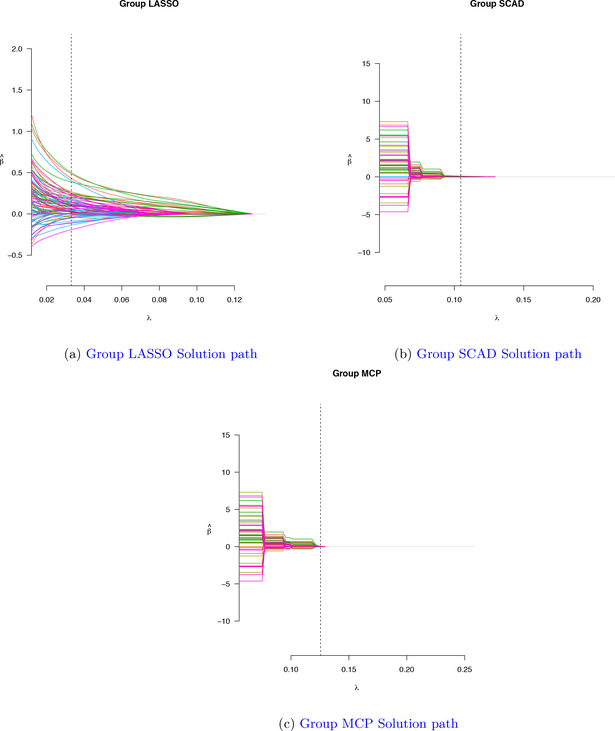
with U ↝ Uniform[0, 1] and G ↝ Gamma(α, α).. Taking into account the censoring status, we simulated censoring times from the exponential distribution: C ↝ Exponential(3). The observed failure time for each observation is the minimum between its survival time T and and its censoring status C. The algorithms described in (3) were implemented to select the appropriate tuning parameter λ to maximize the k-fold CV criterion. Performance of group LASSO with Cox proportional hazard frailty model is compared and contrasted with group SCAD and group MCP. Figure 1 shows an example solution path for group LASSO, group SCAD, and group MCP, respectively. From Table 2, group LASSO selects 8 groups at 0.0294 value of the turning parameter while group SCAD and group MCP highly shrink groups of variables and select only 2 groups at 0.1079 value of the turning paraperter and 1 group at 0.1255 value of the tuning parameter respectively.

Figure 1:

Group Solution path for three methods: Group LASSO, Group SCAD, Group MCP for Simulated data example

Table 2:

Model selection summary for Simulated data example.

Method used	Nonzero coefficients	Nonzero groups	Turning parameter value (λ)
Group LASSO(n=100, p=200)	80	8	0.0294
Group SCAD(n=100, p=200)	20	2	0.1079
Group MCP(n=100, p=200)	10	1	0.1255

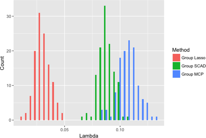
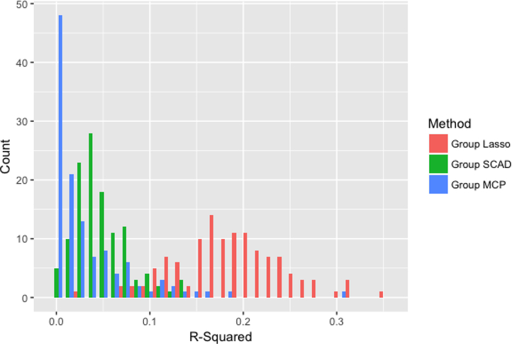
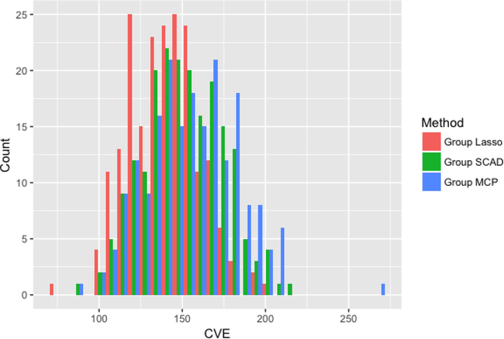
Figures 2–4 compare the performance of the three methods over 100 simulations with summary measures of tuning parameter value choice, cross-validation error, and R², respectively (remembering that this is a simulated data set). Some summary trends appear. Notably for these simulations, group LASSO tends to pick a smaller tuning parameter value, centered around 0.03 compared with 0.09 for group SCAD and 0.10 for group MCP. Considering cross-validation error, the results are similar, with group LASSO demonstrating only slightly better performance (139 for group LASSO compared with 151 for group SCAD and 156 for group MCP) in this set of simulations. R² performance for group LASSO is significantly better, averaging around 0.18 compared with 0.05 for group SCAD and 0.03 for group MCP.

Figure 2:

Distribution of tuning parameter for each of the three methods over 100 simulations.

Figure 4:

Distribution of R-squared values for each of the three methods over 100 simulations.

6.2. Real-world data set example

In this section we have applied the group LASSO method with group frailty for model selection and compare its performance with group SCAD and group MCP to the high dimensional microarray data of diffuse large B-cell lymphoma (DLBCL) patients receiving standard therapy of rituximab plus cyclophosphamide, doxorubicin, vincristine, and prednisolone (R-CHOP) from the US National Cancer Institute of 470+ patients. Gamma frailty has been applied to account for heteregeneity based on risk factors identified in the patient demographic data. Hierarchical clustering has been used to determine gene expression groupings since sparse information is available about these genes and their pathways of relevance to DLBCL. Patients with incomplete demographic or genetic data were excluded, resulting in 470 patient profiles for use in the model. There are 54634 genes described in the dataset; because of computational intensitivity, 5000 genes were selected for the model, and were grouped based on hierarchical clustering into 10 groups, comparable with the simulated dataset. To determine group frailty, eight indices of susceptibility to risk of DLBCL were selected from the demographic data. Based on presence/absence of these characteristics, seven groups were constructed and assigned frailties in order of lowest to highest unmeasured risk related to their demographic data.

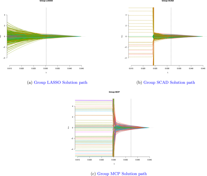
Figure 5 shows an example solution path for group LASSO, group SCAD, and group MCP, respectively. Group LASSO tends to select more groups of variables at a smaller tuning parameter value comparing with group SCAD and group MCP. From Table 3, group LASSO selects 6 groups at 0.0303 value of the turning parameter, group SCAD selects 6 groups at 0.0316 value of the turning paraperter and group MCP selects 3 groups at 0.0372 value of the truning parameter.

Figure 5:

Group Solution path for three methods: Group LASSO, Group SCAD, Group MCP for Real data set data example

Table 3:

Model selection summary for DLBCL dataset example.

Method used	Nonzero coefficients	Nonzero groups	Turning parameter value (λ)
Group LASSO(n=470, p=5000)	636	6	0.0303
Group SCAD(n=470, p=5000)	636	6	0.0316
Group MCP(n=470, p=5000)	278	3	0.0372

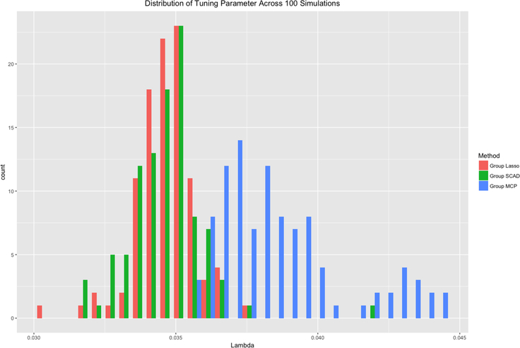
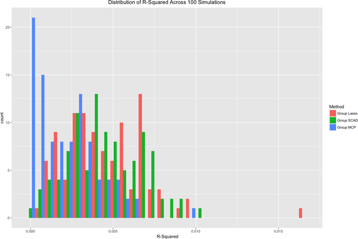
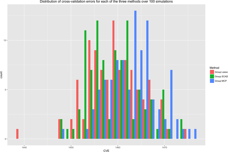
Figures 6–8 compare the performance of the three methods over 100 simulations with summary measures of tuning parameter value choice, cross-validation error, and R-squared, respectively. Some summary trends appear. Notably for these simulations, group LASSO and group SCAD pick a smaller tuning parameter value, centered around 3.5 × 10⁻² compared with 3.9 × 10⁻² for group MCP. R² performance for group LASSO is comparable with group SCAD, with both averaging around 4.5 × 10⁻³ compared with 2.0 × 10⁻³ for group MCP. Considering cross-validation error, the results for group LASSO and group SCAD are also similar, with values around 1459, with group MCP being slightly worse at 1463 in this real dataset. In this case, group LASSO and group SCAD performance are comparable to each other.

Figure 6:

Distribution of tuning parameter for each of the three methods over 100 simulations.

Figure 8:

Distribution of R-squared values for each of the three methods over 100 simulations.

7. Discussion

The relatively poor performance of all group variable selection methods including group LASSO with the real-world dataset highlights problems in this field with tackling these challenges. A lack of informative data about group structure of the genes and their pathways makes describing and implementing their group selections less realistic and weakens the utility of the outcome data. Additionally, the concept of group frailty, be definition constituting unmeasured variation between groups of individuals, is difficult to quantify and requires some degree of knowledge about the differences between groups, even if it is not well measured. Using datasets that were not desigend prospectively to gather the relevant data to highlight frality and grouping structures pose obstacles to rigorous survival analysis and implementation of this modified group LASSO approach.

The limitations of this methodology overlap with the limitations of LASSO. Group LASSO remains a penalization method that is not appropriate for all studies and circumstances and is outperformed at times by ridge regression, least-angle regression (LARS), and the non-negative garrrotte (Yuan and Lin 2007). Even though group LASSO and group frailty make adjustments to account for clustering effects, this method requires a resolution of data and background knowledge that is not available for many data sets and research questions. Future research will continue to elucidate many of these scenarios and make the datasets more amenable to use with group LASSO. While the group LASSO gives a sparse set of groups, if it includes a group of covariates in the model then all coefficients in the group will be nonzero. Sometimes, parsimony both between groups and within each group would be preferred. As an example, if the predictors are genes, it would be useful to identify particularly “important” genes in the pathways of interest. Toward this end (Friedman et al. 2010) focused on the “sparse-group LASSO” wherein they introduced a regularized model for linear regression with L₁ and L₂ penalties. They discussed the sparsity and other regularization properties of the optimal fit for this model and show that it has the desired effect of group-wise and within group sparsity. Even though the group LASSO is an attractive method for variable selection, since it respects the grouping structure in the data, it is generally not selection consistent and also can select groups that are not important in the model (Wei and Huang 2011). To improve the selection results, researchers proposed an adaptive group LASSO method which is a generalization of the adaptive LASSO and requires an initial estimator. They showed that the adaptive group LASSO is consistent in group selection under certain conditions if the group LASSO is used as the initial estimator. In this context, interested researchers may look into the “sparse-group LASSO” or “adaptive group LASSO” for use with the Cox proportional hazard model with frailty when optimizing grouped variable selection as a useful extension from the method proposed and implemented here.

Figure 3:

Distribution of cross-validation errors for each of the three methods over 100 simulations.

Figure 7:

Distribution of cross-validation errors for each of the three methods over 100 simulations.

References

- Akaike H(1973). Information theory and an extension of the maximum likelihood principle. In Petrov BN & Caski F (Eds.), Proceedings of the Second International Symposium on Information Theory. Budapest: Akademiai Kiado, 267–281 [Google Scholar]
- Andersen PK, & Gill RD(1982). Cox’s regression model for counting processes: a large sample study. The Annals of Statistics, 10, 1100–1120 [Google Scholar]
- Antoniadis A & Fan J(2001). Regularization of wavelet approximations (with discussion). J. Am. Statist. Ass, 96, 939–967 [Google Scholar]
- Bakin S(1999). Adaptive regression and model selection in data mining problems. PhD Thesis. Australian National University, Canberra [Google Scholar]
- Breiman L(1995). Better subset regression using the nonnegative garrote. Technometrics, 37, 373–385 [Google Scholar]
- Cai TT(2001). Regularization of wavelet approximations: Discussion. J. Am. Statist. Ass, 96(455), 960–962 [Google Scholar]
- Cox DR(1972). Regression Models and Life-Tables. J. Roy. Statist. Soc. Ser. B, 34, 187–220 [Google Scholar]
- Cox DR & Oakes D.(1984). Analysis of Survival Data. London: Chapman and Hall [Google Scholar]
- Craven P, & Wahba G(1978). Smoothing noisy data with spline functions. Numerische mathematik, 31(4), 377–403 [Google Scholar]
- Fan J & Li R(2002). Selection for Cox’s Proportional Hazards model and Frailty Model. Ann. Statist, 30, 74–99 [Google Scholar]
- Fan J & Li R(2001). Variable selection via nonconcave penalized likelihood and its oracle properties. J. Am. Statist. Ass, 96(456), 1348–1360 [Google Scholar]
- Friedberg JW (2011). Relapsed/refractory diffuse large B-cell lymphoma. ASH Education Program Book, 2011(1), 498–505. [DOI] [PubMed] [Google Scholar]
- Friedman J, Hastie T, & Tibshirani R(2010). A note on the group lasso and a sparse group lasso.
- Fu Z, Ma S, Lin H, Parikh CR, & Zhou B (2017). Penalized variable selection for multi-center competing risks data. Statistics in Biosciences, 9(2), 379–405. [Google Scholar]
- Genkin A, Lewis DD, & Madigan D(2007). Large-scale Bayesian logistic regression for text categorization. Technometrics, 49(3), 291–304 [Google Scholar]
- Gilhodes J, Zemmour C, Ajana S, et al. (2017). Comparison of variable selection methods for high-dimensional survival data with competing events. Computers in biology and medicine, 91, 159–167. [DOI] [PubMed] [Google Scholar]
- Greenland S(2008). Invited commentary: variable selection versus shrinkage in the control of multiple confounders. Am J Epidemiol. 167(5), 523–529 [DOI] [PubMed] [Google Scholar]
- Hoerl AE and Kennard RW.(1970). Ridge regression: biased estimation for nonorthogonal problems. Technometrics, 12(1), 55–67 [Google Scholar]
- Hou J, Paravati A, Hou J, et al. (2018). High-dimensional variable selection and prediction under competing risks with application to SEER-Medicare linked data. Statistics in Medicine, 37(24), 3486–3502 [DOI] [PubMed] [Google Scholar]
- Hougaard P(1986). A class of multivanate failure time distributions. Biometrika, 73(3), 671–678 [Google Scholar]
- Kim J, Sohn I, Jung SH, et al. (2012). Analysis of survival data with group lasso. Communications in Statistics-Simulation and Computation, 41(9), 1593–1605. [Google Scholar]
- Le Cessie S, & Van Houwelingen JC(1992). Ridge estimators in logistic regression. Applied Statistics, 41(1), 191–201 [Google Scholar]
- Leng C, Lin Y, & Wahba G(2006). A note on the lasso and related procedures in model selection. Statistica Sinica, 16, 1273–1284 [Google Scholar]
- Lenz G, Wright G, Dave SS, Xiao W, Powell J, Zhao H, …& Vose J (2008). Stromal gene signatures in large-B-cell lymphomas. New England Journal of Medicine, 359(22), 2313–2323. [DOI] [PMC free article] [PubMed] [Google Scholar]
- Lokhorst J(1999). The lasso and generalised linear models. Honors Project, The University of Adelaide, Australia [Google Scholar]
- Ma L, Teruya-Feldstein J, & Weinberg RA(2007). Tumour invasion and metastasis initiated by microRNA-10b in breast cancer. Nature, 449(7163), 682–688 [DOI] [PubMed] [Google Scholar]
- Martinussen T & Scheike TH(2006). Dynamic Regression Models for Survival Data. Statistics for Biology and Health. New York. Springer [Google Scholar]
- Meier L, Van De Geer S, & Bühlmann P(2008). The group lasso for logistic regression. Journal of the Royal Statistical Society: Series B (Statistical Methodology), 70(1), 53–71 [Google Scholar]
- National Research Council of the National Academies.(2009). Science and Decisions: Advancing Risk Assessment. National Academies Press; [PubMed] [Google Scholar]
- Nielsen GG, Gimll RD, Andersen PK, & Sorensen TI(1992). A counting process approach to maximum likelihood estimation in frailty models. Scandinavian journal of Statistics, 19, 25–43 [Google Scholar]
- Rosenwald A, Wright G, Chan WC, Connors JM, Campo E, Fisher RI, … & Hurt EM (2002). The use of molecular profiling to predict survival after chemotherapy for diffuse large-B-cell lymphoma. New England Journal of Medicine, 346(25), 1937–1947. [DOI] [PubMed] [Google Scholar]
- Roth V(2004). The generalized LASSO. IEEE Transactions on Neural Networks, 15(1), 16–28 [DOI] [PubMed] [Google Scholar]
- Saadati M, Beyersmann J, Kopp-Schneider A, et al. (2018). Prediction accuracy and variable selection for penalized cause-specific hazards models. Biometrical Journal, 60(2), 288–306. [DOI] [PubMed] [Google Scholar]
- Schwarz G(1978). Estimating the dimension of a model. The Annals of Statistics, 6(2), 461–464 [Google Scholar]
- Tibshirani RJ(1996). Regression shrinkage and selection via the lasso. Journal of the Royal Statistical Society: Series B(Methodological), 58, 267–288 [Google Scholar]
- Tibshirani RJ(1997). The lasso method for variable selection in the Cox model. Statistics in Medicine, 16, 385–395 [DOI] [PubMed] [Google Scholar]
- Tibshirani R, & Friedman J(2009). The Elements of Statistical Learning: Data Mining, Inference, and Prediction. 2nd Edition. Springer-Verlag. [Google Scholar]
- Tweedie MCK(1984). An index which distinguishes between some important exponential families. In Statistics: Applications and new directions: Proc. Indian statistical institute golden Jubilee International conference (579), 579–604 [Google Scholar]
- Van der Vaat AW(1998). Asymptotic Statistics. Cambridge University Press [Google Scholar]
- Vaupel JW, Manton KG, & Stallard E(1979). The impact of heterogeneity in individual frailty on the dynamics of mortality. Demography, 16(3), 439–454 [PubMed] [Google Scholar]
- Verweij PJ, & Van Houwelingen HC(1994). Penalized likelihood in Cox regression. Statistics in Medicine, 13(23–24), 2427–2436 [DOI] [PubMed] [Google Scholar]
- Wang H, & Leng C(2008). A note on adaptive group lasso. Computational statistics & data analysis, 52(12), 5277–5286 [Google Scholar]
- Wei F, Huang J, & Li H(2011). Variable selection and estimation in high-dimensional varying-coefficient models. Statistica Sinica, 21(4), 1515–1540. [DOI] [PMC free article] [PubMed] [Google Scholar]
- Yuan M & Lin Y(2006). Model selection and estimation in regression with grouped variables. Journal of the Royal Statistical Society: Series B (Statistical Methodology), 68(1), 49–67 [Google Scholar]
- Yuan M, & Lin Y(2007). On the non-negative garrotte estimator. Journal of the Royal Statistical Society: Series B (Statistical Methodology), 69(2), 143–161 [Google Scholar]
- Yun S, Tseng P, & Toh KC(2011). A block coordinate gradient descent method for regularized convex separable optimization and covariance selection. Mathematical programming, 129(2), 331–355 [Google Scholar]
- Zou H(2006). The adaptive lasso and its oracle properties. Journal of the American Statistical Association, 101(476), 1418–1429 [Google Scholar]
- Zou H, & Hastie T(2005). Regularization and variable selection via the elastic net. Journal of the Royal Statistical Society: Series B (Statistical Methodology), 67(2), 301–320 [Google Scholar]