Negative Binomial mixed models estimated with the maximum likelihood method can be used for longitudinal RNAseq data

Abstract

Time-course RNAseq experiments, where tissues are repeatedly collected from the same subjects, e.g. humans or animals over time or under several different experimental conditions, are becoming more popular due to the reducing sequencing costs. Such designs offer the great potential to identify genes that change over time or progress differently in time across experimental groups. Modelling of the longitudinal gene expression in such time-course RNAseq data is complicated by the serial correlations, missing values due to subject dropout or sequencing errors, long follow up with potentially non-linear progression in time and low number of subjects. Negative Binomial mixed models can address all these issues. However, such models under the maximum likelihood (ML) approach are less popular for RNAseq data due to convergence issues (see, e.g. [1]). We argue in this paper that it is the use of an inaccurate numerical integration method in combination with the typically small sample sizes which causes such mixed models to fail for a great portion of tested genes. We show that when we use the accurate adaptive Gaussian quadrature approach to approximate the integrals over the random-effects terms, we can successfully estimate the model parameters with the maximum likelihood method. Moreover, we show that the boostrap method can be used to preserve the type I error rate in small sample settings. We evaluate empirically the small sample properties of the test statistics and compare with state-of-the-art approaches. The method is applied on a longitudinal mice experiment to study the dynamics in Duchenne Muscular Dystrophy. Contact:s.tsonaka@lumc.nl

Roula Tsonaka is an assistant professor at the Medical Statistics, Department of Biomedical Data Sciences, Leiden University Medical Center. Her research focuses on statistical methods for longitudinal omics data. Pietro Spitali is an assistant professor at the Department of Human Genetics, Leiden University Medical Center. His research focuses on the identification of biomarkers for neuromuscular disorders.

Introduction

Understanding the dynamics of biological processes requires collecting measurements repeatedly in time from the same biological replicate, e.g. patient, animal. For instance, by collecting blood samples at multiple points in time on the same patients which are subsequently sequenced, it gives rise to a set of time series, also known as longitudinal RNAseq data per patient. Modelling the longitudinal gene expression data will lead to the detection of genes which dynamically change over time or genes that show differences in their expression over the whole time period the data are collected (i.e. global difference) between several groups of interest. Such markers can be then potentially further studied as candidates to track disease progression or predict disease milestones. This is also the case in our motivating study, a longitudinal experiment on mice (GEO accession number GSE132741) carried out at the Leiden University Medical Center, in the Netherlands, in order to identify potential biomarkers in blood to track disease progression for Duchenne Mascular Dystrophy (DMD). DMD is an X-linked recessive genetic disease caused by protein truncating mutations in the DMD gene that encodes dystrophin. In this experiment, blood samples were collected longitudinally from 5 healthy and 5 dystrophic mice at 6, 12, 18, 24 and 30 weeks of age, and gene expression was quantified using RNA-seq. Genes for which dystrophic mice evolve differently than the healthy ones can reveal promising therapeutic targets and biomarkers.

To analyse properly such repeatedly measured RNAseq data, we need to address several challenges. First, the serial correlation cannot be ignored. In particular, the gene expression at a certain time point is expected to depend on previous time points . Failure to correct for this will cause biasedly estimated standard errors. This in turn will result in false positive between-group changes and false negative within-subject time changes. Second, in longitudinal studies, measurements are often not collected at the same time points for all subjects and planned measurements may be lost due to sequencing errors or subject dropout. Thereby, unbalanced longitudinal designs arise. In such cases, naive approaches which perform differential expression analysis at each time point separately or ignore the correlation while using all collected data will lead to biassed between- and within-subject changes. The third important complication in the analysis of RNAseq data in general is the typically small number of subjects used due to sequencing costs. This plies unstable estimation of the modelling parameters and test statistics with inflated type I error rates, as the theoretical asymptotic null distributions may not always be correct (see e.g. pg. 98 in [2, p. 98]).

Several methods and software have been developed for RNAseq data, but in their vast majority they handle cross-sectional designs, namely studies where sequencing is done once on samples from independent subjects. For example, the Bioconductor packages edgeR [3], DESeq2 [4] consider Negative Binomial Generalized Linear Models and use empirical Bayes approaches that borrow information across all genes to stabilize the estimation of the gene-wise dispersions due to the small sample size of RNAseq experiments. Alternatively, the logarithm of RNAseq counts per gene can be analysed in terms of linear regression models via the limma-voom pipeline [5]. The mean variance relationship is estimated across all genes and incorprorated into the parameter estimation per gene via weights for each measurement. Similar to edgeR and DESeq2, empirical Bayes is employed to stabilize the estimation of the gene-wise variances. For a more recent review of the available pipelines for the analysis of RNAseq data, see [6]. In the context of longitudinal designs, these pipelines are often erroneously used to test for differences between groups at each time point separately or to make pairwise comparions per group between two time points. In both cases, inefficient use of the data is made which leads to an unnecessary increased multiple testing burden. In addition, all pairwise tests are not interpretable and cannot be used to test for differences in progression between groups (i.e. differences in slopes between groups). A formal definition of the different hypotheses that can be tested in the context of a longitudinal experiment is given in Section 2.2. Finally, bias arises when measurements are missing for some individuals at any time point. Thus, it is obvious that for longitudinal RNAseq experiments methods which use all data at the same time and address the serial correlation should be used.

An important clarification we wish to make is that the designs we study in this paper are different from time-course experiments which collect RNAseq data at multiple time points but on different subjects at each occassion. In fact, in longitudinal designs, there is inherent serial correlation as the same subjects are repeatedly measured in time. Even though time-course experiments with different subjects at each time point can identify genes differentially expressed across different conditions in time, they cannnot be used to study changes due to ageing and disease progression. Examples of pipelines for such time-course experiments are the masigPro [7] which only models the change of mean counts in time but they ignore the serial correlation. Similarly, in timeSeq [8], even though they consider a mixed effects model at the gene level, they model only the between exons correlation and not the serial dependencies. We wish to stress that methods for time-course experiments on independent subjects in time are not appropriate for longitudinal designs.

For the analysis of longitudinal RNAseq data, few methods have been proposed. First, we have the ShrinkBayes [9] which considers (zero-inflated) Negative Binomial Generalized Linear Model (GLM) under the Bayesian approach for the estimation. For the analysis of longitudinal RNAseq data, it offers the possibility to use a single random effect to capture the serial correlations. Under the maximum likelihood (ML) approach, Cui et al. [1] investigated Poisson and Negative Binomial mixed effects models. Generalized linear mixed effects models (GLMMs) offer a flexible modelling framework to properly capture the serial correlation, overdispersion and mean progression per gene. Even though GLMMs are being broadly used in several longitudinal clinical and epidemilogical studies, they are less popular for longitudinal RNAseq data when the ML approach is used for their estimation. Cui et al. [1] have noted that the use of overdispersed Poisson or negative binomial mixed models may not be supported by RNAseq data due to optimization issues they have encountered in their analyses. A popular solution in the setting of correlated RNAseq data is the duplicateCorrelation(.) function of the limma-voom pipeline [10]. The serial correlation of the logarithm of RNAseq counts is estimated using information across all genes and kept fixed at a single value for all genes when testing for differential expression in time or between experimental conditions. Therefore, this approach makes the unrealistic assumption that for all genes the correlation between all pairs of time points is the same. Another approach used in practice is to use the subject identification number as a confounder in the linear predictor in the available pipelines for cross-sectional designs mentioned above [11]. This aims to acknowlegde that a set of measurements originates from the same subject. However, such an approach does not address the serial correlation and it will fail with increasing sample size. Finally, triclustering algorithms have been proposed to detect patterns in three-way gene expression time series data [12].

We argue in this paper that the negative advice of Cui et al. [1] in using Negative Binomial mixed models for RNAseq experiments is two-fold. First, an important complication in the estimation of GLMMs is the evaluation of the marginal likelihood, which requires integration over the unobserved random effects. Such integrals do not have closed-form solution and need to be approximated. Several methods have been proposed to this end, such as Monte Carlo integration [13], Gaussian quadrature approaches [14], Laplace method [15], etc. Standard software for GLMMs typically employs the Laplace method, which is computationally fast, even for several random effects. This is also the case for Negative Binomial mixed models implemented with the function nb.glmm(.) from the R package lme4 [16]. However, such an approach is known to be less accurate and that it can bias the estimation of the model parameters [17, sec. 14.4]. It can also severely affect the evaluation and optimization of the log-likelihood. Therefore, in this paper and motivated by the work of Cui et al. [1], we consider Negative Binomial mixed models where the adaptive Gaussian quadrature method is used to evaluate the integrals over the random effects and can be successfully applied in small sample RNAseq experiments. This is implemented in the function mixedmodel(.) from the R package GLMMadaptive [18].

A second novel contribution of our work in the analysis of longitudinal RNAseq using Negative Binomial mixed models is our solution for small sample inference. Standard pipelines for cross-sectional RNAseq data, have recognised that, with small sample sizes, test statistics have inflated type I error rates [3]. Therefore, they have employed empirical Bayes procedures which borrow information across genes and stabilize thereby the estimation of the gene-wise dispersion parameters. The same problem has been observed for mixed effects models. It is known that with small sample sizes the sampling distribution of the test statistics often deviates from the theoretical distribution leading to inflated type I error rates. In this work, we show that the bootstrap method can be successfully applied to derive inference in small sample settings. An important advantage of our approach is that, depending on the study design, any mixed model can be considered: we may use multiple random effects which may be nested or crossed for clustered designs, and we can model potentially non-linear evolutions in time semi-parametrically using, e.g. natural cubic splines [19]. Besides, mixed models are flexible in modelling the progression in experiments with long follow up or when measurements are collected at irregular points in time for each study participants because the time variable can be treated as numeric and not as a factor. Thereby, polynomials or spline functions of time can be used as covariates. Finally, we can correct for unwanted systematic artifacts such as lane or batch effects or experimental artifacts by correcting for multiple factors.

The paper is organized as follows. In Section 2, we present the Negative Binomial mixed model and we discuss the challenges in its estimation. In Section 3, we discuss issues in the parameter estimation with small sample size. In Section 4, we investigate empirically the performance of the Negative Binomial mixed model for the analysis of small sample longitudinal RNAseq designs. Comparisons with state-of-the-art methods are also made. Finally, in Section 5, we present the analysis of the motivating experiment on a mouse model for Duchene muschular dystrophy designed to study the disease progression.

The Negative Binomial mixed model

The Negative Binomial (NB) distribution has gained popularity in modelling RNAseq gene expression data because it can capture overdispersion and in RNAseq experiments the variance of the counts typically increases with the mean (DESeq [20] and edgeR [3]).

Model formulation

Let (, the longitudinal raw count measurements of gene for the th individual, at the th occassion, and a known -dimensional vector with the covariate information corresponding to the th row of the model matrix , known as design matrix which contains the values of multiple patient characteristics. In particular, in both time-varying (e.g. measurent time, experimental conditions) and time-independent covariates (e.g. treatment group, baseline age, gender, etc.) are allowed. In the longitudinal setting, we use the dimensional vector of random effects , to model the serial correlation with corresponding design matrix . For a specific gene , we assume with probability mass function:

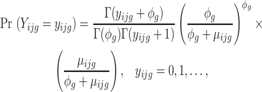where represents the gene-wise dispersion parameter which measures overdispersion and is the gamma function. Based on this parameterization, which is modelled as function of explanatory variables and random effects . In particular using the logarithmic link function:

(1)

where is an offset term with the logarithm of the effective library size derived from edgeR. Throughout the paper, we use the trimmed mean method (TMM) of Robinson et al. [21] to calculate the scaling factors to correct for sequencing depth and potentially composition bias. We assume are the random effects used to model serial correlation with the variance covariance matrix of the random effects. To model flexibly serial correlation splines can also be considered in . Under parameterization (??), it follows . Thus, when , follows the Poisson distribution, i.e. .

Hypothesis testing

An important strength of longitudinal designs is that they can separate the longitudinal from cross-sectional changes (i.e. group changes at a certain time point). Let us assume that in the DMD experiment, briefly introduced in Section 1, the mean counts are modelled as a linear function of the age of the mice, the group and their interaction:

(2)

where is the offset term defined in Section 2.1 above, are the log expected counts for the WT group at baseline, is the change in log expected count for every week that passes by in the WT group and is the change in log expected count between WT and mdx groups for every week that passes by. We will also assume that correlation is captured by a random-intercepts term and is the random-effects variance. Thus, based on model (2), we can test the following hypotheses of interest:

1. Differences in slopes:

   

   which implies that if is rejected, then we have found genes that evolve differently in time, i.e. they have different slopes in time between the two groups.
2. Differences in profiles:

   

   which implies that if is rejected, then we have found genes with different mean profiles in time, i.e. genes that start at different levels and/or evolve differently in time.
3. Differences in levels:

   

   which implies that if is rejected, then we have found genes which start at different levels at baseline irrespective of their progression afterwards.

Note that model (2) can be extended to allow for non-linear progression using splines, e.g. natural cubic splines for the age variable [2, 19, 22].

Estimation

The model parameters for each gene can be estimated via the maximum likelihood approach which requires maximizing the likelihood function:

(3)

In GLMMs, it is known that the integral in (3) with respect to does not have closed-form solution and thus it needs to be approximated. Several methods have been proposed in the literature which are grouped in two categories: (1) methods that approximate the integral numerically and (2) methods that approximate the integrand such that the integral of the approximation is then solved. In the first category, we have the adaptive and non-adaptive Gaussian quadrature approach [14] and Monte Carlo integration [13]. In the second category, we have the Laplace’s method [15] and quasi-likelihood approaches: penalized quasi-likelihood [23–25] and marginal quasi-likelihood [26] and their extensions (MQL2, PQL2 and corrected PQL). Methods in the second category are known to behave poorly in various settings, e.g. with few repeated measurements, high between samples heterogeneity leading to parameter estimates with an appreciable downward asymptotic bias. On the contrary, methods in the first category are known to be more accurate though more computationally intensive. For the rest, we will concentrate our discussion on methods that are available in R for the Negative Binomial distribution. In particular, the Laplace method is used in function glmm.nb(.) in lme4 [16] or glmmTMB [27] to fit Negative Binomial mixed models. The Laplace approximation is based on a quadratic approximation of the log-integrand. It is known to be fast, however it may lose in accuracy, especially when limited information is available and short follow-up (e.g., [17], sec. 14.4). Based on our experience, Negative Binomial mixed models with the Laplace method often fail for longitudinal RNAseq data. Cui et al. [1] have reported similar behaviour.

Alternatively, the Adaptive- Gaussian–Hermite (AGH) quadrature method which is known to be more accurate can be used. Let the integrand as a function of which needs to be approximated in (3). Note that here for notational simplicity we assume a single random effects term per gene. Gaussian quadrature methods are used to approximate integrals of the form , by a weighted sum, i.e.

(4)

where is a known function, is the standard normal density, is the order of the approximation, i.e. the higher the more accurate the approximation will be. Then are the quadrature points, derived as solutions to the th-order Hermite polynomial, and are appropriately chosen weights. Both the quadrature points and weights are considered fixed and known. If is concentrated far from 0, or if the spread in is different than that for the weight function , then we can get a very poor approximation. In this case, we need to appropriately rescale the subject-specific integrands in the log-likelihood (3) such that the quadrature points are located where most of the mass of is located. This can be achieved by using as quadrature points:

and weights:

in (4). Note that and are not any more fixed and known. They need to be estimated iteratively, making thereby the optimization of (3) rather computationally intensive. Therefore, the numerical integration in (4) using and is more than with the fixed and .

In the special case where 1 quadrature point is used, AGH corresponds to the Laplace approximation. In fact the integral (4) is evaluated using

Therefore, the approximation using the Laplace method is inferior to AGH.

Small sample inference

Even though sequencing costs are dropping, the number of subjects sequenced longitudinally still remains low. This implies that there is limited information and the assumed sampling distribution of the test statistics may not be correct. In cross-sectional RNAseq studies, it has been observed that gene-wise dispersion related parameters are not reliably estimated in this case. Thus, the common practice to overcome the small sample issue is to utilize prior information across genes to estimate the gene-wise dispersions using an empirical Bayes estimation step. Thereby, we can derive test statistics with type I error close to the nominal level. This method is used in pipelines developed for cross-sectional (such as edgeR and DEseq2). In longitudinal studies, where random effects models are used to capture the serial correlation, bias is observed not only in the estimation of the dispersion parameter but also the random-effects variance. We will discuss this in Section 4 in the context of our simulation studies.

In this work, we explore an alternative procedure to derive the proper sampling distribution of test statistics, namely via parametric Bootstrap [28]. Our motivation in this direction are certain limitations of the current practice to address the small sample issue in RNAseq experiments, i.e. the empirical Bayes step. First, such a practice requires that all genes are analysed jointly, which can be rather computationally demanding, e.g. in the Bayesian setting for ShrinkBayes. Second, depending on the complexity of the study design (e.g. non-linear profiles in time and family studies) multiple random effects may be needed and this implies that custom-made software is needed each time to stabilize the estimation of the dispersion and variance related parameters.

In particular, let us assume that model (2) is used to describe the progression of each gene in the DMD experiment and that we are interested to identify genes with different mean profiles in time between WT and mdx groups, i.e. we want to test the hypothesis:

This hypothesis can be tested using the likelihood ratio test (LRT) statistic or multivariate Wald test statistic (see e.g. [29], Chapter 6). The LRT is given by

where is the log-likelihood value under the null hypothesis and is the value under the alternative hypothesis. It follows from classical likelihood theory (see e.g. [30], Chapter 9) that under the null hypothesis the follows asymptotically a chi-squared distribution with degrees of freedom equal to the difference in the number of parameters between the models under the null and alternative hypothesis. The Wald statistic is given by

where is the contrast matrix and is the variance-covariance matrix of the maximum likelihood estimates .

Figure 3 .

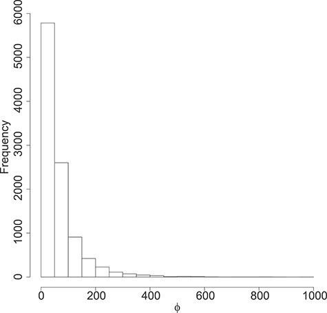
DMD mice experiment analysis: Histogram of the estimated dispersion parameters per gene.

The procedure is as follows:

1. Model (2) is fitted on the data and the estimates are derived.

2. Let the parameter vector under the null hypothesis derived from by setting . Simulate datasets under the null, i.e. Negative Binomial mixed model .

3. Compute the test statistic on each dataset: .

4. Compute -value:

   

Simulation Study

We have set up a simulation study with the following objectives: (1) Evaluate the type I error rate of the test statistics (i.e., Wald test and Likelihood ratio test) with increasing sample size and correlation structure for the standard Negative Binomial mixed model when the theoreticall null distribution is used for the computation of the -values or bootstrap, (2) compare the false positive rate of the Negative Binomial mixed model when multiple genes are studied, as in any real RNAseq experiment, with the state-of-the-art Maximum Likelihood approaches edgeR and duplicateCorrelation(.) function in the limma-voom pipeline. In particular, motivated by the DMD experiment which will be presented in detail in Section 5 we estimate the proportion false discoveries when 50% of the simulated genes are assumed to exhibit differential expression between the two groups.

Type I error rate control

We have simulated longitudinal count measurements from the Negative Binomial mixed model, described in Section 2, with mean model given by

(5)

where denotes the timing of the th repeated measurement of subject and is the group indicator for the th subject. Motivated from the DMD experiment we have chosen and . We have set up 12 scenarios to evaluate empirically the type I error rate for the Wald test and Likelihood ratio test where we considered different choices for the number of subjects, i.e. and the size of between-subject variability, i.e.

For each scenario, 5000 datasets are simulated, and type I error is computed as the number of times the null hypothesis is rejected. This hypothesis is tested using the standard likelihood ratio test and the Wald test on 2 degrees of freedom and their corresponding bootstrap versions with .

Type I error rate control: Results

In Figure 1 and Table 1, we present type I error rates under the settings described in Section 4.1 over 5000 datasets. In Table 2, we present results on the quality of the estimated parameters. We observe that the standard LRT and Wald tests are anti-conservative for small sample sizes while the type I error gets closer to nominal levels when . Similarly, the type I error gets inflated with the strength of the within-subject correlation. On the contrary when the null distribution is estimated empirically via the bootstrap method the type I error is at the nominal level across the different scenarios.

Figure 1 .

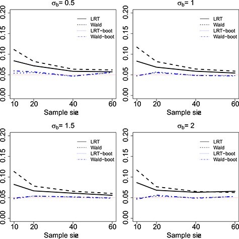
Type I error rate of LRT and Wald statistics when using the asymptotic (black lines) and their corresponding bootsrap-based null distribution (blue lines) for testing versus or . Each panel corresponds to a different size of the serial correlation captured by the random effects standard deviation .

Table 1.

Type I error rate of LRT and Wald statistics when using the asymptotic and their corresponding bootstrap-based null distribution for testing versus or . We have varied the serial correlation captured by the random effects standard deviation and the sample size

	Test	= 10	= 20	= 40	= 60
	LRT	0.084	0.072	0.058	0.057
	Wald	0.111	0.082	0.064	0.062
	LRT-boot	0.054	0.055	0.047	0.055
	Wald-boot	0.059	0.057	0.047	0.056
	LRT	0.083	0.068	0.059	0.054
	Wald	0.117	0.082	0.064	0.059
	LRT-boot	0.047	0.057	0.048	0.048
	Wald-boot	0.048	0.055	0.048	0.047
	LRT	0.082	0.066	0.061	0.056
	Wald	0.113	0.078	0.065	0.060
	LRT-boot	0.047	0.054	0.054	0.054
	Wald-boot	0.049	0.054	0.052	0.049
	LRT	0.086	0.068	0.063	0.065
	Wald	0.117	0.076	0.065	0.062
	LRT-boot	0.049	0.054	0.050	0.053
	Wald-boot	0.046	0.056	0.049	0.053

Table 2.

Parameter estimates: mean, standard deviation and root mean squared error in parentheses over 5000 datasets for the Negative Binomial mixed model (5). We have varied the serial correlation captured by the random effects standard deviation and the sample size

Pars	True	= 10	= 20	= 40	= 60
	4.00	3.991(0.287)(0.287)	3.997(0.202)(0.202)	3.998(0.144)(0.144)	4.000(0.117)(0.117)
	1.00	1.001(0.147)(0.147)	0.999(0.106)(0.106)	1.000(0.073)(0.073)	0.998(0.060)(0.060)
	0.00	-0.001(0.413)(0.413)	-0.001(0.290)(0.290)	0.002(0.206)(0.206)	0.000(0.167)(0.167)
	0.00	0.000(0.208)(0.208)	0.001(0.148)(0.148)	-0.001(0.103)(0.103)	0.001(0.086)(0.086)
	0.25	0.193(0.122)(0.135)	0.221(0.091)(0.095)	0.237(0.067)(0.068)	0.241(0.056)(0.056)
	4.00	4.46(1.111)(1.202)	4.209(0.690)(0.721)	4.099(0.466)(0.476)	4.064(0.372)(0.378)
	4.00	3.991(0.485)(0.485)	3.996(0.341)(0.341)	3.997(0.243)(0.243)	3.997(0.197)(0.197)
	1.00	1.001(0.148)(0.148)	1.000(0.106)(0.106)	1.000(0.074)(0.074)	1.001(0.060)(0.060)
	0.00	-0.004(0.692)(0.692)	0.001(0.483)(0.483)	0.004(0.346)(0.346)	0.002(0.283)(0.283)
	0.00	0.003(0.210)(0.210)	-0.001(0.151)(0.151)	0.000(0.105)(0.105)	-0.001(0.086)(0.086)
	1.00	0.802(0.431)(0.474)	0.904(0.319)(0.333)	0.952(0.231)(0.236)	0.969(0.192)(0.194)
	4.00	4.466(1.131)(1.223)	4.212(0.696)(0.728)	4.103(0.475)(0.486)	4.073(0.381)(0.388)
	4.00	3.991(0.697)(0.697)	3.995(0.491)(0.491)	3.999(0.348)(0.348)	4.000(0.283)(0.283)
	1.00	1.001(0.147)(0.147)	0.999(0.107)(0.107)	0.999(0.074)(0.074)	0.999(0.062)(0.062)
	0.00	-0.004(0.992)(0.992)	-0.001(0.695)(0.695)	0.005(0.499)(0.499)	-0.001(0.403)(0.403)
	0.00	0.002(0.211)(0.211)	0.003(0.153)(0.153)	0.002(0.106)(0.106)	0.002(0.088)(0.088)
	2.25	1.817(0.947)(1.041)	2.044(0.703)(0.732)	2.149(0.506)(0.516)	2.184(0.422)(0.427)
	4.00	4.474(1.13)(1.225)	4.224(0.718)(0.752)	4.105(0.486)(0.497)	4.076(0.388)(0.395)
	4.00	3.99(0.922)(0.922)	3.994(0.648)(0.648)	3.994(0.458)(0.458)	3.996(0.372)(0.372)
	1.00	0.999(0.154)(0.154)	1.000(0.109)(0.109)	1.001(0.077)(0.077)	1.001(0.063)(0.063)
	0.00	-0.004(1.308)(1.308)	0.005(0.919)(0.919)	0.014(0.660)(0.660)	0.001(0.531)(0.531)
	0.00	0.002(0.217)(0.217)	0.000(0.153)(0.153)	-0.001(0.108)(0.108)	0.000(0.090)(0.090)
	4.00	3.234(1.679)(1.845)	3.631(1.244)(1.297)	3.814(0.896)(0.915)	3.864(0.737)(0.749)
	4.00	4.505(1.193)(1.295)	4.240(0.741)(0.778)	4.120(0.505)(0.519)	4.081(0.397)(0.405)

As expected in the sample settings we have considered, the random effects variance and dispersion are under- and overestimated, respectively.

False discovery rate control

In Section 4.1 above, we have evaluated the type I error rate of the LRT and Wald tests when 1 gene is tested. Here we will compare our proposal to analyse RNAseq counts using Negative Binomial mixed models and bootstrap per gene with existing pipelines: edgeR and limma-voom.

Specifically, we will consider the setting where 500 genes are simulated for the same subject , . We assume that the subjects are assigned to two groups and are followed up at 5 time points. Repeated count data are simulated for each gene from the model:

(6)

where , for all , for of the genes and for the remaining differentially expressed genes. We have also set for all genes and we have considered four scenarios for the serial correlation, i.e. was set at and 2. For the scaling factors we have assumed . These scaling factors have been kept fixed for all the pipelines to make fair comparions. For subjects we have simulated 50 longitudinal datasets with 500 genes each. Our goal is to evaluate the False Positive Rate for the hypothesis:

across different pipelines. In particular, on each dataset we applied (i) the negative binomial mixed model (6) per gene with 1000 bootstrap samples to estimate the -value per gene for the LRT and Wald test, (ii) edgeR where the hypothesis of interest is tested using the LRT or the quasi -test and (iii) limma-voom where we used the moderated -test. The gene-wise -values per dataset have been corrected for multiple testing using the false discovery rate (FDR) approach [31].

False discovery rate control: results

The mean proportions of false discoveries (out of all discoveries) (FDR) over the 50 datasets in the four scenarios considered per method are given in Table 3, the mean proportions of true discoveries are given in Table 5, the mean proportions of discoveries are given in Table 4 and the mean proportions of true negative discoveries are given in Table 6. A graphical presentation of all the results across the different methods is given in Figure 2.

Table 3.

Mean proportion false discoveries over 50 datasets for LRT and Wald statistics from the Negative Binomial mixed model when using the asymptotic (“LRT” and “W”, respectively) and their corresponding bootstrap-based null distribution (“LRT-boot” and “W-boot”, respectively) for testing versus or . We have made comparisons with the -test statistic in limma-voom approach (“F-voom”) and LRT and -test statistic in edgeR (“LRT-edgeR” and “W-edgeR”, respectively)

	LRT	LRT-edgeR	F-edgeR	W	LRT-boot	W-boot	F-voom
0.5	0.017	0.000	0.000	0.026	0.010	0.010	0.002
1.5	0.016	0.195	0.167	0.026	0.008	0.007	0.422
2.0	0.017	0.192	0.169	0.028	0.007	0.007	0.474

Table 5.

Mean proportion true discoveries for LRT and Wald statistics from the negative binomial mixed model when using the asymptotic (“LRT” and “W”, respectively) and their corresponding bootstrap-based null distribution (“LRT-boot” and “W-boot”, respectively) for testing versus or . We have made comparisons with the -test statistic in limma-voom approach (“F-voom”) and LRT and -test statistic in edgeR (“LRT-edgeR” and “W-edgeR’, respectively)

	LRT	LRT-edgeR	F-edgeR	W	LRT-boot	W-boot	F-voom
0.5	0.465	0.000	0.000	0.484	0.431	0.430	0.001
1.5	0.498	0.499	0.497	0.500	0.498	0.498	0.081
2.0	0.475	0.500	0.500	0.500	0.499	0.499	0.081

Table 4.

Mean proportion discoveries for LRT and Wald statistics of the Negative Binomial mixed model when using the asymptotic (“LRT” and “W”, respectively) and their corresponding bootstrap-based null distribution (“LRT-boot” and “W-boot”, respectively) for testing versus or . We have made comparisons with the -test statistic in limma-voom approach (“F-voom”) and LRT and -test statistic in edgeR (‘LRT-edgeR’ and ‘W-edgeR’, respectively)

	LRT	LRT-edgeR	F-edgeR	W	LRT-boot	W-boot	F-voom
0.5	0.482	0.000	0.000	0.511	0.441	0.441	0.003
1.5	0.514	0.694	0.665	0.526	0.506	0.505	0.503
2.0	0.492	0.692	0.668	0.528	0.506	0.506	0.554

Table 6.

Mean proportion true negative discoveries for LRT and Wald statistics from the Negative Binomial mixed model when using the asymptotic (‘LRT’ and ‘W’, respectively) and their corresponding bootsrap-based null distribution (“LRT-boot” and “W-boot”, respectively) for testing versus or . We have made comparisons with the -test statistic in limma-voom approach (“F-voom”) and LRT and -test statistic in edgeR (“LRT-edgeR” and “W-edgeR”, respectively)

	LRT	LRT-edgeR	F-edgeR	W	LRT-boot	W-boot	F-voom
0.5	0.483	0.500	0.500	0.474	0.490	0.490	0.498
1.5	0.484	0.305	0.333	0.474	0.492	0.493	0.078
2.0	0.483	0.308	0.332	0.472	0.493	0.494	0.026

Figure 2 .

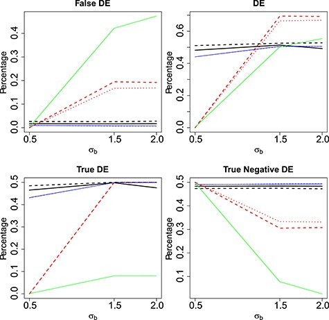
Mean proportion false discoveries of LRT and Wald statistics when using the asymptotic (black) and their corresponding bootstrap-based null distribution (blue) for testing versus or . We have also compared with the F-test statistic in limma-voom approach (green) and LRT and -test statistic in edgeR (red). Each panel corresponds to proportion false discoveries (top left), proportion discoveries (top right), proportion true discoveries (bottom left) and proportion true negative discoveries (bottom right).

We observe that as the serial correlation increases, the FDR for edgeR which does not model the correlation in the data increases. Similarly, for the limma-voom, even though the correlation is modelled via random effects, the FDR increases with the size of the correlation, suggesting that misspecification of the correlation in the data can severely impact the analysis. The lowest FDR across all scenarios is achieved when the boostrap method is used. Our simulation in combination with the type I error results per gene suggest that the Negative Binomial mixed model can be used for the analysis of each gene separately as long as the bootstrap method is used.

The R code used to simulate the data used in this section along with an illustration to apply the Negative Binomial mixed model with the bootstrap sampling is available at https://github.com/rtsonaka/NBmixed_RNAseq.

Characterising disease progression in Duchenne Muschular Dystrophy: A longitudinal RNAseq experiment on mice

We will analyse RNAseq data from a longitudinal experiment on mice carried out at the Leiden University Medical Center (GEO accession number GSE132741). The aim is to identify biomarkers of disease progression in the mdx mouse model of DMD carrying a nonsense mutaiton in exon 23. DMD is a rare neuromuscular disorder caused by protein truncating mutations in the DMD gene that encodes dystrophin. Its progression is characterised by a process of muscle degeneration and regeneration which results in an increasing replacement of muscle tissue with fibrotic tissue, leading to loss of muscle function and premature death. Progression of DMD is currently monitored through physical tests or muscular biopsies, both of which are rather invasive. In search for less invasive ways to track disease progression, blood samples have been collected longitudinally from 5 dystrophin-lacking (mdx) mice and 5 wild type (WT) mice at 6, 12, 18, 24 and 30 weeks of age. For 2 mice in the mdx group, 4 planned samples have not been collected due to mouse dropout. Gene expression is subsequently quantified via RNA-seq.

After an initial pre-processing and filtering 10348 genes are considered for further analysis. Specifically, low count genes have been filtered out and we kept genes with at least 5 counts per million in at least 10% of the samples. These genes are further normalized using the TMM approach of Robinson and Oshlack (2010) [21].

The Negative Binomial mixed model introduced in Section 2 is applied on each gene where the logarithm of mean counts of mouse () at the th occassion () is modelled as a linear function of age, group and their interaction:

(7)

where , is an offset term with scaling factors to correct for sequencing depth and potentially composition bias. We assume . Finally, captures the extra overdispersion per gene .

Our goal is to identify genes that show a differential mean profiles in time, i.e. we want to test for and each . This corresponds to hypothesis 2 in Section 2.2. This hypothesis has been tested using the Likelihood ratio test and the corresponding -value is estimated using bootstrap as described in Section 3 with .

Results

The distribution of the estimated standard deviation for the random effects is shown is Figure 4.

Figure 4 .

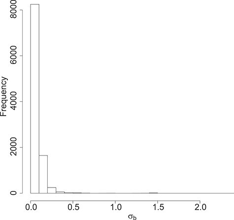
DMD mice experiment analysis: Histogram of the estimated standard deviation for the random effects per gene.

Note that, as expected in mice experiments, the estimated variances are rather small compared to human studies.

Our analysis has identified 246 genes that show differential progression between the two groups after FDR multiple testing correction.

The distribution of the bootstrap-based -values is shown is Figure 5.

Figure 5 .

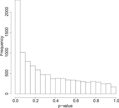
DMD mice experiment analysis: Histogram of the bootstrap-based -values to test the hypothesis for each gene .

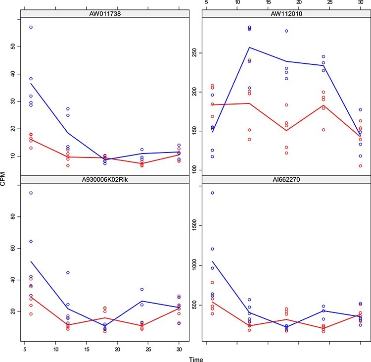
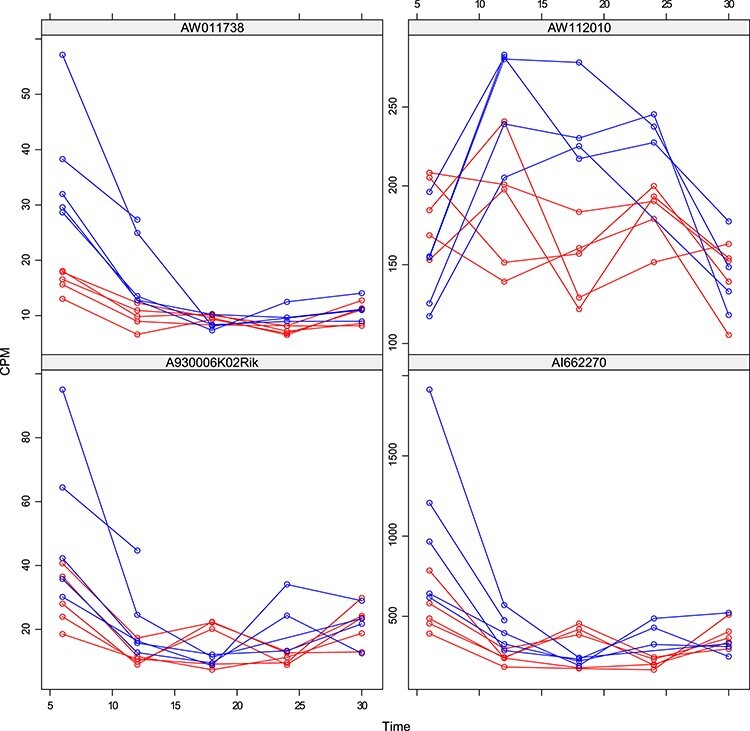
The observed longitudinal trajectories for four randomly selected genes with statistically significant differential mean profiles between WT and mdx are given in Figure 10. The corresponding fitted mean profiles are shown in Figure 9. For these four genes, we tested further the hypotheses about differences in levels and in slopes (i.e. Hypothesis (3) and (1) in Section 2, respectively). The -values for these hypotheses at each time point are given in Tables 7 and 8.

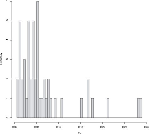
Figure 7 .

DMD mice experiment analysis: Histogram of the estimated random effects standard deviations for the genes detected by the Negative Binomial mixed model and not by the limma-voom.

Figure 6 .

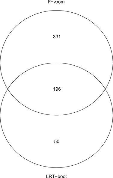
DMD mice experiment analysis: Venn diagram for the differentially expressed genes based on the Negative Binomial mixed model (“LRT-boot”) and limma-voom (‘F-voom’).

Table 7.

-values for the hypothesis of no group changes at each time point

Gene	Week 6	Week 12	Week 18	Week 24	Week 30
A930006K02Rik	0.008	0.003	0.101	0.000	0.905
AI662270	0.000	0.001	0.045	0.000	0.635
AW011738	0.000	0.000	0.541	0.005	0.463
AW112010	0.019	0.000	0.000	0.017	0.889

Table 8.

-values for the hypothesis of no differences in slopes at each time point versus Week 6

Gene	Week 6	Week 12	Week 18	Week 24	Week 30
A930006K02Rik	0.008	0.797	0.001	0.298	0.049
AI662270	0.000	0.529	0.000	0.811	0.001
AW011738	0.000	0.244	0.000	0.014	0.000
AW112010	0.019	0.000	0.000	0.000	0.060

According to the results of the simulation study described in Section 4, the duplicateCorrelation(.) function in limma-voom can be liberal and lose power in certain scenarios. However, for the purposes of illustration, we have analysed the same dataset using limma-voom and compared the results. The overlap in the number of genes with statistically different mean profiles is shown in Figure 6. Note that using limma-voom the mean (over all genes) serial correlation is estimated at 0.090 and kept fixed across all genes.

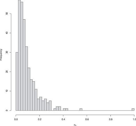
Figure 8 .

DMD mice experiment analysis: Histogram of the estimated random effects standard deviations for the genes detected by limma-voom and not by the Negative Binomial mixed model.

To understand better the differences between the two methods, we have studied the size of estimated serial correlation in the genes detected by each one alone and jointly. In particular, in Figure 7, we observe the size of the estimated random effects standard deviations for the genes detected by the Negative Binomial mixed model and not by the limma-voom. In this set of genes, the estimated values for are lower than the low correlation setting we have considered in our simulation study. In accordance with our simulation study results, limma-voom is conservative and has lower power than the Negative Binomial mixed model. Figure 8 presents the distribution of the estimated random effects standard deviations for the genes detected by the limma-voom and not by the Negative Binomial mixed model. In this set of genes, the estimated values for get closer to our moderate correlation setting we have considered in our simulation study. In accordance with our simulation study results, limma-voom is liberal while having lower power than the Negative Binomial mixed model.

Figure 9 .

DMD mice experiment analysis: Fitted mean cpm profiles for four randomly selected genes with differential profiles between WT and mdx mice.

Figure 10 .

DMD mice experiment analysis: Spaghetti plots for four randomly selected genes with differential profiles between WT and mdx mice.

Discussion

We have shown that Negative Binomial mixed models can be successfully used in the analysis of small longitudinal RNAseq datasets. It is the combination of the numerical integration method and the small sample size which have made such models estimated under the Maximum Likelihood approach less popular. We have shown that careful estimation of the sampling distribution of the test statistic using bootstrap leads to stable estimation of the model parameters and preserves the type I error. Therefore, we do not need to exploit an empirical Bayes step where all genes are modelled at the same time to estimate a common mean-variance trend as in edgeR or ShrinkBayes. Often this step is not well understood by the end-user and the implication has not been yet evaluated.

Our simulation in combination with the type I error results per gene suggect that the Negative Binomial mixed model can be used for the analysis of each gene separately as long as the bootstrap method is used.

Key Points

• In longitudinal RNAseq studies the serial correlations should not be ignored, otherwise, inflated type I errors rates are observed.

• Negative Binomial mixed effects models can be used for the analysis of correlated RNAseq data, provided that the accurate adaptive Gaussian quadrature approach is used to approximate the integrals over the random effects.

• In small sample settings, the asymptotic null distribution of the test statistics may not hold and thus the boostrap method is proposed to empirically derive the sampling distribution of the test statistics.

• Negative Binomial mixed effect models in combination with parametric boostrap can be used to model complex designs. For instance, nested random effects or splines can be used to model clustered data or non-linear evolutions, respectively.

Roula Tsonaka is assistant professor at the Medical Statistics section, Department of Biomedical Data Sciences, Leiden University Medical Center. Her research focuses on statistical methods for longitudinal omics data.

Pietro Spitali is assistant professor at the Department of Human Genetics, Leiden University Medical Center. His research focuses on the identification of biomarkers for neuromuscular disorders.

References

- 1. Cui S, Ji T, Li J, et al. What if we ignore the random effects when analyzing RNA-seq data in a multifactor experiment. Stat Appl Genet Mol Biol 2016; 15:87–105. [DOI] [PubMed] [Google Scholar]
- 2. Fitzmaurice GM, Laird NM, Ware JH. Applied Longitudinal Analysis. Hoboken, NJ: Wiley-Interscience, 2004. [Google Scholar]
- 3. Robinson MD, McCarthy DJ, Smyth GK. edgeR: a bioconductor package for differential expression analysis of digital gene expression data. Bioinformatics 2010; 26:139–40. [DOI] [PMC free article] [PubMed] [Google Scholar]
- 4. Love MI, Huber W, Anders S. Moderated estimation of fold change and dispersion for RNA-seq data with DESeq2. Genome Biol 2014; 15:550. [DOI] [PMC free article] [PubMed] [Google Scholar]
- 5. Law CW, Chen Y, Shi W, et al. Voom: precision weights unlock linear model analysis tools for RNA-seq read counts. Genome Biol 2014; 15:R29. [DOI] [PMC free article] [PubMed] [Google Scholar]
- 6. van den Berge K, Hembach KM, Soneson C, et al. RNA sequencing data: Hitchhiker’s guide to expression analysis. Annu Rev Biomed Data Sci 2019; 2:139–73. [Google Scholar]
- 7. Nueda MJ, Tarazona S, Conesa A. Next maSigPro: updating maSigPro bioconductor package for RNA-seq time series. Bioinformatics 2014; 30:2598–602. [DOI] [PMC free article] [PubMed] [Google Scholar]
- 8. Sun X, Dalpiaz D, Wu D, et al. Statistical inference for time course RNA-Seq data using a negative binomial mixed-effect model. BMC Bioinformatics 2016; 17:324. [DOI] [PMC free article] [PubMed] [Google Scholar]
- 9. van de Wiel MA, Neerincx M, Buffart TE, et al. ShrinkBayes: a versatile R-package for analysis of count-based sequencing data in complex study designs. BMC Bioinformatics 2014; 15:116. [DOI] [PMC free article] [PubMed] [Google Scholar]
- 10. Smyth GK, Michaud J, Scott H. The use of within-array replicate spots for assessing differential expression in microarray experiments. Bioinformatics 2005; 21:2067–75. [DOI] [PubMed] [Google Scholar]
- 11. Chen Y, McCarthy D, Ritchie M, et al. edgeR: Differential Analysis of Sequence Read Count Data User’s Guide, 2020. https://bioconductor.org/packages/release/bioc/vignettes/edgeR/inst/doc/edgeRUsersGuide.pdf. (29 September 2020, date last accessed).
- 12. Henriques R, Madeira SC. Triclustering algorithms for three-dimensional data analysis: a comprehensive survey. ACM Comput Surv 2018; 51:1–43. [Google Scholar]
- 13. Booth J, Hobert J. Maximizing generalized linear mixed model likelihoods with an automated Monte Carlo EM algorithm. J R Stat Soc Series B Stat Methodology 1999; 61:265–85. [Google Scholar]
- 14. Pinheiro PC, Bates DM. Approximations to the log-likelihood function in the nonlinear mixed-effects model. J Comput Graph Stat 1995; 4:12–35. [Google Scholar]
- 15. Tierny L, Kadane JB. Accurate approximations for posterior moments and marginal densities. J Am Stat Assoc 1986; 81:82–6. [Google Scholar]
- 16. Bates D, Maechler M, Bolker B, et al. Fitting linear mixed-effects models using lme4. J Stat Softw 2015; 67:1–48. [Google Scholar]
- 17. McCulloch CE, Searle SR, Neuhaus JM. Generalized, Linear, and Mixed Models, 2nd edn. New York: Wiley, 2008. [Google Scholar]
- 18. Rizopoulos D. GLMMadaptive: Generalized Linear Mixed Models Using Adaptive Gaussian Quadrature. R Package Version 0.6-5, 2019. https://CRAN.R-project.org/package=GLMMadaptive. (29 September 2020, date last accessed).
- 19. Hastie TJ. Generalized additive models. In: Chambers, JM, Hastie TJ (eds). Statistical Models in S. California: Wadsworth & Brooks/Cole, 1992. [Google Scholar]
- 20. Anders S, Huber W. Differential expression analysis for sequence count data. Genome Biol 2010; 11:R106. [DOI] [PMC free article] [PubMed] [Google Scholar]
- 21. Robinson MD, Oshlack A. A scaling normalization method for differential expression analysis of RNA-seq data. Genome Biol 2010; 11:R25. [DOI] [PMC free article] [PubMed] [Google Scholar]
- 22. Wood SN. Generalized Additive Models: An Introduction with R, 2nd edn. CRC Press, 2017. [Google Scholar]
- 23. Breslow NE, Clayton DG. Approximate inference in generalized linear mixed models. J Amer Statist Soc 1993; 88:9–25. [Google Scholar]
- 24. Schall R. Estimation in generalised linear models with random effects. Biometrika 1991; 78:719–27. [Google Scholar]
- 25. Stiratelli R, Laird N, Ware JH. Random-effects model for serial observations with binary response. Biometrics 1984; 40:961–71. [PubMed] [Google Scholar]
- 26. Goldstein H. Nonlinear multilevel models, with an application to discrete response data. Biometrika 1991; 78:45–51. [Google Scholar]
- 27. Kristensen K, Nielsen A, Berg CW, et al. TMB: automatic differentiation and Laplace approximation. J Stat Softw 2016; 70:1–21. [Google Scholar]
- 28. Efron B, Tibshirani R. An Introduction to the Bootstrap. London: Chapman and Hall, 1993. [Google Scholar]
- 29. Verbeke G, Molenberghs G. Linear Mixed Models for Longitudinal Data. Springer Series in Statistics. New York: Springer, 2000. [Google Scholar]
- 30. Cox D, Hinkley D. Theoretical Statistics. New York: Chapman and Hall/CRC, 1990. [Google Scholar]
- 31. Benjamini Y, Hochberg Y. Controlling the false discovery rate: a practical and powerful approach to multiple testing. J. Roy. Statist. Soc. Ser. B 1995; 57:289–300. [Google Scholar]