Denoising of Diffusion MRI Data via Graph Framelet Matching in x-q Space

Abstract

Diffusion magnetic resonance imaging (DMRI) suffers from lower signal-to-noise-ratio (SNR) due to MR signal attenuation associated with the motion of water molecules. To improve SNR, the non-local means (NLM) algorithm has demonstrated state-of-the-art performance in noise reduction. However, existing NLM algorithms do not take into account explicitly the fact that DMRI signal can vary significantly with local fiber orientations. Applying NLM naïvely can hence blur subtle structures and aggravate partial volume effects. To overcome this limitation, we improve NLM by performing neighborhood matching in non-flat domains and removing noise with information from both x-space (spatial domain) and q-space (wavevector domain). Specifically, we first encode the q-space sampling domain using a graph. We then perform graph framelet transforms to extract robust rotation-invariant features for each sampling point in x-q space. The resulting features are employed for robust neighborhood matching to locate recurrent information. Finally, we remove noise via an NLM framework. To adapt to the various types of noise in multi-coil MR imaging, we transform the signal before denoising so that it is Gaussian-distributed, allowing noise removal to be carried out in an unbiased manner. Our method is able to more effectively locate recurrent information in white matter structures with different orientations, avoiding the blurring effects caused by naïvely applying NLM. Experiments on synthetic, repetitively-acquired, and infant DMRI data demonstrate that our method is able to preserve subtle structures while effectively removing noise.

I. Introduction

DIFFUSION magnetic resonance imaging (DMRI) plays a vital role in understanding white matter development and pathology in the human brain [1], [2]. For example, various studies have utilized DMRI in investigating the asynchronous and protracted nature of brain development in the first years of life [1]. DMRI tractography was used in [2] to study the small-world nature of the brain structural network in the first two years of life. DMRI was also employed to investigate the white matter pathological changes associated with various early brain diseases, such as autism spectrum disorder [3].

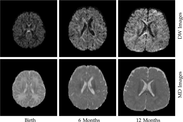
However, DMRI data suffers from low signal-to-noise-ratio (SNR), especially when the b-value is high. This is due to the fact that DMRI encodes the motion of water molecules via signal attenuation, which increases with diffusion weighting (i.e., b-value). The low SNR is aggravated in infant DMRI. The lack of myelin in restricting water mobility results in greater attenuation of the MR signal, causing lower SNR. Fig. 1 indicates that the quality of diffusion-weighted (DW) images is lower for earlier time points. The higher diffusivity closer to the perinatal period, as indicated by the mean diffusivity (MD) images, suggests greater water mobility.

Fig. 1: Data Quality.

Closer to the perinatal period, the quality of DW images (b = 1,500s/mm²) is lower due to signal attenuation associated with greater water mobility, as indicated by the mean diffusivity (MD) images.

Image quality can be improved by hardware methods, e.g., employing greater magnetic field strength [4] and averaging repeated scans [5]. However, these require either expensive hardware upgrades or prolonged acquisition times, which are prohibitive in clinical settings. Alternatively, software methods have been widely used for noise removal [6]–[13]. A particularly effective method is the non-local means (NLM) algorithm [6]–[9], which averages self-similar information gathered via neighborhood matching. However, when self-similar information does not recur, NLM can cause blurring and artifacts (see rare patch effect discussed in [14]–[17]). In DMRI, this typically happens in highly-curved white matter structures where the fiber orientations change significantly. This results in lower recurrence of signal patterns. Operating under such condition, NLM blurs diffusion signal profiles and aggravates partial volume effects.

In this paper, we propose a new neighborhood matching technique to overcome the limitations of NLM. DMRI acquires diffusion-weighted (DW) signals that are parameterized by both x-space (spatial domain) and q-space (wavevector domain). We encode the q-space sampling domain in a graph and view the DMRI signals in each voxel location as a function defined on the graph. Graph framelet transforms (GFTs), derived from the graph, are then applied to the function to extract features for neighborhood matching. Each GFT is used to extract features that correspond to a certain frequency subband of the spectrum obtained via graph spectral decomposition. This process is linear and is thus computationally efficient. Based on the GFT features, effective neighborhood matching can be carried out in x-q space, even for highly-curved white matter structures.

Based on the neighborhood matching technique described above, we proposed a method, called graph framelet matching (GFM), to remove the noise in DMRI data. GFM involves two major components, i.e., noise adaptation and noise reduction. Specifically, using the method presented in [18], we first transform the DMRI signals so that the noise in DMRI data follows a Gaussian distribution. This strategy can well adapt to various types of noise in modern multi-coil MR imaging, and simplify the task of noise reduction. We then employ the proposed neighborhood matching technique to local the redundant information in x-q space, and utilize the gathered information for the effective noise removal in an NLM framework. Thanks to the robust neighborhood matching technique, the information existing in highly-curved white matter structures can be effectively used for denoising. Extensive experiments on synthetic and real DMRI data demonstrate that GFM improves the denoising performance, both qualitatively and quantitatively.

A preliminary version of this work has been presented in a conference [19]. The method presented herein is a significantly improved version that considers various types of noise resulting from multi-coil MRI. More comprehensive evaluation is performed using synthetic and real data. The associated results, analyses, and discussions are new and not part of the conference publication.

The paper is organized as follows. In Section II, we give a detailed description of the proposed method. In Section III, we demonstrate the effectiveness of the proposed method with one synthetic dataset and two real datasets. In Section IV, we provide further discussions on this work. Finally, in Section V, we conclude this work.

II. Methods

In this section, we will describe our neighborhood matching technique and its application to DMRI denoising. First, we will introduce the theory of spectral graph convolution. Second, we will explain the details of GFTs, which are built upon the idea of graph convolution. Third, we will describe GFT-based neighborhood matching and its application to DMRI noise reduction. Finally, we will explain how noise removal can be performed for various types of noise in multi-coil MRI.

A. Spectral Graph Convolution

Unlike data uniformly sampled in the Euclidean space, convolution is less straightforward for irregularly-sampled data residing on manifolds. To achieve this, we introduce here the concept of spectral graph convolution.

We denote $\mathcal{G}:=\{\mathcal{E},\mathcal{V},w\}$ as a graph, where $\mathcal{V}:=\left\{v_k\in \mathcal{M}:k=0,\dots ,K-1\right\}$ is a set of points on the vertices, and a manifold $\mathcal{M},\mathcal{E}\subset \mathcal{V}\times \mathcal{V}$ is a set of edges relating $w:\mathcal{E}\mapsto {ℝ}^{+}$ is a weight function. Graph $\mathcal{G}$ is determined by an affinity matrix $\mathcal{A}$ which is symmetric with $w_{k,k^{\prime }}>0$ when two points k and, k′ are connected with each other. The graph Laplacian is defined is as $\mathcal{L}:=D-\mathcal{A}$ where $D:=\text{diag}\{d[1],d[2],\dots ,d[K]\}$ is a degree matrix with $d[k]:={\sum }_{k^{\prime }}{w}_{k,k^{\prime }}$. Denote by ${\left\{{\lambda }_k,u_k\right\}}_{k=0}^{K-1}$ the pairs of eigenvalues and eigenvectors of $\mathcal{L}$ with $0={\lambda }_0\le {\lambda }_1\le {\lambda }_2\le \dots \le {\lambda }_{K-1}={\lambda }_{\max }$. The eigenvectors form an orthonormal basis for all functions on the graph: $\langle u_k,u_{k^{\prime }}\rangle :=\sum _{l=0}^{K-1}{u}_k[l]u_{k^{\prime }}[l]={\delta }_{k,k^{\prime }}$. The Fourier transform of a function $f:\mathcal{V}\mapsto ℝ$ on the graph $\mathcal{G}$ is given by $\widehat{f}[k]:={\sum }_{l=0}^{K-1}f[l]u_k[l]=U^{\top }f$, where $U=\left[u_0,u_1,\dots ,u_{K-1}\right]$. The convolution of f with filter h on $\mathcal{G}$ is defined as

$$h\ast f=U\left(U^{\top }h\odot U^{\top }f\right)=U(\widehat{h}\odot \widehat{f})=U\text{diag}(\widehat{h})U^{\top }f,$$ (1)

where ⊙ represents a point-wise product. Such a convolution is called frequency filtering and $\widehat{h}$ is the transfer function of the filter. This is consistent with the classical convolution operator, judging from the fact that convolutions are by definition linear operators that diagonalize in the Fourier domain (see Convolution Theorem [20]). Designing a convolution filter thus amounts to determining the spectral multipliers $\{\widehat{h}[0],\widehat{h}[1],\dots ,\widehat{h}[K-1]\}$. While there are apparently many ways of doing so, we choose to achieve this using GFTs, which we will describe next.

B. Graph Framelet Transforms

GFT slices the frequency spectrum by using a set of masks $\left\{{\widehat{a}}_r(\cdot ):r=0,\dots ,R\right\}$, each corresponding to a subband, e.g., ${\widehat{a}}_0(\cdot )$ is a low-pass filter and the other masks, $\{{\widehat{a}}_r(\cdot ):0<r\le R\}$, are high-pass and band-pass filters. Information from the different subbands allows us to more accurately establish point-to-point correspondences of the nodes in the graph for improving denoising performance. As in [21], [22], we define GFTs for the function f as

$$\mathit{\alpha }:=\mathbf{W}f:=\left\{{\alpha }_{l,r}:=W_{l,r}f:(l,r)\in {\mathcal{B}}_{L,R}\right\},$$ (2)

where ${\mathcal{B}}_{L,R}:=\{(1,1),(1,2),\dots ,(1,R),(2,1),\dots ,(L,R)\}\cup \{(L,0)\}$ with maximum level L and

$$\widehat{W_{l,r}f}[k]:=\{\begin{array}{ll}\begin{array}{l}{\widehat{a}}_r\left({\gamma }^{-L+1}{\tilde{\lambda }}_k\right)\widehat{f}[k]\\ {\widehat{a}}_r\left({\gamma }^{-L+l}{\tilde{\lambda }}_k\right){\widehat{a}}_0\left({\gamma }^{-L+l-1}{\tilde{\lambda }}_k\right)\end{array}& l=1\\ \cdots {\widehat{a}}_0\left({\gamma }^{-L+1}{\tilde{\lambda }}_k\right)\widehat{f}[k]& 2\le l\le L,\end{array}$$ (3)

where ${\tilde{\lambda }}_k=\left({\lambda }_k/{\lambda }_{\max }\right)\pi$ and γ > 1 is a dilation factor. GFT is a linear transform and can be computed efficiently.

We reformulate (3) so that the transform can be performed without explicit spectral decomposition. Denoting $\mathcal{L}=U\text{Λ}{U}^{\top }$, where $\text{Λ}=\text{diag}\left\{{\lambda }_0,{\lambda }_1,\dots ,{\lambda }_{K-1}\right\}$, we have

$$W_{l,r}:=\{\begin{array}{ll}\begin{array}{l}U{\widehat{\text{Ω}}}_r\left({\gamma }^{-L+1}\widetilde{\text{Λ}}\right)U^{\top }\\ U{\widehat{\text{Ω}}}_r\left({\gamma }^{-L+l}\widetilde{\text{Λ}}\right){\widehat{\text{Ω}}}_0\left({\gamma }^{-L+l-1}\widetilde{\text{Λ}}\right)\end{array}& l=1\\ \cdots {\widehat{\text{Ω}}}_0\left({\gamma }^{-L+1}\widetilde{\text{Λ}}\right)U^{\top }& 2\le l\le L,\end{array}$$ (4)

where $\widetilde{\text{Λ}}=\text{diag}\left\{{\tilde{\lambda }}_0,{\tilde{\lambda }}_1,\dots ,{\tilde{\lambda }}_{K-1}\right\}$ and

$${\widehat{\text{Ω}}}_r(c\widetilde{\text{Λ}})=\text{diag}\left\{{\widehat{a}}_r\left(c{\tilde{\lambda }}_0\right),{\widehat{a}}_r\left(c{\tilde{\lambda }}_1\right),\dots ,{\widehat{a}}_r\left(c{\tilde{\lambda }}_{K-1}\right)\right\}.$$ (5)

All framelet masks, $\left\{{\widehat{a}}_r(\cdot )\right\}$ are generated based on the unitary extension principle (UEP) [22]. We show some examples of the masks in Table I. As in [22], [23], given a synthesis transform W^⊤, we can have

$${\mathbf{W}}^{\top }\mathit{\alpha }={\mathbf{W}}^{\top }\mathbf{W}f=\mathbf{I}f=f.$$ (6)

TABLE I:

Framelet masks.

Haar	Linear	Quadratic
${\widehat{a}}_0(\xi )=\cos \left(\frac{\xi }{2}\right)$ ${\widehat{a}}_1(\xi )=\sin \left(\frac{\xi }{2}\right)$	${\widehat{a}}_0(\xi )={\cos }^2\left(\frac{\xi }{2}\right)$ ${\widehat{a}}_1(\xi )=\frac{1}{\sqrt{2}}\sin (\xi )$ ${\widehat{a}}_2(\xi )={\sin }^2\left(\frac{\xi }{2}\right)$	${\widehat{a}}_0(\xi )={\cos }^3\left(\frac{\xi }{2}\right)$ ${\widehat{a}}_1(\xi )=\sqrt{3}\sin \left(\frac{\xi }{2}\right){\cos }^2\left(\frac{\xi }{2}\right)$ ${\widehat{a}}_2(\xi )=\sqrt{3}{\sin }^2\left(\frac{\xi }{2}\right)\cos \left(\frac{\xi }{2}\right)$ ${\widehat{a}}_3(\xi )={\sin }^3\left(\frac{\xi }{2}\right)$

C. Graph Representation of DMRI Data

We treat each point in q-space as a node in a graph and define the affinity weight between each pair of nodes using two Gaussian kernels, accounting for differences in gradient directions and diffusion weightings. Specifically, we define the affinity weight a_k,k^′ of two points k,k^′ in q-space as

$$a_{k,k^{\prime }}=\exp \left\{-\frac{1-{\left({\widehat{\mathbf{q}}}_k^{\top }{\widehat{\mathbf{q}}}_{k^{\prime }}\right)}^2}{2{\alpha }_{\text{p}}^2}\right\}\exp \left\{-\frac{{\left({\sqrt{b}}_k-{\sqrt{b}}_{k^{\prime }}\right)}^2}{2{\sigma }_{\text{p}}^2}\right\},$$ (7)

where ${\widehat{\mathbf{q}}}_k={\mathbf{q}}_k/\Vert {\mathbf{q}}_k\Vert$ is a normalized wavevector with ${\mathbf{q}}_k\in {ℝ}^3,b_k=t{\left|{\mathbf{q}}_k\right|}^2$ is the corresponding b-value with diffusion time t, α_p and σ_p are two parameters controlling the attenuations of two exponential functions, respectively. After computing the affinity weights between all the paired nodes in q-space, we then have the affinity matrix $\mathcal{A}:=\left(a_{k,k^{\prime }}\right)$ that encodes the q-space sampling geometric structure. Finally, the diffusion signals in each voxel are reformulated as a function defined on the graph.

D. Neighborhood Matching Using GFTs

We perform neighborhood matching based on the GFT features. A Gaussian function is employed to compute the similarity weight w_k;k^′ between two nodes k and k^′, defined as

$$w_{k;k^{\prime }}=\frac{1}{Z_k}\exp \left\{-\frac{{\Vert \varphi [k]-\varphi \left[k^{\prime }\right]\Vert }_2^2}{h_{\text{GFT}}^2\left(k,k^{\prime }\right)}\right\},$$ (8)

where Z_k is a normalization constant ensuring that the weights sum to one, $\varphi [k]:=\left\{{\alpha }_{l,r}[k]:(l,r)\in {\mathcal{B}}_{L,R}\right\}$ is the GFT coefficients for node k, and h_GFT(k,k^′) is a parameter controlling the attenuation of the exponential function. It can be observed that (8) encourages a large similarity weight for two nodes sharing similar GFT features.

Considering the variation of spatial location and b-value, we extend (8) to

$$\begin{gathered} w_{i,k;i^{\prime },k^{\prime }}= \\ \frac{1}{Z_{i,k}}\exp \left\{-\frac{{\Vert {\varphi }_i[k]-{\varphi }_{i^{\prime }}\left[k^{\prime }\right]\Vert }_2^2}{h_{\text{GFT}}^2\left(i,k;i^{\prime },k^{\prime }\right)}\right\}\exp \left\{-\frac{{\left({\sqrt{b}}_k-{\sqrt{b}}_{k^{\prime }}\right)}^2}{h_{\text{b}}^2}\right\}, \end{gathered}$$ (9)

where i,i^′ are two indices for different spatial locations, h_GFT(i,k;i^′, k^′) and h_b are two parameters controlling the bandwidths of the Gaussian kernels for differences in the GFT features and diffusion weightings. Referring to [24], we set

$$h_{\text{GFT}}\left(i,k;i^{\prime },k^{\prime }\right)=\sqrt{\beta \left({\widehat{\sigma }}_{i,k}^2+{\widehat{\sigma }}_{i^{\prime },k^{\prime }}^2\right)\left|{\varphi }_i[k]\right|},$$ (10)

where β is a constant, $\left|{\varphi }_i[k]\right|$ is the length of the feature vector, and ${\widehat{\sigma }}_{i,k}$ is the noise standard derivation estimated at point $(i,k)$. Similar to Eq. (10), we set $h_b=\sqrt{2}{\sigma }_{\text{b}}$, where σ_b is a scale parameter. The normalization constant, Z_i,k, in Eq. (9) is defined as

$$\begin{gathered} Z_{i,k}=\sum _{\left(i^{\prime },k^{\prime }\right)\in {\mathcal{V}}_{i,k}}\exp \left\{-\frac{{\Vert {\varphi }_i[k]-{\varphi }_{i^{\prime }}\left[k^{\prime }\right]\Vert }_2^2}{h_{\text{GFT}}^2\left(i,k;i^{\prime },k^{\prime }\right)}\right\} \\ \exp \left\{-\frac{{\left({\sqrt{b}}_k-{\sqrt{b}}_{k^{\prime }}\right)}^2}{h_{\text{b}}^2}\right\}, \end{gathered}$$ (11)

where $\mathcal{V}$_i,k is the search volume associated with an x-space search radius s and a q-space search angle θ.

E. Denoising via Neighborhood Matching in x-q Space

Similar to NLM [25], we estimate the underlying noise-free signal NLM(S)(x_i, q_k) using

$$\text{NLM}(S)\left({\mathbf{x}}_i,{\mathbf{q}}_k\right)=\sum _{\left(i^{\prime },k^{\prime }\right)\in {\mathcal{V}}_{i,k}}{w}_{i,k;i^{\prime },k^{\prime }}S\left({\mathbf{x}}_{i^{\prime }},{\mathbf{q}}_{k^{\prime }}\right),$$ (12)

where $S\left({\mathbf{x}}_{i^{\prime }},{\mathbf{q}}_{k^{\prime }}\right)$ is a diffusion signal associated with a spatial location ${\mathbf{x}}_{i^{\prime }}\in {ℝ}^3$ and a gradient q_k^′.

F. Adaptation to Various Types of Noise in Multi-Coil MRI

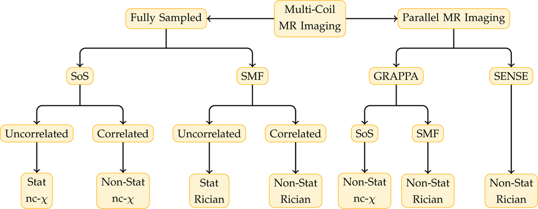
The classic NLM is designed to remove Gaussian noise and needs to be modified for the noncentral chi (nc-χ) distribution typical in modern multi-coil MRI [28]. The noise distribution of the composite magnitude signal (CMS) [28] given by modern multi-coil MRI techniques is dependent on how the k-space signal is sampled, how the magnitude signal is reconstructed, and how the coils are correlated. A summary of various types of noise for multi-coil MRI is shown in Fig. 2.

Fig. 2: Various Types of Noise in Multi-Coil MRI.

For fully-sampled k-space, sum of squares (SoS) and spatial matched filter (SMF) are common CMS reconstruction methods. For parallel MRI with subsampled k-space, sensitivity encoding (SENSE) [26] and generalized autocalibrating partially parallel acquisition (GRAPPA) [27] are well-known methods. The noise distribution is also influenced by correlation among coils. Multi-coil MRI produces signal with spatially stationary/non-stationary Rician/nc-χ noise distribution.

A number of methods [18], [29], [30] have been developed for dealing with the non-Gaussian nature of noise in MR images. For instance, Foi [29] proposed to determine a forward variance-stabilizing transformation to allow stationary Rician noise in MR magnitude images to be removed with filters designed for additive white Gaussian noise. The unbiased estimation of the true signal is obtained after denoising via a corresponding inverse variance-stabilizing transformation. This framework was extended in [30] for non-stationary Rician noise resulting from parallel MRI. Another promising method, presented in [31], uses nonlocal maximum likelihood method for estimating the underlying true signal from an MR image with spatially-varying noise.

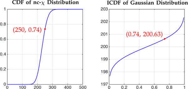
In this work, we adopt Koay et al.’s method [18] to transform a Rician/nc-χ signal to its Gaussian-distributed counterpart. This involves estimating the location parameter and Gaussian noise standard deviation of the nc-χ distribution and then performing signal transformation using the nc-χ cumulative distribution function (CDF) and the inverse Gaussian CDF [18], as illustrated in Fig. 3. Such signal transformation reduces the complexity of the denoising algorithm by not having to deal with the nc-χ nature of the noise [11], [18].

Fig. 3: Signal Transformation.

A nc-χ measurement S_nc−χ = 250 is mapped to the corresponding Gaussian measurement S_Gaussian = 200.63 using common probability P = 0.74.

The estimation of noise standard derivation is key to accurate signal transformation. For spatially stationary noise, the noise standard derivation can be estimated from the image background using a method called probabilistic identification and estimation of noise (PIESNO) [32] or from doubly-acquired images using the method described in [33]. For spatially non-stationary noise, a number of noise estimation methods [11], [30], [34]–[38] have been proposed. For instance, inspired by the work presented in [39], Veraart et al. [40] estimated the spatially-varying noise in DMRI data by using the median absolute deviation estimator in the wavelet domain and Koay’s inversion technique [41]. The resulting noise map was then used for improving the estimation accuracy of diffusion MRI parameters. Manjón et al. [35] suggested using principle component analysis (PCA) for noise estimation and reduction in DMRI. Veraart et al. [36] proposed a method, called Marchenko-Pastur PCA (MP-PCA), that identifies the noise-only principal components automatically based on random matrix theory. In this work, we use MP-PCA [36] for estimating the spatially-varying noise level.

III. Experiments

A. Datasets

We evaluated the proposed method using one synthetic dataset and two real datasets. All real data were acquired at the Biomedical Research Imaging Center (BRIC) of the University of North Carolina (UNC) at Chapel Hill. Informed written consent was obtained from the all the subjects and the experimental protocols were approved by the Institutional Review Board of UNC School of Medicine. The study was carried out in accordance with the approved guidelines.

1). Synthetic Data:

For quantitative evaluations, we generated a synthetic multi-shell dataset using phantomαs [42]. The fiber geometric setting was based on the description file used in the ISBI 2013 HARDI challenge¹. Consistent with the infant data described in Section III-A3, the synthetic data were generated using b = 700,1500,3000s/mm² with a total of 144 non-collinear gradient directions. Image dimensions are 55 × 55 × 55 with 1.5 × 1.5 × 1.5mm² resolution.

To evaluate the effect of noise removal of our method, the ground truth data was added with stationary and non-stationary nc-χ noise with different noise levels (3%, 5%, 7%, and 9%) and numbers of channels (1, 4, 8, and 12). Note that the nc-χ distribution with one channel is equivalent to a Rician distribution. The nc-χ noise is simulated using

$$Y_N=\sqrt{{\left({\mu }_N+X(1)\right)}^2+\sum _{k=2}^{2N}{[X(k)]}^2,}$$ (13)

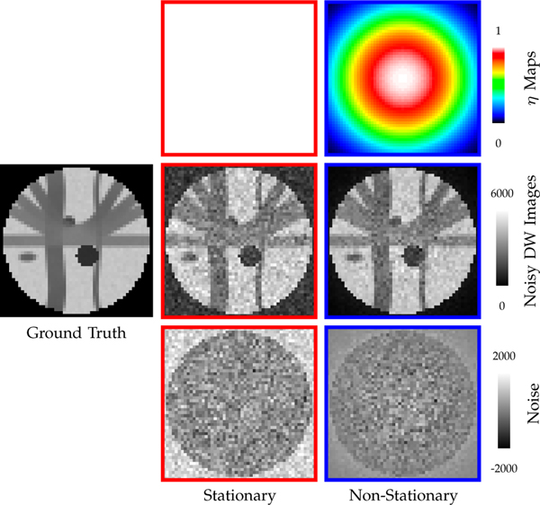
where N is the number of channels, Y_N is the noisy signal, μ_N is the true signal, and $X(k)\sim \mathcal{N}(0,\eta \sigma )$ is a random variable following a Gaussian distribution with standard derivation ησ. We set σ to p percentages of the maximum signal value v, i.e., σ = v(p/100), and change p to simulate different noise levels [24]. We change η to simulate spatial stationary and non-stationary noise. Specifically, as illustrated in Fig. 4, a constant η map leads to stationary noise, whereas a spatially varying η map leads to non-stationary noise.

Fig. 4: Noise Simulation.

5% 4-channel nc-χ noise with spatially constant and varying η maps for b = 700s/mm².

2). Repetitively-Acquired Data:

We acquired the brain DMRI data of an adult 25 times using a Siemens 3T Magnetom Prisma MR scanner with the following imaging protocol: b = 3000s/mm², 42 gradient directions, 140 × 140 imaging matrix, voxel size 1.5 × 1.5 × 1.5 mm³, TE=89ms, TR=2,513ms, 32 receiver coils. We performed signal transformation [43] and eddy correction [44] for each dataset. The 25 processed datasets were averaged to form a gold standard with improved SNR for evaluation purposes.

3). Infant Data:

This dataset consists of a set of longitudinal infant brain DMRI data covering three time points, i.e., 0 month, 6 months, and 12 months. All data were from the Baby Connectome Project (BCP) [45] and were acquired using the Siemens 3T Magnetom Prisma MR scanner with the following imaging protocol: 140 × 140 imaging matrix, 1.5 × 1.5 × 1.5 mm³ resolution, TE=88ms, TR=2,365ms, 32-channel receiver coil. Gradient directions and b-values were identical to the synthetic data. CMS reconstruction was performed using SENSE1 [46], resulting in non-stationary Rician noise distribution.

B. Parameter Settings

The parameters of GFM can be divided into two categorizes, i.e., parameters for GFT feature computation and x-q space non-local denoising. For the first category, we used the quadratic masks and set the decomposition level to L = 4. We used the low-frequency subbands since they are relatively unaffected by noise. The parameters in the second category were as follows:

1. Constant β: It is suggested in [24] to set β = 1. However, based on the theory of kernel regression, decreasing the bandwidth will reduce bias when the sample size is large [47]. In our case, the sample size is significantly increased since information in the joint x-q space is considered. Therefore, we set β = 0.1.

2. Tuning parameter σ_b: Based on the diffusion gradients described in Section III-A3, we computed the typical value for $\left|\sqrt{b_k}-\sqrt{b_l}\right|$, which is $\sqrt{1500}-\sqrt{700}\approx 12$ Therefore, we set ${\sigma }_{\text{b}}=12/2=6$.

3. x-space search radius s: Coupé et al. suggested to set s = 5, corresponding too 5mm in physical distance) [24]. We set s = 2 since the voxel size of DW images is typical two times that of structural MR images in each physical dimension.

4. q-space search angle θ: We set θ = 2 × 15° = 30° based on the average angular separation of the gradient directions (15°).

5. Tuning parameter α_p: Based on the same average angular separation, we set ${\alpha }_{\text{p}}=\sqrt{1-{\cos }^2\left({15}^{\circ }\right)}\approx 0.26$.

6. Tuning parameter σ_p: Our data are all shell-sampled. Therefore, we set σ_p to a small value, 0.1, for greater localization.

C. Methods for Comparison

We compared GFM with the following methods:

1. Adaptive non-local means (ANLM): ANLM [34] is an extension of the NLM algorithm, which removes spatially non-stationary noise. Based on [34], we set the patch radius to 1.

2. Non-local spatial and angular matching (NLSAM): NLSAM [11] consists of three major steps, i.e., (i) Signal transformation so that the signals are Gaussian distributed; (ii) 4D block construction by considering diffusion-weighted images within an angular neighborhood; (iii) Noise removal using sparse representation. Based on [11], we set the patch radius to 1 and use 5 angular neighbours.

3. x-q space non-local means (XQ-NLM): XQ-NLM defines spherical patches in q-space. After mapping the spherical patch to a 2D disk, rotation-invariant features are computed using polar complex exponential transform (PCET) [48]. The resulting features are then used in x-q space patch matching. Finally, the signal is denoised through weighted averaging of self-similar information. Based on [12], we set the maximum order of PCET to 4. Other parameters are consistent with GFM and also based on the default values suggested in [12].

For fair comparison, we used the non-stationary noise field estimated by MP-PCA for ANLM, NLSAM, XQ-NLM, and GFM. For stationary noise, the noise standard deviation was determined using PIESNO [32].

D. Methods of Evaluation

Quantitative and qualitative evaluations were performed:

1. Peak signal-to-noise ratio (PNSR): We used PSNR as the metric for performance evaluation. PSNR is defined

   $$\text{PSNR}=20{\log }_{10}\frac{\text{MAX}}{\text{RMSE}},$$ (14)

   where RMSE is the root mean square error computed between the denoised image and the ground truth noise free image, MAX is the maximum signal value.

2. Generalized fractional anisotropy (GFA) image: We computed the GFA image [49] using Dipy [50] based on the method described in [51].

3. Mean absolute difference (MAD): We computed the absolute difference (AD) map between each GFA image G and the gold standard G_True. The MAD value was calculated by averaging across voxels in a brain region. Mathematically, MAD is defined as $\frac{1}{|\text{Ω}|}{\sum }_{i\in \text{Ω}}\mid G_{\text{True}}(i)-G(i)\mid$, where G(i) and $G_{\text{True}}(i)$ are the GFA values at location i in the brain region Ω.

4. RMSE map: Pixelwise accuracy was evaluated using the RMSE computed between the denoised signal vector at each voxel location with respect to the ground truth.

5. Residual map: We computed the residual map by subtracting denoised DW image from its noisy version. An ideal residual map should show noise and contain as little structural information as possible.

6. Fiber orientations: We evaluated the fiber orientation distribution functions (ODFs) [52] and the local minima [53].

7. Probability of false fiber detection (PFFD): We computed PFFD [54] using

   $$\frac{\left|P_{\text{True}}-P_{\text{Estimated}}\right|}{P_{\text{True}}}\times 100\text{\%,}$$ (15)

   where P_True and P_Estimated are respectively the numbers of ground truth peaks and estimated peaks in a voxel.
8. Average angular error (AAE): We utilized AAE [54] to measure the angular accuracy of fiber orientations. AAE is defined as the average value of the angular errors computed for all ground true fiber peaks in one voxel. The associated angular error is defined as

   $$\frac{180}{\pi }\arccos \left(\left|{\mathbf{d}}_{\text{True}}\cdot {\mathbf{d}}_{\text{Estimated}}\right|\right),$$ (16)

   where d_True and d_Estimated are the ground truth peak direction and its closest estimation, respectively. We use to denote the dot product.

E. Results

1). Neighborhood Matching:

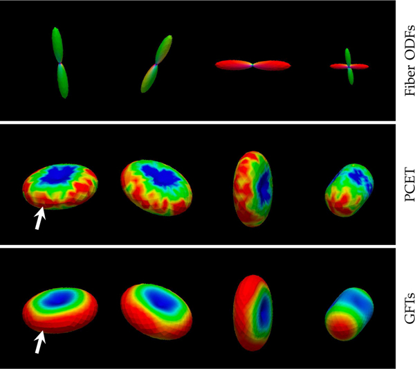
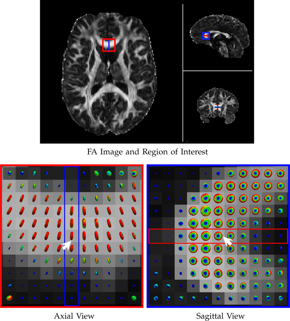
We first evaluated the neighborhood matching performance of GFTs with respect to PCET [48], which is used in XQ-NLM [12]. The results, shown in Fig. 5, indicate that neighborhood matching with GFTs is more accurate and more robust to noise than PCET. Note that the matching is not affected by the orientation of the signal profiles. Fig. 6 shows the matching results in the corpus callosum region of a real dataset, clearly demonstrating the effectiveness of the matching mechanism in curved white matter structures.

Fig. 5: Neighborhood Matching.

Neighborhood matching is performed in the presence of noise with respect to the point marked by the white arrow. Warm colors indicate greater agreement; cool colors indicate otherwise. Matching performance is significantly better in the case of GFT features than PCET features.

Fig. 6: Neighborhood Matching in Real Data.

Similar to Fig. 5, but showing the neighborhood matching results in the corpus callosum of a real dataset. The results in the marked region are shown in axial and sagittal views.

2). Synthetic Data:

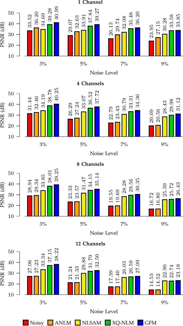
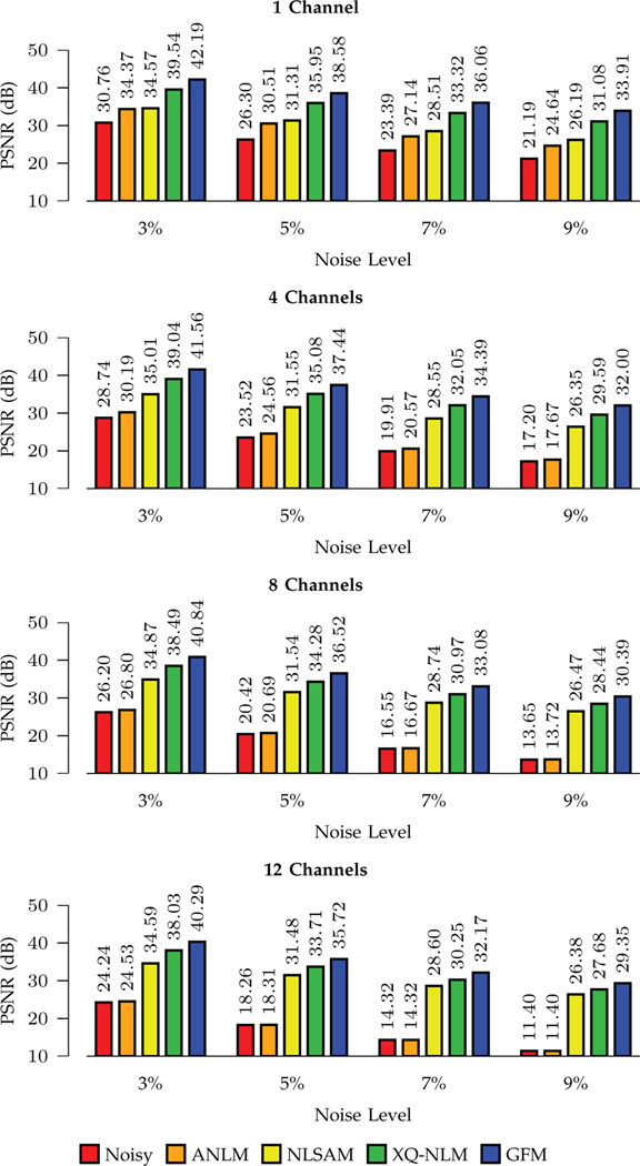
We show the PSNR results shown in Figs. 7 and 8. For stationary noise, GFM performs best for all noise levels and channel numbers. Compared with the second best method, XQ-NLM, GFM yields a largest improvement of 2.8dB when the noise level is 9% (one channel). For non-stationary noise, conclusions consistent with Fig. 7 can be drawn from Fig. 8, indicating that GFM performs best among all methods.

Fig. 7: PSNR Comparison – Stationary Noise.

Denoising performance for different noise levels and channel numbers.

Fig. 8: PSNR Comparison – Non-Stationary Noise.

Denoising performance for different noise levels and channel numbers.

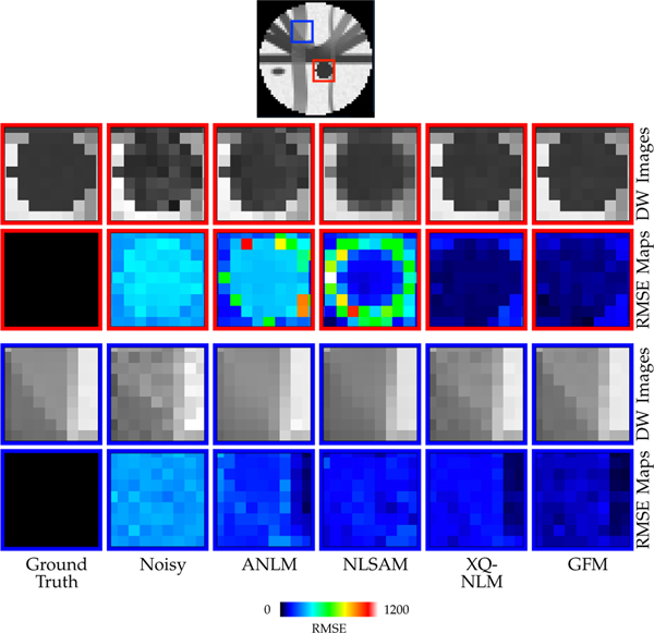
Fig. 9 shows the regional close-up views of DW images and RMSE maps. From the region marked by the red rectangle, it can be observed that XQ-NLM and GFM perform best in terms of edge preservation. In contrast, ANLM and NLSAM blur boundaries and result in higher RMSE values. The advantages of GFM over XQ-NLM can be clearly observed in the region marked by the blue rectangle, with GFM producing clearer boundaries and lower RMSE values than XQ-NLM. The blurring effects of ANLM over NLSAM can also be observed in this region.

Fig. 9: DW Images and RMSE Maps.

Boundary effects of various smoothing algorithms.

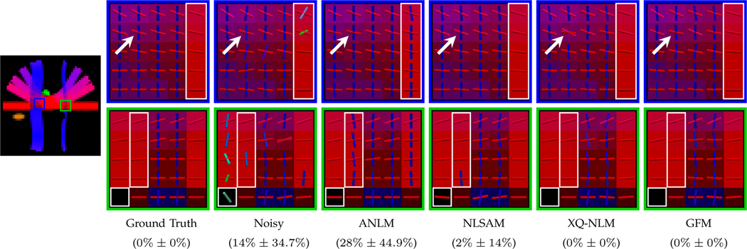
The fiber peaks, shown as ‘sticks’ in in Fig. 10, indicate that GFM is able to produce clean fiber peaks similar to the ground truth. In regions marked by rectangles, spurious fiber peaks are produced by ANLM and NLSAM due to partial volume effects from blurring. In the region marked by the arrow, a missing fiber peak is observed in the result given by XQ-NLM. In contrast, GFM produces correct fiber peaks and avoids such error. For quantitative evaluation, we show the PFFD values of the regions of interest at the bottom of Fig. 10. It can be observed that GFM and XQ-NLM correctly recover all fiber orientations without introducing any false positives or false negatives. In contrast, ANLM and NLSAM give unsatisfactory results by causing spurious peaks. Moreover, GFM gives an AAE of (3.8° ± 2.1°) compared with (4.1° ± 5.1°) given by XQ-NLM, indicating that GFM improves angular accuracy.

Fig. 10: Fiber Peaks.

Local maxima of ODFs shown as sticks. The PFFD means and standard deviations for the regions of interest are shown at the bottom.

3). Repetitively-Acquired Data:

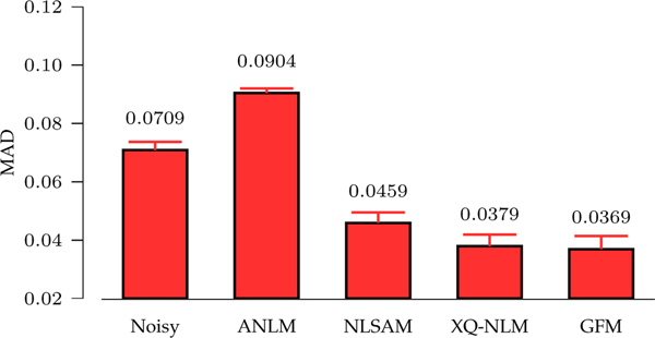
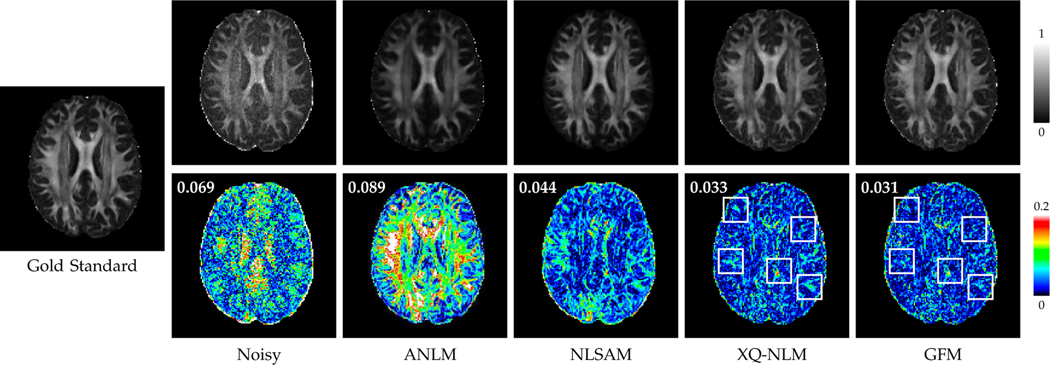
Fig. 11 indicates that GFM gives the lowest GFA mean MAD values, computed over the 25 datasets, with respect to the gold standard. Fig. 12 shows the GFA images and associated GFA AD maps of one dataset. Compared with ANLM and NLSAM, XQ-NLM and GFM significantly reduce the AD values. Furthermore, the improvement of GFM over XQ-NLM is clearly observed in the regions marked by white rectangles. Overall, GFM give a GFA image with the best quality and lowest MAD value. The superior performance of GFM can be attributed to the fact that GFM is able to preserve edges while effectively remove noise. As shown in the synthetic data experiments, ANLM and NLSAM over-smooth DW images. Smoothing also blurs diffusion signal profile in q-space, lowering the GFA value.

Fig. 11: GFA MAD Comparison.

For each of 25 repetitively-acquired datasets, we computed the MAD values for the GFA images given by the different methods. The means and standard deviations computed across the 25 datasets are shown.

Fig. 12: GFA Images and AD Maps.

GFA images and the associated AD maps. GFM yields lower AD values than XQ-NLM, especially in the regions marked with rectangles. MAD values are shown in the top left corners of AD maps.

4). Infant Data:

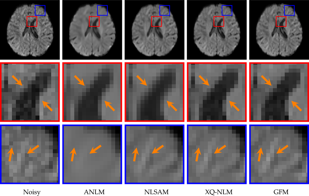
Since our method gives consistent performance for all time points, we only report the results for the 8-month subject here. Please refer to the supplementary materials for the results of all time points. Fig. 13 indicates that both XQ-NLM and GFM are effective in preserving structural information while removing noise. In contrast, the boundaries between white matter and the ventricles are blurred by ANLM and NLSAM. Moreover, the regions marked by blue rectangles in Fig. 13 indicate that GFM is better at preserving edges than XQ-NLM.

Fig. 13: DW Images.

Edge-preserving performance of various denoising algorithms. The DMRI data of the 6-month subject was used in the evaluation.

Fig. 14 shows the residual maps for different methods. In contrast to ANLM and NLSAM, GFM and XQ-NLM result in little structural information in the residual maps, confirming that the edge-preserving effects observed in Fig. 13.

Fig. 14: Residual Maps.

Evaluation of whether structural information is removed during denoising.

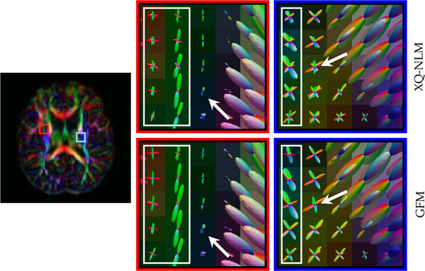
We further investigated the influence of denoising on fiber ODFs. The results, shown in Fig. 15, indicate that GFM yields fiber ODFs that are clearer and more coherent, compared with XQ-NLM.

Fig. 15: Fiber ODFs.

Fiber ODF comparison between XQ-NLM and GFM at different time points.

These experiments demonstrate that GFM is effective in removing noise in infant DMRI, which can be beneficial for studies on brain development [55], [56].

IV. Discussion

The edge-preserving property of GFM can be attributed to the nature of the neighborhood matching framework, which can be summarized in three aspects:

• Rich characterization of signal pattern: GFTs decompose the signal into multiple frequency subbands and is thus able to provide a rich characterization of signal patterns. As demonstrated in Fig. 5 and 6, GFTs significantly improve the accuracy of neighborhood matching.

• Rotation-invariance: Since the graph Laplacian used to generate GFTs is agnostic to orientation, GFTs are rotation-invariant. The rotation-invariance of property GFTs provides a good basis for neighborhood matching in structures with different orientations.

• Linear operation: GFTs are linear operations. This significantly simplifies the implementation of GFTs and reduces computation times.

GFM is computationally efficiency, as verified by Table II, where we show the computation times of different methods when for one randomly selected dataset from the repetitively-acquired data described in Section III-A2. GFM is about two times faster than XQ-NLM, the second best performing method. We implemented ANLM, XQ-NLM, and GFM using C++ based on the Insight Segmentation and Registration Toolkit (ITK) ². NLSAM was compiled from source code³. Evaluation was based on a computer with a four-core 2.9GHz Intel Core i7 CPU.

TABLE II:

Comparison of computation times.

	ANLM	NLSAM	XQ-NLM	GFM
Time (mins)	33.2	332.2	115.5	49.4

While effective, GFM has several limitations. First, GFM requires a significant amount of memory for storing the GFT features. This can be resolved by performing noise reduction in local regions and then combining the results. Second, GFM, while faster than competing methods, is still not fast enough for real-time applications. Speed can be improved by using the neighborhood preselection strategy described in [34]. Third, unbiased noise reduction is still challenging for some noise distributions, e.g., the spatially-varying nc-χ noise distribution resulting from GRAPPA with SoS reconstruction [28]. Signal transformation cannot be properly performed due to the difficulty in estimating the parameters of the noise distribution.

The proposed method provides a general framework for performing neighborhood matching of structures that are orientationally different. We can apply our method to improve algorithms that rely on neighborhood matching; for instance, super-resolution [57], [58], atlas building [59]–[61], ODF estimation [62], [63], voxel-based morphometry [64], etc.

V. Conclusion

We have introduced a neighborhood matching technique for curved domains and applied it to the noise reduction of DMRI data. Extensive experiments were performed using synthetic data, repetitively-acquired data, and infant data. The experimental results demonstrate that our method, GFM, preserves edges while removing noise, significantly reducing noise-induced artifacts in derived diffusion quantities. The proposed method outperforms various state-of-the-art methods, both qualitatively and quantitatively.

References

- [1].Cascio CJ, Gerig G, and Piven J, “Diffusion tensor imaging: application to the study of the developing brain,” Journal of the American Academy of Child & Adolescent Psychiatry, vol. 46, no. 2, pp. 213–223, 2007. [DOI] [PubMed] [Google Scholar]
- [2].Yap P-T, Fan Y, Chen Y, Gilmore J, Lin W, and Shen D, “Development trends of white matter connectivity in the first years of life,” PLoS ONE, vol. 6, no. 9, p. e24678, 2011. [DOI] [PMC free article] [PubMed] [Google Scholar]
- [3].Travers BG, Adluru N, Ennis C, Tromp DP, Destiche D, Doran S, Bigler ED, Lange N, Lainhart JE, and Alexander AL, “Diffusion tensor imaging in autism spectrum disorder: a review,” Autism Research, vol. 5, no. 5, pp. 289–313, 2012. [DOI] [PMC free article] [PubMed] [Google Scholar]
- [4].Gilmore JH, Zhai G, Wilber K, Smith JK, Lin W, and Gerig G, “3 tesla magnetic resonance imaging of the brain in newborns,” Psychiatry Research: Neuroimaging, vol. 132, no. 1, pp. 81–85, 2004. [DOI] [PubMed] [Google Scholar]
- [5].Seghier ML, Lazeyras F, Zimine S, Saudan-Frei S, Safran AB, and Huppi PS, “Visual recovery after perinatal stroke evidenced by functional and diffusion MRI: Case report,” BMC neurology, vol. 5, no. 1, p. 17, 2005. [DOI] [PMC free article] [PubMed] [Google Scholar]
- [6].Wiest-Daesslé N, Prima S, Coupé P, Morrissey SP, and Barillot C, “Non-local means variants for denoising of diffusion-weighted and diffusion tensor MRI,” in Medical Image Computing and Computer-Assisted Intervention–MICCAI 2007. Springer, 2007, pp. 344–351. [DOI] [PMC free article] [PubMed] [Google Scholar]
- [7].Descoteaux M, Wiest-Daesslé N, Prima S, Barillot C, and Dériche R, “Impact of Rician adapted non-local means filtering on HARDI,” in Medical Image Computing and Computer-Assisted Intervention–MICCAI 2008. Springer, 2008, pp. 122–130. [DOI] [PubMed] [Google Scholar]
- [8].Yap P-T, An H, Chen Y, and Shen D, “Uncertainty estimation in diffusion MRI using the nonlocal bootstrap,” IEEE Transactions on Medical Imaging, vol. 33, no. 8, pp. 1627–1640, 2014. [DOI] [PMC free article] [PubMed] [Google Scholar]
- [9].Chen G, Zhang P, Wu Y, Shen D, and Yap P-T, “Denoising magnetic resonance images using collaborative non-local means,” Neurocomputing, vol. 177, pp. 215–227, 2016. [DOI] [PMC free article] [PubMed] [Google Scholar]
- [10].Manjón JV, Coupé P, Martí-Bonmatí L, Collins DL, and Robles M, “Adaptive non-local means denoising of MR images with spatially varying noise levels,” Journal of Magnetic Resonance Imaging, vol. 31, no. 1, pp. 192–203, 2010. [DOI] [PubMed] [Google Scholar]
- [11].St-Jean S, Coupe P, and Descoteaux M, “Non local spatial and angular matching: Enabling higher spatial resolution diffusion MRI datasets through adaptive denoising,” Medical Image Analysis, vol. 32, pp. 115–130, 2016. [DOI] [PubMed] [Google Scholar]
- [12].Chen G, Wu Y, Shen D, and Yap P-T, “Noise reduction in diffusion MRI using non-local self-similar information in joint x-q space,” Medical Image Analysis, vol. 53, pp. 79–94, 2019. [DOI] [PMC free article] [PubMed] [Google Scholar]
- [13].Chen G, Zhang J, Zhang Y, Dong B, Shen D, and Yap P-T, “Multichannel framelet denoising of diffusion-weighted images,” PloS one, vol. 14, no. 2, p. e0211621, 2019. [DOI] [PMC free article] [PubMed] [Google Scholar]
- [14].Duval V, Aujol J-F, and Gousseau Y, “A bias-variance approach for the nonlocal means,” SIAM Journal on Imaging Sciences, vol. 4, no. 2, pp. 760–788, 2011. [Google Scholar]
- [15].Deledalle C-A, Duval V, and Salmon J, “Non-local methods with shape-adaptive patches (NLM-SAP),” Journal of Mathematical Imaging and Vision, vol. 43, no. 2, pp. 103–120, 2012. [Google Scholar]
- [16].Salmon J. and Strozecki Y, “Patch reprojections for non-local methods,” Signal Processing, vol. 92, no. 2, pp. 477–489, 2012. [Google Scholar]
- [17].Foi A. and Boracchi G, “Foveated nonlocal self-similarity,” International Journal of Computer Vision, vol. 120, no. 1, pp. 78–110, 2016. [Google Scholar]
- [18].Koay CG, Özarslan E, and Basser PJ, “A signal transformational¨ framework for breaking the noise floor and its applications in MRI,” Journal of Magnetic Resonance, vol. 197, no. 2, pp. 108–119, 2009. [DOI] [PMC free article] [PubMed] [Google Scholar]
- [19].Chen G, Dong B, Zhang Y, Shen D, and Yap P-T, “Neighborhood matching for curved domains with application to denoising in diffusion MRI,” in International Conference on Medical Image Computing and Computer-Assisted Intervention. Springer, 2017, pp. 629–637. [DOI] [PMC free article] [PubMed] [Google Scholar]
- [20].Mallat S, A Wavelet Tour of Signal Processing: The Sparse Way, third edition ed. Academic Press, 2008. [Google Scholar]
- [21].Hammond DK, Vandergheynst P, and Gribonval R, “Wavelets on graphs via spectral graph theory,” Applied and Computational Harmonic Analysis, vol. 30, no. 2, pp. 129–150, 2011. [Google Scholar]
- [22].Dong B, “Sparse representation on graphs by tight wavelet frames and applications,” Applied and Computational Harmonic Analysis, vol. 42, no. 3, pp. 452–479, 2017. [Google Scholar]
- [23].Ron A. and Shen Z, “Affine systems in L2(ℝd): The analysis of the analysis operator,” Journal of Functional Analysis, vol. 148, no. 2, pp. 408–447, 1997. [Google Scholar]
- [24].Coupé P, Yger P, Prima S, Hellier P, Kervrann C, and Barillot C, “An optimized blockwise nonlocal means denoising filter for 3-D magnetic resonance images,” IEEE Transactions on Medical Imaging, vol. 27, no. 4, pp. 425–441, 2008. [DOI] [PMC free article] [PubMed] [Google Scholar]
- [25].Buades A, Coll B, and Morel J-M, “A review of image denoising algorithms, with a new one,” Multiscale Modeling & Simulation, vol. 4, no. 2, pp. 490–530, 2005. [Google Scholar]
- [26].Pruessmann KP, Weiger M, Scheidegger MB, Boesiger P. et al. , “SENSE: Sensitivity encoding for fast MRI,” Magnetic Resonance in Medicine, vol. 42, no. 5, pp. 952–962, 1999. [PubMed] [Google Scholar]
- [27].Griswold MA, Jakob PM, Heidemann RM, Nittka M, Jellus V, Wang J, Kiefer B, and Haase A, “Generalized autocalibrating partially parallel acquisitions (GRAPPA),” Magnetic Resonance in Medicine, vol. 47, no. 6, pp. 1202–1210, 2002. [DOI] [PubMed] [Google Scholar]
- [28].Aja-Fernández S. and Vegas-Sánchez-Ferrero G, Statistical Analysis of Noise in MRI. Springer, 2016. [Google Scholar]
- [29].Foi A, “Noise estimation and removal in MR imaging: The variance-stabilization approach,” in International Symposium on Biomedical Imaging (ISBI), March 2011, pp. 1809–1814.
- [30].Pieciak T, Aja-Fernández S, and Vegas-Sánchez-Ferrero G, “Non-stationary Rician noise estimation in parallel MRI using a single image: a variance-stabilizing approach,” IEEE Transactions on Pattern Analysis and Machine Intelligence, vol. 39, no. 10, pp. 2015–2029, 2017. [DOI] [PubMed] [Google Scholar]
- [31].Rajan J, Veraart J, Van Audekerke J, Verhoye M, and Sijbers J, “Nonlocal maximum likelihood estimation method for denoising multiplecoil magnetic resonance images,” Magnetic Resonance Imaging, vol. 30, no. 10, pp. 1512–1518, 2012. [DOI] [PubMed] [Google Scholar]
- [32].Koay CG, Özarslan E, and Pierpaoli C, “Probabilistic identification¨ and estimation of noise (PIESNO): A self-consistent approach and its applications in MRI,” Journal of Magnetic Resonance, vol. 199, no. 1, pp. 94–103, 2009. [DOI] [PMC free article] [PubMed] [Google Scholar]
- [33].Sijbers J, Den Dekker A, Van Audekerke J, Verhoye M, and Van Dyck D, “Estimation of the noise in magnitude MR images,” Magnetic Resonance Imaging, vol. 16, no. 1, pp. 87–90, 1998. [DOI] [PubMed] [Google Scholar]
- [34].Manjón JV, Coupé P, Martí-Bonmatí L, Collins DL, and Robles M, “Adaptive non-local means denoising of MR images with spatially varying noise levels,” Journal of Magnetic Resonance Imaging, vol. 31, no. 1, pp. 192–203, 2010. [DOI] [PubMed] [Google Scholar]
- [35].Manjón JV, Coupé P, Concha L, Buades A, Collins DL, and Robles M, “Diffusion weighted image denoising using overcomplete local PCA,” PloS one, vol. 8, no. 9, p. e73021, 2013. [DOI] [PMC free article] [PubMed] [Google Scholar]
- [36].Veraart J, Fieremans E, and Novikov DS, “Diffusion MRI noise mapping using random matrix theory,” Magnetic resonance in medicine, vol. 76, no. 5, pp. 1582–1593, 2016. [DOI] [PMC free article] [PubMed] [Google Scholar]
- [37].Rajan J, Poot D, Juntu J, and Sijbers J, “Noise measurement from magnitude MRI using local estimates of variance and skewness,” Physics in Medicine and Biology, vol. 55, no. 16, p. N441, 2010. [DOI] [PubMed] [Google Scholar]
- [38].Aja-Fernández S, Pieciak T, Vegas-Sánchez-Ferrero G. et al. , “Spatially variant noise estimation in MRI: A homomorphic approach,” Medical Image Analysis, vol. 20, no. 1, pp. 184–197, 2015. [DOI] [PubMed] [Google Scholar]
- [39].Coupé P, Manjón JV, Gedamu E, Arnold D, Robles M, and Collins DL, “Robust Rician noise estimation for MR images,” Medical Image Analysis, vol. 14, no. 4, pp. 483–493, 2010. [DOI] [PubMed] [Google Scholar]
- [40].Veraart J, Rajan J, Peeters RR, Leemans A, Sunaert S, and Sijbers J, “Comprehensive framework for accurate diffusion MRI parameter estimation,” Magnetic Resonance in Medicine, vol. 70, no. 4, pp. 972–984, 2013. [DOI] [PubMed] [Google Scholar]
- [41].Koay CG and Basser PJ, “Analytically exact correction scheme for signal extraction from noisy magnitude MR signals,” Journal of Magnetic Resonance, vol. 179, pp. 317–322, 2006. [DOI] [PubMed] [Google Scholar]
- [42].Caruyer E, Daducci A, Descoteaux M, Houde J-C, Thiran J-P, and Verma R, “Phantomas: A flexible software library to simulate diffusion MR phantoms,” in ISMRM, 2014.
- [43].Eichner C, Cauley SF, Cohen-Adad J, Möller HE, Turner R, Setsompop K, and Wald LL, “Real diffusion-weighted MRI enabling true signal averaging and increased diffusion contrast,” NeuroImage, vol. 122, pp. 373–384, 2015. [DOI] [PMC free article] [PubMed] [Google Scholar]
- [44].Andersson JL and Sotiropoulos SN, “An integrated approach to correction for off-resonance effects and subject movement in diffusion MR imaging,” NeuroImage, vol. 125, pp. 1063–1078, 2016. [DOI] [PMC free article] [PubMed] [Google Scholar]
- [45].Howell BR, Styner MA, Gao W, Yap P-T, Wang L, Baluyot K, Yacoub E, Chen G, Potts T, Salzwedel A. et al. , “The UNC/UMN baby connectome project (BCP): an overview of the study design and protocol development,” NeuroImage, 2018. [DOI] [PMC free article] [PubMed]
- [46].Sotiropoulos SN, Moeller S, Jbabdi S, Xu J, Andersson JL, Auerbach EJ, Yacoub E, Feinberg D, Setsompop K, Wald LL, Behrens TEJ, Ugurbil K, and Lenglet C, “Effects of image reconstruction on fiber orientation mapping from multichannel diffusion MRI: Reducing the noise floor using SENSE,” Magnetic Resonance in Medicine, vol. 70, pp. 1682–1689, 2013. [DOI] [PMC free article] [PubMed] [Google Scholar]
- [47].Silverman B, Density Estimation for Statistics and Data Analysis, ser. Monographs on Statistics and Applied Probablilty. Chapman and Hall, 1998. [Google Scholar]
- [48].Yap P-T, Jiang X, and Kot AC, “Two-dimensional polar harmonic transforms for invariant image representation,” IEEE Transactions on Pattern Analysis and Machine Intelligence, vol. 32, no. 7, pp. 1259–1270, 2010. [DOI] [PubMed] [Google Scholar]
- [49].Tuch DS, “Q-ball imaging,” Magnetic Resonance in Medicine, vol. 52, no. 6, pp. 1358–1372, 2004. [DOI] [PubMed] [Google Scholar]
- [50].Garyfallidis E, Brett M, Amirbekian B, Rokem A, Van Der Walt S, Descoteaux M, and Nimmo-Smith I, “Dipy, a library for the analysis of diffusion MRI data,” Frontiers in neuroinformatics, vol. 8, p. 8, 2014. [DOI] [PMC free article] [PubMed] [Google Scholar]
- [51].Aganj I, Lenglet C, Sapiro G, Yacoub E, Ugurbil K, and Harel N, “Reconstruction of the orientation distribution function in single-and multiple-shell q-ball imaging within constant solid angle,” Magnetic Resonance in Medicine, vol. 64, no. 2, pp. 554–566, 2010. [DOI] [PMC free article] [PubMed] [Google Scholar]
- [52].Yap PT, Zhang Y, and Shen D, “Multi-tissue decomposition of diffusion MRI signals via ℓ0 sparse-group estimation,” IEEE Transactions on Image Processing, vol. 25, no. 9, pp. 4340–4353, 2016. [DOI] [PMC free article] [PubMed] [Google Scholar]
- [53].Yap P-T and Shen D, “Spatial transformation of DWI data using nonnegative sparse representation,” IEEE Transactions on Medical Imaging, vol. 31, no. 11, pp. 2035–2049, 2012. [DOI] [PMC free article] [PubMed] [Google Scholar]
- [54].Daducci A, Van De Ville D, Thiran J-P, and Wiaux Y, “Sparse regularization for fiber ODF reconstruction: from the suboptimality of ℓ2 and ℓ1 priors to ℓ0,” Medical Image Analysis, vol. 18, no. 6, pp. 820–833, 2014. [DOI] [PubMed] [Google Scholar]
- [55].Li G, Wang L, Yap P-T, Wang F, Wu Z, Meng Y, Dong P, Kim J, Shi F, Rekik I. et al. , “Computational neuroanatomy of baby brains: A review,” NeuroImage, vol. 185, pp. 906–925, 2019. [DOI] [PMC free article] [PubMed] [Google Scholar]
- [56].Li G, Nie J, Wang L, Shi F, Lin W, Gilmore JH, and Shen D, “Mapping region-specific longitudinal cortical surface expansion from birth to 2 years of age,” Cerebral Cortex, vol. 23, no. 11, pp. 2724–2733, 2012. [DOI] [PMC free article] [PubMed] [Google Scholar]
- [57].Chen G, Dong B, Zhang Y, Lin W, Shen D, and Yap P-T, “Angular upsampling in infant diffusion MRI using neighborhood matching in x-q space,” Frontiers in Neuroinformatics, vol. 12, p. 57, 2018. [DOI] [PMC free article] [PubMed] [Google Scholar]
- [58].Zhang Y, Yap P-T, Chen G, Lin W, Wang L, and Shen D, “Superresolution reconstruction of neonatal brain magnetic resonance images via residual structured sparse representation,” Medical Image Analysis, vol. 55, pp. 76–87, 2019. [DOI] [PMC free article] [PubMed] [Google Scholar]
- [59].Saghafi B, Kim J, Chen G, Shi F, Lin W, Yap P-T, and Shen D, “Spatio-angular consistent construction of neonatal diffusion MRI atlases,” Human Brain Mapping, vol. 38, no. 6, pp. 3175–3189, 2017. [DOI] [PMC free article] [PubMed] [Google Scholar]
- [60].Kim J, Chen G, Lin W, Yap P-T, and Shen D, “Graph-constrained sparse construction of longitudinal diffusion-weighted infant atlases,” in Medical Image Computing and Computer-Assisted Intervention (MICCAI). Springer, 2017, pp. 49–56. [DOI] [PMC free article] [PubMed] [Google Scholar]
- [61].Yang Z, Chen G, Shen D, and Yap P-T, “Robust fusion of diffusion MRI data for template construction,” Scientific Reports, vol. 7, no. 1, p. 12950, 2017. [DOI] [PMC free article] [PubMed] [Google Scholar]
- [62].Chen G, Zhang P, Li K, Wee C-Y, Wu Y, Shen D, and Yap P-T, “Improving estimation of fiber orientations in diffusion MRI using intersubject information sharing,” Scientific Reports, vol. 6, no. 37847, 2016. [DOI] [PMC free article] [PubMed] [Google Scholar]
- [63].Ye C, Zhuo J, Gullapalli RP, and Prince JL, “Estimation of fiber orientations using neighborhood information,” Medical Image Analysis, vol. 32, pp. 243–256, 2016. [DOI] [PMC free article] [PubMed] [Google Scholar]
- [64].Chen G, Zhang P, Li K, Wee C-Y, Wu Y, Shen D, and Yap P-T, “Block-based statistics for robust non-parametric morphometry,” in International Workshop on Patch-based Techniques in Medical Imaging. Springer International Publishing, 2015, pp. 62–70. [DOI] [PMC free article] [PubMed] [Google Scholar]
Associated Data
This section collects any data citations, data availability statements, or supplementary materials included in this article.