Detecting anomalies in X-ray diffraction images using convolutional neural networks

Abstract

Our understanding of life is based upon the interpretation of macromolecular structures and their dynamics. Almost 90% of currently known macromolecular models originated from electron density maps constructed using X-ray diffraction images. Even though diffraction images are critical for structure determination, due to their vast amounts and noisy, non-intuitive nature, their quality is rarely inspected. In this paper, we use recent advances in machine learning to automatically detect seven types of anomalies in X-ray diffraction images. For this purpose, we utilize a novel X-ray beam center detection algorithm, propose three different image representations, and compare the predictive performance of general-purpose classifiers and deep convolutional neural networks (CNNs). In benchmark tests on a set of 6,311 X-ray diffraction images, the proposed CNN achieved between 87% and 99% accuracy depending on the type of anomaly. Experimental results show that the proposed anomaly detection system can be considered suitable for early detection of sub-optimal data collection conditions and malfunctions at X-ray experimental stations.

1. Introduction

X-ray crystallography is the most prominent technique for determining the atomic structures of macromolecules, which are of key importance in fields like biology, chemistry, and medicine. In particular, crystallography is the most widely used technique for determining structures of proteins and their complexes, which ultimately expands our understanding of biological processes in a unique and invaluable way.

The physical principle of crystallography (Blundell & Johnson, 1976; Rupp, 2010) is based on X-ray diffraction by a network of atoms in a crystalline sample (Fig. 1). X-ray beams can be scattered as they pass through a cloud of electrons surrounding an atom. Due to the periodic nature of crystals, these scattered X-rays are strengthened in some directions and canceled out in others, resulting in diffraction observed as peaks on diffraction images. The analysis of these diffraction peaks allows the calculation of the electron density maps, i.e., the distribution of the electron cloud of the macromolecule in the crystal. When the resulting electron density map is of sufficient quality, it can be used to generate a three-dimensional model of the macromolecule (Wlodawer, Minor, Dauter, & Jaskolski, 2008).

Fig. 1.

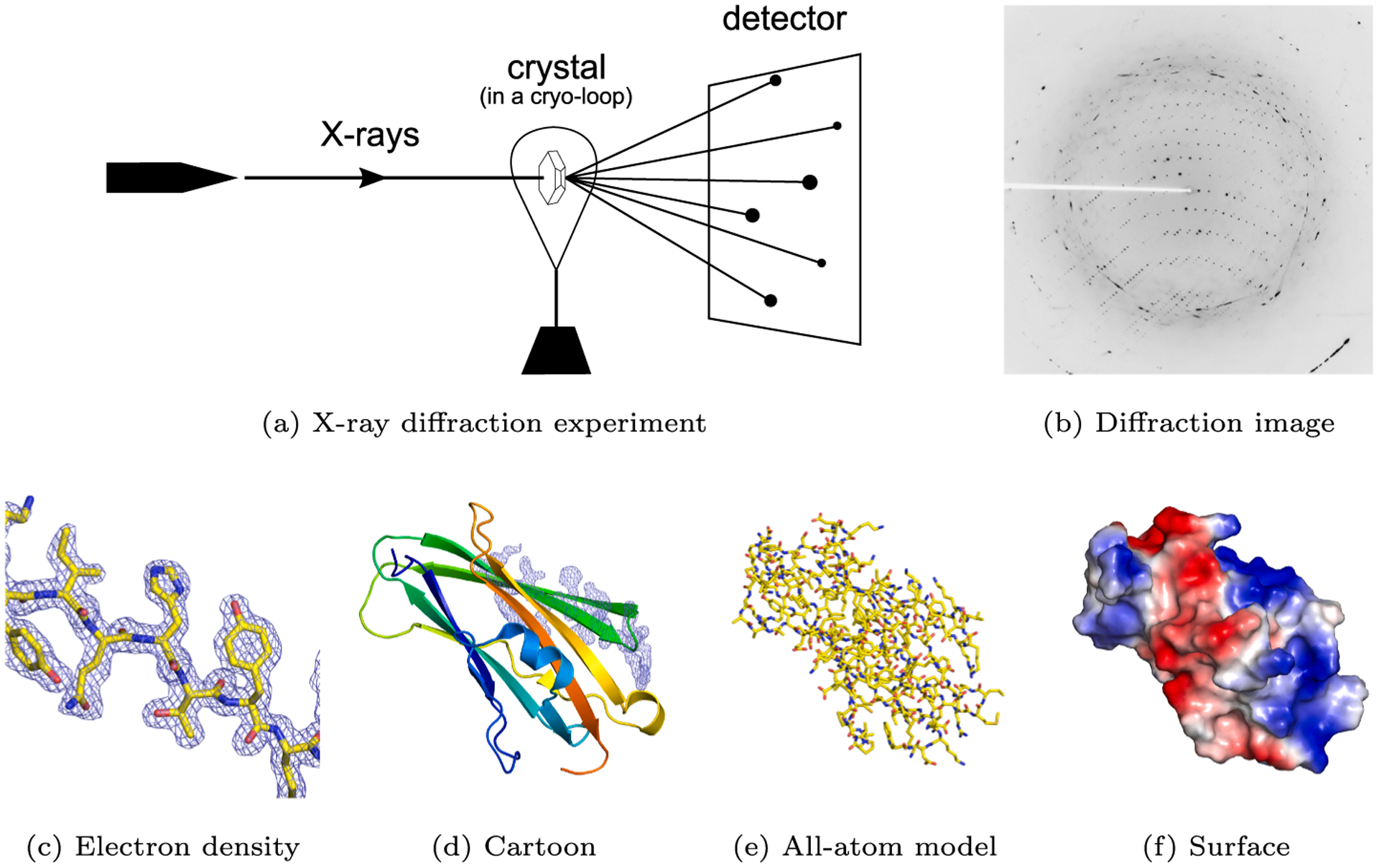
The principle of crystallography (Mayer, 2017). (a) An X-ray beam hits a crystal. (b) The observed diffraction spots (X-ray diffraction image) are the result of the interaction of diffracted photons with the active area of the detector. (c) A fragment of electron density with the associated molecular model of a RhoGDI-mutant protein (PDB code: 2JHU Cooper et al., 2007). (d) A cartoon representation of the entire protein, with the same electron density fragment as on the left. (e) An all-atom representation colored by atom type. (f) A surface representation colored by electrostatic potential.

The quality of an electron density map and, thus, the final structural model depend on the quality of the diffraction image obtained in the X-ray experiment. A number of factors, including an imperfect long-distance order in the crystal, improper cryo-protection, or inaccurate experiment calibration, may strongly affect the diffraction image. Currently, modern experimental synchrotron stations are capable of rapidly collecting thousands of images per crystal (McCarthy et al., 2018) from hundreds of crystals, which are then automatically processed and analyzed (Collins et al., 2018; Pearce et al., 2017; Grabowski et al., 2019). Moreover, millions of images are collected per single X-ray Free Electron Laser experiment (Spence, 2017; Johansson, Stauch, Ishchenko, & Cherezov, 2017; Caleman et al., 2015).

At many synchrotron stations, the raw diffraction images are only scrutinized if the researchers detect processing problems, and the need to efficiently utilize the allocated access time means that an extensive manual evaluation of the images is impractical. Even with more traditional low-throughput experiments, researchers do not always have the time and expertise to thoroughly analyze experiment results in search of flaws in diffraction images. Nevertheless, flaws in diffraction patterns such as loop scattering, strong background radiation, ice rings, diffuse scattering, or other artifacts are fairly common problems in macromolecular crystallography, where the signal to noise ratio is typically weak. When left unhandled, such anomalies can often deteriorate the quality of electron density maps and lead to model misinterpretation (Wlodawer et al., 2018; Raczynska, Shabalin, Minor, Wlodawer, & Jaskolski, 2018). Although several tools for quality assessment have appeared in recent years, most of them focus on electron density maps and structural models (Willard et al., 2003; Urzhumtseva, Afonine, Adams, & Urzhumtsev, 2009; Kowiel et al., 2018; Porebski, Sroka, Zheng, Cooper, & Minor, 2018), whereas those that analyze diffraction images only detect ice rings (Thorn et al., 2017).

In this paper, we propose RefleX—a system for automatic anomaly detection in X-ray diffraction images. RefleX preprocesses raw diffraction data, transforms them into images in Cartesian and polar coordinates, and uses convolutional neural networks to identify seven types of flaws: ice rings, diffuse scattering, background rings, non-uniform detector responses, loop scattering, strong background, and digital artifacts. Since several anomalies can co-occur in one image, the system tackles the problem of multi-label classification.

The main contribution of this paper is the development of an end-to-end anomaly detection system for X-ray diffraction images, which includes a novel beam center detection algorithm. Moreover, the study compares three alternative image representation approaches. Finally, we put forward an open multi-label classification dataset prepared based on 6,311 diffraction images from the Integrated Resource for Reproducibility in Macromolecular Crystallography (Grabowski et al., 2016). To the best of our knowledge, this is the first study using machine learning to classify X-ray diffraction images.

The remainder of the paper is organized as follows. Section 2 provides an overview of the proposed system, discusses each of the analyzed anomalies in detail, presents a novel beam center detection algorithm, and comments on the image representation and classification techniques that were studied. In Section 3, we discuss the experimental results of using the proposed classification pipeline on 6311 diffraction images. Finally, Section 4 concludes the paper and draws lines of future research.

2. Materials and methods

2.1. System overview

Fig. 2 provides an overview of the proposed anomaly detection system. First, raw diffraction data are preprocessed to create normalized (similar for various detector models) images, suitable for visual inspection and image recognition. Next, the system determines the beam center position, i.e., the point on the diffraction image at which the incoming X-ray beam would hit the detector. Using the estimated X-ray beam center, the system converts the image into three alternative data representations: statistical features of rings around the beams center, the image in Cartesian coordinates, and the image in polar coordinates. Finally, the system uses the preprocessed data to train a convolutional neural network.

Fig. 2.

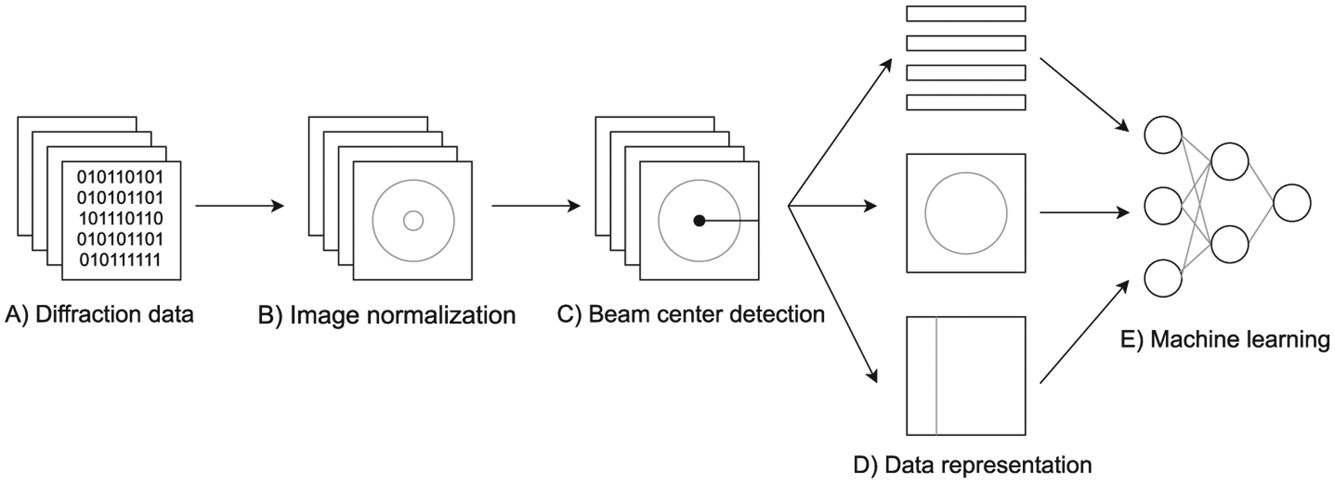
Machine learning pipeline of the proposed anomaly detection system for X-ray diffraction images.

The following sections discuss the main elements of the presented expert system, starting with a description of types of detected anomalies and continuing with the proposed preprocessing algorithms, data representations, and CNN architecture.

2.2. Anomalies

Apart from intensity peaks, X-ray diffraction images can exhibit several visual characteristics. Some of them are the result of clearly aberrant data collection (e.g. digital artifacts), whereas others arise from the nature of the crystalline sample (e.g. diffuse scattering). Most of these characteristics are detrimental to the data collection process, but some may be useful in certain domains. For example, diffuse scattering can be potentially leveraged to model protein motions. Nevertheless, in this study we use the term anomaly to denote all diffraction image characteristics other than clear intensity peaks. Using this definition, the presented study analyzes seven types of anomalies found in X-ray diffraction images:

1. water scattering (Background Ring),

2. diffuse scattering (Diffuse Scattering),

3. ice rings (Ice Ring),

4. loop scattering (Loop Scattering),

5. non-uniform detector responses (Non-uniform Detector),

6. low crystal signal-to-noise ratio (Strong Background),

7. digital artifacts (Artifact).

Fig. 3 shows X-ray diffraction images containing examples of the listed anomalies and Table 1 describes the visual properties, genesis, and possible remedies for each anomaly.

Fig. 3.

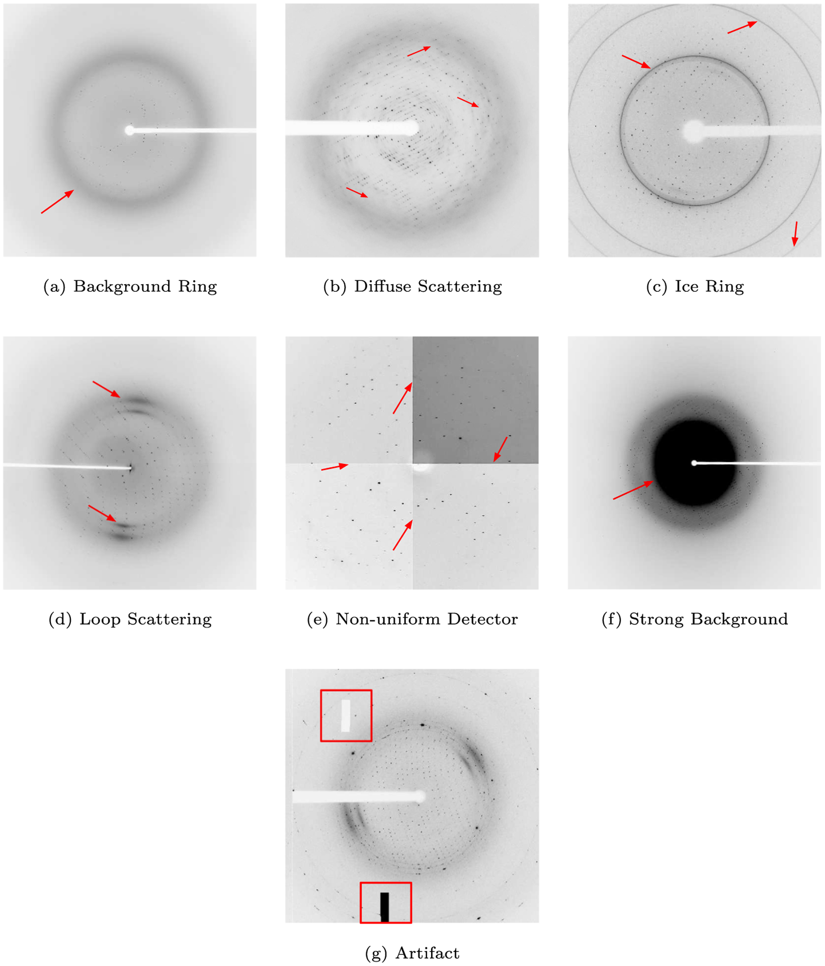
X-ray diffraction images containing the studied anomalies. Images taken from https://proteindiffraction.org (Grabowski et al., 2016).

Table 1.

Summary of the studied X-ray diffraction anomalies.

Anomaly	Visual description	Genesis	Possible actions
Background Ring	Blurry circular shadow centered around the primary beam position.	Scattering caused by partial ordering of the solvent molecules, or amorphous ice.	Diffraction images can be optimized to deal with this issue.
Diffuse Scattering	Blurry, gray smudges.	Caused by parts of the crystal not being well ordered.	Early detection allows for automated screening of different crystallization conditions.
Ice Ring	Thin, well-defined, concentric rings of varying strength.	Result when the crystal is not properly cryo-protected, stored, or shipped.	Indicates problems with vitrification. Early detection can be used for screening flash cooling conditions or automating annealing protocols.
Loop Scattering	Two or four small, arched shadows, located on opposite sides of the beam position.	Scattering caused by materials used to hold the crystal (loop).	In some cases, the quality of the data can be improved by increasing data redundancy.
Non-uniform Detector	Visible differences between the darkness of panels.	Inconsistent detectors making up the detector array cause uneven background shade.	Early detection of substantial non-uniformity allows for troubleshooting and proper planning before data collection.
Strong Background	Dark, full circle covering the center of the image.	The crystal’s suspension liquid absorbs and uniformly scatters X-rays.	Early detection allows for the modification of the data collection strategy, to compensate for the high background.
Artifact	Missing random (blocks) of pixels; black or white solid areas.	Data corruption, electronics failure, read/compression error.	Detection allows for early troubleshooting, detector repairs, and data collection planning.

Some of the anomalies (artifacts, diffuse scattering, non-uniform detectors) are very subtle and can be difficult to spot at first glance, whereas other problems (strong background, ice rings, loop scattering) are fairly easy to notice. Nevertheless, the anomalies may or may not appear on all the gathered X-ray images, meaning that one would have to analyze all (usually between 180 and 9,000) experimental images to be sure whether or not a given anomaly occurred. Therefore, automatic detection of the above-mentioned anomalies is of high practical value compared to manual visual inspection.

2.3. Data selection and preprocessing

To create and evaluate the proposed image classification system, 6,311 diffraction images were taken from the Integrated Resource for Reproducibility in Macromolecular Crystallography (https://proteindiffraction.org) (Grabowski et al., 2016). The first image from every X-ray diffraction dataset stored at proteindiffraction.org (as of March 23, 2018) was selected, thereby representing 6,311 different experimental conditions.

Since the X-ray diffraction images were taken at several synchrotrons which use a variety of detectors, the images were first converted from their proprietary data formats into 2D (numpy Oliphant, 2006) arrays of floats. Next, the numpy arrays were cleaned, by removing NaN (Not a Number) values that can appear in readings from some machines on the boundaries between detector panels. These readings are the effect of slight gaps between these panels, and form a grid, as presented in Fig. 4. Finally, to standardize images recorded by detectors of different sensitivity, the values in the numpy arrays were clipped to values no higher than the 95th percentile of a given image and then normalized so that all values are represented as integers and fall into the 0–255 range. With the grid removed and intensities normalized, the resulting arrays were saved as 512 × 512 PNG files. This size has been selected empirically, as it allows the classifier to train fairly quickly, while obtaining relatively good classification results. Resizing was done using the Nearest Neighbor Interpolation method (Bradski, 2000), which preserves the original pixel values from the input image and is computationally efficient. We chose nearest neighbor interpolation because it does not introduce anti-aliasing and, therefore, does not blur X-ray intensity peaks.

Fig. 4.

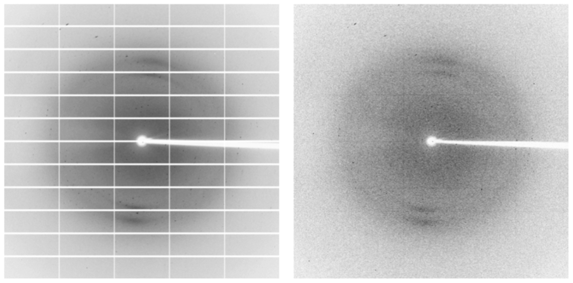
Diffraction image before (left) and after (right) removing the detector-gap grid.

The resulting 6,311 normalized images were manually labeled according to the seven anomaly types described in Section 2.2. A given X-ray diffraction image can contain no anomalies, a single anomaly, or multiple anomalies, with classes distributed as shown in Fig. 5a. Interestingly, according to the bias-corrected V-Cramer measure (Bergsma, 2013; Cramér, 1946), there is no strong correlation between any pair of classes (Fig. 5b); therefore, we used standard random stratified sampling to split the data into training, validation, and test sets, while preserving label proportions within each set.

Fig. 5.

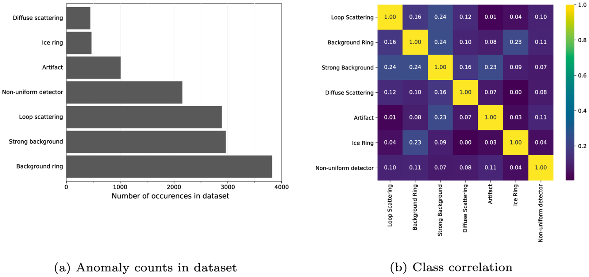
Training data characteristics: (a) class counts; (b) pairwise class correlation according to bias-corrected Cramer’s V measure.

The final dataset containing normalized X-ray diffraction images, including stratified division into training, validation, and testing data has been made publicly available through Zenodo: https://zenodo.org/record/2605120/ (Czyzewski, Krawiec, Brzezinski, & Porebski, 2019).

2.4. Beam center detection algorithm

X-ray diffraction images often come with metadata, which specify the primary beam position, among other things. However, this information is not always available or is inaccurate. This lack of reliable information served as the motivation for the development of a center-detection algorithm. In our system, the beam position is required for the generation of alternative image representations (discussed in the following section), but the method presented below could also be very useful for X-ray data processing packages (Winn et al., 2011; Adams et al., 2010; Minor, Cymborowski, Otwinowski, & Chruszcz, 2006). The pseudo-code of our method is presented in Algorithm 1.

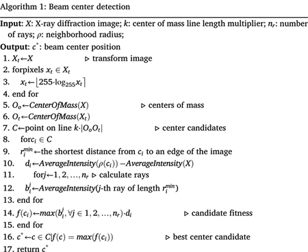
As the input of our method, we take a grayscale image X (each pixel’s value is an integer in the 0–255 range). We create a new, corresponding image X_t by applying the following function to every pixel of the original image: t(x) = ⌊255·log₂₅₅x⌋ (where the brackets symbolize rounding to the nearest integer). This normalizes the input image so that outliers become less prominent.

We use image moments (Bradski, 2000) to calculate the center of mass of the original image (O_o) and the center of mass of the transformed image (O_t). We mark the coordinates of these two points on the original image and draw a line of length k·|O_oO_t| that passes through O_o and O_t, and whose center is at O_o, where k is a user-defined parameter. In the final system implementation we used k = 4. We use Bresenham’s algorithm (Bresenham, 1965) to obtain a raster representation of the line traversing O_o and O_t. All points on this line form a set of center candidates C and will be individually evaluated in the next stage. Fig. 6 visualizes the mentioned steps.

Fig. 6.

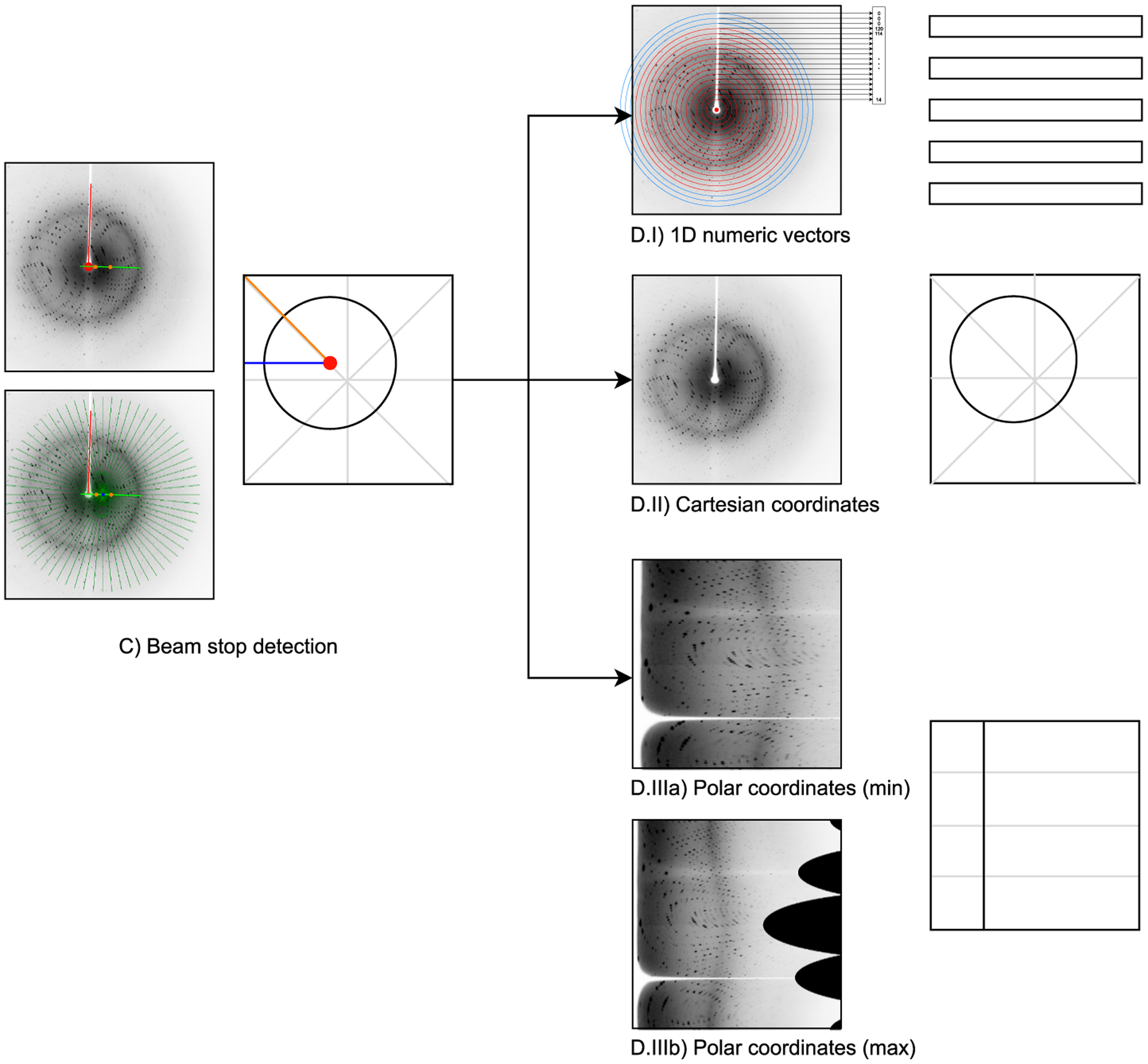
Detailed schematic of steps C and D of the system’s processing pipeline (Fig. 2). (C): Example visualization of the beam center detection procedure. Left top: The set C of center candidates is outlined as the green line, the centers of mass (O_o and O_t) are shown with orange points, and the red point marks the detected center c*. Left bottom: Rays depicted as green lines centered in an example beam center candidate c_i (blue point) with the beam stop shadow highlighted with a red line. Right: schematic of the results of beam center detection; red point marks the detected center, blue and orange lines are the min and max radii used for polar coordinate interpolations. (D): Alternative image representations.

In the second stage of the algorithm, we attempt to find the beam stop shadow (white strip labeled with a red line in Fig. 6). For this purpose, we iterate through C, and for each center candidate c_i we generate n_r = 256 rays. Each ray originates at c_i and is of length $r_i^{min}$, where $r_i^{min}$ is defined as the shortest distance from c_i to an edge of the image. The n_r rays are spaced evenly, α = 360°/n_r apart from each other. For each ray, we compute its average pixel value $b_i^j$ (brightness). We also calculate the difference d_i between the average pixel value in the neighborhood of radius ρ of c_i and the average pixel value of the entire image. In our experiments we used ρ = 1.

Finally, for each candidate center c_i, we compute the fitness of c_i as $f(c_i)=max(b_i^j,\forall j\in 1,2,\dots ,n_r)\cdot d_i$. Using f(c_i), the detected center c* is chosen as the center candidate whose computed fitness f was largest: c* = c ∈ C|f(c) = max(f(c_i)).

The proposed algorithm is inspired by the fact that most X-ray diffraction images have a white strip (beam stop shadow), one end of which covers the primary beam position we want to find. The endpoint of this strip is often surrounded by a white area—the beam stop protecting the detector from direct beam exposition. The fitness function f(·) aims to promote those center candidates which might be in this strip endpoint area. Some X-ray diffraction images, unfortunately, do not have a visible white strip or white center (e.g. the beam stop mount is transparent). The proposed algorithm is not specifically designed to deal with such cases; however, in the absence of a strip, the centers of mass O_o and O_t are usually so close to each other that the set C of candidates is relatively small and contains points close to the actual center.

2.5. X-ray diffraction image representations

As input to the classification algorithms, we considered three alternative image representations:

1. Numeric feature vectors,

2. Cartesian coordinates,

3. Polar coordinates.

In the numeric vector representation, we decided to use a standard, general-purpose machine learning strategy and perform manual feature engineering. Since X-ray diffraction patterns are usually circular in nature, the engineered features concentrated on compressing a 2-D diffraction image to a 1-D vector. This was done by calculating a selected statistic (e.g. median) of all pixels laying at a given distance (layer) from the beam center position (Fig. 6 D.I). Because the diffraction images are a discrete matrix of points, determining which points belong to each layer is a non-trivial task. We used a variation of the Midpoint Circle Algorithm (Bresenham, 1977) to find sets of points such that the circles they form are non-overlapping and leave no gaps in between consecutive layers. If a circle did not entirely fit in the image (Fig. 6 D.I blues circles), we used only those pixels which are within the boundaries of the image to calculate a given statistic. Moreover, from each layer, we also excluded those points that belong to the beam stop shadow (white strip), if one is present. This was done by excluding those lines originating from the beam stop position that were at least 4·σ from the mean pixel intensity of all lines originating from the image center (Fig. 6 C). The final feature vectors consisted of 240 numeric values, as this is slightly less than half of the side of an image (which would be 512/2 = 256px). For most diffraction images this means that even the last layer formed from the largest circle will entirely fit inside the image, omitting the corners of the image, which rarely contain any meaningful artifacts. The set of 1D vectors computed using this method included the following statistics: minimum, maximum, mean, median, variance, 5th percentile, 95th percentile.

The Cartesian coordinates representation did not require any preprocessing and consisted of the normalized X-ray diffraction image. Such a representation deemed suitable for convolutional neural networks, which extract features during their learning process.

Finally, the polar coordinates representation attempted to ‘unwrap’ the generally circular X-ray diffraction pattern. For this purpose, we used the LinearPolar method from the OpenCV library (Bradski, 2000), specifying the beam center position as the center of the image. We tried using two different interpolation methods: min and max. The min interpolation method transforms an area bounded by a circle with a center in the beam center position and a radius defined by the distance from the detected image center to the closest image border (Fig. 6 C blue line). This means that a significant portion of the original image (namely the peripheral area) is no longer represented after the polar transformation. This method does, however, have the upside of not containing synthetically produced interpolation artifacts. The max interpolation uses a radius defined by the distance from the detected image center to the closest image corner (Fig. 6 C orange line). This means that much more of the information from the original image is retained after the polar transformation, however, a significant part of the transformed area is outside the bounds of the original image. This data needs to be somehow filled in, and the LinearPolar function does this by interpolating values from a point’s neighborhood (when a point is sufficiently close to points that contain valid data) or assigning the value 0 (when the points entire neighborhood is also invalid). Fig. 6 presents the difference in the effects of the polar transformation when the min and max interpolation parameters are used.

2.6. Classification

For the last step of the proposed anomaly detection system, we tested different classification algorithms with different image representations.

The numeric vector representation served as input for four general-purpose classifiers implemented in the scikit-learn (Pedregosa et al., 2011) library: Support Vector Machines (SVM), Naive Bayes (NB), k-Nearest Neighbors (KNN), and Random Forest (RF). The general-purpose classifiers were chosen for their versatility: SVM was selected as a representative of linear classifiers, NB as a representative of probabilistic classifiers, KNN as a distance-based classifier, and RF as a tree-based learner. The general-purpose classification algorithms were trained using the One-vs-All (OvA) strategy (Bishop, 2007), i.e., each classifier was trained to predict one class of anomaly at a time. Therefore, effectively seven classification models had to be trained per algorithm, giving 4 × 7 = 28 models in total.

To find the best parameters for the general-purpose classifiers (SVM, NB, KNN, RF), we used the GridSearchCV method of scikit-learn and specified the indices of training and validation examples (test examples were held out from this procedure). In SVM, we used L2-regularization and optimized the regularization penalty C ∈ {1, 5, 10}. In NB, we tuned the smoothing ∈ {1e −5, 1e −7, 1e −9, 1e −10} parameter, which determines the largest variance of all features that is added to variances for calculation stability of the Gaussian approximation of numeric features. In KNN, we tuned the number of nearest neighbors k ∈{5,7,10,15,20,30,50}. Finally, in RF we tuned the number of trees in the forest trees ∈ {10,20,50,100,200}. The remaining parameters were left with default scikit-learn values.

The remaining image representations (Cartesian, Polar min, Polar max) were fed into fast.ai implementations of resnet Convolutional Neural Networks (CNNs) pretrained on imagenet competition data (He, Zhang, Ren, & Sun, 2016). Contrary to general-purpose algorithms, CNNs were trained for the multi-label classification of all seven classes of anomaly simultaneously.

We developed our own implementation of grid search to adjust the hyper-parameters of the convolutional neural networks we created using the fast.ai library. This method was written as an independent Python script and is available on the project’s GitHub (https://github.com/aczyzewski/refleX).

We tested each combination of the following hyper-parameters:

• image size (scaling) ∈ {64, 128, 256, 512},

• batch size ∈ {8, 16, 32, 64};

• (pretrained) network architecture ∈ {ResNet-18, ResNet-34, ResNet-50}.

We additionally set the following hyper-parameters, which stayed constant throughout the entire training process:

• dropout rate = 0.5;

• early stopping = 12 epochs;

• image augmentation method: RandomLighting + RandomDihedral for Cartesian representation; RandomLighting for polar representation; where RandomLighting increases or decreases an image’s pixel brightness and contrast by random values between −10% and +10%, and RandomDihedral rotates an image by random multiples of 90 degrees and/or reflections.

Another hyper-parameter that had to be tuned when training neural networks is the learning rate. This parameter, however, was set using a series of selected heuristics that speed up network training (Howard & Ruder, 2018; Smith & Topin, 2017; Smith, 2015). The heuristics used to dynamically estimate the learning rate, as well as other methods used to enhance the predictive performance of the final model are described below.

2.6.1. Pretrained network

We used a pretrained network architecture and adapted it to our training images. This way the network did not have to learn image recognition from scratch, rather adapt itself to new images. We used resnet architectures with 16, 34, and 50 layers, pretrained on imagenet competition data (He et al., 2016).

2.6.2. Image rescaling

The model was first trained on images rescaled to a small size, and then consecutively on larger and larger images until reaching the original size (Howard & Ruder, 2018). Our model was being trained on the following sizes of the same image: 64 × 64, 128 × 128, 256 × 256, 512 × 512.

2.6.3. Freezing layers

We divided the training process into two stages. In the first stage, only the last (fully-connected) layers of the model are being trained, and the rest of the weights (convolutional layers) are “frozen”. Once the training is done in the first stage, the second stage can be started where all model weights are “unfrozen” and can be updated during training (Howard & Ruder, 2018).

2.6.4. Local learning rates

This technique assumes a lower learning rate for the early layers of the network, because they isolate the most basic features that do not require full training. In our case, we divided the layers into four sets, where the last group (containing the fully connected layers) contains the learning rate parameter determined in the beginning, and each “earlier” set of layers has a parameter twice smaller in respect to the next set. Cosine annealing with restarts This heuristic involved cyclically changing the learning rate, increasing the number of epochs, and restarting the learning process. The training process was divided into cycles. In each cycle, the learning rate parameter is slowly decreased (linearly or based on the cosine function) along with subsequent epochs, until the final iteration is reached, in which it returns to its initial value (restart) (Smith, 2015). Restarts allow the optimizer to escape local minima. Prolonging the cycle means that each cycle, until it achieves the minimum learning rate, needs n times more epochs than the previous one. In our implementation n = 2. The initial learning rate was established using the super-convergence paradigm proposed in Smith and Topin (2017).

The best parameters for each of the three CNNs are presented in Table 2.

Table 2.

Best hyper-parameters for CNN classifiers.

	CNN: Cartesian	CNN: Polar-min	CNN: Polar-max
Architecture	ResNet-34	ResNet-34	ResNet-34
Parameters	21.3 M	21.3 M	21.3 M
Dropout	0.5	0.5	0.5
Image size	64 – > 512	64 – > 512	64 – > 512
Batch size	16	8	8
Validation loss	0.15024	0.1616	0.1639
Early stopping after	12 epochs	12 epochs	12 epochs
Learning rate (last layers)	0.008272	0.008642	0.006792
Learning rates (all layers)	[0.001034, 0.002068, 0.004136, 0.008272]	[0.00108, 0.00216, 0.004321, 0.008642]	[0.000849, 0.001698, 0.003396, 0.006792]
Epochs	700	550	650

3. Results and discussion

3.1. Center detection algorithm

Out of 6,311 diffraction images analyzed in this study, 2,090 contained verified information about exact beam center positions and were used for testing the proposed center detection algorithm. Fig. 7 presents a heatmap of beam center positions found in these images. It can be noticed that the vast majority of beam center positions were at the center of the detector panel or in its near vicinity. Therefore, a naive approach to predicting the beam center position would be to return the image’s center. We used such a naive approach as a baseline to compare our algorithm against.

Fig. 7.

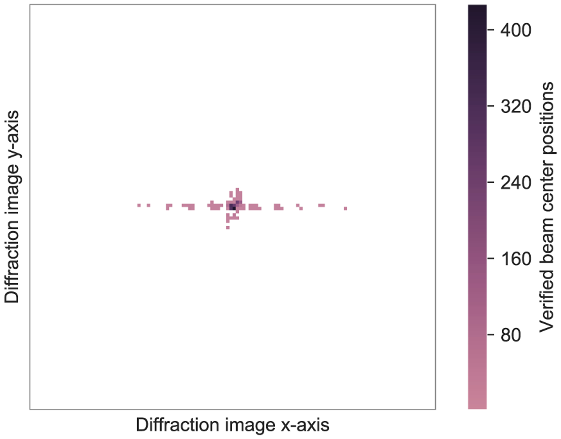
Heatmap of beam center positions. Each point on the heatmap corresponds to a 8 × 8-pixel square on a diffraction image.

Given the true and predicted beam center position, the prediction error was calculated as the Euclidean distance between the two. To make the errors comparable, all diffraction images were re-scaled to 1024 × 1024 (the size of the smallest raw diffraction image). Individual errors were aggregated by calculating the Mean Absolute Error (MAE) and the Root Mean Square Error (RMSE).

The proposed algorithm achieved a MAE of 7.67 pixels compared to 12.73 obtained by the naive approach. Similarly, the proposed algorithm achieved a RMSE of 11.87 clearly outperforming the naive approach which obtained a RMSE of 27.93. Seeing that 7.67/11.87 pixels correspond to 0.75/1.16% of each side of a test image, the attained average center detection performance can be considered sufficient for transforming images to polar coordinates.

3.2. Classifier comparison

The analyzed dataset of 6,311 labeled diffraction images was divided into three subsets using random stratified sampling: a training set (5048 images), validation set (631 images), and testing set (632 images). The proposed system was tested using seven classifier-representation pairs: Support Vector Machines (SVM), Naive Bayes (NB), k-Nearest Neighbors (KNN) and Random Forest (RF) used vector representations, whereas convolutional neural networks used the Cartesian (CNN: Cartesian), and polar coordinates (CNN: Polar-min, CNN: Polar-max) representations. Hyper-parameters of each of the above classifiers were optimized using the validation set. Reproducible experiment scripts are available on GitHub at: https://github.com/aczyzewski/refleX.

The final evaluation was done on tuned classifiers using the test set by calculating aggregated (multi-label) and class-specific evaluation measures. Aggregated measures assessed classification performance for all seven classes simultaneously, and included macro-averaged (^M) aggregates of Precision (Prec.^M), Recall (Rec.^M), F1-score (F1^M), F2-score (F2^M), Matthews Correlation Coefficient (MCC^M) (Japkowicz & Shah, 2011), as well as standard multi-label classification measures, i.e. Jaccard Index (JI) and Exact Match Ratio (EMR) (Read & Hollmén, 2014). Class-specific measures evaluated classifier performance for each anomaly separately on a one-vs-all basis using: Accuracy (Acc.), Precision (Prec.), Recall (Rec.), F1-score (F1), and the area under the ROC curve (AUC).

Table 3 presents classifier performance according to multi-label measures, whereas Tables 4,5 and Fig. 8 show anomaly-specific results.

Table 3.

Multi-label classification performance of four general-purpose classifiers and three convolutional neural networks. Performance measured using macro-averaged precision (Prec.^M), macro-averaged recall (Rec.^M), macro-averaged F1-score (F1^M) and F2-score (F2^M), macro-averaged Mathew’s Correlation Coefficient (MCC^M), Jaccard Index (JI), and exact match ratio (EMR). Best values for each measure highlighted in bold.

Classifier	Prec.M	Rec.M	F1M	F2M	MCCM	JI	EMR
SVM	0.59	0.66	0.52	0.63	0.36	0.41	0.02
NB	0.48	0.69	0.53	0.64	0.31	0.43	0.05
KNN	0.76	0.52	0.55	0.67	0.44	0.60	0.31
RF	0.83	0.60	0.66	0.76	0.60	0.71	0.45
CNN: Cartesian	0.88	0.86	0.87	0.87	0.81	0.83	0.65
CNN: Polar-min	0.88	0.84	0.85	0.86	0.80	0.83	0.63
CNN: Polar-max	0.89	0.84	0.86	0.86	0.81	0.83	0.65

Table 4.

Table of class-specific predictive performance of each of the tested general-purpose classifiers. Performance is measured using accuracy (Acc.), precision (Prec.), recall (Rec.), F1-score (F1), and the area under the ROC curve (AUC).

Classifier	Class	Acc.	Prec.	Rec.	F1	AUC
SVM	Artifact	0.85	0.81	0.31	0.45	0.65
	Background Ring	0.72	0.73	0.85	0.79	0.68
	Diffuse Scattering	0.93	0.44	0.25	0.32	0.61
	Ice Ring	0.14	0.08	0.98	0.14	0.52
	Loop Scattering	0.70	0.79	0.40	0.53	0.66
	Non-unif. Detector	0.45	0.39	0.96	0.55	0.56
	Strong Background	0.90	0.89	0.90	0.90	0.90
NB	Artifact	0.78	0.46	0.62	0.53	0.72
	Background Ring	0.61	0.66	0.74	0.70	0.57
	Diffuse Scattering	0.45	0.10	0.84	0.17	0.63
	Ice Ring	0.80	0.17	0.46	0.25	0.64
	Loop Scattering	0.62	0.53	0.71	0.61	0.63
	Non-unif. Detector	0.68	0.55	0.63	0.59	0.67
	Strong Background	0.87	0.90	0.83	0.86	0.87
KNN	Artifact	0.87	0.80	0.48	0.60	0.72
	Background Ring	0.72	0.79	0.74	0.76	0.71
	Diffuse Scattering	0.93	0.60	0.07	0.12	0.53
	Ice Ring	0.93	1.00	0.09	0.16	0.54
	Loop Scattering	0.71	0.62	0.79	0.69	0.72
	Non-unif. Detector	0.75	0.69	0.53	0.60	0.70
	Strong Background	0.89	0.85	0.93	0.89	0.89
RF	Artifact	0.91	0.91	0.60	0.72	0.79
	Background Ring	0.86	0.87	0.91	0.89	0.84
	Diffuse Scattering	0.93	0.50	0.05	0.08	0.52
	Ice Ring	0.95	1.00	0.33	0.49	0.66
	Loop Scattering	0.83	0.82	0.76	0.79	0.82
	Non-unif. Detector	0.81	0.80	0.63	0.71	0.77
	Strong Background	0.93	0.92	0.94	0.93	0.93

Table 5.

Table of class-specific predictive performance of each of the tested CNNs. Performance is measured using accuracy (Acc.), precision (Prec.), recall (Rec.), F1-score (F1), and the area under the ROC curve (AUC).

Classifier	Class	Acc.	Prec.	Rec.	F1	AUC
CNN: Cartesian	Artifact	0.94	0.91	0.79	0.85	0.89
	Background Ring	0.92	0.95	0.93	0.94	0.92
	Diffuse Scattering	0.96	0.74	0.59	0.66	0.79
	Ice Ring	0.99	0.92	0.98	0.95	0.99
	Loop Scattering	0.94	0.90	0.97	0.93	0.95
	Non-unif. Detector	0.87	0.83	0.78	0.80	0.85
	Strong Background	0.94	0.91	0.97	0.94	0.94
CNN: Polar-min	Artifact	0.93	0.88	0.77	0.82	0.87
	Background Ring	0.91	0.94	0.92	0.93	0.91
	Diffuse Scattering	0.95	0.71	0.50	0.59	0.74
	Ice Ring	0.99	0.93	0.93	0.93	0.96
	Loop Scattering	0.95	0.92	0.96	0.94	0.95
	Non-unif. Detector	0.89	0.84	0.84	0.84	0.88
	Strong Background	0.91	0.90	0.93	0.91	0.92
CNN: Polar-max	Artifact	0.92	0.90	0.70	0.79	0.84
	Background Ring	0.90	0.93	0.90	0.92	0.90
	Diffuse Scattering	0.97	0.85	0.64	0.73	0.81
	Ice Ring	0.98	0.87	0.89	0.88	0.94
	Loop Scattering	0.96	0.94	0.96	0.95	0.96
	Non-unif. Detector	0.89	0.84	0.84	0.84	0.88
	Strong Background	0.93	0.92	0.94	0.93	0.93

Fig. 8.

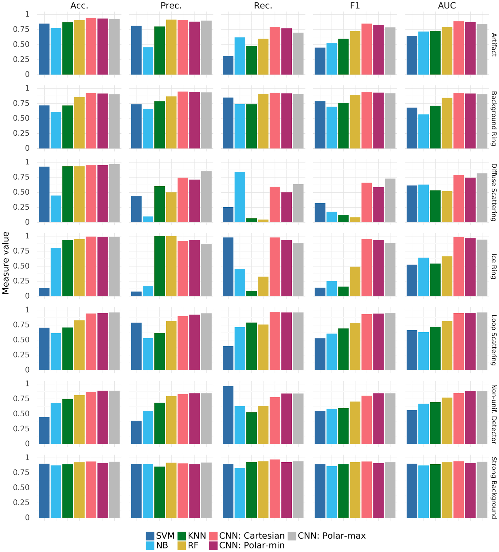
Bar plot presenting the class-specific performance (columns) of each of the seven analyzed classifiers on each of the anomaly classes (rows). Performance is measured using accuracy (Acc.), precision (Prec.), recall (Rec.), F1-score (F1), and the area under the ROC curve (AUC). The numeric data used to generate this plot are presented in Tables 4 and 5.

Table 3 clearly shows that CNN: Cartesian is consistently better than any other of the tested classifiers on all performance measures with the small exception of macro-averaged precision, which is 0.01 better for CNN: Polar-max. It is worth noting, that the differences between CNNs are generally around 0.01–0.02, whereas general-purpose classifiers have significantly lower predictive performance than CNNs.

The above observations are confirmed when looking at anomaly-specific performance presented in Tables 4,5 and Fig. 8. One can notice that the biggest differences between general-purpose classifiers and CNNs are most visible on anomalies that are the least frequent and affect small parts of the diffraction images: Diffuse Scattering and Ice Ring. Anomaly-specific results also reveal that CNN: Polar-max is slightly better than CNN: Cartesian at detecting Diffuse Scattering, Loop Scattering and Non-uniform Detectors. This suggests that, in the future, better performance could possibly be obtained by, for example, combining different image representations.

Since general-purpose algorithms and CNNs were trained using different libraries (scikitlearn, fast.ai) on different architectures (CPU, GPU), there is no objective way of comparing training time. However, regardless of the exact measure used to estimate the broadly understood ‘computational cost’ of these training schemes, it is evident that the chosen general-purpose classifiers can be trained orders of magnitude quicker than CNNs. In our experiments the general-purpose models trained for no more than 10 min each, while each CNN took several hours.

3.3. Discussion

The vector representation used by general-purpose classifiers does not convey as much information as the image representations used by CNNs. On the other hand, the impact of representation choice on CNN performance is relatively small—the three models (CNN: Cartesian, CNN: Polar-min, CNN: Polar-max) are within 0.05 of one another on all performance measures and every type of anomaly. Interestingly, the Cartesian representation performs better than Polar-min and Polar-max on two of the ‘circular’ anomalies: background rings and ice rings. This might be the result of slight inaccuracies in the detection of the image center or the fact that the transformation to polar coordinates strongly alters image corners, which sometimes are the only area with visible rings. However, polar representations are better than Cartesian in detecting non-uniform detectors and, in case of Polar-max, diffuse scattering. This performance advantage may be the result of scattering intensity differences in a circular way, creating visual artifacts that more closely correspond to pre-existing convolutional features found in the ImageNet-pretrained network. This finding relates to the problem of domain similarity in transfer learning (Bernico, Li, & Zhang, 2019; Zhong et al., 2018), and suggests that abstract experimental images can be potentially preprocessed to resemble ImageNet features prior to training.

The results show that convolutional neural networks can be successfully used to detect anomalies in X-ray diffraction images. Being a premier on using machine learning to analyze raw diffraction data, this study shows that current pattern recognition algorithms can prove useful in analyzing images which are rarely examined by humans. Importantly, this particular study deals with structural biology data, which provides the structural basis for our understanding of life and plays a crucial role at the interface of physics, chemistry, and biology (Baker, 2018; Blundell, 2017; Pomés et al., 2015). Seeing that more and more elements of drug screening pipelines and other protein analyses are attempted to be done without human supervision (Blundell, Jhoti, & Abell, 2002; Bowler, Svensson, & Nurizzo, 2016), this work may be useful in automating crucial scientific processes even further.

4. Conclusions and future work

In this paper, we have put forward an expert system for the automatic detection of anomalies in X-ray diffraction images. To this end, we have described seven types of anomalies, collected 6,311 diffraction images, and labeled them according to the proposed anomaly definitions. The labeled images served as the basis for an extensive comparative analysis of the performance of seven different classifiers using three alternative image representations. The best classifier achieved an overall Jaccard Index of 0.83, with 0.87 classification accuracy on the most difficult anomaly class. The remaining six classes were classified with an accuracy of over 0.92. These values are satisfactory and indicate that the chosen model can be feasibly used for automatic anomaly detection at X-ray beamlines. This study lays a groundwork for on-the-fly analysis of X-ray diffraction images in high-throughput settings that can be used for online decision making and developing data collection strategies that maximize data quality without compromising throughput. Careful analysis of artifacts presented in this paper may also influence the development of X-ray detectors and help tune-up existing synchrotron facilities.

Future research directions include the development of more problem-specific classification models and data representations. There is still potential for improving the accuracy of the center detection algorithm, and one could design other data features, e.g., by employing Zernike moment invariants (Khotanzad & Hong, 1990). Furthermore, recent developments in image generation techniques (Pathak, Krähenbühl, Donahue, Darrell, & Efros, 2016; Yeh, Chen, Lim, Hasegawa-Johnson, & Do, 2016) could be used to automatically remove anomalies from diffraction images. Training of such a system could rely on injected or simulated anomalies (Holton, Classen, Frankel, & Tainer, 2014) and potentially represent a huge step forward in restoring currently unusable data. Moreover, there are still unexplored research topics concerned with machine learning on diffraction images, such as automatic selection of diffraction image areas affected by an anomaly or feature transferability between real-world and abstract image domains. Our work demonstrates that, with proper preprocessing and tuning, images with abstract features can reuse classifiers trained on images with real objects and achieve good classification accuracy using a limited number of labeled samples. This approach may be considered as a starting point for other raw experimental image assessment systems, e.g. for the automatic analysis of power spectra images in the rapidly growing field of cryogenic electron microscopy (cryo-EM) (Bai, McMullan, & Scheres, 2015; McMullan, Vinothkumar, & Henderson, 2015).

References

- Adams PD, Afonine PV, Bunkóczi G, Chen VB, Davis IW, Echols N, Headd JJ, Hung L-W, Kapral GJ, Grosse-Kunstleve RW, McCoy AJ, Moriarty NW, Oeffner R, Read RJ, Richardson DC, Richardson JS, Terwilliger TC, & Zwart PH (2010). PHENIX: a comprehensive Python-based system for macromolecular structure solution. Acta Crystallographica Section D, 66, 213–221. [DOI] [PMC free article] [PubMed] [Google Scholar]
- Bai X-C, McMullan G, & Scheres SH (2015). How cryo-em is revolutionizing structural biology. Trends in Biochemical Sciences, 40, 49–57. [DOI] [PubMed] [Google Scholar]
- Baker EN (2018). Crystallography and the development of therapeutic medicines. IUCrJ, 5, 118. [DOI] [PMC free article] [PubMed] [Google Scholar]
- Bergsma W (2013). A bias-correction for Cramér’s V and Tschuprow’s T. Journal of the Korean Statistical Society, 42. [Google Scholar]
- Bernico M, Li Y, & Zhang D (2019). Investigating the impact of data volume and domain similarity on transfer learning applications. In Arai K, Bhatia R, & Kapoor S (Eds.), Proceedings of the Future Technologies Conference (FTC) (pp. 53–62). [Google Scholar]
- Bishop CM (2007). Pattern recognition and machine learning. Information science and statistics (5th ed.). Springer. [Google Scholar]
- Blundell T, & Johnson L (1976). Protein crystallography. Molecular biology. Academic Press. [Google Scholar]
- Blundell TL (2017). Protein crystallography and drug discovery: recollections of knowledge exchange between academia and industry. IUCrJ, 4, 308–321. [DOI] [PMC free article] [PubMed] [Google Scholar]
- Blundell TL, Jhoti H, & Abell C (2002). High-throughput crystallography for lead discovery in drug design. Nature Reviews Drug Discovery, 1, 45. [DOI] [PubMed] [Google Scholar]
- Bowler MW, Svensson O, & Nurizzo D (2016). Fully automatic macromolecular crystallography: The impact of massif-1 on the optimum acquisition and quality of data. Crystallography Reviews, 22, 233–249. [Google Scholar]
- Bradski G (2000). The OpenCV Library. Dr. Dobb’s Journal of Software Tools. [Google Scholar]
- Bresenham J (1977). A linear algorithm for incremental digital display of circular arcs. Communications of the ACM, 20, 100–106. [Google Scholar]
- Bresenham JE (1965). Algorithm for computer control of a digital plotter. IBM Systems Journal, 4, 25–30. [Google Scholar]
- Caleman C, Tîmneanu N, Martin AV, Jönsson HO, Aquila A, Barty A,Scott HA, White TA, & Chapman HN (2015). Ultrafast self-gating bragg diffraction of exploding nanocrystals in an x-ray laser. Optics Express, 23, 1213–1231. [DOI] [PubMed] [Google Scholar]
- Collins PM, Douangamath A, Talon R, Dias A, Brandao-Neto J, Krojer T, & von Delft F (2018). Chapter eleven – Achieving a good crystal system for crystallographic x-ray fragment screening. In Lesburg CA (Ed.), Modern Approaches in Drug Discovery (pp. 251–264). Academic Press; volume 610 of Methods in Enzymology. [DOI] [PubMed] [Google Scholar]
- Cooper DR, Boczek T, Grelewska K, Pinkowska M, Sikorska M, Zawadzki M, & Derewenda Z (2007). Protein crystallization by surface entropy reduction: optimization of the SER strategy. Acta Crystallographica Section D, 63, 636–645. [DOI] [PubMed] [Google Scholar]
- Cramér H (1946). Mathematical methods of statistics (PMS-9) (Vol. 9). Princeton University Press. [Google Scholar]
- Czyzewski A, Krawiec F, Brzezinski D, & Porebski PJ (2019). Reflex: X-ray diffraction images dataset. 10.5281/zenodo.2605120. [DOI] [PMC free article] [PubMed] [Google Scholar]
- Grabowski M, Cymborowski M, Porebski PJ, Osinski T, Shabalin IG, Cooper DR, & Minor W (2019). The integrated resource for reproducibility in macromolecular crystallography: Experiences of the first four years. Structural Dynamics, 6, Article 064301. [DOI] [PMC free article] [PubMed] [Google Scholar]
- Grabowski M, Langner KM, Cymborowski M, Porebski PJ, Sroka P, Zheng H, Cooper DR, Zimmerman MD, Elsliger M-A, Burley SK, & Minor W (2016). A public database of macromolecular diffraction experiments. Acta Crystallographica Section D, 72, 1181–1193. [DOI] [PMC free article] [PubMed] [Google Scholar]
- He K, Zhang X, Ren S, & Sun J (2016). Deep residual learning for image recognition. In 2016 IEEE Conference on Computer Vision and Pattern Recognition, CVPR 2016, Las Vegas, NV, USA, June 27–30, 2016 (pp. 770–778). [Google Scholar]
- Holton JM, Classen S, Frankel KA, & Tainer JA (2014). The r-factor gap in macromolecular crystallography: An untapped potential for insights on accurate structures. The FEBS Journal, 281, 4046–4060. [DOI] [PMC free article] [PubMed] [Google Scholar]
- Howard J, & Ruder S (2018). Fine-tuned language models for text classification. CoRR, abs/1801.06146. arXiv:1801.06146. [Google Scholar]
- Japkowicz N, & Shah M (2011). Evaluating learning algorithms: A classification perspective. Cambridge University Press. [Google Scholar]
- Johansson LC, Stauch B, Ishchenko A, & Cherezov V (2017). A bright future for serial femtosecond crystallography with xfels. Trends in Biochemical Sciences, 42, 749–762. [DOI] [PMC free article] [PubMed] [Google Scholar]
- Khotanzad A, & Hong YH (1990). Invariant image recognition by Zernike moments. EEE Transactions on Pattern Analysis and Machine Intelligence, 12, 489–497. [Google Scholar]
- Kowiel M, Brzezinski D, Porebski PJ, Shabalin IG, Jaskolski M, & Minor W (2018). Automatic recognition of ligands in electron density by machine learning. Bioinformatics, 35, 452–461. [DOI] [PMC free article] [PubMed] [Google Scholar]
- Mayer C (2017). X-ray scattering. In X-ray Scattering chapter X-Ray Diffraction in Biology: How Can We See DNA and Proteins in Three Dimensions?. (pp. 207–218). IntechOpen. [Google Scholar]
- McCarthy AA, Barrett R, Beteva A, Caserotto H, Dobias F, Felisaz F, Giraud T, Guijarro M, Janocha R, Khadrouche A, Lentini M, Leonard GA, Lopez Marrero M, Malbet-Monaco S, McSweeney S, Nurizzo D, Papp G, Rossi C, Sinoir J, Sorez C, Surr J, Svensson O, Zander U, Cipriani F, Theveneau P, & Mueller-Dieckmann C (2018). ID30B – A versatile beamline for macromolecular crystallography experiments at the ESRF. Journal of Synchrotron Radiation, 25, 1249–1260. [DOI] [PMC free article] [PubMed] [Google Scholar]
- McMullan G, Vinothkumar K, & Henderson R (2015). Thon rings from amorphous ice and implications of beam-induced brownian motion in single particle electron cryo-microscopy. Ultramicroscopy, 158, 26–32. [DOI] [PMC free article] [PubMed] [Google Scholar]
- Minor W, Cymborowski M, Otwinowski Z, & Chruszcz M (2006). HKL-3000: The integration of data reduction and structure solution – from diffraction images to an initial model in minutes. Acta Crystallographica Section D, 62, 859–866. [DOI] [PubMed] [Google Scholar]
- Oliphant T (2006). Guide to NumPy. Trelgol Publishing. [Google Scholar]
- Pathak D, Krähenbühl P, Donahue J, Darrell T, & Efros AA (2016). Context encoders: Feature learning by inpainting. CoRR, abs/1604.07379. arXiv: 1604.07379. [Google Scholar]
- Pearce NM, Krojer T, Bradley AR, Collins P, Nowak RP, Talon R, Marsden BD, Kelm S, Shi J, Deane CM, et al. (2017). A multi-crystal method for extracting obscured crystallographic states from conventionally uninterpretable electron density. Nature Communications, 8, 15123. [DOI] [PMC free article] [PubMed] [Google Scholar]
- Pedregosa F, Varoquaux G, Gramfort A, Michel V, Thirion B, Grisel O, Blondel M, Prettenhofer P, Weiss R, Dubourg V, Vanderplas J, Passos A, Cournapeau D, Brucher M, Perrot M, & Duchesnay E (2011). Scikit-learn: Machine learning in Python. Journal of Machine Learning Research, 12, 2825–2830. [Google Scholar]
- Pomés A, Chruszcz M, Gustchina A, Minor W, Mueller GA, Pedersen LC, Wlodawer A, & Chapman MD (2015). 100 years later: Celebrating the contributions of x-ray crystallography to allergy and clinical immunology. Journal of Allergy and Clinical Immunology, 136, 29–37. [DOI] [PMC free article] [PubMed] [Google Scholar]
- Porebski PJ, Sroka P, Zheng H, Cooper DR, & Minor W (2018). Molstack–interactive visualization tool for presentation, interpretation, and validation of macromolecules and electron density maps. Protein Science, 27, 86–94. [DOI] [PMC free article] [PubMed] [Google Scholar]
- Raczynska JE, Shabalin IG, Minor W, Wlodawer A, & Jaskolski M (2018). A close look onto structural models and primary ligands of metallo-β-lactamases. Drug Resistance Updates, 40, 1–12. [DOI] [PMC free article] [PubMed] [Google Scholar]
- Read J, & Hollmén J (2014). A deep interpretation of classifier chains. In Blockeel H, van Leeuwen M, & Vinciotti V (Eds.), Advances in Intelligent Data Analysis XIII (pp. 251–262). Springer International Publishing. [Google Scholar]
- Rupp B (2010). Biomolecular crystallography: Principles, practice, and application to structural biology. Garland Science. [Google Scholar]
- Smith LN (2015). No more pesky learning rate guessing games. CoRR, abs/1506.01186. prefix http://arxiv.org/abs/1506.01186.arXiv:1506.01186. [Google Scholar]
- Smith LN, & Topin N (2017). Super-convergence: Very fast training of residual networks using large learning rates. CoRR, abs/1708.07120. http://arxiv.org/abs/1708.07120. http://arxiv.org/abs/1708.07120arXiv:1708.07120. [Google Scholar]
- Spence JCH (2017). XFELs for structure and dynamics in biology. IUCrJ, 4, 322–339. [DOI] [PMC free article] [PubMed] [Google Scholar]
- Thorn A, Parkhurst J, Emsley P, Nicholls RA, Vollmar M, Evans G, & Murshudov GN (2017). AUSPEX: a graphical tool for X-ray diffraction data analysis. Acta Crystallographica Section D, 73, 729–737. [DOI] [PMC free article] [PubMed] [Google Scholar]
- Urzhumtseva L, Afonine PV, Adams PD, & Urzhumtsev A (2009). Crystallographic model quality at a glance. Acta Crystallographica Section D, 65, 297–300. [DOI] [PMC free article] [PubMed] [Google Scholar]
- Willard L, Ranjan A, Zhang H, Monzavi H, Boyko RF, Sykes BD, & Wishart DS (2003). VADAR: A web server for quantitative evaluation of protein structure quality. Nucleic Acids Research, 31, 3316–3319. [DOI] [PMC free article] [PubMed] [Google Scholar]
- Winn MD, Ballard CC, Cowtan KD, Dodson EJ, Emsley P, Evans PR, Keegan RM, Krissinel EB, Leslie AGW, McCoy A, McNicholas SJ, Murshudov GN, Pannu NS, Potterton EA, Powell HR, Read RJ, Vagin A, & Wilson KS (2011). Overview of the CCP4 suite and current developments. Acta Crystallographica Section D, 67, 235–242. [DOI] [PMC free article] [PubMed] [Google Scholar]
- Wlodawer A, Dauter Z, Porebski PJ, Minor W, Stanfield R, Jaskolski M, Pozharski E, Weichenberger CX, & Rupp B (2018). Detect, correct, retract: How to manage incorrect structural models. The FEBS Journal, 285, 444–466. [DOI] [PMC free article] [PubMed] [Google Scholar]
- Wlodawer A, Minor W, Dauter Z, & Jaskolski M (2008). Protein crystallography for non-crystallographers, or how to get the best (but not more) from published macromolecular structures. The FEBS Journal, 275, 1–21. [DOI] [PMC free article] [PubMed] [Google Scholar]
- Yeh RA, Chen C, Lim T, Hasegawa-Johnson M, & Do MN (2016). Semantic image inpainting with perceptual and contextual losses. CoRR, abs/1607.07539. arXiv:1607.07539. [Google Scholar]
- Zhong X, Guo S, Shan H, Gao L, Xue D, & Zhao N (2018). Feature-based transfer learning based on distribution similarity. IEEE Access, 6, 35551–35557. [Google Scholar]