

Abstract
A small physical change in the eye influences the entire neural information process along the visual pathway, causing perceptual errors and behavioral changes. Astigmatism, a refractive error in which visual images do not evenly focus on the retina, modulates visual perception, and the accompanying neural processes in the brain. However, studies on the neural representation of visual stimuli in astigmatism are scarce. We investigated the relationship between retinal input distortions and neural bias in astigmatism and how modulated neural information causes a perceptual error. We induced astigmatism by placing a cylindrical lens on the dominant eye of human participants, while they reported the orientations of the presented Gabor patches. The simultaneously recorded electroencephalogram activity revealed that stimulus orientation information estimated from the multivariate electroencephalogram activity was biased away from the neural representation of the astigmatic axis and predictive of behavioral bias. The representational neural dynamics underlying the perceptual error revealed the temporal state transition; it was transiently dynamic and unstable (approximately 350 ms from stimulus onset) that soon stabilized. The biased stimulus orientation information represented by the spatially distributed electroencephalogram activity mediated the distorted retinal images and biased orientation perception in induced astigmatism.
Keywords: astigmatism, EEG, Mahalanobis distance, multivariate‐pattern analysis
In this study, we investigated the neural sources of perceptual error induced by the astigmatic distortion of the retinal image. We found a systematic distortion in the neural orientation representation estimated from the multivariate analysis of the electroencephalogram recordings, which supports the observed patterns of perceptual error.
1. INTRODUCTION
Many people suffer from vision problems. When the eyes fail to focus light on the retina correctly, eyesight and, subsequently, visual perception is impaired. The most common optical problems, such as myopia (nearsightedness) or hyperopia (farsightedness), occur because of uniform defocusing across all visual spaces. In contrast, astigmatism occurs when the eyes do not evenly focus light on the retina. Regular astigmatism is a refractive error where parallel light rays unevenly focus on two focal lines orthogonal to each other. This nonuniform focus blurs the retinal image more at one particular meridian than at the other.
Astigmatism is fairly widespread, with a prevalence of up to 60% in the general population (Attebo, Ivers, & Mitchell, 1999; Sorsby, Sheridan, Leary, & Benjamin, 1960). It impairs various levels of visual perception, including low‐level properties such as visual acuity (Atchison & Mathur, 2011; Kobashi, Kamiya, Shimizu, Kawamorita, & Uozato, 2012), contrast sensitivity (Bradley, Thomas, Kalaher, & Hoerres, 1991), and legibility of letters (Guo & Atchison, 2010) to high‐level cognitive functions, such as reading (Rosenfield, Hue, Huang, & Bababekova, 2012; Wiggins & Daum, 1991), alphabet judgment (Serra, Cox, & Chisholm, 2018), or even driving (Wood et al., 2012). Therefore, it is not surprising that ophthalmologists always include an indicator of astigmatism in eyeglass prescriptions.
However, the underlying neural processes that mediate retinal defocus and perceptual errors are still unknown. Previous studies have shown that astigmatic blur causes a decrease in the overall neural response in transient brain activities (Anand et al., 2011; Bobak, Bodis‐Wollner, & Guillory, 1987; May, Cullen Jr, Moskowitz‐Cook, & Siegfried, 1979; Regan, 1973; Sokol, 1983), which can be simply explained by optical contrast reduction. Still, there is a lack of knowledge on how simple neural response decreases contribute to systematic perceptual errors in feature‐based information processes such as orientation perception.
The axis‐specific optical blur in regular astigmatism influences orientation information in the following ways. Suppose light rays were vertically spread due to astigmatism (as in Figure 1a). When showing a horizontally oriented bar (matching with the astigmatic axis), the orientation information would be maximally degraded because each retinal image would be vertically stretched due to the vertical blur (see legibility of “E” at the perceived image, for example). Meanwhile, when a vertical orientation is shown, the orientation information would be intact and even become more robust because the vertical stretch of each retinal image would not interfere with the orientation information (see legibility of “M”). Therefore, when oblique orientations are shown, degraded horizontal and enhanced vertical information are combined, and retinal images biased toward the vertical axis as if orientations were separated from the horizontal axis.
FIGURE 1.

Experimental design and behavioral result. (a). To simulate the astigmatic vision condition, a +2.00‐diopter cylindrical lens is placed in front of the dominant eye, and the axis set to horizontal. This makes light more refracted at the vertical meridian compared to the horizontal meridian. When light rays of a Snellen chart “EM” passes through the lens in parallel, the rays are focused as a horizontal line in front of the retina and diverged by the vertical meridian (red), while the horizontal meridian focuses those rays close to the retina (gray). As a result, the letter “E” is not legible but the letter “M” is easy to read. In the normal vision condition, a Plano lens (+0.00 diopter lens) instead of a cylindrical lens is used. (b) A schematic of the orientation adjustment task. Randomly tilted Gabor stimuli are shown around the fovea for 150 ms. After 800 ms of poststimulus blank, participants are asked to rotate the orientation bar until it matched the perceived orientation. The same task is performed in normal or induced astigmatic conditions. (c) The behavioral biases (red) and the biases from the convolution model (blue) are plotted as a function of given orientations. Shaded ribbons indicate ±2 SEM
A few scenarios can explain astigmatism‐induced optical distortion and resultant perceptual errors. Suppose we measure the neural response patterns to stimuli with different orientations and plot them in polar coordinates in a circular form because orientation is a circular function in nature. In a normal vision condition, the neural representation of stimulus orientations would have a uniform circular shape because there is no systematic distortion in retinal inputs. When the eye's optical state is set to “with‐the‐rule simple myopic astigmatism,” the retinal image is vertically stretched. This axis‐specific deformation might make the neural response pattern of the horizontal axis (astigmatic axis) more dissimilar to those of neighboring orientations, which effectively shapes the neural orientation space as a vertically stretched ellipse (stretch hypothesis, Figure 2a, left). Or, alternatively, it might make the neural response pattern of the vertical axis more similar to those of adjacent orientations, leading to a horizontally shrunken ellipse (shrinkage hypothesis, Figure 2a, right). In either case, the shape of the neural orientation representation in polar coordinates would be an ellipse, different from the uniform circle in normal vision. An elliptical shape of the neural orientation space (regardless of whether stretched or shrunken) yields identical patterns of orientation bias as predicted by the optical defocus (Figure 2b).
FIGURE 2.
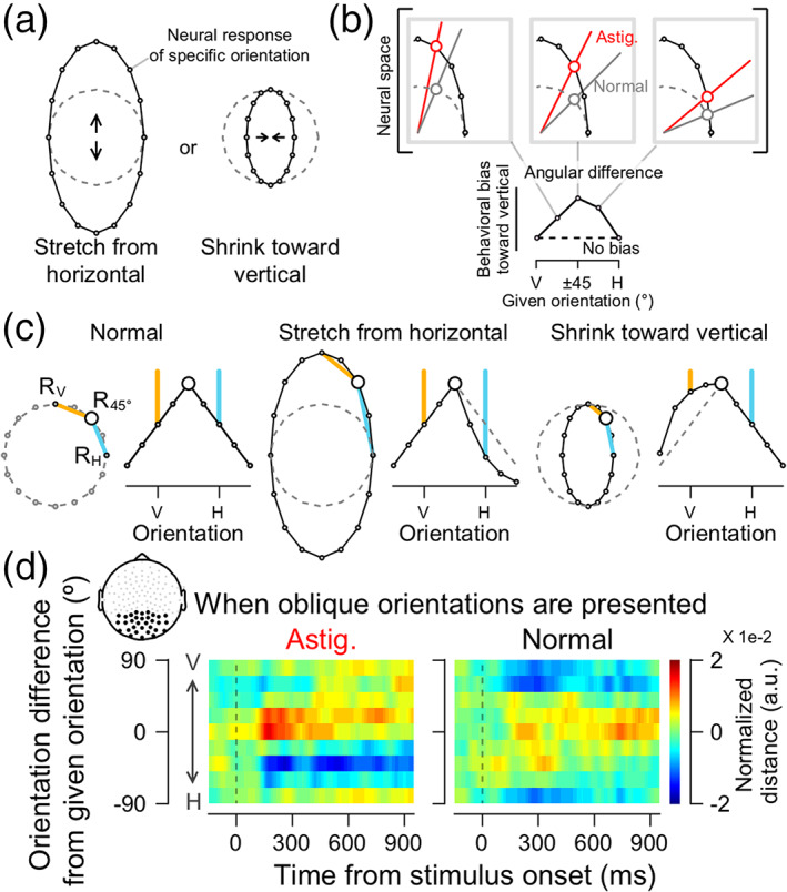
Distortion of orientation tuning responses in induced astigmatism. (a) Hypothetical shapes of the astigmatic distortion of the neural orientation space. The neural response of each stimulus orientation, represented as dots, would be circular in polar coordinates without systemic bias in the neural orientation space (dashed gray circles). In the astigmatic condition, the retinal distortion would produce a vertical oval neural orientation space. The oval shape can be formed either by stretching the space from the horizontal axis (left panel) or shrinking the space toward the vertical axis (right panel), or both. (b) In all possible scenarios, the observed behavioral bias pattern (bottom, from Figure 1c) can be obtained by measuring the angular distance between the orientation representations in the astigmatic (red lines in upper panels) and normal conditions (gray lines). (c) The expected shapes of decoded orientation tuning vector for each hypothesis when visual stimuli with oblique orientations are presented. The distances between neural responses to 45° orientation and those to other orientations (e.g., from R45° to R0° in orange lines, from R45° to R90° in sky‐blue lines) are arranged as a function of orientation differences from the given orientation, 45°. Then, it was turned upside‐down to obtain an orientation turning curve. In the normal condition (left panel), the length of orange and sky‐blue lines would be equal, forming a symmetrical tuning shape. On the other hand, if the orientation space is stretched away from the horizontal axis (middle panel), the distance to the horizontal axis (sky‐blue line) would be longer than usual, which would cause asymmetry in the tuning curve. If the orientation space is shrunken toward the vertical axis (right panel), the shortened distance to the vertical (orange line) causes asymmetry in the tuning by increasing the tuning values around the vertical axis. (d). Orientation tuning curves centered on oblique orientations in the astigmatic (left panel) and normal (right panel) conditions. The orientation tunings are measured for each oblique orientation (±22.5°, ±45°, ±67.5°) and averaged after rearranging the curves so that the distance from a given orientation to the vertical is plotted at the upper side of each panel. The upper left subfigure indicates the topography of posterior electrodes used in the analysis
In this study, we investigated the modulation of neural orientation representations induced by optical aberrations in astigmatism and how this modulation mediates perceptual errors. Specifically, we tested which characteristics of distortion in neural orientation representation the brain follows—either stretching away from the astigmatic axis or shrinkage toward the axis orthogonal to it. To achieve this purpose, we acquired electroencephalogram (EEG) activity from human participants while performing an orientation adjustment task in normal and induced astigmatic conditions. We estimated changes in the EEG response pattern as a function of stimulus orientation using a neural distance measure (Mahalanobis distance) and constructed an orientation tuning function. We first found that the orientation tuning responses were skewed away from the astigmatic axis in the induced astigmatic condition. The neural bias estimation in polar coordinates further verified that the neural orientation space had a vertically stretched elliptical shape (stretched away from the astigmatic axis), and that neural bias was predictive of behavioral astigmatic errors. Further, we performed cross‐temporal generalization analysis (CTG) to understand the underlying temporal dynamics of neural bias. The analysis revealed a transition in the temporal dynamics of the neural distortion, initially transient and dynamic, but later generalized and stable.
2. MATERIALS AND METHODS
2.1. Subjects
EEG and behavioral data were collected from 21 participants (14 male and 7 female, mean age 25.35 ± 4.05). One male participant was excluded from the study because of the poor quality of his EEG recordings (see below for specific criteria). The Institutional Review Board of Sungkyunkwan University and Public Institutional Bioethics Committee, designated by the Ministry of Health and Welfare, approved the study, and all participants provided written consent. All participants were naïve to the purpose of the experiment.
2.2. Experimental condition design
We administered a visual acuity test to all participants to ensure that their vision was normal. After identifying the dominant eye with monocular preference in binocular viewing (Purves & White, 1994), the monocular visual acuity test was performed on the dominant eye of all participants at a distance of 1 m using Early Treatment of Diabetic Retinopathy Study (ETDRS) charts on an iPad (Apple Inc., fourth generation, the maximum luminance of 374.2 cd/m2). Only participants with a vision >20/20 in their dominant eye participated in the experiment.
The experiments consisted of two conditions (induced astigmatic and normal). To simulate a myopic astigmatic state, we placed an additional +2.00 diopter cylindrical trial lens on the participant's dominant eye. The cylindrical lens placed additional refractive power selectively to a specific meridian, and it was critical to horizontally set the axis of the cylindrical lens (Figure 1a, red circle in front of the eye). The manipulation mimicked “with‐the‐rule astigmatism” because it exerted the maximum refractive power on the vertical meridians (Rabbetts, 2007, see fig. 5.4). This allowed light rays to pass through the vertical (sagittal) meridian to focus in front of the retina and vertically spread when reaching the retina (Figure 1a, red lines). In contrast, light rays passing through the horizontal (transverse) meridian adequately converged on the retina as a vertical line (Figure 1a, gray lines). Altogether, only horizontal information on the retina is blurred, vertically stretching the retinal image and image perception. Under normal conditions, we placed a Plano lens (+0.00 diopter lens) on the dominant eye for a fair comparison with the induced astigmatic condition.
Before setting the experimental conditions, we placed an additional spherical lens in front of the dominant eye to relax the ciliary muscle, thus making the crystalline lens thinnest; if the muscle was not relaxed to its maximum, the lens could thin more, so the eye could better adjust the retinal image. As it could nullify the axis‐specific blurring effect of the cylindrical lens in induced astigmatism, to prevent such adjustment, we used the fogging method to determine the spherical lens (Benjamin, 2006; see chapter 20, “Classic Fogging Technique” for details). We first blurred the vision by placing a +2.50 diopter spherical lens to the dominant eye (fogging); then, we reduced the power with a step size of 0.25, until the participant could read the Snellen chart on the screen at a distance of 60 cm (defogging). This procedure naturally yields a spherical diopter with the thinnest crystalline lens, ensuring that no further lens adjustment intervenes in the induction of astigmatic vision, while also automatically correcting the minor residual spherical errors that might remain in those with 20/20 vision (Benjamin, 2006; see table 20‐1). In the contralateral nondominant eye, we used a +10.00‐diopter spherical lens to prevent intervention in the dominant eye. The participants were instructed to keep both eyes open.
2.3. Stimuli and task design
Participants were instructed to judge the orientation of a tilted Gabor array presented on a gamma‐corrected CRT monitor (ViewSonic PF817, maximum and minimum luminance of 109.2 cd/m2 and 0.2 cd/m2, respectively, and gray background luminance 54.7 cd/m2) with a spatial resolution of 800 × 600 pixels and a vertical refresh rate of 100 Hz (Figure 1b). The experiments were conducted in a dark room with light from the monitor as the primary source of illumination. The presentation of visual stimuli was controlled by the Psychophysics Toolbox for MATLAB (Brainard, 1997; Pelli, 1997) running on a Mac mini. The subjects' viewing distance from the monitor was 60 cm. The experiment was initiated when each participant pressed a space bar. After 400 ms of the blank screen, twenty 0.25° radius Gabor stimuli were presented for 150 ms within the 2.5° radius of an invisible circular patch. Each Gabor inside an invisible circle was positioned randomly. The spatial frequency was two cycles per degree, and the luminance contrast was 60% (Michelson). We presented multiple small Gabor stimuli instead of one, a large Gabor stimulus for significant degradation of orientation information in the induced astigmatism while evoking strong EEG responses. The tilt angles of Gabor patches were randomly chosen from eight evenly spaced orientations (0°, ±22.5°, ±45°, ±67.5°, and 90°), and the orientations of all Gabors in the array were the same. After 800 ms of the poststimulus blank screen, a randomly oriented 5° radius white orientation bar appeared at the screen center, and participants were instructed to rotate the orientation bar by moving the mouse until it matched the perceived array orientation. They reported their decision by clicking the left mouse button within a time window of 2.8 s. During the trial, participants were asked to fixate their gaze at a 0.1° radius white fixation point.
The subjects completed five blocks of the normal and four blocks of the induced astigmatic condition. Each block contained 160 trials, and the block order randomized. Each orientation was presented with equal probability, and the order of orientations randomized. Participants were not informed of the condition or of their behavioral performance.
To test whether the perceptual error in the induced astigmatic condition was indeed astigmatic axis specific, we collected additional behavioral data from three male participants (Figure S1b). The task was identical except for the angle of the astigmatic axis, which was set to −45° instead of 90°. Each participant completed a total of 180 trials (10 repetitions of 18 orientations, from −90° to 80° with a step size of 10°).
2.4. Behavior analysis
We included only trials where the participants successfully reported their perceived orientation in the adjustment task. In addition, we rejected some trials due to sudden changes or noise in EEG activity; on average, only 1% of the trials were discarded because of the absence of responses, and the other 1% of the trials were discarded during EEG preprocessing, leaving 98% of the trials for further analysis. To quantify the distortion of orientation perception in the induced astigmatic condition, we calculated orientation biases in the following steps (Figure 1c). First, the participants' behavioral errors in the adjustment task were defined as the angular differences between the stimulus orientation and the reported orientation. A positive error indicated a clockwise response compared to the stimulus orientation, and a negative error a counter‐clockwise response. Second, the response errors in the normal condition were subtracted from those in the astigmatic condition because errors in the normal condition reflected individual intrinsic orientation preferences and biases such as cardinal bias (see Figure S1a for data before subtraction; Furmanski & Engel, 2000; Li, Peterson, & Freeman, 2006). Finally, to measure the astigmatic bias as a function of the absolute angular offset from the vertical axis, we flipped the signs of the errors with stimulus orientations between 0° and 90°. Then, data were combined according to the size of orientation offset from the vertical axis (e.g., trials with stimulus orientations of +22.5° and −22.5° were collapsed). For each collapsed orientation, we calculated the average orientation errors to measure the response bias toward the vertical axis. We used a circular statistics toolbox (Berens, 2009) for statistical analysis of all trigonometric values. To test whether the pattern of response bias change across orientations followed a specific shape, we performed trend analysis using one‐way ANOVA, comparing the changing pattern with a caret‐shaped trend.
2.5. Convolution model
To simulate the effect of induced astigmatism on retinal images, we built a simple convolution model (Figure S1c), mimicking the distortion of the retinal image by the cylindrical lens. We simulated the vertically stretched retinal image by convolving the original image with an oval‐shaped kernel. The convolution method, or point spread function, has been widely used and resembles the way each light ray of an image is stretched vertically (Figure 1a, compare the light ray before and after lens; Porter, Queener, Lin, Thorn, & Awwal, 2006, see section 10.6.2; Roorda, 2004, see fig. 2.6). Therefore, stimulus images () with different angles (0°, 22.5°, 45°, 67.5°, and 90°) were convolved () with an oval kernel shape (, horizontal radius and vertical radius ) to create a convolved image (). A particular pixel of at coordinates and , , is defined by Equation (1) below.
| (1) |
We decoded the orientation from the convolved Gabor image () by detecting pixel boundaries that changed color from white to black at the stimulus center. This decoding method was similar to the feature extraction computation performed on simple cells of the primary visual cortex optimized for edge detection (Hubel & Wiesel, 1959). The orientation of the line connecting the pixel boundaries was considered as the orientation of . A retinal bias induced by simulated astigmatism was obtained from the difference between the estimated orientation and the given orientation . As the degree of stretch varied from participant to participant (due to different eyeball sizes, the refractive power of the individual's crystalline lens, etc.), we used the ratio as a free parameter and estimated the best‐fitted oval shape kernel by minimizing the sum of squared errors between the estimated retinal bias and the behavioral response (Figure 1c, blue color). We used the simulated annealing algorithm in the global optimization toolbox in MATLAB (Mathworks Inc.) for the estimation procedure, and the ratio was bounded to a range between 0 and 50 so that the kernel could have a vertical (if >1) and horizontal oval shape (if <1). To evaluate if the kernel had an oval shape, we tested if the estimated ratio was significantly different from one (which indicates no distortion) using a one‐sample t‐test.
2.6. EEG data acquisition and preprocessing
EEG data were collected from a 128‐sensor HydroCel “Sensor Nets” (Electrical Geodesics, Eugene OR), with a sampling rate of 500 Hz. Before recording, the impedances of all electrodes were lowered below 50 kΩ by administering potassium chloride solutions (average impedance across all electrodes and participants was 17.53 ± 3.19 kΩ), and checked and re‐lowered on every block (approximately every 10 min). To record the actual stimulus onset timing and to count any delay or temporal jitter induced by the monitor refresh, we used a photodiode to detect flashings of a small white square located at the top‐left region of the monitor at the time of stimulus onset in each trial.
The acquired EEG data were preprocessed through subroutines of EEGlab (Delorme & Makeig, 2004), FASTER (Nolan, Whelan, & Reilly, 2010), and FieldTrip toolbox (Oostenveld, Fries, Maris, & Schoffelen, 2011), following the steps described onward. First, EEG data were epoched from −1,000 to 1,950 ms relative to the stimulus onset marked by the photodiode event timestamp. Then, data were filtered with a band‐pass filter (from 0.3 to 200 Hz), and line noise removed using a notch filter (60 Hz, from 58 to 62 Hz). After re‐referencing all data using the average as the reference (Bigdely‐Shamlo, Mullen, Kothe, Su, & Robbins, 2015), independent component analysis (ICA; Makeig, Jung, Bell, & Sejnowski, 1996) was performed to identify and remove artifactual components induced by unwanted eye movements or blinks. For a fair comparison between conditions, EEG data were fed into the ICA, regardless of the condition. If the rejected ICs' total sum of explained variance >50%, the participant's data were rejected. One participant's data were discarded because 78.7% of the data were rejected after the preprocessing procedure. In the remaining participants' data, 7.5 ICs (explained 30.1% of data variance) were rejected on average. Data were then corrected to baseline by subtracting the average signal between −200 and −50 ms relative to stimulus onset in each channel and individual trials. Baseline‐corrected data were further smoothed by a sliding time window of 40 ms every 2 ms. Finally, to prevent a few noisy channels from dominating the entire activity pattern, the signal was normalized with the standard deviations across trials at each time point and electrode.
In the current study, we mainly used EEG data from the posterior channels for further analysis (33 electrodes around Pz and Oz) because the induced astigmatism was dominant in visual perception. Three other regions of interest (ROIs), based on EEG electrode locations on the scalp, were also compared (Figure S3b): anterior electrodes (28 around the Fz), electrodes around a vertex (32 around the Cz), and eye movement‐related electrodes (16 around the eyes).
2.7. Estimation of orientation tuning response
To decode the orientation information from the multivariate EEG activity pattern, we first calculated the Mahalanobis distances between neural activity patterns to different stimulus orientations. Then, we converted them into distance vectors, which are conceptually similar to an orientation tuning curve (Myers et al., 2015; Wolff, Ding, Myers, & Stokes, 2015; Wolff, Jochim, Akyürek, & Stokes, 2017). In each trial (and at each time point), we computed the Mahalanobis distances between the current trial's multivariate EEG activity and multivariate EEG activity averages (across trials) in eight orientations (excluding the current trial), then arranged them as a 1‐by‐8 vector. The distance to its own orientation was arranged to be at the center of the vector, and those to other orientations were set apart from the center according to the differences from the current (test) orientation (zero‐centering to the test orientation). We estimated the covariance matrix for the Mahalanobis distance computation from all except for the given trial using a shrinkage estimation method (Ledoit & Wolf, 2004). To ensure the robustness of the distance vector, we performed permutation analysis. We generated a null distribution of the estimated distance vectors by shuffling the trial‐wise mapping between the EEG response and given stimulus orientation 500 times. We then transformed the original distance vector into standard scores (Z‐score) by subtracting the mean of the null distribution and dividing it by the standard deviation of the null distribution. If orientation responses of multivariate EEG activity patterns followed the parametric circular space (Figure 2c, left panel), the distance vector would follow a V shape; the center vector components, representing the distance to the current trial's own orientation, would be the smallest and gradually increase as the orientation of each vector component becomes distant. Finally, we obtained the orientation tuning curves by subtracting the means of distance vectors across orientations and reversing the sign. If the test orientation was −67.5°, −45°, and −22.5°, we used a mirror image of the orientation tuning curves before combining them with those from other orientations. The aim was to maintain the distance‐vector component of the vertical axis at the left side of the center, regardless of the test orientation. To evaluate the significance of the orientation tuning from the distance vectors, we measured the cosine amplitudes of the orientation tuning curve by convolving it with a cosine kernel, cos (2θ) (Wolff et al., 2017), where is a vector of the orientation difference from the given orientation, arranged as previously described (θ = [−90°, −67.5°, −45°, −22.5°, 0°, 22.5°, 45°, 67.5°]).
2.8. Estimation of neural bias
We measured the neural bias by comparing the regularities of the orientation space obtained from the Mahalanobis distance in the induced astigmatic and normal conditions. If the astigmatic distortion would stretch or shrink the circular orientation representations, the neural distances between the horizontal axis and nearby orientations, or the distances between the vertical axis and nearby orientations would differ between the two conditions (Figure 3a). Therefore, we first calculated the Mahalanobis distances between the EEG response to a specific orientation and a nearby orientation ().
| (2) |
where is the multivariate EEG response to stimulus orientation θ i at a particular time point , shows the Mahalanobis distance between A and B, and α j represents a nearby orientation away from θ i (, orange and sky‐blue lines in Figure 3a). Next, we subtracted the average of all possible s from to test whether the neural distance from a nearby orientation α j to the reference orientation (horizontal or vertical axes) was significantly different from others in the orientation space (, the number of orientations, n = 8).
| (3) |
Note that, this scaling procedure automatically eliminated distance differences among αj ( was more likely to be larger than before scaling). If the neural orientation representations would have a uniform circular shape (without any distortions around the vertical or horizontal axis), as expected in the normal condition, the average across all nearby orientations would remain zero (, Figure S3a; orange and sky‐blue lines have the same length). Finally, we calculated the neural bias around a specific orientation (horizontal axis or vertical axis) by subtracting in the normal condition from in the induced astigmatic condition and averaged them across all six nearby orientations (Figure 3a; the length difference between orange and sky‐blue lines in each panel, , the number of nearby orientations, m = 6).
| (4) |
| (5) |
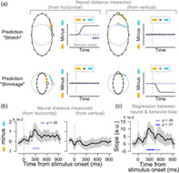
FIGURE 3.
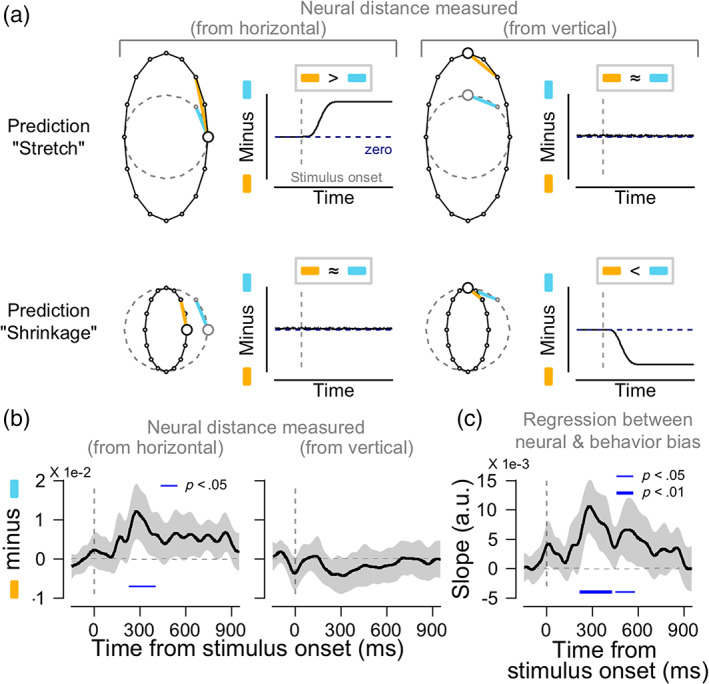
Neural bias under the astigmatic condition. (a). Predicted patterns of neural biases for each hypothesis. If the astigmatic distortion stretches the circular orientation representations away from the horizontal axis (“stretch from the horizontal” hypothesis), the neural distance measured from the horizontal to other oblique orientations in the astigmatic condition would be larger than that in the normal condition (neural bias measured from the horizontal to be positive after stimulus onset, upper left panel, the difference between the orange and sky‐blue lines). Meanwhile, the neural distance measured from the vertical would not differ across conditions (upper right panel). If the astigmatic distortion shrinks the circular representations toward the vertical axis (“shrinkage toward the vertical” hypothesis), the neural distances measured from the horizontal to oblique orientations will remain zero (lower left panel), while the distance measured from the vertical to oblique orientations would be smaller than that in the normal condition (the neural bias would be negative values, lower right panel). (b). Neural bias measured from the horizontal (left panel) and the vertical (right panel) axes from posterior electrodes. (b and c) Shaded ribbons indicate ±2 SEM, and solid blue lines at the bottom significant time clusters (thin lines, p <.05; thick line p <.01). (c). The association between the neural biases and perceptual errors is estimated from regression analysis
denotes the average neural bias around the horizontal axis across the six nearby orientations, is the scaled neural distance from a nearby orientation to the horizontal axis in the astigmatic condition, and is the scaled neural distance from to the horizontal axis in the normal condition, measured at a particular time point (Figure 3a, left panels; orange minus sky‐blue lines). We calculated the neural bias around the vertical axis, in a similar way (Figure 3a, right panels; orange minus sky‐blue lines). The resulting measures were further smoothed using a Gaussian smoothing kernel with an SD of 20 ms.
Here, we estimated the neural bias by comparing the neural distances across astigmatism conditions after scaling them within each condition, rather than calculating neural distances across conditions first and then scaling them later. We avoided the latter approach to prevent factors that differed under astigmatism conditions but were not directly related to the orientation information, from affecting the result (e.g., the difference in the retinal input strength, the task difficulty, or subsequent levels of attention).
To test if the measured distortion in the neural orientation space significantly impacted perceptual error, we quantified the association between the two using linear regression analysis (Figure 3c). We plotted the mean behavioral response biases toward the vertical axis in oblique orientations () as a function of the scaled neural distances between the horizontal axis and the oblique, nearby orientations ( from Equation (4)). We then estimated the slopes of the linear regression and reported them as a function of time.
2.9. CTG analysis of neural bias
To understand the underlying temporal characteristics of neural dynamics in induced astigmatism, we used CTG analysis (King & Dehaene, 2014). In this analysis, all other procedures for estimating the neural bias were identical to the method described above; only the selection of multivariate EEG activity patterns used for computing Mahalanobis distance were different. We computed the Mahalanobis distance between the two multivariate EEG activity patterns selected from different times, that is, the distance between the EEG responses to the horizontal axis at a reference time point and those to the oblique orientations () at another time point (Figure 4).
| (6) |
| (7) |
| (8) |
Note that the current CTG analysis connotes temporal directionality because and are not identical. The CTG matrix for the neural bias measured from the vertical axis () was also computed using an identical procedure, except that was used instead of (Figure S4).
FIGURE 4.

Cross‐temporal generalization (CTG) analysis of neural bias measured from the horizontal axis. The analysis directly tests whether the astigmatic stretch at the reference time point (t ref) is generalizable to other time points (t k). As in Figure 3, neural bias (left panel) is obtained by subtracting the scaled neural distance measured from the horizontal to other oblique orientations in the normal vision condition (right panel) from that in the astigmatic vision condition (middle panel). The only difference is that neural responses to the horizontal axis were measured at t ref and those to the oblique orientations are measured at another time point t k, resulting in a 2D matrix form in each panel. Red (blue) values indicate larger (smaller) neural bias around the horizontal axis. The two subfigures on the right side of the neural bias are zoom‐ins of the black squares in the main figure. Each black square shows the dynamic period (upper subfigure) and stable period (lower subfigure), respectively. Example data points of t ref, t k, and their across‐time comparison are marked as a–c and a′–c′. The black contoured area shows a significant time cluster, where neural biases are different from zero (cluster‐based permutation t‐test, p = .002)
2.10. Methodological consideration and statistical testing
Recent studies have emphasized the importance of setting proper references to obtain robust and reliable results. Some studies suggested more elaborate techniques for setting references (for example, reference electrode standardization technique, REST; Yao, 2001) than other standard techniques, such as the common average reference technique that we used in this study (Bigdely‐Shamlo et al., 2015). Although reference selection can have substantial effects on EEG amplitudes, it was not critical in our study because our main conclusion arises from the relative comparisons of spatially distributed EEG activity patterns across different conditions.
To address the multiple comparison problem in the neural indices (amplitudes of decoded orientation tuning, neural biases, and CTG analysis), we corrected the statistical criterion (p‐value) of the two‐tailed, one‐sample t‐test with a nonparametric, cluster‐based permutation approach using a statistical toolbox in MATLAB (Maris & Oostenveld, 2007). Based on the assumption that temporally close data points are correlated, significant time clusters were selected when the p‐values of the successive t‐values were <0.05, and the sum of t‐values in each time cluster was computed. Next, for each time cluster, the null distribution of summed t‐values was computed through random data shuffling with zeros (3,000 times) because we wanted to test if the time clusters of the neural indices were significantly different from zero. The final corrected p‐values were determined by the percentile of the original summed t‐value in the null distribution. Time clusters with corrected p‐values <.05 were considered statistically significant.
3. RESULTS
3.1. Induced astigmatism biases behavioral responses following retinal bias
Human participants were asked to report the perceived orientation of tilted Gabor stimuli in normal and induced astigmatic vision conditions (Figure 1b). Astigmatic vision was simulated by applying a cylindrical lens with the axis set to the horizontal (astigmatic axis, “with‐the‐rule astigmatism,” Figure 1a, red circle). Based on the nature of simulated astigmatism, the orientation information in the retinal image would be biased toward the vertical axis when Gabor arrays with oblique orientations were presented, but the orientation information would be intact when Gabors with cardinal orientations were presented (see Figure S1c, for example of retinal images).
Consistent with the predicted retinal distortion, the perceptual error toward the vertical axis increased as the given orientation approached ±45° and decreased as the stimulus orientation approached the horizontal axis (Figure 1c, red line). This distinct change pattern in perceptual error was statistically significant (caret‐shaped [^] trend for perceptual error, trend analysis, F (4,76) = 31.159, p <1e−6). In an additional control experiment, we changed the lens axis from horizontal to −45° to exclude the effect of other axis‐specific factors, such as the cardinal bias in perception (Furmanski & Engel, 2000; Li et al., 2006). The caret‐shaped trend of the perceptual error was maintained regardless of whether we set the lens axis to horizontal or −45°. To further test how much of the observed perceptual error was explained by the predicted retinal distortion, we simulated the astigmatic aberration by convolving the 2D retinal image of oriented Gabor stimuli with an oval shape kernel (Figure S1c, Porter et al., 2006, see section 10.6.2; Roorda, 2004, see fig. 2.6, for an example). We estimated the model parameter (r) that adjusted the amount of vertical or horizontal image stretches by fitting the predicted perceptual errors from the model to the behavioral data (see Section 2 for more details). The model could explain the behavioral data (Figure 1c, in blue), suggesting that the behavioral error in the induced astigmatism mainly originates from the low‐level distortion of the retinal image (model explained variance 58.8 ± 15.5%; = 5.6 ± 0.7, one‐sample t‐test with one, t 19 = 12.776, p <1e−10).
3.2. Induced astigmatism skewed neural orientation tuning responses
Next, we investigated how retinal distortion modulated the neural representation of orientation. Under normal conditions, the neural tuning curves constructed from multivariate EEG responses to oblique orientation Gabor stimuli would be symmetric in a circular neural orientation space (Figure 2c, left panel). In the astigmatic condition, the “stretch from the horizontal” hypothesis predicts that values of neural tuning for orientations close to the horizontal axis would be lower (Figure 2c, sky‐blue line in the middle panel). On the other hand, the “shrinkage toward the vertical” hypothesis predicts higher tuning values for orientations close to the vertical axis (Figure 2c, orange line in the right panel).
The estimated neural orientation tuning curve in the astigmatic condition was skewed away from the horizontal axis (Figure 2d, left panel) while tuning in the normal condition was symmetric (Figure 2d, right panel). The values of the tuning function close to the horizontal axis were lower (the lower side of Figure 2d, left panel), and those close to the vertical axis higher (the upper side of Figure 2d, left panel) than those in the normal condition. The specific pattern of the change in the astigmatic condition appears to support the “stretch from the horizontal” hypothesis, as the decrease close to the horizontal axis was more pronounced and lasted longer. The tuning curves from the responses to the orientations near the cardinals (horizontal and vertical axes) also showed the expected distortion, even if perceptual errors were minimal (Figure S2b).
3.3. Quantification of the neural bias in the orientation space
So far, we showed that the neural orientation space in induced astigmatism was distorted consistently with the prediction of the “stretch from the horizontal” hypothesis. To perform a quantitative measure of the distortion and evaluate how these distorted orientation representations are linked to behavioral errors, we first quantified the robustness of tuning responses using cosine amplitude (Wolff et al., 2017). In the normal condition, the tuning functions were significant most of the time regardless of the presented stimulus orientation (Figure S2c, second and fourth panel). However, in the induced astigmatism condition, the significance of tuning responses depended on the presented orientation: it was barely significant with oblique orientation stimuli but showed more robust orientation responses with cardinal orientation stimuli (Figure S2c, first and third panel). Although we found a dependency of tuning responses on the specific stimulus orientation in the induced astigmatism, we could not distinguish whether the weak cosine amplitudes for responses to oblique orientations were due to the skew in orientation tuning functions or to the overall weak orientation responses.
To overcome this limitation of conventional methods, we estimated the “neural bias” by directly measuring the extent of stretching from or shrinking toward a specific axis of the neural orientation space in the astigmatic condition and compared it to normal conditions (orange lines minus sky‐blue lines, see Section 2 for details). If the neural orientation space was stretched away from the horizontal axis, the neural distances from the horizontal axis to the oblique orientations would be larger in the astigmatic condition than in the normal condition (Figure 3a, upper left panel; compare the length of orange and sky‐blue lines), and the distances from vertical to oblique would remain relatively similar across conditions (Figure 3a, upper right panel). If the neural orientation space shrunk toward the vertical axis, the neural distance from the vertical to the oblique orientations would be smaller in the astigmatic than in the normal condition (Figure 3a, lower right panel). In contrast, the distance from the horizontal to the oblique orientations would be similar across the conditions (Figure 3a, lower left panel).
When we measured the neural bias from the horizontal axis, it was transiently and significantly increased after stimulus onset (Figure 3b, left panel, cluster‐based permutation test, from 228 to 404 ms relative to the stimulus onset, p = .017) and continued generally positive. The average neural bias calculated from the vertical axis, on the other hand, remained close to zero during the trial (Figure 3b, right panel). Therefore, we concluded that the neural orientation space was vertically stretched as if the neural responses to oblique orientations were repelled away from the responses to the horizontal axis, which is the axis of maximum refractive power in the cylindrical lens we used to induce astigmatism. Systematic distortion of the neural space was only observed in the EEG activity from posterior channels. We could not find any distortion from EEG activity in different ROIs, including the anterior channels (Figure S3b). This suggests that perceptual error under induced astigmatism mainly originates from the posterior regions of the brain.
Finally, we tested whether this significant distortion in the neural orientation space was predictive of behavioral errors in induced astigmatism. To find the association, we performed a linear regression analysis for each participant, using the neural bias measured from the horizontal axis (six oblique orientations: ±22.5°, ±45°, and ±67.5°) as an independent variable and perceptual error of corresponding orientations as a dependent variable (see Section 2 for details). The regression slopes were significantly positive across participants at the time when neural biases were significant (Figure 3c, cluster‐based permutation test, from 216 to 428 ms relative to the stimulus onset, p = .009) and lasted for another 100 ms (from 452 to 580 ms, p = .035). This result is important because it suggests that the observed distortion in the neural orientation space mediates the perceptual error and affects the participant's orientation judgment.
3.4. Underlying neural dynamics revealed from CTG analysis
Since the distortion in the neural orientation space is meaningful for perceptual decision, we further investigated the temporal neural dynamics of the neural distortion using CTG analysis (King & Dehaene, 2014). The analysis showed how far the stretch around the horizontal axis in the neural orientation space would be generalized in time. To this end, we estimated the neural bias not only within each time point, but also across time points. For each condition, the distances were measured between the multivariate EEG responses to the horizontal axis at a reference time point and that to oblique orientations at another time point. As a result, distances were computed in a two‐dimensional matrix form (number of reference time points by number of time points to be compared). Again, the distance matrix obtained under normal conditions (Figure 4, right panel) was subtracted from the matrix in the astigmatic condition (middle panel) to obtain a CTG matrix of neural bias (left panel, see Section 2 for details, especially Equations (6)–(8)). If the pattern of neural response keeps changing, the vertical stretch of the orientation space would differ from time to time, and the neural bias would only be significant at the diagonal of the CTG matrix (compare a and b with c in Figure 4, lower subfigure). If the neural orientation space was stable across time, the neural biases at each time point could be generalized across different time points and significantly at the off‐diagonal of CTG (see a′, b′, and c′ in the upper subfigure).
We found an interesting pattern of generalization. The oval shape neural orientation space was initially temporally dynamic (up to 350 ms from stimulus onset) but later stabilized (cluster‐based permutation test, p = .002). We could not find a significant CTG map when measuring the neural bias from the vertical axis (Figure S4). This again confirms that the distortion of the neural orientation space by astigmatism follows the prediction of the “stretch from the horizontal” hypothesis.
4. DISCUSSION
In this study, we investigated the neural underpinnings of systematic perceptual errors in astigmatic vision. We estimated the neural orientation space from multivariate EEG activity patterns and found that it was systematically distorted in a way that supported the orientation perception errors: the orientation space was maximally stretched away from the astigmatic axis where the blurring of the stimulus orientation was at the maximum, while the space around the axis orthogonal to the astigmatic axis where the effect of the blurring was minimal was intact. The distortion in the neural orientation space was capable of explaining the pattern of behavioral error in orientation perception, and the degree of neural distortion correlated with the size of the perceptual error.
The current study expanded the previous literature by demonstrating how axis‐specific optical aberration in astigmatism modulates neural orientation representation. In previous studies, the primary goal of measuring neural activity was to detect immediate abnormal blur. Thus, they focused on measuring the attenuation and delay in transient EEG activity that mainly reflects the stimulus' physical properties, such as contrast change (P1 component of event‐related potentials, or ERPs, peaks around 100 ms relative to the stimulus onset; Anand et al., 2011; Bobak et al., 1987; May et al., 1979; Regan, 1973; Sokol, 1983). The current experiment replicated the difference in ERP activity between the normal and astigmatic conditions in the early period (Figure 5, from 106 to 170 ms and from 114 to 170 ms relative to the stimulus onset, Oz and Fz, respectively; cluster‐based permutation test, = .027, = .048). However, these results do not directly demonstrate how immediate optical blur alters the neural orientation representation and results in perceptual errors. In fact, the timing of ERP differences (P1 component) is quite early compared to the appearance of the neural bias relevant to the astigmatic orientation perception (from 228 ms relative to the stimulus onset to the end of trial; Figures 3 and 4). This suggests the existence of a distinct temporal sequence in the underlying neural processes for the immediate optical blur and the resulting distortion in orientation perception.
FIGURE 5.

Normalized event‐related potential (ERP) to Gabor stimuli in astigmatic (red) or normal conditions (black), for electrodes OZ (left panel), PZ (middle panel), and FZ (right panel). The subfigures above indicate the spatial position of each electrode
We also showed a conspicuous temporal transition in information processes by analyzing the temporal dynamics of astigmatic distortion in the neural orientation space. In the initial phase of the EEG responses, the vertically stretched neural orientation spaces dynamically changed from moment to moment. Later, the oval‐shaped orientation space stabilized over time. Although it is not clear how the transition in temporal dynamics occurred, one possibility lies in the timing of the distortion transition. Early EEG waves are typically regarded as a reaction to the physical properties of a given stimulus, and later waves are considered to be involved in cognitive information processes such as stimulus evaluation (Polich, 2007) or working memory (Vogel & Machizawa, 2004). Therefore, the initial orientation‐related neural responses might be responsible for the early dynamical changes, while later neural activity might be responsible for the stable maintenance of the distorted orientation space. What seems peculiar is the relatively long stable phase of the “neural trace” for visual stimuli in EEG responses, even in the absence of stimuli (note that the stimulus was turned off after 150 ms from onset).
Given that the neural representation does not necessarily exist in explicit form but in “activity‐silent” states after the initial response periods (Stokes, 2015; Wolff et al., 2015, 2017), the explicitly maintained neural distortion in the later period might indicate the involvement of extra‐retinal factors besides the direct feedforward inputs. Various cognitive factors may modify orientation perception under astigmatism. For example, blur detection on specific meridians may increase visual attention, or exposure to the astigmatic condition (short‐term or long‐term experience) may allow the participants to build prior expectations, which could contribute to the neural bias for a specific orientation. In this study, however, we could not find strong support for the involvement of the extra‐retinal component in orientation perception under astigmatism. Significant neural orientation distortion was observed only in the posterior channels (those close to the visual cortex). We should note that the lack of support for cognitive factor involvement might be partly due to our experimental design or analysis methods. Our method for quantifying distortion in the orientation space was robust and conservative, which might have resulted in the failure to detect subtle but significant changes. Future research may show the involvement of other brain regions, including the frontal cortex, by investigating the role of higher cognitive functions in astigmatic visual perception.
The current study serves as a foundation to expand our understanding of the underlying neural processes of astigmatic perception. Growing evidence suggests an active role for neural compensation in astigmatism. Numerous behavioral studies have shown that visual acuity is improved after exposure to natural or induced astigmatism for a long time, even if the optical aberration is uncorrected (de Gracia, Dorronsoro, Marin, Hernandez, & Marcos, 2011; Ohlendorf, Tabernero, & Schaeffel, 2011; Sawides, de Gracia, Dorronsoro, Webster, & Marcos, 2011; Sawides et al., 2010; Vinas, Sawides, de Gracia, & Marcos, 2012). Several studies have suggested the possibility of neural compensation in astigmatic distortions and proposed solutions in various contexts, such as neural modification of optical aberrations (Chen, Artal, Gutierrez, & Williams, 2007; Webster, Georgeson, & Webster, 2002), neural plasticity to mitigate optical blur (Flitcroft, 2012; Pons et al., 2019), and adjustment of the focal point during eyeball growth (Troilo, 1990; Wallman, 1993; Wildsoet, 2003). Despite the behavioral evidence, direct measurements of neural activity and investigations on the neural mechanisms for astigmatism are rare. The current study presents how the distinct characteristics of astigmatism can be systematically studied in the neural domain. Based on the current study, future research may reveal how neural processing compensates for distorted retinal images, especially when the visual system is chronically exposed to astigmatism.
CONFLICT OF INTEREST
The authors declare no competing financial interests.
AUTHOR CONTRIBUTIONS
Joonsik Moon, Sangkyu Son, Hyungoo Kang, and Yee‐Joon Kim: Conceptualization; Sangkyu Son, Joonsik Moon, Hyungoo Kang, Yee‐Joon Kim, and Joonyeol Lee: Methodology; Sangkyu Son and Joonsik Moon: Investigation; Sangkyu Son and Joonyeol Lee: Formal analysis; Sangkyu Son and Joonyeol Lee: Writing—original draft; Sangkyu Son, Joonsik Moon, Hyungoo Kang, Yee‐Joon Kim, and Joonyeol Lee: Writing—review and editing; Yee‐Joon Kim, and Joonyeol Lee: Funding acquisition.
Supporting information
Appendix S1: Supporting Information
ACKNOWLEDGMENTS
The authors thank Dr. Preeti Verghese and Won Mok Shim for constructive comments on earlier versions of this manuscript. This research was supported by IBS‐R015‐D1, IBS‐R001‐D1 and IBS‐R001‐D2.
Son, S., Moon, J., Kang, H., Kim, Y.‐J., & Lee, J. (2021). Induced astigmatism biases the orientation information represented in multivariate electroencephalogram activities. Human Brain Mapping, 42(13), 4336–4347. 10.1002/hbm.25550
Sangkyu Son and Joonsik Moon authors contributed equally to this work.
Funding information Institute for Basic Science, Grant/Award Numbers: R001‐D1, R001‐D2, R015‐D1
Contributor Information
Yee‐Joon Kim, Email: joon@ibs.re.kr.
Joonyeol Lee, Email: joonyeol@g.skku.edu.
DATA AVAILABILITY STATEMENT
The data that support the findings of this study are available from the corresponding author upon reasonable request.
REFERENCES
- Anand, A., De Moraes, C. G. V., Teng, C. C., Liebmann, J. M., Ritch, R., & Tello, C. (2011). Short‐duration transient visual evoked potential for objective measurement of refractive errors. Documenta Ophthalmologica, 123(3), 141–147. [DOI] [PubMed] [Google Scholar]
- Atchison, D. A., & Mathur, A. (2011). Visual acuity with astigmatic blur. Optometry and Vision Science, 88(7), E798–E805. [DOI] [PubMed] [Google Scholar]
- Attebo, K., Ivers, R. Q., & Mitchell, P. (1999). Refractive errors in an older population: The blue mountains eye study. Ophthalmology, 106(6), 1066–1072. 10.1016/S0161-6420(99)90251-8 [DOI] [PubMed] [Google Scholar]
- Benjamin, W. J. (2006). Borish's clinical refraction. Amsterdam, The Netherlands: Elsevier Health Sciences. [Google Scholar]
- Berens, P. (2009). CircStat: A MATLAB toolbox for circular statistics. Journal of Statistical Software, 31(10), 1–21. 10.1002/wics.10 [DOI] [Google Scholar]
- Bigdely‐Shamlo, N., Mullen, T., Kothe, C., Su, K.‐M., & Robbins, K. A. (2015). The PREP pipeline: Standardized preprocessing for large‐scale EEG analysis. Frontiers in Neuroinformatics, 9(June), 1–20. 10.3389/fninf.2015.00016 [DOI] [PMC free article] [PubMed] [Google Scholar]
- Bobak, P., Bodis‐Wollner, I., & Guillory, S. (1987). The effect of blur and contrast of VEP latency: Comparison between check and sinusoidal grating patterns. Electroencephalography and Clinical Neurophysiology/Evoked Potentials Section, 68(4), 247–255. [DOI] [PubMed] [Google Scholar]
- Bradley, A., Thomas, T., Kalaher, M., & Hoerres, M. (1991). Effects of spherical and astigmatic defocus on acuity and contrast sensitivity: A comparison of three clinical charts. Optometry and Vision Science, 68(6), 418–426. [DOI] [PubMed] [Google Scholar]
- Brainard, D. H. (1997). The psychophysics toolbox. Spatial Vision, 10(4), 433–436. 10.1163/156856897X00357 [DOI] [PubMed] [Google Scholar]
- Chen, L., Artal, P., Gutierrez, D., & Williams, D. R. (2007). Neural compensation for the best aberration correction. Journal of Vision, 7(10), 9–9.9. [DOI] [PubMed] [Google Scholar]
- de Gracia, P., Dorronsoro, C., Marin, G., Hernandez, M., & Marcos, S. (2011). Visual acuity under combined astigmatism and coma: Optical and neural adaptation effects. Journal of Vision, 11(2), 5–5. 10.1167/11.2.5 [DOI] [PubMed] [Google Scholar]
- Delorme, A., & Makeig, S. (2004). EEGLAB: An open source toolbox for analysis of single‐trial EEG dynamics including independent component analysis. Journal of Neuroscience Methods, 134(1), 9–21. 10.1016/j.jneumeth.2003.10.009 [DOI] [PubMed] [Google Scholar]
- Flitcroft, D. I. (2012). The complex interactions of retinal, optical and environmental factors in myopia aetiology. Progress in Retinal and Eye Research, 31(6), 622–660. [DOI] [PubMed] [Google Scholar]
- Furmanski, C. S., & Engel, S. A. (2000). An oblique effect in human primary visual cortex. Nature Neuroscience, 3(6), 535–536. 10.1038/75702 [DOI] [PubMed] [Google Scholar]
- Guo, H., & Atchison, D. A. (2010). Subjective blur limits for cylinder. Optometry and Vision Science, 87(8), E549–E559. 10.1097/OPX.0b013e3181e61b8f [DOI] [PubMed] [Google Scholar]
- Hubel, D. H., & Wiesel, T. N. (1959). Receptive fields of single neurones in the cat's striate cortex. The Journal of Physiology, 148(3), 574–591. 10.1113/jphysiol.1959.sp006308 [DOI] [PMC free article] [PubMed] [Google Scholar]
- King, J. R., & Dehaene, S. (2014). Characterizing the dynamics of mental representations: The temporal generalization method. Trends in Cognitive Sciences, 18(4), 203–210. 10.1016/j.tics.2014.01.002 [DOI] [PMC free article] [PubMed] [Google Scholar]
- Kobashi, H., Kamiya, K., Shimizu, K., Kawamorita, T., & Uozato, H. (2012). Effect of axis orientation on visual performance in astigmatic eyes. Journal of Cataract & Refractive Surgery, 38(8), 1352–1359. 10.1016/j.jcrs.2012.03.032 [DOI] [PubMed] [Google Scholar]
- Ledoit, O., & Wolf, M. (2004). Honey, I shrunk the sample covariance matrix. The Journal of Portfolio Management, 30(4), 110–119. 10.3905/jpm.2004.110 [DOI] [Google Scholar]
- Li, B., Peterson, M. R., & Freeman, R. D. (2006). Oblique effect: A neural basis in the visual cortex. Journal of Neurophysiology, 90(1), 204–217. 10.1152/jn.00954.2002 [DOI] [PubMed] [Google Scholar]
- Makeig, S., Jung, T.‐P., Bell, A. J., & Sejnowski, T. J. (1996). Independent component analysis of electroencephalographic data. Advances in Neural Information Processing Systems, 3, 145–151. [Google Scholar]
- Maris, E., & Oostenveld, R. (2007). Nonparametric statistical testing of EEG‐ and MEG‐data. Journal of Neuroscience Methods, 164(1), 177–190. 10.1016/j.jneumeth.2007.03.024 [DOI] [PubMed] [Google Scholar]
- May, J. G., Cullen, J. K., Jr., Moskowitz‐Cook, A., & Siegfried, J. B. (1979). Effects of meridional variation on steady‐state visual evoked potentials. Vision Research, 19(12), 1395–1401. [DOI] [PubMed] [Google Scholar]
- Myers, N. E., Rohenkohl, G., Wyart, V., Woolrich, M. W., Nobre, A. C., & Stokes, M. G. (2015). Testing sensory evidence against mnemonic templates. ELife, 4(DECEMBER2015), 1–25. 10.7554/eLife.09000 [DOI] [PMC free article] [PubMed] [Google Scholar]
- Nolan, H., Whelan, R., & Reilly, R. B. (2010). FASTER: Fully automated statistical thresholding for EEG artifact rejection. Journal of Neuroscience Methods, 192(1), 152–162. 10.1016/j.jneumeth.2010.07.015 [DOI] [PubMed] [Google Scholar]
- Ohlendorf, A., Tabernero, J., & Schaeffel, F. (2011). Neuronal adaptation to simulated and optically‐induced astigmatic defocus. Vision Research, 51(6), 529–534. 10.1016/j.visres.2011.01.010 [DOI] [PubMed] [Google Scholar]
- Oostenveld, R., Fries, P., Maris, E., & Schoffelen, J.‐M. (2011). FieldTrip: Open source software for advanced analysis of MEG, EEG, and invasive electrophysiological data. Computational Intelligence and Neuroscience, 2011, 156869–156869. 10.1155/2011/156869 [DOI] [PMC free article] [PubMed] [Google Scholar]
- Pelli, D. G. (1997). The VideoToolbox software for visual psychophysics: Transforming numbers into movies. Spatial Vision, 10, 437–442. [PubMed] [Google Scholar]
- Polich, J. (2007). Updating P300: An integrative theory of P3a and P3b. Clinical Neurophysiology, 118(10), 2128–2148. 10.1016/j.clinph.2007.04.019 [DOI] [PMC free article] [PubMed] [Google Scholar]
- Pons, C., Jin, J., Mazade, R., Dul, M., Zaidi, Q., & Alonso, J.‐M. (2019). Amblyopia affects the ON visual pathway more than the OFF. Journal of Neuroscience, 39(32), 6276–6290. [DOI] [PMC free article] [PubMed] [Google Scholar]
- Porter, J., Queener, H., Lin, J., Thorn, K., & Awwal, A. A. S. (2006). Adaptive optics for vision science: Principles, practices, design, and applications (Vol. 171). Hoboken, NJ: John Wiley & Sons. [Google Scholar]
- Purves, D., & White, L. E. (1994). Monocular preferences in binocular viewing. Proceedings of the National Academy of Sciences, 91(18), 8339–8342. 10.1073/pnas.91.18.8339 [DOI] [PMC free article] [PubMed] [Google Scholar]
- Rabbetts, R. B. (2007). Bennett and Rabbett's clinical visual optics (4th ed.). Oxford, England: Elsevier/Butterworth Heinemann. [Google Scholar]
- Regan, D. (1973). Rapid objective refraction using evoked brain potentials. Investigative Ophthalmology & Visual Science, 12(9), 669–679. [PubMed] [Google Scholar]
- Roorda, A. (2004). A review of basic wavefront optics. Wavefront Customized Visual Correction, pp. 9–18.
- Rosenfield, M., Hue, J. E., Huang, R. R., & Bababekova, Y. (2012). The effects of induced oblique astigmatism on symptoms and reading performance while viewing a computer screen. Ophthalmic and Physiological Optics, 32(2), 142–148. 10.1111/j.1475-1313.2011.00887.x [DOI] [PubMed] [Google Scholar]
- Sawides, L., de Gracia, P., Dorronsoro, C., Webster, M., & Marcos, S. (2011). Adapting to blur produced by ocular high‐order aberrations. Journal of Vision, 11(7), 21–21. 10.1167/11.7.21 [DOI] [PMC free article] [PubMed] [Google Scholar]
- Sawides, L., Marcos, S., Ravikumar, S., Thibos, L., Bradley, A., & Webster, M. (2010). Adaptation to astigmatic blur. Journal of Vision, 10(12), 22. 10.1167/10.12.22 [DOI] [PMC free article] [PubMed] [Google Scholar]
- Serra, P., Cox, M., & Chisholm, C. (2018). The effect of astigmatic axis on visual acuity measured with different alphabets in Roman alphabet readers. Clinical Optometry, 10, 93–102. 10.2147/opto.s166786 [DOI] [PMC free article] [PubMed] [Google Scholar]
- Sokol, S. (1983). Abnormal evoked potential latencies in amblyopia. British Journal of Ophthalmology, 67(5), 310–314. [DOI] [PMC free article] [PubMed] [Google Scholar]
- Sorsby, A., Sheridan, M., Leary, G. A., & Benjamin, B. (1960). Vision, visual acuity, and ocular refraction of young men: Findings in a sample of 1,033 subjects. British Medical Journal, 1(5183), 1394–1398. 10.1136/bmj.1.5183.1394 [DOI] [PMC free article] [PubMed] [Google Scholar]
- Stokes, M. G. (2015). “Activity‐silent” working memory in prefrontal cortex: A dynamic coding framework. Trends in Cognitive Sciences, 19(7), 394–405. 10.1016/j.tics.2015.05.004 [DOI] [PMC free article] [PubMed] [Google Scholar]
- Troilo, D. (1990). Experimental studies of emmetropization in the chick. In Myopia and the control of eye growth (Vol. 155, pp. 89–114). Chichester: John Wiley and Sons Ltd. [DOI] [PubMed] [Google Scholar]
- Vinas, M., Sawides, L., de Gracia, P., & Marcos, S. (2012). Perceptual adaptation to the correction of natural astigmatism. PLoS One, 7(9), e46361. 10.1371/journal.pone.0046361 [DOI] [PMC free article] [PubMed] [Google Scholar]
- Vogel, E., & Machizawa, M. (2004). Neural activity predicts individual differences in visual working memory capacity. Nature, 428, 748–751. 10.1038/nature02447 [DOI] [PubMed] [Google Scholar]
- Wallman, J. (1993). Retinal control of eye growth and refraction. Progress in Retinal Research, 12, 133–153. [Google Scholar]
- Webster, M. A., Georgeson, M. A., & Webster, S. M. (2002). Neural adjustments to image blur. Nature Neuroscience, 5(9), 839–840. [DOI] [PubMed] [Google Scholar]
- Wiggins, N. P., & Daum, K. M. (1991). Visual discomfort and astigmatic refractive errors in VDT use. Journal of the American Optometric Association, 62(9), 680–684. [PubMed] [Google Scholar]
- Wildsoet, C. F. (2003). Neural pathways subserving negative lens‐induced emmetropization in chicks – Insights from selective lesions of the optic nerve and ciliary nerve. Current Eye Research, 27(6), 371–385. 10.1076/ceyr.27.6.371.18188 [DOI] [PubMed] [Google Scholar]
- Wolff, M. J., Ding, J., Myers, N. E., & Stokes, M. G. (2015). Revealing hidden states in visual working memory using electroencephalography. Frontiers in Systems Neuroscience, 9(September), 1–12. 10.3389/fnsys.2015.00123 [DOI] [PMC free article] [PubMed] [Google Scholar]
- Wolff, M. J., Jochim, J., Akyürek, E. G., & Stokes, M. G. (2017). Dynamic hidden states underlying working‐memory‐guided behavior. Nature Neuroscience, 20(6), 864–871. 10.1038/nn.4546 [DOI] [PMC free article] [PubMed] [Google Scholar]
- Wood, J. M., Tyrrell, R. A., Chaparro, A., Marszalek, R. P., Carberry, T. P., & Chu, B. S. (2012). Even moderate visual impairments degrade drivers' ability to see pedestrians at night. Investigative Ophthalmology and Visual Science, 53(6), 2586–2592. 10.1167/iovs.11-9083 [DOI] [PubMed] [Google Scholar]
- Yao, D. (2001). A method to standardize a reference of scalp EEG recordings to a point at infinity. Physiological Measurement, 22(4), 693–711. 10.1088/0967-3334/22/4/305 [DOI] [PubMed] [Google Scholar]
Associated Data
This section collects any data citations, data availability statements, or supplementary materials included in this article.
Supplementary Materials
Appendix S1: Supporting Information
Data Availability Statement
The data that support the findings of this study are available from the corresponding author upon reasonable request.