Abstract
The Potjans-Diesmann cortical microcircuit model is a widely used model originally implemented in NEST. Here, we re-implemented the model using NetPyNE, a high-level Python interface to the NEURON simulator, and reproduced the findings of the original publication. We also implemented a method for scaling the network size which preserves first and second order statistics, building on existing work on network theory. Our new implementation enabled the use of more detailed neuron models with multicompartmental morphologies and multiple biophysically-realistic ion channels. This opens the model to new research, including the study of dendritic processing, the influence of individual channel parameters, the relation to local field potentials, and other multiscale interactions. The scaling method we used provides flexibility to increase or decrease the network size as needed when running these CPU-intensive detailed simulations. Finally, NetPyNE facilitates modifying or extending the model using its declarative language; optimizing model parameters; running efficient large-scale parallelized simulations; and analyzing the model through built-in methods, including local field potential calculation and information flow measures.
Keywords: early sensory cortex, modeling, microcircuit, scaling
1. Introduction
The Potjans-Diesmann cortical microcircuit (PDCM) model (Potjans and Diesmann, 2014a) was designed to reproduce an early sensory cortical network of 1 mm2 × cortical depth in volume. The model generates spontaneous activity with layer-specific firing rates similar to those observed experimentally (de Kock and Sakmann, 2009; Sakata and Harris, 2009; Swadlow, 1989). The PDCM model was one of the first to reproduce connectivity with statistical fidelity to experimental observations (Thomson et al., 2002; West et al., 2005). The PDCM model has been used to study 1. the emergence of macroscopic cortical patterns, including layer-specific oscillations (van Albada et al., 2015; Bos et al., 2016); 2. effects on cortical dynamics resulting from inter-layer, inter-column or inter-area communication patterns (Cain et al., 2016; Schwalger et al., 2017; Schmidt et al., 2018; Dean et al., 2018); 3. the influence of the microconnectome on activity propagation through the network layers (Schuecker et al., 2017); 4. inter-areal effects of spatial attention in visual cortex (Schmidt et al., 2018; Wagatsuma et al., 2013); and 5. the effects of inhibitory connections in contextual visual processing (Lee et al., 2017) and in cortical microcircuits of different regions (Beul and Hilgetag, 2015).
In this work, we have converted the PDCM model from NEST to NetPyNE (Dura-Bemal et al., 2019b; Lytton et al., 2016) (www.netpyne.org), which provides a high-level interface to the NEURON simulator (Carnevale and Hines, 2006). NetPyNE facilitates biological neuronal network development through use of a declarative format to separate model definition from the underlying low-level NEURON implementation. We suggest that this port makes the PDCM model easier to understand, share and manipulate than if implemented directly in NEURON. NetPyNE enables efficient parallel simulation of the model with a single function call, and gives access to a wide array of built-in analysis functions to explore the model.
The NetPyNE implementation also allowed us to swap-in more detailed cell models as alternatives to the original leaky integrate-and-fire neurons (LIFs), retaining the original connection topology. This allows inclusion of additional multiscale details, including conductance-based channels, complex synaptic models (Hines et al., 2004), and reaction-diffusion processes (McDougal et al., 2013; Ranjan et al., 2011; Newton et al., 2018). Here we provide a simple implementation of the PDCM model with more detailed multicompartment neurons. This opens up the possibility of additional multiscale studies, such as investigating the interaction between network topology and dendritic morphology, or channel-specific parameters (Bezaire et al., 2016; Dura-Bernal et al., 2018; Neymotin et al., 2016).
Detailed simulations require greater computational resources than simulations with LIFs. To make these feasible, it is often necessary to reduce the number of neurons in the network. Given the increasing availability of supercomputing resources (Towns et al., 2014; Sivagnanam et al., 2013), researchers may also wish to switch back and forth across different network sizes (Schwalger et al., 2017; Schmidt et al., 2018; Bezaire et al., 2016). However, scaling the network to decrease or increase its size while maintaining its dynamical properties is challenging. For example, when we reduce the number of neurons, we will need to increase the number of connections or the synaptic weight to maintain activity balance. However, this can then lead to undesired synchrony (Brunel, 2000). To address this, we included an adapted version of the scaling method used in original model. This allowed us to resize number of network neurons, number of connections, density of external inputs and synaptic weights, while maintaining first and second order dynamical measures.
Our implementation generated a set of network models of different sizes that maintained the original layer-specific firing rates, synchrony, and irregularity features (Potjans and Diesmann, 2014a). The port to NetPyNE will allow researchers to readily modify both the level of detail and size of the PDCM network to adapt it to their computational resources and research objectives.
2. Methods
2.1. Original NEST PDCM model
The original NEST (Gewaltig and Diesmann, 2007) network consisted of ~80,000 leaky integrate-and-fire neurons (LIFs) (Lapicque, 1907) distributed in eight cell populations representing excitatory and inhibitory neurons in cortical layers 2/3, 4, 5 and 6; we use L2/3e, L2/3i, L4e, L4i, etc to reference layer and neuron type (e, excitatory; i, inhibitory). External input was provided from thalamic and corticocortical afferents simulated as Poisson processes. Model connectivity corresponds to a cortical slab under a surface area of 1 mm2. The number of excitatory and inhibitory neurons in each layer, the number and strength of connections, and the external inputs to each cell population, were all based on experimental data from over 30 publications (Thomson et al., 2002; West et al., 2005; Binzegger et al., 2004).
2.2. NetPyNE implementation of the PDCM model
NetPyNE employs a declarative computer language (lists and dictionaries in Python) to specify the network structure and parameters. Loosely, a declarative language allows the user to describe ‘what’ they want, in contrast to an imperative or a procedural language which generally specifies ‘how’ to do something. Therefore, a NetPyNE user can directly provide biological specifications at the multiple scales being modeled, and is spared from low-level implementation details. We extracted model parameters from the original PDCM publication (Potjans and Diesmann, 2014a) and from the source code available at Open Source Brain (OSB) (Potjans and Diesmann, 2014b) (using NEST version 2.12) for the 8 cell populations, 8 spike generators (NetStims) as background inputs, and 68 connectivity rules. Because NetPyNE models require spatial dimensions, even if not explicitly used, we embedded the model in a 1470 μm depth × 300 μm diameter cylinder, using cortical depth ranges corresponding to layer boundaries based on macaque V1 (Schmidt et al., 2018). Connectivity rules included fixed divergence values for cells of each presynaptic population, with synaptic weight and delay drawn from normal distributions.
To reproduce the PDCM model, a new NEURON LIF neuron model was implemented, since NEURON’s built-in LIF models did not allow setting membrane time constant higher than synaptic decay time constant. Initial membrane potential for each neuron was set randomly from a Gaussian distribution with mean −58 mV and standard deviation 10 mV. During model simulations we allowed a 100 ms initialization period so that the network settled into a robust steady state. As in the original model, we implemented three different conditions in terms of the external inputs to the network (Potjans and Diesmann, 2014a): 1. Poisson and balanced: inputs followed a Poisson distribution and the number of external inputs to each population were balanced to generate a network behavior similar to that observed in biology. 2. Direct current (DC) input and balanced: inputs were replaced with an equivalent DC injection, and were balanced as in case 1. 3. Poisson and unbalanced: inputs followed a Poisson distribution but each population received the same number of inputs (unbalanced).
Source code for the NetPyNE model, including the LIF NMODL (.mod) code, are publicly available on GitHub github.com/suny-downstate-medical-center/PDCM_NetPyNE and ModelDB modeldb.yale.edu/266872 (password: PD_in_NetPyNE).
2.3. Network scaling
The scaling process was able to maintain first (mean, μ) and second (variance, σ) order statistics of network activity, based on a single scaling factor k (k < 1 to downsize), using the following steps (see also Table 1):
Table 1:
Parameters of the original network (k=1) and the network scaled by factor k. The variables and parameters are defined in the text.
| Original network (k=1) | Network scaled by factor of k | |
|---|---|---|
| Total number of neurons | N | kN |
| Number of external inputs per neuron | I | kI |
| Probability of connection between two neurons | pij | pij |
| Total number of connections between two populations | Ci,j | k 2 Ci,j |
| Synaptic weight | w | |
| Internal input per neuron | pNjw〈fj〉 | |
| External input per neuron | Iw〈fext〉 | |
| DC input equivalence | X | |
| Total input per neuron | pNjw〈fj〉 + Iw〈fext〉 + X | pNjw〈fj〉 + Iw〈fext〉 + X |
1. multiply number of cells in each population by k; 2. multiply number of connections per population by k2; 3. multiple synaptic weights by ; 4.calculate lost input for each cell and provide compensatory DC input current.
Details are provided in Table 1, where N, I, pi,j, Ci,j, w and X are defined in the first column of the table; Nj is the sizes of the postsynaptic population j, and 〈fj〉 is the mean firing rate of population j, and 〈fext〉 is the mean firing rate of external inputs.
The first three steps maintain second order statistics (internal and external firing rate variance, σint and σext), whereas the fourth step restores original first order statistics (mean firing rates (μ = μint + σext)). The method retains layer-specific average firing rates, synchrony and irregularity features in different size networks.
2.4. First and second order statistics
Reproducing layer-specific firing rates requires precise calculation of number of synaptic connections (Shimoura et al., 2018), hence we calculate them here using eqn. 1 from the original paper of Potjans and Diesmann (2014a):
| (1) |
instead of using the approximation in eqn. 2:
| (2) |
In eqns. (1) and (2) Ni and Nj are the sizes of the pre- and postsynaptic populations, respectively; pij is the probability that two neurons, one from the presynaptic and the other from the postsynaptic population, are connected by at least one synapse; and Ci,j is the total number of synapses linking the pre- to the postsynaptic population (pij and Ci,j are denoted as Ca and K by Potjans and Diesmann (2014a).) Note that in the original model, autapses and multapses are allowed, whereas in NetPyNE both were disabled by default, although they can be specifically enabled through configuration flags.
See the Supplementary Material section for a detailed derivation of why the derivation why the scaling method preserves the network activity statistics.
To visually compare raster plots across scalings, we plotted approximately the same number of neurons in each case (calculated as a fraction of population sizes, so the neuron numbers are not exactly the same due to rounding). Similarly, estimation of irregularity and synchrony depend on the number of neuron, so these calculations were performed with the same sample size across scalings. As in the original publication, a bin width of 3 ms was used. The average firing rate of neurons in population j was calculated as:
| (3) |
with mean firing rate of each neuron over a time interval T given by:
| (4) |
where is the set of spike times of neuron i and δ(t) is Dirac’s delta function.
Population irregularity was calculated as the coefficient of variation (estimated standard deviation divided by the mean) of the interspike interval (CV ISI) for ISI xi:
| (5) |
Synchrony for each population h was calculated as the variance of the spike count histogram divided by its mean μh (Potjans and Diesmann, 2014a). Specifically, we binned the spike times of the Nh neurons in population h into bins of equal size b (we used b = 3 ms) such that the number of bins in a time period T was T/b. The average number of spikes of the population in the nth bin was:
| (6) |
The average across bins (i.e. the time average) is
| (7) |
and its variance is
| (8) |
Our synchrony measure is defined as the ratio
| (9) |
Analyses were perfomed with the standard NetPyNE analysis methods, except for the synchrony statistic which was implemented using the equations above. To further assess second order statistics, a cross-correlation measure was calculated as:
| (10) |
where
| (11) |
and xi,n is the spike-count of the ith neuron at the nth bin, and 〈xi〉t and σi are calculated for xi,n as in (7) and (8) above. For the calculation of this cross-correlation measure we used bin size b = 25 ms, which is twice the size of τm + τref + τsyn.
The time period T used to calculate irregularity and firing rate was 60 s. For synchrony and cross correlation, T was 5 s, except in Table 3 and Fig. 8 where synchrony was calculated over 60 s.
Table 3:
Synchrony of populations in a 60 s simulation as a function of sampling methods. Synchrony was quantified as the normalized variance of the binned spike count with bin width of 3 ms.
| Sampling method | Population | L2/3e | L2/3i | L4e | L4i | L5e | L5i | L6e | L6i |
|---|---|---|---|---|---|---|---|---|---|
| Fixed percentage | Number of neurons | 2,144 | 605 | 2,272 | 568 | 503 | 110 | 1,492 | 306 |
| Synchrony | 5.1 | 1.5 | 5.7 | 1.4 | 2.5 | 1.2 | 1.4 | 1.0 | |
|
| |||||||||
| 1,000 per population | Number of neurons | 1,000 | 1,000 | 1,000 | 1,000 | 1,000 | 1,000 | 1,000 | 1,000 |
| Synchrony | 2.9 | 1.8 | 3.0 | 1.7 | 4.3 | 1.1 | 1.2 | 1.0 | |
|
| |||||||||
| 2000 per population | Number of neurons | 2,000 | 2,000 | 2,000 | 2,000 | 2,000 | 2,000 | 2,000 | 2,000 |
| Synchrony | 4.9 | 2.7 | 5.1 | 2.3 | 7.9 | 1.1 | 1.6 | 1.0 | |
|
| |||||||||
| No subsampling | Number of neurons | 20,683 | 5,834 | 21,915 | 5,479 | 4,850 | 1,065 | 14,395 | 2,948 |
| Synchrony | 38.3 | 4.4 | 43.0 | 3.9 | 12.1 | 1.1 | 0.98 | 0.8 | |
Figure 8:
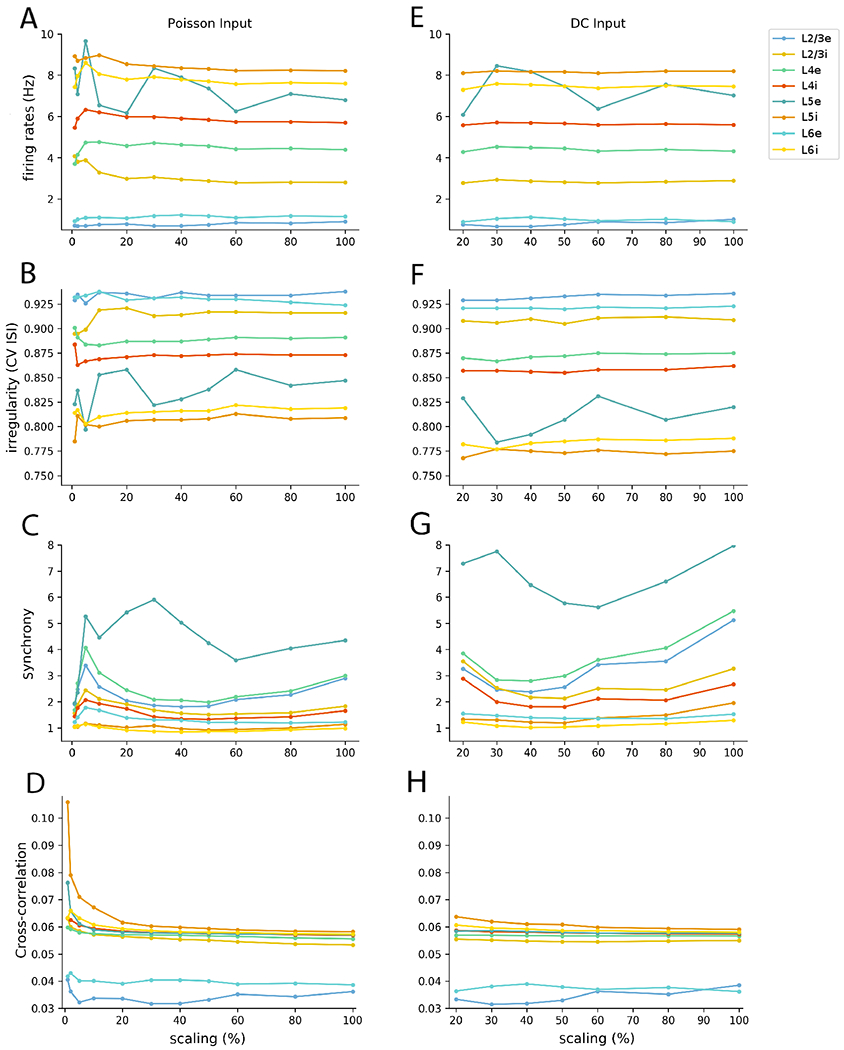
Mean population firing rate (A,E), irregularity (B,F), synchrony (C, G) and cross-correlation (D, H) of the 8 cell populations as a function of scaling for the NetPyNE reimplementation of the PDCM model, with Poisson (left) versus DC inputs (right). All results were calculated from 60 s simulations and approximately 1000 neurons except for cross-correlation where all 2-neurons combinations were considered
2.5. Replacing LIF with biophysically-detailed multicompartment neurons
As a proof-of-concept we modified the PDCM model by replacing the point neuron models with biophysically-detailed multicompartment neurons that included multiple ionic channels and synapses. We modified the original model through the following changes: 1. Replaced LIFs in all populations with a 6-compartment (soma, 2 apical dendrites, basal dendrite and axon) pyramidal neuron model with 9 conductance-based ionic channels (passive, Na+, 3 K+, 3 Ca2+, HCN) from Dura-Bernal et al. (2018). Neuron model parameters were imported from an existing JSON file. The required NMODL files were added to the repository and compiled. 2. Set temperature to 34°C, the temperature required for the cell model above to respond physiologically. 3. Added exponential (Exp2Syn) synapse models with with rise time constant, decay time and reversal potential (Erev) of 0.8 ms, 5.3 ms and 0 mV for excitatory synapses; and 0.6 ms, 8.5 ms and −75 mV for inhibitory synapses. These synapses were included in the connectivity rules. Weights were now all made positive, since inhibition was now mediated by a negative Erev. 4. Scaled all connection weights by 1e-6, given that weights here represent changes in conductance in NEURON μS units.
This version of the model is available as the “multicompartment” branch in the Github repository [github.com/suny-downstate-medical-center/PDCM_NetPyNE]
3. Results
3.1. Reproduction of Potjans-Diesmann (PDCM) model results
The NetPyNE implementation was able to reproduce the raster plot patterns as well as firing rates, irregularity and synchrony statistics for the balanced Poisson inputs condition (Figure 1; compare with Figure 6 of the original article (Potjans and Diesmann, 2014a)). The results are not identical due to different randomization of model drive and specific cell-to-cell wiring (see Discussion). Major characteristics of the original model that were reproduced including: 1. overall apparent asynchronous activity (but see details below); 2. lowest firing rates in L2/3e and L6e (~ 1 Hz) < L4e (~ 4 Hz) < L5e with the highest excitatory firing rate (~ 7 Hz); 3. irregularity ~ 0.8, lowest for L5i and L6i; 4. synchrony measure with L5e > L2/3e, L4e > L5i, L6i.
Figure 1:
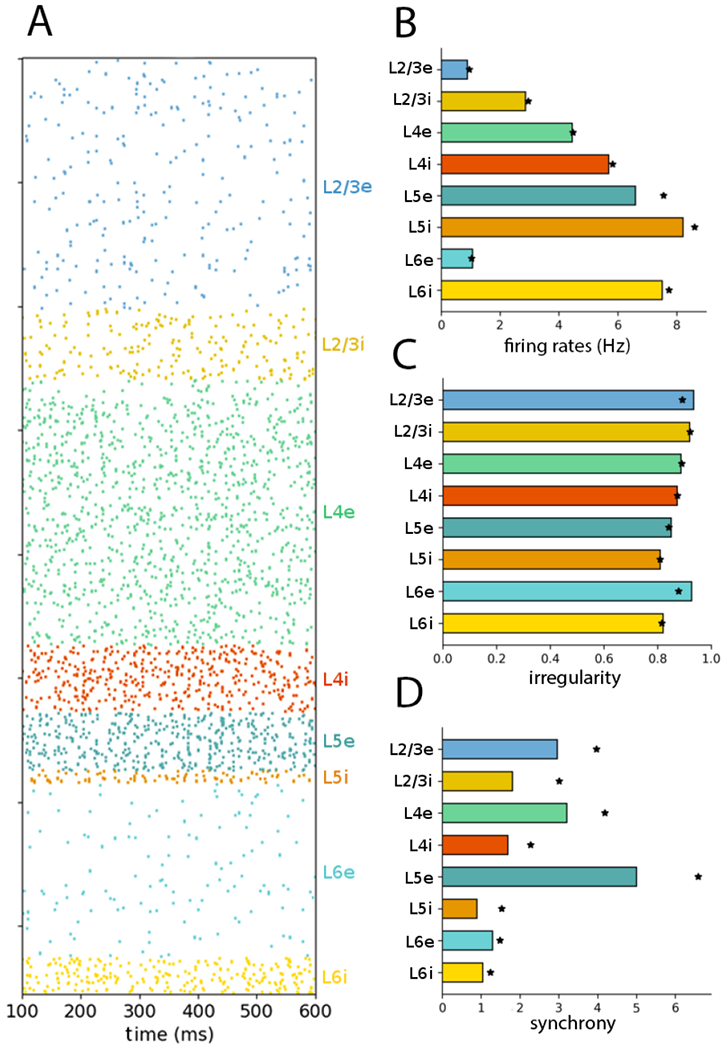
NetPyNE PDCM model with balanced Poisson inputs reproduces Fig. 6 of original article (Potjans and Diesmann, 2014a) (A) Raster plot showing activity of 1862 neurons for 500 ms. (B) Population mean firing rates over 60 s. (C) Population firing irregularity (CV ISI) over 60 s. (D) Population synchrony (normalized spike count variance over 5s). Statistics based on fixed sample of 1000 neurons/layer as in original model. Stars show statistics from Figure 6 of the original article.
A comparison of the mean population firing rates of the NetPyNE implementation with the original implementation (taken from Table 6 of the original article) is given in Table 2. To perform this comparison, we ran the NetPyNE simulations with different seeds for the random number generator. More specifically, we simulated the 100% scale network for 60 s with 10 different seeds, and calculated the mean and standard deviation across the neurons in all 10 simulations for each of the populations. We compared these results with the NEST results, which consisted of a single 60 s simulation with a fixed random number generator seed. The mean rates of the excitatory populations in the NEST implementation fall within 0.16 σ (0.16 of the standard deviation ranges) of their respective counterparts in the NetPyNE implementation. The relative deviations (|fNEST − fNetPyNE|/fNEST) is less than 11%. Considering the NEST subsampling of 1000 neurons per population, the standard normal random variables z (Z-scores) and p-values of the statistical comparison between the original model and the NetPyNE model firing rates were: L2/3e: 1.33, 0.184; L2/3i: 2.15, 0.016; L4e: 0.50, 0.615; L4i: 0.90, 0.179; L5e: 5.12, 3·10−7; L5i: 2.13, 0.017; L6e: 0.92, 0.367; and L6i: 0.75, 0.226.
Table 2:
Comparison of PDCM population-specific firing rates (Hz) for NEST and NetPyNE implementations.
| Platform | L2/3e | L2/3i | L4e | L4i | L5e | L5i> | L6e | L6i |
|---|---|---|---|---|---|---|---|---|
| NEST (1 trial) | 0.86 | - | 4.45 | - | 7.59 | - | 1.09 | - |
| NetPyNE (1 trial) | 0.90 | 2.80 | 4.39 | 5.70 | 6.79 | 8.21 | 1.14 | 7.60 |
| NetPyNE (10 trials) | 0.91 ± 1.08 | 2.80 ± 2.36 | 4.39 ± 3.94 | 5.70 ± 4.50 | 6.77 ± 5.04 | 8.21 ± 5.88 | 1.14 ± 1.85 | 7.60 ± 6.03 |
The synchrony metric depended on sampling, differing substantially when using all 77,169 neurons instead of subsampling (Fig. 2). Synchrony in L2/3e and L4e was now visible in the raster plot, and the synchrony values increased considerably for these populations compared to Fig. 1. Irregularity and mean firing rates were adequately captured with subsampling: the maximum variation (|fsub − fall|/fall) was less than 0.4%.
Figure 2:
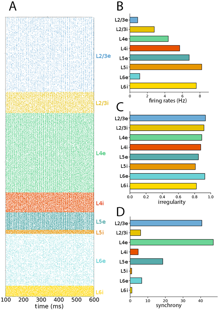
NetPyNE PDCM model with all 77,169 neurons included reveals synchrony is altered when subsampling is not used (compare to subsampled version in Fig. 1). (A) Raster plot with all neurons included shows synchronized activity in multiple populations. (B) Population mean firing rates; remain similar to the subsampled version. (C) Population firing irregularity (CV ISI); remains similar to the subsampled version; (D) Population synchrony values; differ compared to subsampled version.
We next tested the balanced DC input and unbalanced Poisson input protocols (compare Fig. 3 to panels A1, A2, B1 and B2 from Figure 7 in original publication (Potjans and Diesmann, 2014a)). As in the original model, replacing the balanced Poisson inputs with DC current did not affect the irregular firing displayed in the raster plot nor the population average firing rate properties. However, replacing them with unbalanced Poisson inputs resulted in loss of activity in L6e and modified the average firing rates across populations.
Figure 3:
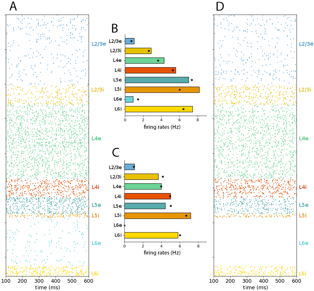
NetPyNE PDCM model with DC current and unbalanced Poisson input conditons reproduces Fig. 7 of original article (Potjans and Diesmann, 2014a): (A) Balanced DC inputs: raster plot (subsampled; only includes 1862 cells). (B) Balanced DC inputs: population mean firing rates over 60 s. (C) Unbalanced Poisson inputs: population mean firing rates over 1 s. (D) Unbalanced Poisson inputs: raster plot (subsampled; only shows 1862 cells). Statistics based on 1000 neurons per layer. Stars show statistics corresponding to Figure 7 of the original article.
3.2. Network scaling
Now that we have compared the full scale versions of the NetPyNE and NEST implementations with different sampling sizes, we will proceed to compare the scaled down NetPyNE implementations with the full scale NEST implementation.
Figures 4–6 show raster plots and statistics for scaled down NetPyNE versions of the PDCM model, with either Poisson or DC external inputs. As in the original article (Potjans and Diesmann, 2014a), raster plots show 1862 cells and the statistical measures were calculated using a fixed number of 8000 neurons. The raster plots exhibit similar firing patterns, and mean firing rate and irregularity per neuronal population as the full scale raster plot (Figure 1), both when using Poisson inputs (panels A-C of Figures 4, 5 and 6) and DC inputs (panels E-G of Figures 4 and 5). Although the raster plot appears to show all populations as asynchronous, the synchrony measure plot reveals high values for some populations (panels A and D of Figures 4, 5 and 6) and DC inputs (panels E and H of Figures 4 and 5). The raster plot and synchrony for the 10% scaling with DC external inputs case differed from the full scale results (Figure 1), as the raster plot exhibited a visually perceptible synchrony (Figure 6E), and the calculated synchrony value was considerably higher (Figure 6H).
Figure 4:
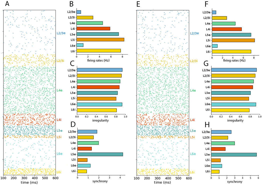
NetPyNE PDCM network rescaled to 50% of the number of neurons (A) Raster plot and (B–D) statistics for external Poisson input. (E) raster plot and (F–H) statistics for external DC current. The time interval and number of neurons sampled and plotted were chosen as in Figure 1.
Figure 6:
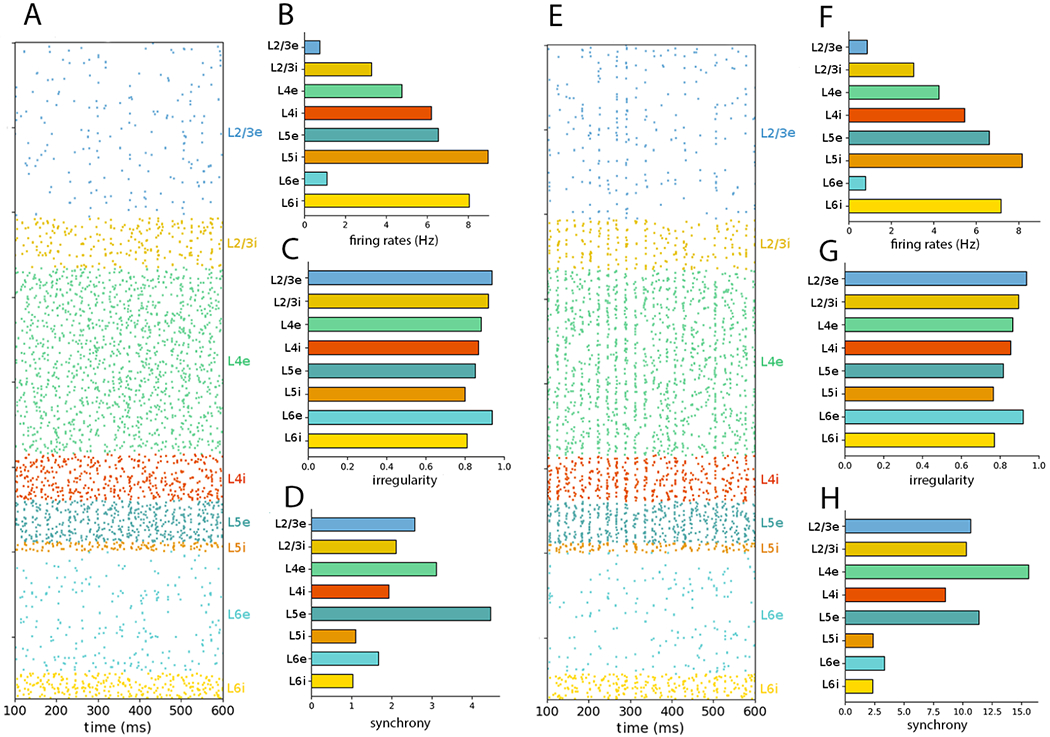
NetPyNE PDCM network rescaled to 10% of the number of neurons (A) Raster plot and (B–D) statistics for external Poisson input. (E) raster plot and (F–H) statistics for external DC current. The time interval and number of neurons sampled and plotted were chosen as in Figure 1.
Figure 5:
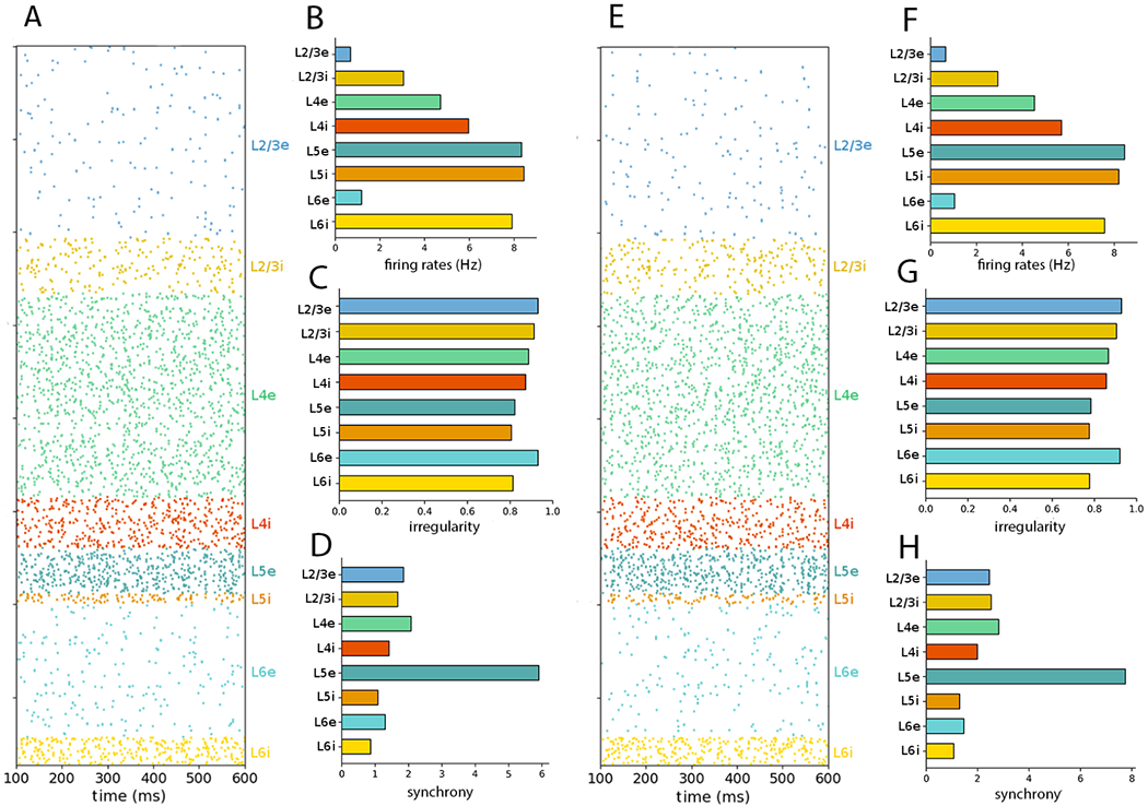
NetPyNE PDCM network rescaled to 30% of the number of neurons. (A) Raster plot and (B–D) statistics for external Poisson input. (E) raster plot and (F–H) statistics for external DC current. The time interval and number of neurons sampled and plotted were chosen as in Figure 1.
Note that the total number of neurons of scaled version may not exactly match that fraction of the total number of neurons (e.g. the 10% scale version has 7713, whereas the full-scale version has 77,169 cells), because scaling is performed for each population separately, resulting in the accumulation of small rounding errors.
To test whether neuron subsampling affects the results in the rescaled networks, in Figure 7 we evaluated the 30% rescaled network with no subsampling, i.e. including all 23,147 in the raster plot and statistics calculation (compare to Figure 5). Similarly to what was seen in the full scale network simulation (Figure 2), spike synchrony was visually perceptible in the raster plots and the population synchrony values were significantly altered.
Figure 7:
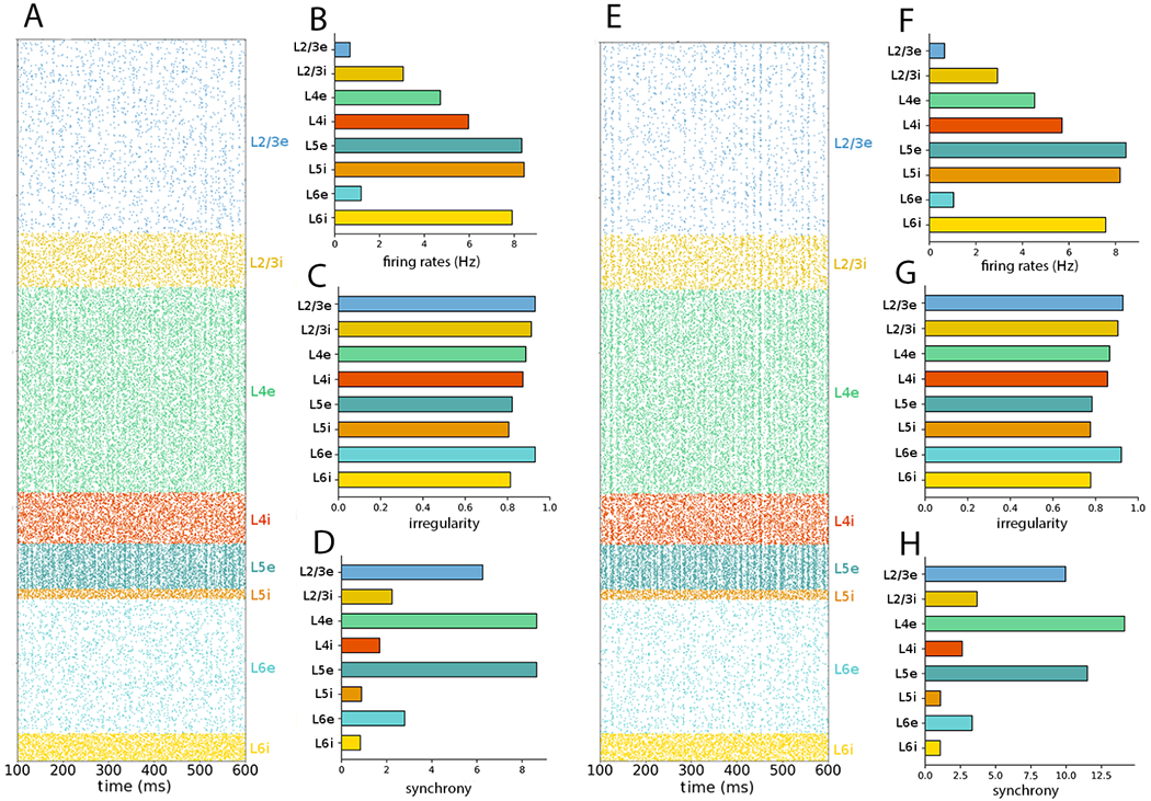
NetPyNE PDCM network rescaled to 30% of the number of neurons with no subsampling. (A) Raster plot and (B–D) statistics for external Poisson input. (E) Raster plot and (F–H) statistics for external DC current. Raster plots and statistics include all the neurons in the network.
Figure 8 summarizes the NetPyNE PDCM scaling results: model mean firing rate, irregularity, synchrony, and average cross-correlation for each cell population as a function of the degree of scaling and external input type. The complete dataset is available in Supplementary Tables S1 (mean firing rates, Poisson input), S2 (mean firing rate, DC input), S3 (irregularity, Poisson input), S4 (irregularity, DC input), S5 (synchrony, Poisson input), S6 (synchrony, DC input), S7 (average cross correlation, Poisson input), and S8 (average cross correlation, DC input). They allow a comparison of the different rescaled NetPyNE PDCM models and the original NEST implementation.
For both Poisson and DC external inputs, the mean population firing rates of all rescaled versions are close to the original results (Potjans and Diesmann, 2014a). For Poisson inputs, even extreme downscaling to 1% resulted in average firing rates consistent with the original NEST model (Supplementary Table S1). For DC inputs, downscaling the network below 10% resulted in no firing activity due to insufficient spiking input (i.e., an average neuron potential lower than the spiking threshold with a small variance results in almost nonexistent spike activity). Nevertheless, the average firing rates of the DC input models with downscaling above 10% also are consistent with the original article results (Supplementary Table S2). Overall, the highest relative deviation of the mean population firing rate between the rescaled NetPyNE and the original PD article (|fX%inNetPyNE − fNEST|/fNEST) data from Tables 2, S1, and S2.)
The mean population firing rates of the downscaled models presented overall small relative deviations with respect to the full-scale network results (Figure 8 and Tables S1 and S2). Relative deviation was calculated as (|fX% − f100%|/f100%). The populations with the largest relative deviations were L2/3e and L2/3i but even these generally exhibited maximum relative deviations under 30%. Networks with Poisson inputs tended to exhibit the largest relative deviations when downscaling below 10%, whereas networks with DC inputs started to display large relative deviations earlier on, when downscaling 40% and below.
The relative deviations of the irregularity measure across downscaled models compared to the full scale model ((|Ix% − I100%|/I100%)) were much smaller than that of the mean firing rate, with values around or below 1% (Figure 8 and Tables S3 and S4). The populations with the largest relative deviations for the measure were L5e and L5i.
Next, we evaluated the effect of downscaling on network synchrony. We first compared four different subsampling approaches to illustrate the effect of sample size in the synchrony calculation:
Sample a fixed percentage (8,000/77,169 = 10.37%) of neurons per population, totaling 8,000 neurons.
Sample 1,000 neurons per population, totaling 8,000 neurons (as in the original article).
Sample 2,000 neurons per population, totaling 16,000 neurons.
Not to sample and include all 77,169 neurons.
In contrast to irregularity, synchrony depends on the sampling strategy (see Table 3). However, it does not depend on the time window (5 s in Figures 1 and 2 and 60 s in Table 3 and Figure 8). The observed discrepancies in synchrony may be a consequence of sampling a different number of neurons or a different percentage of the population size (see the Discussion section). Interestingly, with the exception of L5i and L6i, synchrony appears to increase linearly with the number of sampled neurons from each population (Table 3). For comparison, we show in Figure 8 the synchrony of each population for the full-scale and downscaled NetPyNE implementations using the sampling strategy of the original article (1000 neurons per layer) (more details are given in Tables S5 and S6).
Finally, we evaluated the mean cross-correlation (defined in eqn. (10)) per layer as a second order statistic measure alternative to synchrony (Figure 8). The relative deviations of the mean cross-correlation across downscaled versions above 10% compared to full scale was much smaller than that of synchrony, with values around or below 12% for Poisson and 18% for DC external input (Figure 8 and Tables S7 and S8). However, for downscaling under 10%, the relative deviations increased and reached a maximum of 82% for L5i. The populations with the largest for cross-correlation relative deviations were L2/3e for scalings above 10% and L5 for scalings below 10%.
3.3. Additional model analysis facilitated by NetPyNE
Converting the PDCM model to the NetPyNE standardized specifications allows the user to readily make use of the tool’s many built-in analysis functions. These range from 2D visualization of the cell locations to different representations of network connectivity to spiking activity and information flow measures. Importantly, these are available to the user through simple high-level function calls, which can be customized to include a specific time range, frequency range, set of populations, and visualization options.
We illustrate the range of NetPyNE’s analysis capabilities using the PDCM model reimplementation in NetPyNE 9. All analyses were performed on the 10%-scaled version with 7,713 cells and over 30M synapses, simulated for 4 biological seconds. First, we visualized the network cell locations from the top-down (Figure 9A) and side (Figure 9B) views, which provided an intuitive representation of the cylindrical volume modeled, and the layer boundaries for each population. Next we plotted a stacked bar graph of convergence (Figure 9C), a measure of connectivity that provides at-a-glance information on the average number and distribution of presynaptic inputs from each population. We then analyzed the spectrotemporal properties of the network’s spiking activity through a Morlet wavelet-based spectrogram Büssow (2007) (Figure 9D); results depicted time-varying broad frequency peaks in the gamma range (40-80 Hz), consistent with the largely irregular and asynchronous network activity. Finally, we measured the spectral Granger causality Chicharro (2011) between L4e and L2/3e cells and found stronger information flow from L4e to L2/3i than vice-versa, particularly at gamma range frequencies, consistent with the canonical microcircuit (Douglas et al., 1989). Information flow analysis can reveal functional circuit pathways, including those involving inhibitory influences, that are not always reflected in the anatomical connectivity.
Figure 9:
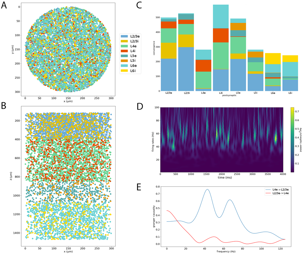
Analysis of model structure and simulation results facilitated by NetPyNE. (A) Top-down view (x-y plane) of network cell locations illustrates the diameter of the cylindrical volume modeled. (B) Side view (x-z plane) of network cell locations reveals cortical layer boundaries and populations per layer. Color indicates cell populations (see legend). (C) Stacked bar graph of the average connection convergence (number of presynaptic cells targeting each postsynaptic cell) for each population. (D) Spectrogram of average firing rate across all cells illustrating time-varying peaks in the gamma oscillation range. (E) Spectral Granger causality between L4e and L2/3i populations indicates stronger information flow from L4e to L2/3i than vice-versa.
3.4. Network with biophysically-detailed multicompartment neurons
An additional advantage of the NetPyNE implementation of the PDCM model is the ability to easily modify the model to include more biophysically-detailed features that could, for example, provide insights into dendritic function or extracellular field potentials. As a proof-of-concept we implemented a version of the PDCM model with multicompartment neurons with multiple conductance-based ion channels and synapses (Fig. 10A). The implementation of this model required only minimal changes in the source code (see Methods Section 2.5 for details), demonstrating the usefulness of NetPyNE as a high-level language to specify and modify network models.
Figure 10:
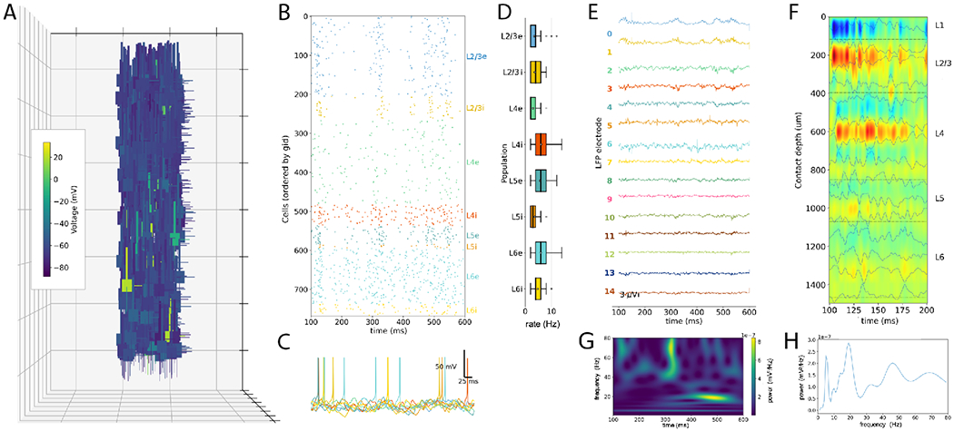
NetPyNE-based PDCM model with biophysically-detailed multicompartment neurons. (A) 3D representation of all network neurons with color indicating membrane voltage at t=150ms (each grid square is 250 μm). (B) Spike raster plot. (C) Example voltage traces for each population. (D) Firing rate statistics. (E) Local field potential (LFP) signal recorded from 15 simulated electrodes at different depths (100 μm interval) (F) Current source density (CSD) profiles calculated from LFP with color indicating current strength and direction (sinks=red; sources=blue). (G) LFP power spectrogram for electrode at 300 μm depth. (H) LFP power spectral density for electrode at 300 μm depth.
We simulated the new biophysically-detailed PDCM model (at 1% scale for 600 ms) and obtained physiological-like activity in all populations (Fig. 10B). It is out of the scope of this paper to tune the new version to reproduce the original model statistics. However, the preliminary firing rate statistics, without additional parameter tuning, are consistent with the original (Fig. 10D). This implementation also allowed to simulate previously unavailable biological measures, including membrane voltage at different neuron compartments (Figs. 10A,C), ionic and synaptic currents, local field potential and current source density at different depths (Figs. 10E,F). LFP spectral analysis (Fig. 10E,F) revealed time-varying oscillations in the beta and gamma range consistent with cortical dynamics (Buzsáki and Draguhn, 2004).
4. Discussion
We reimplemented the PDCM model using the NetPyNE tool, a high-level interface to the NEURON simulator. The new model version reproduced the overall network dynamics of the original PDCM model, evaluated through population-specific average firing rates, irregularity and synchrony measures. The NetPyNE version allowed simplified scaling of network size, while preserving the network statistics for most conditions. This feature can be used to study the effect of scaling on network dynamics. For example, under certain conditions, network synchrony increased for smaller networks, as explained in section 4.5 below.
4.1. Advantages of NetPyNE implementation
Source code for the NetPyNE implementation is available in GitHub:github.com/suny-downstate-medical-center/PDCM_NetPyNE and on ModelDB: modeldb.yale.edu/266872 (password: PD_in_NetPyNE). NetPyNE provides a clear separation of model specifications and the underlying low-level implementation, and facilitates extension of the model. This was demonstrated by modifying the PDCM model to include more biophysically-realistic multicompartment neuron models (Figure 10). This version, which produced similar dynamics, enabled recording membrane voltage and ionic currents, and simulating local field potentials (LFPs) and current source density (CSD) analysis, permitting more direct comparison to experimental data.
The LFPy tool hybrid scheme Hagen et al. (2016a) also offers a method to calculate LFP signals in point-neuron networks. To do this it generates a network of simplified multicompartment neurons with a passive membrane model that preserves the original network features. This provides an efficient method to predict extracellular potentials in large point-neuron networks, but requires generating and running a separate model. The NetPyNE implementation provides a single network model, with fully customizable neuron biophysics and morphologies, which can be simulated to obtain neural data at multiple scales: from membrane voltage and currents to spiking activity to LFPs. The LFPy hybrid scheme likely provides a faster method to obtain LFP estimates in point neuron networks.
The NetPyNE implementation of the original model also enabled employing NetPyNEs analysis capabilities to gain further insights into the model. This was illustrated by visualizing the network’s topology and connectivity, plotting the average firing rate spectrogram and calculating the spectral Granger causality (a measure of information flow) between two model populations (Figure 9).
NetPyNE provides integrated analysis and plotting functions that avoid the need to read and manipulate the output data using a separate tool. An alternative approach is to separate modeling and analysis code to avoid maintaining separate implementations of core analysis functions. For this purpose, NetPyNE simulation outputs can also be saved to common formats and analyzed by other tool such as Elephant (Electrophysiology Analysis Toolkit).
4.2. Reproduction of original results
We were able to reproduce all the network statistics (mean firing rate, irregularity and synchrony) for the three types of external inputs: balanced Poisson, DC current, and unbalanced Poisson – compare Figure 1 with Figure 6 of the original article (Potjans and Diesmann, 2014a)), and Figure 3 with Figure 7 of the original article. The mean rates of the excitatory neurons of the NEST implementation fall within 0.16 σ of the NetPyNE results. The low p-value obtained for layer L5e is probably due to the high variability of the average firing rates, a feature described in Figure 8-C of the original article Potjans and Diesmann (2014a). Notably, in the unbalanced Poisson input condition, we can observe the lack of activity in L6e and the firing rate changes in other populations, both present in the original study.
4.3. Preserved statistics in rescaled networks
The scaling method works by keeping the random inputs unchanged on average (van Albada et al., 2015) and fixing the proportion between the firing threshold and the square root of the number of connections (van Vreeswijk and Sompolinsky, 1998) (see parameters in Table 1). This method managed to approximately preserve the mean firing rate and irregularity for all populations across all scaling percentages, ranging from 90% to 1% (Figure 8 and Tables S1 to S4). The synchrony measure was similarly preserved for the Poisson external input condition (Table S5), but not for the DC input condition, as discussed in section 4.5.
The second order measures, synchrony and cross-correlation, showed an increased relative deviation from the full scale network when downscaling below 10%. It is important to point out that any scaling method has limitations due to mathematical constraints. The downscaling ceases to maintain the second order statistics when the condition w << (θ − Vreset) is not satisfied (see Section 4.4). This may be one of the reasons for the observed increase in relative deviations below 10% downscaling.
Downscaled models are extremely useful for exploratory work and educational purposes because they reduce the required computational resources. For example, they can be used to study aspects requiring long simulation times, such as the learning window of spike-time-dependent plasticity (STDP) (Clopath et al., 2010), or requiring detailed multi-compartment neurons, such as the effect of adrenergic neuromodulation of dendritic excitability on network activity (Dura-Bernal et al., 2019a; Labarrera et al., 2018).
4.4. Mathematical explanation and limitations of the scaling method
The scaling method implemented in our model was based on previous theoretical work: van Vreeswijk and Sompolinsky (1998) and van Albada et al. (2015). The technique employed two independent parameters: one of them maintained the cross correlation and number of neurons but changed the number of connections, and so, the probability of connections; the other one decreased the network size without guaranteeing a preservation of second order statistics, including cross correlation.
The parameters in these studies related to internal connections (μint, σint), such as the number of incoming synapses per neuron and the internal synaptic weights were modified appropriately. However, none of the parameters related to external input (external drive) were adapted. Instead, the external drive (μext, σext) compensated for changes in μ and σ. According to eqn. 16 from van Albada et al. (2015), this imposed a limit to the downscaling factor:
| (12) |
The scaling method available as source code from the Open Source Brain (OSB) platform (Potjans and Diesmann, 2014b) appears to be derived from the two-independent-parameter approach, although its provenance is not fully documented. This OSB implementation allowed for different ways to rescale the network, some of which did not preserve network statistics.
Following van Vreeswijk and Sompolinsky (1998), we preserved network statistics by scaling both internal connections and external inputs, combining the two parameters into a single k parameter. This preserved the network second order statistics ( and ). In the original scaling method, only is downscaled and so eqn. 12 imposes a limitation on the scaling factor. However, in our approach, both and are downscaled proportionally, so the quotient of eqn 12 remains constant and this limitation does not apply. Note that our scaling factor k is different from the k2015 (eqn. 12) used in van Albada et al. (2015).
More formally (Romaro et al., 2020), given a sparsely connected random network model where the input u(t) to a neuron is given by
| (13) |
where η(t) is an uncorrelated Gaussian white noise with zero mean, the working points of the neuron population can be characterized by its mean μ and standard deviation σ. In order to preserve all other network features, including firing rate and time constants, let us write:
| (14) |
| (15) |
where and are the average number of internal and external connections that a neuron receive and the are the respective average synaptic weights. The transformation N′ = kN, I′ = kI, preserves σ – first 3 steps of scaling – but reduces μ by . The introduction of a DC input of – fourth step of scaling – cancels this reduction. For more details, see Romaro et al. (2020).
This scaling method presented limitations both in terms of the working point and the preserving statistics, especially for small values of k, when the synaptic weights no longer satisfied the condition: w << (θ − Vreset) (synaptic weight much smaller than the amplitude from voltage reset to firing threshold).
Overall, our scaling implementation was simplified and adapted in order to guarantee the conservation of the first μ and second σ order statistics of network activity for all possible scalings while making it easy to implement in NetPyNE/NEURON. It is dependent on a single scaling factor, k, in the interval (0, ∞), presented in Table 1, which is used to adapt the number of network neurons, connections and external inputs as well as the synaptic weights, while keeping the matrix of connection probabilities and the proportions of cells per population fixed.
The scaling method does not change any other network parameters, including τm, τs, τref, R, Vreset, the relative inhibitory synaptic strength g, excitatory or inhibitory synaptic transmission delays de and di, and firing threshold θ.
4.5. Multiple factors affect synchrony
The synchrony measure was dependent on the number of neurons used in its calculation, in general with a higher number of neurons resulting in higher synchrony values. Because of the different sampling strategies, comparing synchrony across populations and network models should be done with caution. For example, when we compared synchrony across populations, sampling a fixed percentage of neurons per population (Table 3 top row), the two largest populations, namely L2/3e and L4e, exhibited the highest synchrony values. On the other hand, when we sampled a fixed number of neurons from each population, 1000 as in the original model (Table 3 middle row) or 2000 (Table 3 bottom row), the highest synchrony was displayed by population L5e. The strategy of sampling a fixed number of neurons per population also may lead to scaling distortions because a given fixed number corresponds to different percentages of the cell populations at each scaling degree. For example, in the full scale version 1000 corresponds to almost 100% of L5i neurons but to less than 5% of L2/3e neurons. When downscaling was too great (< 20%), there were not enough neurons in a population to do the full subsampling and include in the calculation.
Choosing the number of neurons to estimate synchrony as a percentage also influenced the synchrony measure. For example, the raster plot and synchrony for the Poisson-driven full-scale network indicated, both visually and numerically, a high degree of synchrony when all neurons (~80,000) were sampled (Figure 2), but a low degree of synchrony when only 2.3% of the neurons were sampled (Figure 1). The same phenomenon was observed in the rescaled implementations. For example, the 30% rescaled network displayed high synchrony when all neurons (~23,000) were sampled (Figure 7), and low synchrony when a small subset of neurons (~2000) was sampled (Figure 5). This leads us to conclude that the apparent asynchrony in the PDCM model is possibly a consequence of subsampling. The influence of subsampling on synchrony has been previously studied (Harris and Thiele, 2011; Tetzlaff et al., 2012; Hagen et al., 2016b), and synchrony in the PDCM network has been previously described (see Figure 8C in Hagen et al. (2016b)).
In general, synchrony tended to decrease with the degree of downscaling (see plots at the bottom of Figure 8). This was due to the increase in injected current that we provided to compensate for the decreased number of connections (see Section 2.3). This effect occurred up to a downscaling level that depended on the population and external input type (between 40% and 60%). Downscaling past this point, we reached a situation in which the number of neurons was not sufficient to allow reliable synchrony calculation. For example, when we downscaled the networks to 10% of the original size, we had to replace 99% of the connections with DC inputs, and this resulted in large increases in synchrony (Figure 8, bottom plots).
Synchrony was also dependent on the population average firing rate. The synchrony measure used (see Methods) changed with the heterogeneity of firing within the cell population (Pinsky and Rinzel, 1995), which for equal population sizes and fixed bin size is higher for cells with higher firing rates. This dependence may be a possible explanation for the high synchrony of L5e neurons (Figure 8 bottom plots; see also Tables S5 and S6).
Synchrony was generally higher under the DC input condition than the Poisson input condition (Figure 8 bottom plots; see also Tables S5 and S6). We hypothesize this was due to the two sources of randomization present in the Poisson-driven network: the Poisson inputs and the random pattern of connection. The third source of randomness, the initial values of the membrane potential of the neurons, should not be a cause for the high synchrony found, given the omission of the initial 100 ms transient period on the estimation of the measure. In the DC condition we removed the Poisson inputs, thus increasing the network synchrony. For very high downscaling, e.g. 10%, synchrony becomes visually perceptible in the raster plot for DC inputs but not in the one for Poisson inputs (compare Figures 6H and 6D). This effect is not seen for intermediate downscaling levels, cf. Figures 4D,H (50% downscaling) and 5D,H (30% downscaling) because the fraction of sampled cells is not high enough.
Since multiple factors affect synchrony, we calculated the mean cross-correlation as an alternative measure based on second order statistics. This metric was preserved for models downscaled to factors over 20%, and generally presented lower relative deviations than the synchrony measure.
The scaling method used here has the theoretical property of not adding synchrony or regularity to asynchronous irregular networks (van Vreeswijk and Sompolinsky, 1998; van Albada et al., 2015). In our study, we found that irregularity, synchrony and mean cross-correlation (second order statistics) did not appear to be affected by scaling down to 1% for Poisson inputs and to 20% for DC inputs, and the mean firing rates (first order statistic) of the original article (Potjans and Diesmann, 2014a) were within 0.16 standard deviations of our results.
Supplementary Material
Acknowledgments
This work was produced as part of the activities of NIH U24EB028998, R01EB022903, U01EB017695, NYS SCIRB DOH01-C32250GG-3450000, NSF 1904444; and FAPESP (S. Paulo Research Foundation) Research, Disseminations and Innovation Center for Neuromathematics 2013/07699-0, 2015/50122-0, 2018/20277-0. C.R. (grant number 88882.378774/2019-01) and F.A.N/ (grant number 88882.377124/2019-01) are recipients of PhD scholarships from the Brazilian Coordenao de Aperfeioamento de Pessoal de Nvel Superior (CAPES). A.C.R. is partially supported by a CNPq fellowship (grant 306251/2014-0).
References
- Beul SF and Hilgetag CC (2015). Towards a canonical agranular cortical microcircuit. Frontiers in Neuroanatomy, 8:165. [DOI] [PMC free article] [PubMed] [Google Scholar]
- Bezaire MJ, Raikov I, Burk K, Vyas D, and Soltesz I (2016). Interneuronal mechanisms of hippocampal theta oscillation in a full-scale model of the rodent ca1 circuit. eLife, 5:e18566. [DOI] [PMC free article] [PubMed] [Google Scholar]
- Binzegger T, Douglas RJ, and Martin KA (2004). A quantitative map of the circuit of cat primary visual cortex. Journal of Neuroscience, 24(39):8441–8453. [DOI] [PMC free article] [PubMed] [Google Scholar]
- Bos H, Diesmann M, and Helias M (2016). Identifying anatomical origins of coexisting oscillations in the cortical microcircuit. PLoS Computational Biology, 12(10):e1005132. [DOI] [PMC free article] [PubMed] [Google Scholar]
- Brunel N (2000). Dynamics of sparsely connected networks of excitatory and inhibitory spiking neurons. Journal of Computational Neuroscience, 8(3):183–208. [DOI] [PubMed] [Google Scholar]
- Büssow R (2007). An algorithm for the continuous morlet wavelet transform. Mechanical Systems and Signal Processing, 21(8):2970–2979. [Google Scholar]
- Buzsáki G and Draguhn A (2004). Neuronal oscillations in cortical networks. science, 304(5679):1926–1929. [DOI] [PubMed] [Google Scholar]
- Cain N, Iyer R, Koch C, and Mihalas S (2016). The computational properties of a simplified cortical column model. PLoS Computational Biology, 12(9):e1005045. [DOI] [PMC free article] [PubMed] [Google Scholar]
- Carnevale NT and Hines ML (2006). The NEURON Book. Cambridge University Press. [Google Scholar]
- Chicharro D (2011). On the spectral formulation of granger causality. Biological cybernetics, 105(5):331–347. [DOI] [PubMed] [Google Scholar]
- Clopath C, BUsing L, Vasilaki E, and Gerstner W (2010). Connectivity reflects coding: a model of voltage-based stdp with homeostasis. Nature neuroscience, 13(3):344. [DOI] [PubMed] [Google Scholar]
- de Kock CP and Sakmann B (2009). Spiking in primary somatosensory cortex during natural whisking in awake head-restrained rats is cell-type specific. Proceedings of the National Academy of Sciences (USA), 106(38):16446–16450. [DOI] [PMC free article] [PubMed] [Google Scholar]
- Dean DC, Planalp E, Wooten W, Schmidt C, Kecskemeti S, Frye C, Schmidt N, Goldsmith H, Alexander AL, and Davidson RJ (2018). Investigation of brain structure in the 1-month infant. Brain Structure and Function, 223(4):1953–1970. [DOI] [PMC free article] [PubMed] [Google Scholar]
- Douglas RJ, Martin KA, and Whitteridge D (1989). A canonical microcircuit for neocortex. Neural computation, 1(4):480–488. [Google Scholar]
- Dura-Bernal S, Neymotin S, Suter B, GMG S, and Lytton W (2018). Multiscale dynamics and information flow in a data-driven model of the primary motor cortex microcircuit. bioRxiv, (201707). [Google Scholar]
- Dura-Bernal S, Neymotin SA, Suter BA, Kelley C, Tekin R, Shepherd GM, and Lytton WW (2019a). Cross-frequency coupling and information flow in a multiscale model of m1 microcircuits. In Society for Neuroscience (SFN’19). [Google Scholar]
- Dura-Bernal S, Suter BA, Gleeson P, Cantarelli M, Quintana A, Rodriguez F, Kedziora DJ, Chadderdon GL, Kerr CC, Neymotin SA, McDougal RA, Hines M, Shepherd GM, and Lytton WW (2019b). Netpyne, a tool for data-driven multiscale modeling of brain circuits. eLife, 8:e44494. [DOI] [PMC free article] [PubMed] [Google Scholar]
- Gewaltig M-O and Diesmann M (2007). NEST (neural simulation tool). Scholarpedia, 2(4):1430. [Google Scholar]
- Hagen E, Dahmen D, Stavrinou ML, Lindén H, Tetzlaff T, van Albada SJ, GrUn S, Diesmann M, and Einevoll GT (2016a). Hybrid scheme for modeling local field potentials from point-neuron networks. Cerebral Cortex. [DOI] [PMC free article] [PubMed] [Google Scholar]
- Hagen E, Dahmen D, Stavrinou ML, Lindén H, Tetzlaff T, van Albada SJ, Griin S, Diesmann M, and Einevoll GT (2016b). Hybrid scheme for modeling local field potentials from point-neuron networks. Cerebral cortex, pages 1–36. [DOI] [PMC free article] [PubMed] [Google Scholar]
- Harris KD and Thiele A (2011). Cortical state and attention. Nature reviews neuroscience, 12(9):509–523. [DOI] [PMC free article] [PubMed] [Google Scholar]
- Hines ML, Morse T, Migliore M, Carnevale NT, and Shepherd GM (2004). Modeldb: a database to support computational neuroscience. Journal of Computational Neuroscience, 17(1):7–11. [DOI] [PMC free article] [PubMed] [Google Scholar]
- Labarrera C, Deitcher Y, Dudai A, Weiner B, Amichai AK, Zylbermann N, and London M (2018). Adrenergic modulation regulates the dendritic excitability of layer 5 pyramidal neurons in vivo. Cell reports, 23(4):1034–1044. [DOI] [PubMed] [Google Scholar]
- Lapicque L (1907). Recherches quantitatives sur l’excitation electrique des nerfs traitee comme une polarization. Journal de Physiologie et de Pathologie Generale, 9:620–635. [Google Scholar]
- Lee JH, Koch C, and Mihalas S (2017). A computational analysis of the function of three inhibitory cell types in contextual visual processing. Frontiers in Computational Neuroscience, 11:28. [DOI] [PMC free article] [PubMed] [Google Scholar]
- Lytton WW, Seidenstein AH, Dura-Bernal S, McDougal RA, Schiirmann F, and Hines ML (2016). Simulation neurotechnologies for advancing brain research: parallelizing large networks in neuron. Neural Computation, 28(10):2063–2090. [DOI] [PMC free article] [PubMed] [Google Scholar]
- McDougal RA, Hines ML, and Lytton WW (2013). Reaction-diffusion in the neuron simulator. Frontiers in Neuroinformatics, 7:28. [DOI] [PMC free article] [PubMed] [Google Scholar]
- Newton AJH, McDougal RA, Hines ML, and Lytton WW (2018). Using neuron for reaction-diffusion modeling of extracellular dynamics. Frontiers in Neuroinformatics, 12:41. [DOI] [PMC free article] [PubMed] [Google Scholar]
- Neymotin SA, Dura-Bernal S, Lakatos P, Sanger TD, and Lytton W (2016). Multitarget multiscale simulation for pharmacological treatment of dystonia in motor cortex. Frontiers in Pharmacology, 7(157). [DOI] [PMC free article] [PubMed] [Google Scholar]
- Pinsky PF and Rinzel J (1995). Synchrony measures for biological neural networks. Biological cybernetics, 73(2):129–137. [DOI] [PubMed] [Google Scholar]
- Potjans TC and Diesmann M (2014a). The cell-type specific cortical microcircuit: relating structure and activity in a full-scale spiking network model. Cerebral cortex, 24(3):785–806. [DOI] [PMC free article] [PubMed] [Google Scholar]
- Potjans TC and Diesmann M (2014b). Spiking cortical network model potjans and diesmann (github commit hash d8d8a55): https://github.com/opensourcebrain/potjansdiesmann2014/tree/d8d8a55e0a0c9cab2de77aaf3a38d3afd32’
- Ranjan R, Khazen G, Gambazzi L, Ramaswamy S, Hill SL, Schürmann F, and Markram H (2011). Channelpedia: an integrative and interactive database for ion channels. Frontiers in Neuroinformatics, 5:36. [DOI] [PMC free article] [PubMed] [Google Scholar]
- Romaro C, Roque AC, and Piqueira JRC (2020). Boundary solution based on rescaling method: recoup the first and second-order statistics of neuron network dynamics. arXiv preprint arXiv:2002.02381. [Google Scholar]
- Sakata S and Harris KD (2009). Laminar structure of spontaneous and sensory-evoked population activity in auditory cortex. Neuron, 64(3):404–418. [DOI] [PMC free article] [PubMed] [Google Scholar]
- Schmidt M, Bakker R, Hilgetag CC, Diesmann M, and van Albada SJ (2018). Multi-scale account of the network structure of macaque visual cortex. Brain Structure and Function, 223(3):1409–1435. [DOI] [PMC free article] [PubMed] [Google Scholar]
- Schuecker J, Schmidt M, van Albada SJ, Diesmann M, and Helias M (2017). Fundamental activity constraints lead to specific interpretations of the connectome. PLoS Computational Biology, 13(2):e1005179. [DOI] [PMC free article] [PubMed] [Google Scholar]
- Schwalger T, Deger M, and Gerstner W (2017). Towards a theory of cortical columns: From spiking neurons to interacting neural populations of finite size. PLoS Computational Biology, 13(4):e1005507. [DOI] [PMC free article] [PubMed] [Google Scholar]
- Shimoura R, Kamiji N, Pena R, Lima Cordeiro V, Celis C, Romaro C, and Roque AC (2018). [re] the cell-type specific cortical microcircuit: relating structure and activity in a full-scale spiking network model. ReScience, 4. [DOI] [PMC free article] [PubMed] [Google Scholar]
- Sivagnanam S, Majumdar A, Yoshimoto K, Astakhov V, Bandrowski A, Martone ME, and Carnevale NT (2013). Introducing the neuroscience gateway. In IWSG. [DOI] [PMC free article] [PubMed] [Google Scholar]
- Swadlow HA (1989). Efferent neurons and suspected interneurons in s-1 vibrissa cortex of the awake rabbit: receptive fields and axonal properties. Journal of Neurophysiology, 62(1):288–308. [DOI] [PubMed] [Google Scholar]
- Tetzlaff T, Helias M, Einevoll GT, and Diesmann M (2012). Decorrelation of neural-network activity by inhibitory feedback. PLoS Comput Biol, 8(8):e1002596. [DOI] [PMC free article] [PubMed] [Google Scholar]
- Thomson AM, West DC, Wang Y, and Bannister AP (2002). Synaptic connections and small circuits involving excitatory and inhibitory neurons in layers 2–5 of adult rat and cat neocortex: triple intracellular recordings and biocytin labelling in vitro. Cerebral Cortex, 12(9):936–953. [DOI] [PubMed] [Google Scholar]
- Towns J, Cockerill T, Dahan M, Foster I, Gaither K, Grimshaw A, Hazlewood V, Lathrop S, Lifka D, Peterson GD, et al. (2014). Xsede: accelerating scientific discovery. Computing in Science & Engineering, 16(5):62–74. [Google Scholar]
- van Albada SJ, Helias M, and Diesmann M (2015). Scalability of asynchronous networks is limited by one-to-one mapping between effective connectivity and correlations. PLoS Computational Biology, 11(9):e1004490. [DOI] [PMC free article] [PubMed] [Google Scholar]
- van Vreeswijk C and Sompolinsky H (1998). Chaotic balanced state in a model of cortical circuits. Neural Computation, 10(6):1321–1371. [DOI] [PubMed] [Google Scholar]
- Wagatsuma N, Potjans TC, Diesmann M, Sakai K, and Fukai T (2013). Spatial and feature-based attention in a layered cortical microcircuit model. PloS One, 8(12):e80788. [DOI] [PMC free article] [PubMed] [Google Scholar]
- West DC, Mercer A, Kirchhecker S, Morris OT, and Thomson AM (2005). Layer 6 cortico-thalamic pyramidal cells preferentially innervate interneurons and generate facilitating epsps. Cerebral Cortex, 16(2):200–211. [DOI] [PubMed] [Google Scholar]
Associated Data
This section collects any data citations, data availability statements, or supplementary materials included in this article.


