Chromatin and transcription factor profiling in rare stem cell populations using CUT&Tag

Summary

Muscle stem cells (MuSCs) are a rare stem cell population that provides myofibers with a remarkable capacity to regenerate after tissue injury. Here, we have adapted the Cleavage Under Target and Tagmentation technology to the mapping of the chromatin landscape and transcription factor binding in 50,000 activated MuSCs isolated from injured mouse hindlimb muscles. We have applied this same approach to human CD34⁺ hematopoietic stem and progenitor cells. This protocol could be adapted to any rare stem cell population.

For complete details on the use and execution of this protocol, please refer to Robinson et al. (2021).

Graphical abstract

Highlights

• •Isolation of muscle stem cells from cardiotoxin-injured tissue
• •CUT&Tag-based mapping of epigenetic landscape and transcription factor enrichment
• •Adaptation of a synthetic spike-in DNA for effective normalization across samples
• •Pipeline for efficient analysis of CUT&Tag sequencing data hosted on Git-hub

Muscle stem cells (MuSCs) are a rare stem cell population that provides myofibers with a remarkable capacity to regenerate after tissue injury. Here, we have adapted the Cleavage Under Target and Tagmentation technology to the mapping of the chromatin landscape and transcription factor binding in 50,000 activated MuSCs isolated from injured mouse hindlimb muscles. We have applied this same approach to human CD34⁺ hematopoietic stem and progenitor cells. This protocol could be adapted to any rare stem cell population.

Before you begin

Adult tissue-resident stem cells are rare cell populations that maintain tissue homeostasis and are indispensable for growth and regeneration throughout life. In the case of skeletal muscle, myofiber damage is efficiently repaired through the activity of Muscle Stem Cells (MuSCs). However, harnessing the regenerative capacity of MuSCs therapeutically has been limited by our inability to fully characterize these rare stem cells. Thus, it is important to develop technologies that allow for the characterization of MuSCs without ex vivo expansion.

The epigenetic state of a cell is an important characteristic that defines the genes that are expressed. Epigenetic landscapes of MuSCs have been examined using formaldehyde cross-linking based ChIP-Seq protocols in MuSCs expanded ex vivo (Blum et al., 2012; Judson et al., 2018; Mousavi et al., 2012). A disadvantage of this approach is the large number of cells required to complete the protocol due to the inherent background noise associated with the technology. The ChIP-Seq approach also suffers from the appearance of false-positive identification of histone mark enrichment due to cross-linking of marked and unmarked regions of the genome. At the same time, false-negative results can be observed if the epitope of the antibody is masked by the presence of “reader” proteins as they become crosslinked to chromatin. The development of Native ChIP protocols mitigated the problem of false negatives (Benyoucef et al., 2016; Brand et al., 2008; Faralli et al., 2016; Grzybowski et al., 2019; O'Neill and Turner, 2003), but continued to require large number of cells to obtain a good signal above the background noise. To overcome the need for large number of cells, the Henikoff group recently described the Cleavage Under Target and Tagmentation (CUT&Tag) technology that uses a Tn5 transposase fused to Protein A (pA-Tn5) to tagment, antibody-bound regions of the genome in native (non cross-linked) conditions (Kaya-Okur et al., 2019). We have recently adapted this technology to examine the function of NELF in MuSC populations (Robinson et al., 2021). Furthermore, we have used it with a wide range of antibodies for both histones and transcription factors in either MuSCs or human CD34⁺ hematopoietic stem progenitor cells. Thus, this approach should be widely applicable across different cell-types using a broad range of antibodies.

Purification of the pA-Tn5 enzyme

Timing:7 days

This section details the preparation of the Protein A-Transposase fusion protein (pA-Tn5) required for introducing tags within the genome (Kaya-Okur et al., 2019; Picelli et al., 2014). Typically, it takes 7 days to prepare the enzyme. While this step is labor intensive, the enzyme is stable and can provide enough material for hundreds of experiments. Alternatively, pA-Tn5 can be purchased from commercial vendors. Purification of pA-Tn5 from bacterial extracts is detailed below.

• 1.
  Transformation of 3XFlag-pA-Tn5-Fl (Addgene #124601) into T7 Express lysY/Iq E. coli

  • a.
    Thaw a frozen aliquot of T7 Express lysY/Iq competent E. coli cells (NEB) on ice for 10 min.
  • b.
    Add 1–5 μL of the plasmid (contains 100 ng of plasmid DNA) to the cell mixture. Carefully flick the microcentrifuge tube 4–5 times to mix cells and DNA. Do not vortex.
  • c.
    Place the mixture on ice for 30 min.
  • d.
    Heat shock at 42°C for 10 s.
  • e.
    Place on ice for 5 min.
  • f.
    Pipette 950 μL of room temperature SOC media into the mixture.
  • g.
    Place at 37°C shaker (250 rpm) for 60 min.
  • h.
    Simulatenously, warm an agar selection plate containing ampicillin at 37°C.
  • i.
    After 60 min, mix the cells thoroughly by flicking and inverting the microcentrifuge tube.
  • j.
    Spread 50 μL of the mixture onto the selection agar plate containing ampicillin and incubate overnight at 37°C.
• 2.
  Expression of pA-Tn5 Transposase (protocol for 1 L culture, can be scaled accordingly)

  • a.
    Inoculate a single colony into 20 mL of LB Broth (Miller) containing 100 μg/mL ampicillin (or carbenicillin) and grow at 37°C for 6 h in an orbital shaker.
  • b.
    Use this 20 mL starter culture to inoculate 1 L of pre-warmed LB Broth. Distribute 200 mL of inoculated LB Broth across five 1-L Erlenmeyer flasks. Grow at 37°C and monitor the culture until OD₆₀₀ reaches ∼0.6 (about 3 h).
  • c.
    When the culture reaches OD₆₀₀ ∼0.6, chill it on ice for 30 min. Collect an aliquot of 1000 μL in a microcentrifuge tube as “pre-induction” sample for SDS-PAGE gel (centrifuge at 5000 rpm for 5 min to pellet the bacteria, aspirate LB and store at −20°C).
  • d.
    Add IPTG to the cultures at a final concentration of 0.5 mM and agitate overnight (12–16 h) in an orbital shaker set at room temperature (21°C).
  • e.
    Determine the final OD₆₀₀ and collect an aliquot of 100 μL as “post-induction” sample for SDS-PAGE gel.
  • f.
    Transfer cultures to two 500 mL polypropylene centrifuge tubes and centrifuge at 5000×g, 4°C, for 20 min. Aspirate the spent LB Broth.
  • g.
    Submerge the pellets in a dry ice-ethanol bath for 2 min to freeze and then thaw for 10 min in ice-water bath. Repeat this to complete a second freeze/thaw cycle.
  • h.
    Store pellets at −80°C or continue to purification.

• 3.
  Tn5 Transposase Purification

  • a.
    For each frozen pellet obtained from 500 mL culture, resuspend in 40 mL cold HEGX Buffer (with 1× Roche Complete EDTA-free protease inhibitor tablet per 50 mL) and transfer to 50 mL tube.
  • b.
    Add Lysozyme (100 mg/mL) to a final concentration of 0.5 mg/mL.
  • c.
    Incubate lysate on ice for 30 min.
  • d.
    Sonicate for 13 cycles while maintaining the sample chilled on ice-water. Allow 1–2 min between cycles for sample to cool down.

    • i.
      We used the Sonic Dismembrator Model 500. Each cycle is set for 45 s at a 50% duty cycle (Pulse ON = 1 s, Pulse OFF = 1 s) at 50% amplitude.
    • ii.
      To avoid bubble formation, reduce amplitude or extend cooling intervals, if needed.
    • iii.
      Lysate will appear slightly clarified and less viscous after sonication.
  • e.
    Transfer the sonicated lysate to 50 mL, polypropylene tubes and centrifuge the sonicated lysate at 31,000 × g at 4°C for 30 min (Avanti with JA25.50 rotor).
  • f.
    While waiting for the centrifugation:

    • i.
      Set up four 30 mL disposable columns (Bio-Rad 7321010) and add 2.5 mL chitin slurry to each one of the four columns.
    • ii.
      Wash each column containing chitin slurry with 30 mL of de-ionized water, followed by a wash with 20 mL of HEGX buffer.
    • iii.
      Always avoid drying out resin. To avoid drying the column bed, plug the elution tip with closure while leaving ∼1 mL of buffer above the resin surface.
  • g.
    After centrifugation, transfer supernatant (SN) to fresh 50 mL tubes.

    • i.
      Set aside an aliquot (100 μL) of “SN” in a microcentrifuge tube for QC of purification on SDS-PAGE gel.
    • ii.
      Resuspend pellets from one of the polypropylene tubes with 10 mL HEGX buffer. Set aside an aliquot (100 μL) of “pellet” in a microcentrifuge tube for QC of purification on SDS-PAGE gel.
  • h.
    Uncap the column and slowly add 20 mL of supernatant to each column. Seal both ends of the column securely with an end-cap and tip closure. Rotate overnight at 4°C.
  • i.
    Next day, drain the unbound flow-through fraction into 50 mL tubes and wash each column once with 20 mL HEGX buffer (with 1× Roche Complete EDTA-free protease inhibitor tablets).

    • i.
      Combine unbound fractions
    • ii.
      Set aside an aliquot (100 μL) of unbound fraction in a microcentrifuge tube for QC of purification on SDS-PAGE gel.
    • iii.
      Drain the HEGX buffer up until the liquid level sits at the top of resin bed.
  • j.
    Exchange the remaining HEGX buffer in column bed for Chitin elution buffer, to do this:

    • i.
      Slowly add 1 mL of Chitin elution buffer to the top of each resin bed.
    • ii.
      Drain Chitin elution buffer up until the liquid level drops to the top of resin bed (column now saturated with 1 mL Chitin elution buffer)
  • k.
    Use 6 mL Chitin elution buffer to resuspend the resin in the first column and transfer the suspension onto the second column. Repeat this step of resuspending the resin and transfer from the second column onto the third column and then onto the fourth column. This will result in the regrouping of all the resin in a single column. This pooled resin from four columns is then transferred to a single 15 mL conical tube. (Final vol. ∼ 11 mL)
  • l.
    Rotate tube for 48 h at 4°C.
  • m.
    After 48 h, transfer slurry to a new 30 mL disposable column and allow it to settle.
  • n.
    Drain the elution into a 15 mL tube until the buffer reaches the top of column bed. This elution is eluate fraction 1 (EL-frac1). Set aside an aliquot (50 μL) of EL-frac1 in a microcentrifuge tube for QC of purification on SDS-PAGE gel.
  • o.
    Slowly add 5 mL Chitin elution buffer to top of column bed. Drain the elution into a new 15 mL conical tube up until the buffer reaches the top of column bed. This elution is eluate fraction 2 (El-frac2).

    • i.
      Set aside an aliquot (50 μL) of EL-frac2 in a microcentrifuge tube for QC of purification on SDS-PAGE gel.
    • ii.
      Also, make an aliquot (50 μL) of chitin resin in a microcentrifuge tube for QC of purification on SDS-PAGE gel.
    • iii.
      Chitin resin can be recycled for future purifications. For details refer to the product manual.
  • p.
    Transfer EL-frac1 into two 10 k MWCO Slide-A-Lyzer Dialysis Cassettes (3 mL).

    Optional: EL-frac1 and EL-frac2 can be pooled and then added to cassette, but this may dilute your sample.

  • q.
    Dialyze eluted fractions in 800 mL of pre-chilled pA-Tn5 dialysis buffer at 4°C. After 2 h, exchange with fresh pA-Tn5 dialysis buffer and continue to dialyze overnight at 4°C. Place beaker on magnetic stirrer set at very low speed.
  • r.
    Recover the dialyzed eluate and store at 4°C until the concentration is determined (see step 4). Set aside an aliquot (50 μL) of dialyzed eluate in a microcentrifuge tube for QC of purification on SDS gel.

• 4.
  Determine the protein concentration of pA-Tn5 Transposase.

  • a.
    Perform Coomassie gel stain using samples from dialyzed eluate and BSA standards.
  • b.
    Determine concentration of dialyzed pA-Tn5 transposase (∼75 kDa) by comparing the band intensity to the that of a BSA standard run on a coomassie blue stained SDS-PAGE gel (Figure 1). If possible, correct the concentration to 826 μg/mL (11 μM) as it will simplify downstream dilution of pA-Tn5 with glycerol (step 4c) to attain 5.5 μM working concentration previously recommended for CUT&Tag reactions (Kaya-Okur et al., 2019).
  • c.
    If the eluate is more concentrated, dilute to 826 μg/mL by adding more pA-Tn5 dialysis buffer. If the eluate needs to be concentrated to achieve 826 μg/mL, transfer dialyzed solution into an Amicon Ultra-4 Centrifugal 30 K filter tube and centrifuge at 4000× g at 4°C to achieve 826 μg/mL.
  • d.
    After correcting the dialyzed pA-Tn5 to the concentration of 826 μg/mL, add an equivalent volume of sterile glycerol (80%) to achieve 413 μg/mL (5.5 μM) of pA-Tn5 in 50% glycerol. For example, if the volume of the dialyzed pA-Tn5 is 2 mL (after concentration is corrected to 826 μg/mL), add 2 mL of 80% glycerol to have a final volume of 4 mL at a concentration of 413 μg/mL. 80% glycerol is prepared by diluting pure glycerol with ddH₂O.
  • e.
    Collect an aliquot (50 μL) of glycerol resuspended pA-Tn5 for activity assays in step 7 of before you begin.
• 5.
  Annealing MEDS oligos to generate ME-A adaptor and ME-B adaptor.

  • a.
    Before annealing, dilute MED oligonucleotides (ME-A, ME- B, and ME-Reverse) to 200 μM in annealing buffer (10 mM Tris-HCl pH 8.0, 50 mM NaCl, 1 mM EDTA). Annealing Pair1 (ME-A + ME-Reverse) and Annealing Pair2 (ME-B + ME-Reverse) are annealed simultaneously to generate the 100 μM ME-A adaptor and ME-B adaptor, respectively.
  • b.
    To perform annealing, incubate the microcentrifuge tubes containing corresponding amounts of oligos in a heating block set at 95°C and leave for 3–5 min. Then remove the heating block from the heat source and allow for slow cooling to room temperature (∼45 min). Alternatively, a thermocycler can be used to perform annealing of the oligos such that the temperature drops at a constant rate.
• 6.
  Loading the pA-Tn5 with ME-A and ME-B adaptors.

  • a.
    Mix 80 μL of the pre-annealed ME-A adaptor (100 μM) and 80 μL of the pre-annealed ME-B adaptor (100 μM) with 1000 μL of 5.5 μM pA-Tn5 obtained at step 4 of before you begin.
  • b.
    To achieve loading, incubate the mixture on a rotating platform for 1 h at room temperature. After loading the pA-Tn5 enzyme with ME-A and ME-B adaptors, the final concentration of pA-Tn5 enzyme is 4.74 μM. Take an 25 μL aliquot of this enzyme for a QC activity assay (step 7).
  • c.
    This stock of pA-Tn5 enzyme (4.74 μM) can now be stored at −20°C.

• 7.
  pA-Tn5 Transposase activity assay.

  • a.
    The QC activity assay can be performed using 1 μg of any plasmid (Here, we used pTRIPz plasmid) with 5 μL of pA-Tn5 transposase in a final volume of 40 μL. Reactions can be set up as below:

    pTRIPz plasmid	1 μg
    NEBuffer 3.1	4 μL
    pA-Tn5, loaded with ME-A and ME-B adaptors	5 μL
    ddH2O	Make up to 40 μL

    When setting up the reactions:

    • i.
      pA-Tn5 loaded with ME-A and ME-B adaptors can be replaced with ddH₂O to be used as - ‘No pA-Tn5 and Adaptor Control’.
    • ii.
      pA-Tn5 loaded with ME-A and ME-B adaptors can be replaced with plain pA-Tn5 (without ME-A and ME-B adaptors) to be used as the “No Adaptor Control”.
    • iii.
      NEBuffer 3.1 can be replaced with ddH2O to be used as ‘No MgCl₂ Control’.
    • iv.
      pA-Tn5 loaded with ME-A and ME-B adaptors, is heated at 95°C for 20 min before adding to be used as ‘Inactivated Enzyme Control’.
  • b.
    Set up the reaction with all necessary components. In parallel, set up all the control reactions as listed above. Incubate for 15 min at 37°C.
  • c.
    Add 0.4 μL of 10% SDS into each reaction.
  • d.
    Incubate for 10 min at 55°C.
  • e.
    Add 2.52 μL of Proteinase K (10 mg/mL) into each reaction.
  • f.
    Incubate for 20 min at 55°C.
  • g.
    Add 8.6 μL of 6× Orange G (or DNA Gel Loading Dye) to each reaction.
  • h.
    Load 1/4 of the volume of each reaction (This contains 250 ng of plasmid DNA, tagmented or untagmented) on 1.2% agarose gel. As shown in Figure 2, only the ME-A and ME-B loaded pA-Tn5 transposase in the presence of MgCl₂, tagments the plasmid DNA (Figure 2, lane 5).

Figure 1.

Determine the concentration of pA-Tn5 using BSA

Varying concentrations of purified pA-Tn5 protein or BSA were separated by SDS-PAGE and visualized with Coomassie Blue stain.

Figure 2.

Activity assay for pA-Tn5

Testing the ability of purified pA-Tn5 transposase to tagment DNA when loaded with MEDS pre-annealed oligos.

Preparation of Spike-in^AmpR

Timing:5 h

Here, we recommend preparing a small DNA fragment of Ampicillin resistant gene (AmpR) which is 213 bp in length. This fragment also contains i5 and i7 primer binding sites on 5′ and 3′ ends, respectively. The AmpR fragment resembles a pA-Tn5 tagmented DNA product (146 bp of AmpR sequence with a 33 bp arm complementary to ME-A, and a 34 bp arm complementary to ME-B; total 213 bp). This fragment does not share homology with any mammalian genome sequences and thus can be used both as a spike-in fragment for normalization after sequencing and as a standard DNA fragment with known concentration to optimize the PCR cycle number during library construction steps.

• 8.
  PCR amplification of Spike-in^AmpR

  • a.
    We amplified Spike-in^AmpR from 50 ng of pCDNA5/FRT/TO plasmid, but any other plasmid containing AmpR gene can be used as template. The oligos used for amplifying Spike-in^AmpR are listed in key resources table.
  • b.
    Set up a 50 μL reaction as shown below and perform PCR cycles using the following conditions:

PCR Reaction Components

Component	50 μL rxn
Template	1 μL (∼50 ng)
Tn5-MEA Amp Forward (10 μM)	1 μL
Tn5-MEB Amp Reverse (10 μM)	1 μL
5× Phusion HF Buffer	10 μL
Phusion High-Fidelity DNA polymerase	0.5 μL
H2O	36.5 μL

PCR Conditions:

Steps	Temperature	Time	Cycles
Initial Denaturation	98°C	30 s	1
Denaturation	98°C	5 s	30 cycles
Annealing	60°C	10 s
Extension	72°C	10 s
Final extension	72°C	5 min	1
Hold	4°C	Infinite

• 9.
  Purification of Spike-in^AmpR fragment

  • a.
    The size of the amplified fragment is 213 bp. The PCR product can be run on a 1.2% agarose gel.
  • b.
    Under mild UV light, carefully cut out the part of the gel which contains the amplified fragment.
  • c.
    Qiagen gel elution kit can be used to extract and purify the Spike-in^AmpR fragment. Final eluted volume can be up to 150 ul.
  • d.
    Concentration of the eluted Spike-in^AmpR should be measured using NanoDrop^TM (One/One^C Microvolume UV-Vis Spectrophotometer, ThermoFisher Scientific). A concentration range of 50–150 ng/μL is expected.
  • e.
    Purified Spike-in^AmpR can be easily diluted to 65.6 nM to be used as standard DNA template to optimize the PCR cycle number for CUT&Tag library preparation. Please see step 52. in step-by-step method details.
  • f.
    To obtain an extremely low concentration of Spike-in^AmpR for the purpose of being used as spike-in (See step 43. of step-by-step method details), we recommend sequential dilution of purified Spike-in^AmpR (1:10 dilution each time).

CRITICAL: Care should be taken to wear facial protective gear while excising the agarose gel fragment under mild UV light. Care should be taken while adding EtBr to the agarose gel as EtBr is carcinogen. EtBr can be substituted with non-mutagenic dyes such as GelRed or SYBRSafe.

Preparation of the mouse strains

Timing:∼6 months

All animal breeding processes and experiments in our studies were performed according to the ethical regulations of the Animal Care and Veterinary Service at University of Ottawa and the guidelines from the Canadian Council on the Animal Care (CCAC). Here, we recommend that the commonly used B6.Cg-Pax7^{tm1(cre/ERT2)Gaka}/J strain should be crossed with B6.Cg-Gt(ROSA)26Sor^{tm9(CAG-tdTomato)Hze}/J to generate a strain in which all Pax7⁺ MuSCs will be expressing the bright TdTomato reporter protein after tamoxifen treatment. We herein term this strain as Pax7^gCre/gCre TdT^Fl/Fl. Using this strain largely facilitates the FACS sorting of the isolated MuSCs. The information of B6.Cg-Pax7^{tm1(cre/ERT2)Gaka}/J mouse strain and B6.Cg-Gt(ROSA)26Sor^{tm9(CAG-tdTomato)Hze}/J mouse strain are listed in key resources table. However, if the aforementioned mouse strains are not available, several cell surface markers can also be used in combination to obtain FACS-sorted MuSCs as discussed in step-by-step method details section.

Surgical preparation of mice for inducing muscle damage

Timing:1–2 hdepending on the number of mice

Mouse experiments/surgical protocols were approved by Animal Care and Veterinary services (ACVS) ethics committee (University of Ottawa, Ottawa, ON Canada) for inducing muscle damage by injecting cardiotoxin into Tibialis Anterior (TA) and Gastrocnemius (Gastroc) muscles. Note that ethic protocols for mouse studies varies between countries, and the procedure should be confirmed with the appropriate authorities/animal care committee at your institution. This protocol is described using Pax7^gCre/gCre TdT^Fl/Fl male mice of > 8 weeks of age. This age group was chosen to match complementary experiments, but the CUT&Tag approach described here is expected to be suitable for MuSCs obtained from mice of all ages.

• 10.Verify the sterility of instruments and materials prior to using in the procedure.
• 11.Before proceeding with the mice, ensure that all animals are in good condition and healthy enough to proceed.

• 12.
  Perform cardiotoxin injections as mentioned below:

  • a.
    Make sure the isoflurane anesthetic station is in good condition. A functional isoflurane anesthetic station is driven by the oxygen flow from an oxygen tank. The oxygen flow from the tank first enters the oxygen flowmeter attached to the isoflurane vaporizer and then enters the isoflurane vaporizer itself to eventually pass the isoflurane into either an anesthetic chamber or to an anesthetic nose cone (or both to the chamber and nose cone at the same time). The oxygen flowmeter attached on the isoflurane vaporizer can be used to adjust the oxygen flow rate running through the whole system. The vaporizer on the other hand can control the percentage of isoflurane in the oxygen flow that is entering the anesthetic chamber or the nose cone (Normally this is set at 4–5% V/V of the oxygen flow when anesthetizing mice in the chamber but reduced to 2% V/V when keeping mice anesthetized with the nose cone).
  • b.
    Weigh the mouse and record the wellness of the mice for future records.
  • c.
    Turn on the oxygen tank and adjust the oxygen flowmeter to set the flow rate at 2 L/Min (at 14.7 PSIA (1.0 Bar) and 21°C).
  • d.
    Place the mouse in the anesthetic chamber and make sure the connection between the chamber and isoflurane vaporizer is good. Shut off the connection between the vaporizer and the nose cone to avoid isoflurane overflowing into the air. Then set the vaporizer at 4% V/V (Figure 3).

    CRITICAL: When no mouse is in the nose cone assembly, the isoflurane can escape from the nose cone apparatus into the experimental room and present harm to the experimental personnel and even cause death at a high concentration in the air. Therefore, when anesthetizing the mice in the chamber, temporarily shut off the oxygen/isoflurane flow into the nose cone. This can be done by shutting the switch on the nose cone tube if there is one. If not, simply disconnect the nose cone tube from the vaporizer temporarily till the mouse is transferred to the nose cone for surgery and experiments.

  • e.
    Wait for the mouse to become unconscious in the chamber while still breathing on its own.
  • f.
    Turn the knob of the the isoflurane vaporizer and decrease the isoflurane concentration to 2%V/V. Transfer the mice from the chamber to the nose cone (face down) (Figure 4). At this point, the connection between the nose cone and the vaporizer should be switched on.
  • g.
    While keeping the mouse in the facing down position, pull up the back skin and administer 0.5 or 1 mL 0.9% saline solution subcutaneously to the mouse (Figure 5A) using a 3-mL syringe equipped with 24 gauge needle.
  • h.
    Subcutaneously, administer the mouse with pre-procedure analgesic such as Buprenorphine (0.1 mg/kg in 0.9% saline solution) under the back skin of the mouse. 100 μL Buprenorphine solution should be injected per mouse using an insulin syringe. The injection point can be 1 cm away from the injecting site in the previous step (Figure 5B).
  • i.
    Apply eye gel to the eyes to protect the eyes of the mouse.
  • j.
    Turn the mouse on its back, remove the hair on the legs using hair trimmer and further by applying Nair© (hair removal reagent). Leave the mouse for 3–5 min with Nair© and then wipe the area clean (Figure 5C).

    Note: Sufficient reaction time (3–5 min) for Nair© on the skin is crucial for removing the hair and making the TA muscle tendon visible through the skin. This will facilitate the localization of the needle injection site when treating Cardiotoxin saline solution (CTX) (See steps below). However, after Nair© treatment, excessive cream should be carefully wiped off to minimize skin agitation and reduce discomfort for the mouse.

  • k.
    Make sure the mouse has reached surgical plane (mild press/pinch on the foot should not cause involuntary foot retraction of the mouse).
  • l.
    To damage the TA muscle, load an insulin syringe with 50 μL Cardiotoxin saline solution (CTX), and then hold the mouse foot with one hand and use the other hand to push the needle into the junction between the TA muscle tendon and the TA muscle (Figures 6A and 6B). The tendon of TA muscle is the one close to the tibia bone and should be fairly visible after trimming and Nair© hair remover (Figure 6B). Push roughly 1/2 to 2/3 of the needle into the TA muscle towards the knee, keeping the needle parallel with the tibia bone. Then push the plunger of the syringe to inject CTX into the TA muscle. After injection, an overt retracting of the foot towards TA muscle will be observed due the hyper contraction of TA muscle (Figure 6C). This indicates a successful damage of TA muscle.
  • m.
    To damage the gastroc muscle, load an insulin syringe with 60 μL of CTX, hold the foot and lift the leg to show the gastroc muscle tendon which is quite visible after hair removal (Figure 6D). The location where the needle goes in should be on the gastrocnemius muscle but very close to the tendon junction (Figure 6D). Let 1/2 of the needle length travel into the left half of the gastroc muscle. Push the plunger to inject 30 μL of CTX and withdraw the needle from the muscle. Then push the needle back in at ∼2 mm right to the original injecting point. This is to let the needle travel into the right half of the gastroc muscle. Then inject the other 30 μL of CTX. A successful damage of the gastroc muscle is evidenced by a jerking movement of the foot away from the TA muscle (Figure 6E).
  • n.
    After cardiotoxin injections, move the mouse from surgery nose cone to a recovery chamber at 37°C. Wait until mouse is ambulatory to return to a sterile recovery cage.
  • o.
    For harvesting MuSCs in activated state, start the isolation 2 h prior to the time point of interest (e.g., Studying 30 h post activation, sacrifice the mice 28 h post injury) using the approach described in step-by-step method details.

Figure 3.

Mouse anesthesia in the anesthetic chamber, which is connected to isoflurane vaporizer

(A) The oxygen flowmeter has been set at 2 L/min for the whole system (Yellow arrow) and the vaporizer set at “4” (Red arrow) to supplement the oxygen flow to generate 4% vol/vol isoflurane in the final oxygen flow.

(B) An anesthetized mouse in the chamber. The solid arrow indicates the oxygen/isoflurane input to anesthetize the mouse, and the hollow arrow indicates the exit of the excessive anesthetizing gas for disposal.

Figure 4.

Picture of a mouse in the nose cone apparatus, which is also connected to the isoflurane vaporizer

(A) The oxygen flowmeter continues to be maintained at 2 L/min (Yellow arrow) when the mouse is transferred to the nose cone, but the isoflurane concentration is reduced to 2% vol/vol (Red arrow).

(B) A mouse is maintained under anesthesia using a nose cone apparatus, thus getting ready for downstream surgery and experiments.

Figure 5.

Preparation of mice for CTX treatment

Representative images of (A) subcutaneous injection of PBS underneath back skin; (B) subcutaneous injection of Buprenorphine solution under back skin; and (C) the mouse ready for CTX injection after Nair© treatment.

Figure 6.

CTX injection into TA and Gastroc muscles

(A) Exposed mouse leg prior to CTX injection. It should be in a relaxed condition due to anesthesia.

(B) Magnification of the tendon area adjacent to the TA muscle, and the arrow indicates the angle on which to insert the needle into the TA muscle.

(C) After a successful injection of CTX into the TA muscle, a retraction of the foot towards the TA muscle is observed.

(D) Magnification of the tendon area adjacent to the gastroc muscle where the needle is inserted to inject CTX into the left side of the gastroc muscle.

(E) After a successful CTX injection into the gastroc muscle, a significant jerking movement of the foot towards the gastroc muscle will be observed and this results in the foot roughly returning to the position as in (A).

Key resources table

REAGENT or RESOURCE	SOURCE	IDENTIFIER
Antibodies
Anti-trimethyl-Histone H3(Lys4) rabbit polyclonal [Dilution - 1: 100]	EMD Millipore	07–473 (Lot: 3394198); RRID: AB_1977252
Anti-trimethyl-Histone H3 (Lys27) C36B11 rabbit monoclonal [Dilution - 1: 100]	Cell Signaling Technology	9733S; RRID: AB_2616029
Anti-NELF-E Rabbit Polyclonal [Dilution - 1: 100]	ProteinTech	10705-1-AP; RRID:AB_513966
Guinea Pig Anti-rabbit IgG (Heavy & Light Chain Antibody) [Dilution - 1: 100]	Antibodies-online	ABIN101961; RRID: AB_10775589
Rabbit Anti-Mouse IgG [Dilution - 1: 100]	Abcam	Ab46540; RRID: AB_2614925
Anti-Alpha 7 Integrin 647 (clone R2F2) [Dilution - 1: 300]	ABLab	67-0010-05; RRID: AB_2890939
Biotin Rat Anti-Mouse CD45 Clone 30-F11 (RUO) [Dilution - 1: 100]	BD Pharmingen	553077
Biotin Rat Anti-Mouse CD31 Clone MEC 13.3 (RUO) [Dilution - 1: 100]	BD Pharmingen	553371; RRID: AB_394817
Ly-6A/E (Sca-1) Monoclonal Antibody (D7), Biotin eBioscienceTM [Dilution - 1: 100]	Thermo Fisher Scientific	13–5981-81; RRID: AB_466833
PE Streptavidin [Dilution - 1: 100]	BD Pharmingen	554061
PE/Cyanine7 anti-mouse CD106 Antibody [Dilution - 1: 100]	BioLegend	105720; RRID: AB_2214046
Bacterial and virus strains
T7 Express lysY/Iq Competent E. coli	NEB	C3013I
Chemicals, peptides, and recombinant proteins
Isoflurane USP	Fresenius Kabi Canada	Product code: CP0406V2
Bupenorphine (Controlled Substance – needs permit)	Comparative Medicine and Animal Resource Center - McGill University	N/A
Collagenase from Clostridium histolyticum, Type I	Sigma-Aldrich	C0130-1G
Dispase II (Neutral Protease, grade II)	Roche	04942078001
SYTOX Green	Life Technologies	S7020
7-AAD (7-Aminoactinomycin D)	Stem Cell Technologies	75001
Hams F10	Wisent Biocenter	318-050-CL
Bovine Growth Serum/Bovine Calf Serum (BGS)	HyClone Fisher Scientific	SH3054103
D-PBS	Life technologies	21600010
Cardiotoxin	Latoxan	L8102-1MG
0.9% Saline solution (0.9% Bacteriostatic Sodium Chloride Injection USP)	Pfizer	NDC 0409-1966-12
HEPES potassium salt	Sigma-Aldrich	H0527-250G
Sodium chloride	Sigma-Aldrich	S9625-1KG
Potassium chloride	Sigma-Aldrich	P9541-1KG
Calcium chloride	Sigma-Aldrich	C3306-500G
Magnesium chloride	Sigma-Aldrich	M2670-500G
Manganese Chloride	BioShop	MAN 222
Bovine Serum Albumin	Sigma-Aldrich	A9647
Digitonin	EMD- Millipore	300410-1GM
Red Blood Cell Lysis Buffer Hybri-Max	Sigma-Aldrich	R7757-100ML
Roche Complete Protease Inhibitor EDTA-Free tablets	Sigma-Aldrich	5056489001
Spermidine	Sigma-Aldrich	S2626
BioMag®Plus Concanavalin A (3 or 10mL)	Bangs Laboratories	BP531
Ethylenediaminetetraacetic Acid Disodium Salt Dihydrate	Fisher Chemicals	S311-500
Dimethyl Sulfoxide	Sigma-Aldrich	D8418-100ML
Triton-X-100	Sigma-Aldrich	T8787-250ML
Glycerol	Fisher Chemicals	G33-1
Sodium dodecyl sulfate	Bio-Rad	1610302
Proteinase K	BioShop	PRK403.100
Phenol-chloroform-isoamyl alcohol	Fisher Scientific	BP1752I-400
Chloroform	Sigma-Aldrich	319988
Ethanol	Greenfield Specialty Alcohol INC	P016EAAN
Glycogen	Santa Cruz Biotechnology	SC-203976
RNase A	Sigma-Aldrich	R4642
Trizma Base	Sigma-Aldrich	T6066-1KG
Kapa Pure Beads	Roche	7983271001
Critical commercial assays
PowerUp™ SYBR™ Green Master Mix	Thermo Fisher Scientific	A25742
NEBNext High-Fidelity 2× PCR Master Mix	NEB	M0541L
QIAquick Gel Extraction Kit	QIAGEN	28704
QIAquick PCR Purification Kit	QIAGEN	28104
MaXtract High Density	QIAGEN	129046
Qubit™ 1× dsDNA HS Assay Kit	Thermo Fisher Scientific	Q33230
NEBNext® Library Quant Kit for Illumina®	NEB	E7630L
Bioanalyzer High Sensitivity DNA Analysis	Agilent	Part number: 5067-4627
Experimental models: organisms/strains
Mouse strain: Pax7gCre/gCre TdTFl/Fl:	Bred for this paper	N/A
Mouse strain: B6.Cg-Pax7tm1(cre/ERT2)Gaka/J	The Jackson Laboratory	JAX 017763
Mouse strain: B6.Cg-Gt(ROSA)26Sortm9(CAG-tdTomato)Hze/J	The Jackson Laboratory	JAX 007909
Oligonucleotides
Mosaic end_Adapter A (ME-A): TCGTCGGCAGCGTCAGATGTGTATAAGAGACAG	IDT	Custom
Mosaic end_Adapter B (ME-B): GTCTCGTGGGCTCGGAGATGTGTATAAGAGACAG	IDT	Custom
Mosaic end_reverse (ME-Reverse): [PHO]CTGTCTCTT ATACACATCT	IDT	Custom
Tn5 ME-A Amp Forward: TCG TCG GCA GCG TCA GAT GTG TAT AAG AGA CAG GATACGGGAGGGCTTACCAT	IDT	Custom
Tn5 ME-B Amp Reverse: GTC TCG TGG GCT CGG AGA TGT GTA TAA GAG ACA G GGATGGAGGCGGATAAAGTT	IDT	Custom
Recombinant DNA
Spike-inAmpR	This Paper	N/A
Software and algorithms
FastQC v0.11.9	(Babraham Bioinformatics, 2019)	https://www.bioinformatics.babraham.ac.uk/projects/download.html
MultiQC	(Ewels et al., 2016)	https://multiqc.info/
Cutadapt	(Martin, 2011)	https://cutadapt.readthedocs.io/en/stable/
Bowtie2	(Langmead and Salzberg, 2012)	http://bowtie-bio.sourceforge.net/bowtie2/index.shtml
Samtools	(Li et al., 2009)	http://samtools.sourceforge.net/
Picard Tools	(Broad Institute, 2012)	https://broadinstitute.github.io/picard/
DeepTools	(Ramirez et al., 2016)	https://deeptools.readthedocs.io/en/develop/
SEACR	(Meers et al., 2019)	https://seacr.fredhutch.org/
BEDtools	(Quinlan and Hall, 2010)	https://bedtools.readthedocs.io/en/latest/
BedToBigBed	(Kent et al., 2002)	https://www.encodeproject.org/software/bedToBigBed/
ChIPSeeker	(Yu et al., 2015)	https://bioconductor.org/packages/release/bioc/html/ChIPseeker.html
Other
3/10 cc Insulin Syring U-100 29G1/2"	BD/Fisher Scientific	309301
3 mL Syringes	BD/Fisher Scientific	B309657
Nair 3-in-1 hair removal lotion	Walmart	Item number: 4636345
Dissection tools	Fisher Scientific	N/A
Thermo Steri-cycle CO2 Incubator	Thermo Electron Corporation	N/A
Tissue Culture Dish 60	SARSTEDT AG & Co.KG	83.3901
15 mL Conical Tubes	FroggaBio	TB15-500
50 mL Conical Tubes	FroggaBio	TB50-25
Large volume centrifuge tube, 500 mL, Polypropylene	Corning	CLS431123-36EA
Nikon Eclipse TS100 Microscope	Nikon	N/A
NanoDropTM One Microvolume UV-Vis Spectrophotometer	Thermo Fisher Scientific	ND-ONE-W
Fisherbrand™ Hand Tally Counter	Fisher scientific	079056
Hausser Scientific Bright-Line™ Phase Hemacytometer	Fisher scientific	026716
PYREX® Round Media Storage Bottles, with Screw Cap	Corning	1395-100; 1395-250; 1395-500
BD 50 mL Syringe	BD Biosciences	309653
Filtropur S 0.2 μM Syringe Filters	SARSTEDT AG & Co.KG	83.1826.001
5-mL Polypropylene Round Bottom Tube	Falcon	352063
Cell Strainer 40 μm	Fisher Scientific	22363547
CellTrics 50 μm	Sysmex Canada Inc	04-004-2327
1.5 mL Microcentrifuge tubes	Axygen	MCT-175-CT
50 mL, Polypropylene Bottle with Screw-On Cap, 29 X 104mm	Beckman Coulter	357003
Amicon Ultra-4 Centrifugal Filter Unit	Millipore	UFC803024
Thermo ScientificTM Slide-A-LyzerTM Dialysis Cassettes, 10 K MWCO, 3 mL	Fisher Scientific	66380
Nutator Mixer	VWR	82007-202
Benchtop Orbital Shaker (w Temperature Chamber)	ThermoFisher	SHKE4000

Materials and equipments

HEGX Buffer

Reagent	Final concentration	Amount
HEPES-KOH pH 7.2 (1 M)	20 mM	10 mL
NaCl (5 M)	800 mM	80 mL
Glycerol (100%)	10%	50 mL
Triton X-100 (100%)	0.2%	1 mL
EDTA pH 7.2 (0.5M)	1 mM	1 mL
ddH2O	n/a	358 mL
Total	n/a	500 mL

Filter-sterilize and store at 4°C for up to 1 month. Add 1 Roche Complete EDTA-free protease inhibitor tablet per 50 mL before use.

Chitin Elution Buffer (HEGX Buffer + DTT)

Reagent	Final concentration	Amount
HEGX Buffer	n/a	13.5 mL
DTT (1 M)∗	100 mM	1.5 mL
Total	n/a	15 mL

Prepare fresh, and keep on ice once DTT is added.

^∗Add DTT immediately before pA-Tn5 elution step.

pA-Tn5 Dialysis Buffer

Reagent	Final concentration	Amount
HEPES-KOH pH 7.2 (1 M)	100 mM	160 mL
NaCl (5 M)	200 mM	64 mL
Glycerol (100%)	20%	320 mL
Triton X-100 (100%)	0.2%	3.2 mL
EDTA pH 7.2 (0.5 M)	0.2 mM	640 μL
DTT (1 M)	2mM	3.2mL
ddH2O	n/a	1048.96 mL
Total	n/a	1600 mL

Filter sterilize, store at 4°C (should be made fresh prior to dialysis and pre-chilled).

Annealing Buffer

Reagent	Final concentration	Amount
Tris pH 8.0 (1 M)	10 mM	1 mL
NaCl (5 M)	50 mM	1 mL
EDTA pH 8.0 (0.5 M)	1 mM	0.2 mL
Nuclease-free dH2O	n/a	97.8 mL
Total	n/a	100 mL

Prepare fresh.

Cardiotoxin Saline Solution

Reagent	Final concentration	Amount
Cardiotoxin powder	10 μM	1 mg
0.9% Saline solution	n/a	14.64 mL
Total	n/a	14.64 mL

Make 500 μL aliquots in microcentrifuge tubes, and store at −20°C until use.

Freeze-thaw cycles should be minimized to protect the stability and efficacy.

Dispase II 20× stock Solution

Reagent	Final concentration	Amount
HEPES pH 7.4 (500 mM)	50 mM	2.25 mL
NaCl (5 M)	150 mM	675 μL
Dispase® II (neutral protease, gradeII)	40 U/mL	900 U (1 g)
ddH2O	n/a	Make up the volume to 22.5 mL
Total	n/a	22.5 mL

Make 500 μL aliquots in microcentrifuge tubes, and store at −20°C until use

Collagenase I/Dispase II solution

Reagent	Final concentration	Amount
Collagenase I	1 mg/mL	10 mg
Dispase II 20× stock (40 U/mL) aliquot	2 U/mL	500 μL
PBS	n/a	10 mL
Total	n/a	10 mL

Always prepare fresh.

FACS buffer

Reagent	Final concentration	Amount
BGS	10%	20mL
EDTA (0.5 M)	3.4mM	1360 μL
PBS	n/a	180 mL
Total	n/a	200 mL

Always prepare fresh, filter to sterilize.

5% Digitonin

Reagent	Final concentration	Amount
Digitonin	50 μg/μL	25 mg
DMSO	n/a	500 μL
Total	n/a	500 μL

Stable at room temperature for 1 week or freeze at −20°C.

Binding Buffer

Reagent	Final concentration	Amount
HEPES pH 7.5 (1 M)	20 mM	200 μL
KCl (1 M)	10 mM	100 μL
CaCl2 (1 M)	1 mM	10 μL
MnCl2 (1 M)	1 mM	10 μL
BSA (30%) ∗	0.1%	33.33 μL
ddH2O	n/a	9.65 mL
Total	n/a	10 mL

Can be stored at 4°C for 1 weeks.

^∗Recommended: Adding BSA here as well as in Wash Buffer and Digitonin-300 Wash Buffer reduces beads sticking to tube walls without reduction in binding to cells/nuclei.

Wash Buffer

Reagent	Final concentration	Amount
HEPES pH 7.5 (1 M)	20 mM	1000 μL
NaCl (5 M)	150 mM	1500 μL
Spermidine (2 M)	0.83 mM	12.5 μL
BSA (30%)	0.1%	166.7 μL
Roche Complete Protease Inhibitor EDTA-Free tablets	n/a	1 tablet
ddH2O	n/a	47.5mL
Total	n/a	50 mL

Can be stored at 4°C for 1 weeks.

Digitonin Wash Buffer

Reagent	Final concentration	Amount
Digitonin (5%)	0.5 μg/mL	400 μL
Wash Buffer	n/a	39.6 mL
Total	n/a	40 mL

Can be stored at 4°C for 1 weeks.

Antibody Buffer

Reagent	Final concentration	Amount
EDTA (0.5 M)	2 mM	24 μL
Digitonin wash Buffer	n/a	5976 μL
Total	n/a	6 mL

Always prepare fresh, and keep it on ice.

Digitonin-300 Wash Buffer

Reagent	Final concentration	Amount
HEPES pH 7.5 (1 M)	20 mM	1000 μL
NaCl (5 M)	300 mM	3000 μL
Spermidine (2 M)	0.83 mM	12.5 μL
Digitonin (5%)	0.1 μg/mL	100 μL
BSA (30%)	0.1%	166.7 μL
Roche Complete Protease Inhibitor EDTA-Free tablets	n/a	1 tablet
ddH2O	n/a	46 mL
Total	n/a	Close to 50 mL

Can be stored at 4°C for 1 weeks.

Tagmentation Buffer

Reagent	Final concentration	Amount
MgCl2 (1 M)	10 mM	150 μL
Digitonin-300 Wash buffer	n/a	14.8 mL
Spike-inAmpR∗ (56.97 amol/L stock solution)	0.1899 amol/L	50 μL
Total	n/a	15 mL

Always prepare fresh.

^∗Spike-in^AmpR used here is at a very low concentration (56.97 amol/L), this concentration can be achieved by sequential dilutions of the original purified PCR product Spike-in^AmpR. The addition of the Spike-in^AmpR is optional, and can be replaced by H₂0.

CUT&Tag DNA resuspension Buffer

Reagent	Final concentration	Amount
Tris-HCl pH=8.0 (1 M)	10 mM	20 μL
EDTA (500 mM)	0.1 mM	2 μL
RNAse A∗	1/1200 in volume	1.7 μL
Nuclease-free dH2O	n/a	1976.3 μL
Total	n/a	2 mL

Always prepare fresh.

^∗RNAse A purchased from Sigma-Aldrich (R4642) is at a concentration of 20–40 mg/mL in solution form (50% glycerol, 10 mM Tris-HCL pH 8.0). And this is the recommended form of RNase A by us.

Step-by-step method details

Muscle dissection and digestion to obtain muscle tissue-derived cell mixture

Timing:3–4 h

The first 21 steps describe the isolation of murine MuSCs from injured hind-limb muscles. If you plan to utilize an alternate purified stem cell population, proceed to steps 22. We have applied the CUT&Tag technique to human CD34⁺ hematopoietic stem and progenitor cells (HSPCs) isolated from cord blood using a purification protocol that we have previously detailed (Palii et al., 2011). For murine MuSCs, please proceed from step 1.

• 1.Euthanize the mice using CO₂ chamber, and sterilize the mice with 70% ethanol.
• 2.Isolate the CTX-injured TA and gastroc muscles. The two TA muscles and two gastroc muscles from one mouse can be pooled as one muscle sample from a mouse. You can then proceed to work in a BSL-2 (Biosafety level 2) tissue culture hood for MuSC isolation to maintain sterility.
• 3.Put the muscles from one mouse in a 10 cm dish and add 15 mL PBS pre-warmed to 37°C. Rinse the muscles in the dish. Transfer the muscles to a new 10 cm dish containing at least 15 mL of PBS pre-warmed to 37°C. Rinse the muscles again in the dish.
• 4.Transfer the muscles into a new 6 cm dish with PBS (Figure 7A). Aspirate PBS. Mince the muscle sample into ∼1 mm³ pieces using dissection scissors (Figure 7B).

Note: The following steps are an example of pooling the muscles from one mouse into a single sample.

• 5.Add Collagenase I/Dispase II solution to the 6 cm dish containing the minced muscle. The muscle sample obtained from one mouse requires at least 4 mL Collagenase I/Dispase II solution for thorough digestion (Figure 7C) (If pooling the samples from 2 or 3 mice, the mincing and digestion of the muscle samples can be performed in a 10 cm dish, and the amount of Collagenase I/Dispase II solution needs to be scaled up to 8 mL or 12 mL, respectively).
• 6.Incubate the 6 cm dish containing minced muscle pieces in Collagenase I/Dispase II solution in the cell culture incubator at 37°C for 1 h. During the digestion period, shake the dish every 15 min to ensure the Collagenase I/Dispase II solution fully contacts the muscle pieces and facilitates thorough digestion.
• 7.While waiting for the muscle digestion, coat the pipets, 50 mL conical tubes, and strainers (both 100 μm and 40 μm strainers) with Bovine Growth Serum/Calf Serum (BGS).

CRITICAL: All the pipets, conical tubes, and strainers that will directly contact the digested sample MUST be coated with BGS. Pipets can be coated by aspirating the BGS up to the full capacity of the pipets and then flushing out. Repeat this coating process two more times. For coating conical tubes, adding 5 mL BGS into a 50 mL conical tubes, rock and invert the tubes to ensure the BGS has contacted the entire inner surface of the tube. To coat the strainers, place a strainer onto a 50 mL conical tube and flush BGS onto the strainer to ensure the BGS has contacted the entire surface of the strainer. Skipping the coating of any surfaces that comes in direct contact with the digested samples will significantly reduce the final MuSC yield.

• 8.After 1 h of digestion (see Figure 7D), use the BGS-coated pipets to triturate the muscle pieces by pipetting up and down several times til a homogeneous mixture is generated in the dish. No visible clumps of muscle are observed at this point (Figure 7E). Put the dish back into the incubator for 5–10 min.
• 9.Add 5 mL BGS into the digested sample and mix by pipetting. Adding of BGS will dilute the collagenase I and stop tissue digestion.
• 10.Use a 100 μm strainer to strain the digested muscle sample into a 50 mL conical tube.
• 11.Rinse the 6 cm dish where the digestion took place with PBS (heated to 37°C) to collect the residual cells in the dish and run the PBS through the strainer. Repeat this rinsing step one or two times more to ensure all cells in the digestion dish have been collected and run through the strainer into the 50 mL conical tube.
• 12.Using a 40 μm strainer, filter the 100 μm-strained sample into a new 50 mL conical tube.
• 13.Centrifuge the 40 μm-strained sample in 50 mL conical tube at 300 × g for 10 min at room temperature.
• 14.The pellet will be red due to the presence of red blood cells (Figure 8A). Carefully aspirate the supernatant and add 500 μL of red blood cell lysis buffer onto the pellet within the 50 mL conical tube. Pipet up and down to resuspend the pellet. Wait for 1 min and add 10 mL FACS buffer into the 50 mL conical tube. Rock to mix and centrifuge at 300×g for 7 min at room temperature. The red color of the pellet should be significantly lighter due to the lysis of most red blood cells (Figure 8B).

Note: We notice that lysing the red blood cells as described in step 14 is not able to completely remove the red color of the pellet, indicating there are residual red blood cells within the pellet. However, since the majority of the red blood cells are lysed, repeating step 14 for the purpose of thoroughly removing red blood cells is NOT recommended. We found that the residual red blood cells do not interfere with FACS sorting of MuSCs. Also, repeating step 14 may unnecessarily stress the cells.

• 15.Carefully remove the supernatant, resuspend the pellet in 1 mL of FACS buffer and transfer the sample to a microcentrifuge tube. This 1 mL of FACS buffer contains the muscle tissue-derived cell mixture, which contains multiple cell types including MuSCs. If the mouse strain used has a Pax7-driven fluorescent reporter (e.g., Pax7^gCre/gCre TdT^Fl/Fl strain of this study), then TdTomato fluorescent reporter such as tdTomato can be used to indicate and sort MuSCs by FACS. (However, If the mouse strain does not have a fluorescent reporter which is specifically expressed in the Pax7⁺ cells, then the muscle tissue derived cell mixture needs to be stained with a combination of cell surface marker antibodies for FACS sorting MuSCs. For this purpose, skip to step 18 and continue.).

Figure 7.

Isolation and digestion of damaged TA and Gastroc muscle

(A) Freshly isolated TA and gastroc muscles; (B) minced muscle tissue; (C) tissue prior to Collagenase/Dispase treatment; (D) tissue after Collagenase/Dispase treatment; and (E) dissociated muscle tissue.

Figure 8.

Removal of red blood cells by applying red blood cell lysis buffer

(A) Cell pellet before red cell lysis.

(B) Cell pellet after red cell lysis.

FACS of muscle tissue-derived cells to isolate MuSCs

Timing:2–3 h

• 16.Filter the 1 mL muscle tissue-derived cell mixture into a 5-mL Polypropylene round bottom FACS tube using CellTrics 50 μm filters. Bring up the sample volume to 4 mL by passing 1 mL of FACS buffer through the CellTrics filter. Now add 2 mL of FACS buffer to the tube. Note that myoblasts that don’t express TdTomato should be prepared in parallel to use as a control for gating TdTomato^- and TdTomato⁺ populations.
• 17.Place the sample on ice and add SYTOX™ Green nucleic acid stain (final concentration in the sample: 10 nM) into the sample to stain dead cells. Now this muscle-derived cell mixture sample is ready for FACS. Sorted MuSCs are collected in a microcentrifuge tube containing 300–400 μL FACS buffer without EDTA. In this case, the Sytox Green^-/TdTomato⁺ cells are sorted and collected as live MuSCs (Figure 9A). Up to 60,000 live Sytox Green^-/TdTomato⁺ MuSCs can be obtained from the damaged TA and gastroc muscles of one mouse.
• 18.If the mouse strain does not have a MuSC specific fluorescent reporter which is uniquely expressed in the Pax7⁺ cells, then the muscle tissue-derived cell mixture can be stained with cell surface marker antibodies for MuSCs sorting. Here we showed one such representative FACS sorting of MuSCs using biotinylated CD31/CD45/Sca1 antibodies and Alexa-647 conjugated α7-integrin (Itga7) antibody. For this, add the cell surface marker antibodies to 1 mL FACS buffer containing the cell mixture (See step 15). Incubate on the rotator at 4°C for 30 min (protected from light), and then spin down the cells at 300×g for 10 min. Discard the supernatant.
• 19.Now, resuspend the cell mixture with 500 μL FACS buffer and add 5 μL Streptavidin-PE and incubate on a rotator at room temperature for 5 min (protected from light). Spin down the cells at 300×g for 5 min and discard the supernatant.
• 20.Resuspend the loose pellet in 200 μL of FACS buffer. To label dead cells, add 10 μL of 7-AAD and incubate on ice protected from light for 2 min.
• 21.Dilute the cell mixture by adding 800 μL FACS buffer and filter the cell mixture through CellTrics 50 μm filters and bring up the sample volume to 4 mL by passing 1 mL of FACS buffer through the filter and then by adding 2 mL FACS buffer into the tube. Place the sample on ice and proceed for FACS sorting. Sorted MuSCs can be collected in a microcentrifuge tube containing 300–400 μL FACS buffer without EDTA. In this case, the 7-AAD^-/CD31^-/CD45^-/Sca1^-/Itga7⁺ cells are sorted and collected as MuSCs (Figure 9B). The damaged TA and gastroc muscles from one mouse can readily generate 60,000 to 100,000 7-AAD^-/CD31^-/CD45^-/Sca1^-/Itga7⁺ MuSCs. Vcam1 can also be added to the antibody panel in step 18 as another positive marker for MuSCs. PE/Cyanine7 anti-mouse Vcam1 antibody is recommended (Liu et al., 2018) for this purpose.

CRITICAL: EDTA should be avoided in the buffer used to collect FACS-sorted MuSCs. The residual EDTA in the buffer can interfere with cell binding to Concanavalin A.

Figure 9.

FACS of MuSCs

(A) FACS plot of live MuSCs isolation based on TdTomato expression and exclusion of Sytox Green.

(B) FACS plot of live MuSCs isolation based on Itga7 expression and exclusion of lineage markers CD31/CD45/Sca1.

CUT&Tag on isolated MuSCs

Timing:2 days

For efficient binding, we recommend incubating 50,000 MuSCs with 20 μL of BioMag®Plus Concanavalin A bead solution in a microcentrifuge tube for one CUT&Tag reaction. Muscle tissue (2 TA and 2 gastroc muscles) from one mouse at 30 h post-injury should generate around 60,000 live MuSCs, an amount sufficient for one CUT&Tag reaction. Using antibodies targeting histone modifications (e.g., H3K4me3), we have successfully performed CUT&Tag assay with MuSC numbers as low as 25,000 cells for one CUT&Tag reaction. However, we recommend using 50,000 MuSCs per CUT&Tag reaction when examining less abundant histone marks or transcription factors. Importantly, while comparing the genome-wide histone and transcription factor binding profiles across the samples, it is crucial to maintain the same number of cells for unambiguous normalization. If one experiemental condition (for instance the knockout mouse) resulted in sorting 25,000 MuSCs, same number of cells should be used across all the conditions (for instance the wild type mouse) being tested, for a given antibody. Notably, to obtain sufficient number of cells, and to examine multiple different binding profiles for histone marks and/or transcription factors, muscles dissected from more than one mouse (same genotype and treatment) can be pooled and FACS-sorted before separating into distinct 50,000-cell CUT&Tag reactions. In this case, both the volume of Collagenase I/Dispase II solution used for digestion of muscle tissue and the quantity of antibodies used FACS sorting MuSCs should be scaled accordingly.

• 22.For calculating the number of CUT&Tag reactions, determine how many different types of histone modifications or transcription factor profiles will be studied for one sample. For instance, if you are interested in characterizing two histone modifications, in duplicate reactions, then four CUT&Tag reactions will be performed for one sample.
• 23.Before aliquoting Concanavalin A bead solution from the main stock bottle, shake or invert the bottle several times to thoroughly mix the contents of the bottle to obtain a uniform slurry. In this protocol, we describe running 4 reactions using 200,000 MuSCs as an example. Aspirate 90 μL (20 μL for one CUT&Tag reaction plus 10 μL to account for pipetting loss) of BioMag®Plus Concanavalin A bead solution into a 1.5 mL microcentrifuge tube containing 850 μL Binding buffer.
• 24.Mix the binding buffer with Concanavalin A beads in the 1.5 mL tube by mild-pipetting or by inverting and tapping. Place on a magnetic rack and let it sit for 2 min to be clear.
• 25.Withdraw the buffer and then remove the tube from the magnetic rack. Add 800 μL Binding buffer into tube and completely resuspend the beads by mild-pipetting or by inverting and tapping. Place the tube on magnetic rack and let it sit for 2 min to be clear.
• 26.Remove the liquid completely and take the tube off the magnetic rack. Resuspend the beads in 90 μL of Binding buffer. Thus prepared beads can be kept at 22°C until the MuSCs are ready. The preparation of beads can be started when FACS sorting of MuSCs is about to finish.
• 27.Spin down the microcentrifuge tube containing FACS-sorted MuSCs (from step 17 or step 21) at 600×g for 5 min at 22°C.
• 28.Carefully aspirate the supernatant. Caution must be exercised not to touch or aspirate the cell pellet. If the sample is to be used for four CUT&Tag reactions, then it should contain at least 200,000 MuSCs to ensure each reaction is allocated 50,000 cells.
• 29.Resuspend the cell pellet with 750 μL of Wash buffer. While gently vortexing the tube containing the cells, add the 90 μL of Concanavalin A bead slurry (Prepared in step 26) dropwise. Place the tube containing cell-bead mixture on an end-to-end rotator at 22°C for 15 min.
• 30.After 15 min, place the microcentrifuge tube on a magnetic rack and let it sit for 2 min to be clear. Transfer the liquid (“supernatant”) to a new microcentrifuge tube. Proceed with the Concanavalin A beads-MuSCs cell mixture to step 31.

To check the binding of MuSCs to the Concanavalin A beads, drop 5–10 μL of the supernatant into one of the chambers of a hemocytometer and observe under the microscope for cells. In most cases, Concanavalin A beads bind all the cells quickly and efficiently (there should not be any visible cells left in the supernatant).

CRITICAL: Note that the MuSCs should not be kept in wash buffer for extended periods of time, and should be quickly advanced to step 31. If processing a large number of different antibodies, it is suggested that binding of MuSCs to Concanavalin A beads be performed sequentially where the cells needed for each antibody are processed through steps 29 and 30 sequentially. In rare cases, the residual amounts of EDTA in FACS buffer may interfere with Concanavalin A bead binding to the cells. This is the reason we highly recommend FACS buffer without EDTA while collecting MuSCs during FACS. Collecting cells in FACS buffer containing EDTA needs extra pelleting and resuspending steps to completely remove EDTA and this might lead to MuSC loss.

• 31.If the supernatant is clear without any cells, resuspend the cell-bead complex in 450 μL antibody buffer and split into four 1.5 mL Axygen MCT-150-C microcentrifuge tubes (100 μL in each tube). Each tube represents a single CUT&Tag reaction. Here, we recommend Axygen MCT-150-C microtubes to be used from primary antibody incubation step, because cell-bead mixture is less sticky to the inner walls of this type of tubes.
• 32.For each CUT&Tag reaction, dilute the primary antibody in 100 μL antibody buffer at a concentration that is double the working concentration normally required for immunofluorescence microscopy studies. This way after adding the 100 μL antibody into the microcentrifuge tubes already containing 100 μL cell-bead mixture, the final concentration of the diluted antibody in the tube will be equivalent to the working concentration used in immunofluorescence.
• 33.Place the tubes on a nutator at 4°C and let it agitate overnight.
• 34.Next day, in order to remove beads from the cap and walls, flick or briefly spin the tubes and place them on a magnetic rack. Wait for 2 min and remove the primary antibody liquid.
• 35.Add 200 μL of Digitonin-wash buffer containing the secondary antibody onto the beads. The dilution of secondary antibody is 1:100. Remove the tubes from the magnetic rack, vortex mildly at 300 rpm. Nutate the tubes at 22°C for 1 h.
• 36.Flick or briefly spin the tubes and place them on a magnetic rack. Wait for 2 min and remove the liquid containing the secondary antibody.
• 37.Wash the cell-bead mixture by adding 200 μL of Digitonin-wash buffer into each tube. Close the caps, remove the tubes from the magnetic rack and invert 20 times. Quick spin to remove liquid from cap. Place the tubes back onto the magnetic rack and wait for 2 min. Remove the Digitonin-wash buffer from the tubes.
• 38.Repeat step 37 one more time.
• 39.Dilute the pA-Tn5 fusion protein (with adaptors loaded, see before you begin section) to 1:250 using Digitonin-300 wash buffer (Final concentration is 4.74 μM∗1/250 = 18.96 nM). Add 100 μL of this diluted pA-Tn5 fusion protein into each tube. Remove the tubes from the magnetic rack and nutate for 1 h at 22°C.
• 40.Flick or briefly spin the tubes and place them back on the magnetic rack. Wait for 2 min, and remove the pA-Tn5 containing liquid.
• 41.To further remove unbound/excess pA-Tn5, wash the cell-bead mixture by adding 800 μL of Digitonin-300 wash buffer to each tube. Close the caps, remove the tubes from the magnetic rack and invert the tubes 10–20 times. Quick spin to remove liquid from cap. Place the tubes back onto the magnetic rack and wait for 2 min. Remove the Digitonin-300 wash buffer from the tubes.
• 42.Repeat step 41 twice for a total of three washes using Digitonin-300 wash buffer.
• 43.Add 300μL Tagmentation buffer containing Spike-in^AmpR (0.1899 amol/L) to each CUT&Tag reaction tube. Invert or tap the tubes to mix well. Incubate at 37°C for 1 h. Note the addition of the Spike-in^AmpR is optional.
• 44.To each tube, add 10 μL of 0.5 M EDTA, 3 μL 10% SDS and 2.5 μL 20 mg/mL Proteinase K. Vortex to mix and incubate at 37°C overnight. Incubation can be shortened to 1 h at 55°C.

Pause point: After step 44, the samples can be frozen at −80°C. While proceeding to the following steps, just thaw the samples at 4°C and proceed to step 45.

• 45.Add 300 μL of Phenol/Chloroform into each tube, vortex thoroughly. Now transfer the contents to a freshly labeled phase lock tube (Qiagen) and centrifuge at 16,000×g in a benchtop centrifuge for 5 min. Transfer the aqueous layer to a new labeled microcentrifuge tube. The microcentrifuge tubes used from here onwards are not necessarily Axygen MCT-150-C microcentrifuge tubes.

Caution: Phenol/Chloroform is toxic and should be handled in a fume hood.

• 46.Add 300 μL of chloroform into each new tube and invert to mix thoroughly. Spin the tubes at 16,000×g in a benchtop centrifuge for 5 min. Transfer the aqueous layer to a fresh new tube. Label the new tubes accordingly and properly.
• 47.Add 1 μL of 20 mg/mL glycogen solution into each tube and vortex. Now, add 750 μL of 100% ethanol into each tube. Invert several times and place at −80°C to precipitate the tagmented DNA. Note that the addition of glycogen is optional. In our hands, this concentration of glycogen delayed PCR amplification by two cycles, but has the added benefit of being able to see the precipitated material.

Pause point: After step 47, the samples can be stored at −80°C. When continuing to the following steps, thaw the samples at 4°C and proceed to step 48.

• 48.Thaw samples on ice, spin the microcentrifuge tubes at max-speed for 15 min using a benchtop centrifuge at 4°C. The glycogen/DNA will form a visible pellet at the bottom of each tube. If no pellet is visible, check to ensure your stock solution of glycogen is correct. Note that if you choose not to add glycogen during the precipitation step, proceed without being able to see a visible pellet.
• 49.Carefully pour off the liquid and add 1 mL of 100% ethanol into each tube. Invert several times to wash the pellet. Spin the tubes again at 18,000×g for 10 min in a benchtop microcentrifuge.
• 50.Carefully pour off the ethanol from the tubes. Wipe off the residual ethanol from the cap and edge of the tubes using a piece of Kimwipes and then completely dry the tubes in a fume hood with caps open to remove any residual ethanol.
• 51.When the tubes and pellets are dry, add 25 μL CUT&Tag DNA resuspension Buffer into each tube and incubate at 37°C for 10 min to dissolve the pellet. We recommend keeping the dissolved CUT&Tagged genomic DNA on ice and perform library preparation within 2–3 h. Avoid freeze-thawing the tagmented genomic DNA samples before making the libraries.

Library preparation

Timing:2 h

One CUT&Tag reaction will generate a library of 50 μL in volume after PCR reaction. For most histone marks or transcription factors, we target 10 million reads per sample, and combine up to 40 CUT&Tag samples in the same sequencing lane of 350–400 M reads. Before setting up the PCR reaction to make the sequencing libraries, aliquot 2 μL from each CUT&Tagged genomic DNA sample (obtained in step 51). Set up a qPCR to determine the number of cycles required during actual library preparation to obtain sufficient material for sequencing.

• 52.Dilute the Spike-in^AmpR fragment to a concentration of 65.6 nM. This will be used as standard DNA in qPCR.
• 53.Set up the qPCR on Amp^R gene fragment using the following conditions:

PCR Reaction Components

Component	25 μL reaction
Spike-inAmpR	2 μL
H2O	8.5 μL
i5 primer (10 μM)	1 μL
i7 primer (10 μM)	1 μL
PowerUp™ SYBR™ Green Master Mix (2×)	12.5 μL

In this 25 μL qPCR system, the concentration of the Spike-in^AmpR fragment is known: 65.6 nM × (2/25) = 5.25 nM. This is the standard qPCR reaction.

• 54.Set up the qPCR on each of the aliquoted 2 μL CUT&Tagged genomic DNA sample (obtained in step 51) using the following conditions:

PCR Reaction Components

Component	25 μL reaction
CUT&Tag genomic DNA	2 μL
H2O	8.5 μL
i5 primer (10 μM)	1 μL
i7 primer (10 μM)	1 μL
PowerUp™ SYBR™ Green Master Mix (2×)	12.5 μL

• 55.Run the standard qPCR reaction (Set up in step 53.) along with CUT&Tagged genomic DNA samples (Set up in step 54.) using the following cycling parameters:

PCR cycling conditions
Steps	Temperature	Time	Cycles
Hold	50°C	5 min	1
Gap filling	72°C	5 min	1
Initial denaturation	95°C	30 s	1
Denaturation	95°C	10 s	30 cycles
Annealing and extension	63°C	10 s
Final extension	72°C	1 min	1

CRITICAL: Record the cycle numbers required by each sample to reach a fluorescence intensity equivalent to that observe in the Spike-in^AmpR control at 5 cycles – when the Spike-in^AmpR fragment reaches 168 nM (5.25nM ∗ 2⁵ = 168 nM). This will provide an approximation on the number of cycles needed to amplify samples to 168 nM.

CRITICAL: Here we recommended a qPCR method to obtain a concentration of approximately 168 nM for each CUT&Tag library. However, it is not necessary that every single CUT&Tag library reaches this concentration when pooling up to 30–40 CUT&Tag libraries into one lane of sequencing. For instance, your IgG control should not amplify to 168 nM. However, the IgG control should be amplified for the same number of cycles determined to amplify the antibody-specific sample to 168 nM. During sequencing, the libraries that attained higher than 168 nM concentration can compensate for the lower DNA concentration in some of the samples (control or knockout libraries).

CRITICAL: It is essential that the same number of PCR cycles be used for samples that will be compared (i.e. H3K4me3 CUT&Tag in a wild type versus knockout should be amplified to give 168 nM in the wild type conditions, and the same number of PCR cycles should be used in the knockout). For samples that will not be compared quantitatively (i.e. different antibodies such as H3K4me3 and H3K4me1 ), each sample can be made into a library as per the optimal number of PCR cycles determined, for ensuring the WT is amplified to 168 nM.

• 56.Set up the actual library preparation using 20 μL of each CUT&Tagged genomic DNA sample (obtained in step 51). The library preparation PCR conditions are as follows:

PCR Reaction Components

Component	50 μL reaction
CUT&Tagged genomic DNA	20 μL
ddH2O	1 μL
i5 primer (10 μM)	2 μL
i7 primer (10 μM)	2 μL
NEBNext High-Fidelity 2× PCR Master Mix	25 μL

• 57.Use the following PCR cycling setup to perform actual library preparation:

PCR cycling conditions
Steps	Temperature	Time	Cycles
Gap filling	72°C	5 min	1
Initial denaturation	95°C	30 s	1
Denaturation	95°C	10 s	∗
Annealing and extension	63°C	10 s
Final extension	72°C	1 min	1
Hold	8°C	Infinite

^∗Optimal number of cycles for the “Denaturation” and “Annealing and extension” steps is determined at step 55 and should be adapted here. As mentioned in Figure 10 legend, during the actual library preparation step, the starting concentration of the CUT&Tagged genomic DNA sample is 5 times to that of the starting concentration in the qPCR system in step 54. So, the optimized cycle numbers obtained in step 55 should be reduced by 2 cycles for actual library preparation PCR.

CRITICAL: To distinguish different samples which are sequenced in the same lane, different i5 and/or i7 primers should be used for each sample. We recommend 12 different i7 primers (Table 1) and 8 different i5 primers (Table 2). This can generate a combination of 8 X 12 = 96, which is sufficient to distinguish 30–40 samples pooled in one lane as mentioned above. Notably, in the preliminary qPCR setup in steps 53 and 54 used to determine approximate concentrations, distinguishing i5 or i7 primers for each sample are not required as the products of these qPCR reactions are not for sequencing purpose. Instead these qPCR reactions are solely for optimizing/obtaining the cycle numbers required during actual library preparation step.

Table 1.

List of i7 primers for library preparation on CUT&Tagged DNA

i7_GTAGAGGA	CAA GCA GAA GAC GGC ATA CGA GAT TCC TCT ACG TCT CGT GGG CTC GGA GAT GTG
i7_AAGAGGCA	CAA GCA GAA GAC GGC ATA CGA GAT TGC CTC TTG TCT CGT GGG CTC GGA GAT GTG
i7_CGAGGCTG	CAA GCA GAA GAC GGC ATA CGA GAT CAG CCT CGG TCT CGT GGG CTC GGA GAT GTG
i7_GCTACGCT	CAA GCA GAA GAC GGC ATA CGA GAT AGC GTA GCG TCT CGT GGG CTC GGA GAT GTG
i7_CAGAGAGG	CAA GCA GAA GAC GGC ATA CGA GAT CCT CTC TGG TCT CGT GGG CTC GGA GAT GTG
i7_CTCTCTAC	CAA GCA GAA GAC GGC ATA CGA GAT GTA GAG AGG TCT CGT GGG CTC GGA GAT GTG
i7_TAGGCATG	CAA GCA GAA GAC GGC ATA CGA GAT CAT GCC TAG TCT CGT GGG CTC GGA GAT GTG
i7_GGACTCCT	CAA GCA GAA GAC GGC ATA CGA GAT AGG AGT CCG TCT CGT GGG CTC GGA GAT GTG
i7_TCCTGAGC	CAA GCA GAA GAC GGC ATA CGA GAT GCT CAG GAG TCT CGT GGG CTC GGA GAT GTG
i7_AGGCAGAA	CAA GCA GAA GAC GGC ATA CGA GAT TTC TGC CTG TCT CGT GGG CTC GGA GAT GTG
i7_CGTACTAG	CAA GCA GAA GAC GGC ATA CGA GAT CTA GTA CGG TCT CGT GGG CTC GGA GAT GTG
i7_TAAGGCGA	CAA GCA GAA GAC GGC ATA CGA GAT TCG CCT TAG TCT CGT GGG CTC GGA GAT GTG

Table 2.

List of i5 primers for library preparation on CUT&Tagged DNA

i5_CTAAGCCT	AAT GAT ACG GCG ACC ACC GAG ATC TAC ACC TAA GCC TTC GTC GGC AGC GTC AGA TGT GTA T
i5_AAGGAGTA	AAT GAT ACG GCG ACC ACC GAG ATC TAC ACA AGG AGT ATC GTC GGC AGC GTC AGA TGT GTA T
i5_ACTGCATA	AAT GAT ACG GCG ACC ACC GAG ATC TAC ACA CTG CAT ATC GTC GGC AGC GTC AGA TGT GTA T
i5_GTAAGGAG	AAT GAT ACG GCG ACC ACC GAG ATC TAC ACG TAA GGA GTC GTC GGC AGC GTC AGA TGT GTA T
i5_AGAGTAGA	AAT GAT ACG GCG ACC ACC GAG ATC TAC ACA GAG TAG ATC GTC GGC AGC GTC AGA TGT GTA T
i5_TATCCTCT	AAT GAT ACG GCG ACC ACC GAG ATC TAC ACT ATC CTC TTC GTC GGC AGC GTC AGA TGT GTA T
i5_CTCTCTAT	AAT GAT ACG GCG ACC ACC GAG ATC TAC ACC TCT CTA TTC GTC GGC AGC GTC AGA TGT GTA T
i5_TAGATCGC	AAT GAT ACG GCG ACC ACC GAG ATC TAC ACT AGA TCG CTC GTC GGC AGC GTC AGA TGT GTA T

After libraries are made, 3–5 μL of the library (50 μL in total) can be aliquoted, purified using QIAquick PCR Purification Kit and eluted in 40 μL of H₂O. Before sequencing, this small fraction of purified library allows for qPCR diagnosis by using some locus-specific primers to primarily test whether the CUT&Tag assay has yielded antibody targeted enrichment of protein bound regions. IgG can be used as the negative control. As a positive control, we recommend using H3K4me3 antibody (Millipore) as we found H3K4me3 is abundant in activated MuSCs and can be readily detected specifically at promoter regions of active genes, including housekeeping genes. Accordingly, primers binding active genes in MuSCs such as Gapdh locus (Forward: 5′-3′ CTCTGAGCCTCCTCCAATTC; Reverse: 5′-3′ GCTACGCCATAGGTCAGGAT) can be used for qPCR. The sequences of the primers for amplifying a mouse gene-desert region are also provided here: Forward: 5′-3′ TCCTCCCCATCTGTGTCATC; Reverse: 5′-3′ GGATCCATCACCATCAATAACC. The qPCR can be set up using the following conditions:

PCR cycling conditions
Steps	Temperature	Time	Cycles
Hold	50°C	5 min	1
Initial denaturation	95°C	5 min	1
Denaturation	95°C	10 s	45 cycles
Annealing	63°C	15 s
Extension	72°C	20 s
Melting	Ramping from 65°C to 95°C		1

As an indicator of successful CUT&Tag assay, the amplification of Gapdh locus in H3K4me3 CUT&Tag sample should be at least 3 cycles ahead of the amplification of this locus in the IgG sample. Also, the gene-desert primer should not amplify significantly more tagmented DNA from the H3K4me3 antibody sample compared to the IgG antibody sample.

• 58.To further clean up the library for sequencing, mix 45 μL of PCR-prepared library (obtained in step 57) with 63 μL Kapa Pure beads (Roche) in an Axygen microcentrifuge tube. Pipette few times to get this fully mixed.
• 59.Quickly spin down the mixture and keep at room temperature for 10 min.
• 60.Place the microcentrifuge tube on a magnetic rack and wait till clear. Withdraw the liquid from the tubes and avoid disturbing the beads.
• 61.Wash twice by adding 200 μL 80% ethanol in the tube. Returning the tube to the magnetic rack and withdraw the liquid from the tube.
• 62.Remove the residual liquid from the tube by pipetting.
• 63.Wait for 5 min to dry the beads.
• 64.Remove the tubes from magnetic rack and add 21 μL of 10 mM Tris-HCl (pH 8.0) to the tube. Vortex to fully mix.
• 65.Wait for 5 min and put the tubes back onto the magnetic rack.
• 66.Wait till clear and transfer the liquid to a fresh tube. The liquid contains the cleaned-up DNA for sequencing.
• 67.Sample concentration is first quantified using a Qubit™ 1× dsDNA HS Assay (Thermo Fisher Scientific) as per manufacturer’s guide and adjusted to 4 ng/μL (using 10 mM Tris-HCl, pH 8) for dilution.
• 68.
  The quality of the tagmented DNA library is then assessed using Bioanalyzer High Sensitivity DNA Analysis (Agilent). A sample dilution at 2 ng/μL is loaded on the Chip when possible. If the sample concentration is below 2 ng/μL, load the sample undiluted. The library size can be determined using the average size value for a region between 170 bp to 1000 bp. Examples of successful CUT&Tag DNA samples profiled by bioanalyzer analysis are shown in Figure 11. The histone mark samples are enriched for slightly bigger DNA fragments in which the average length is ∼350 bp, whereas for the transcription factor CUT&Tag samples are enriched for smaller fragments that start from 200 bp.

  Figure 10.

  

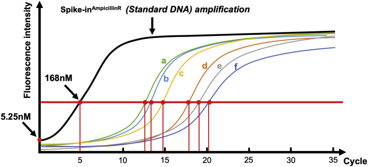  Schematic qPCR amplification of each CUT&Tagged genomic DNA sample along with the Spike-in^AmpR (Standard DNA)

  The red horizontal line indicates the targeted intensity of fluorescence when Spike-in^AmpR (Standard DNA) reached 168 nM (5 cycles). For the group of samples a, b, and c (3 conditions with the same antibody), amplification for average 13 cycles is required to reach the level of the red horizontal line, whereas Samples d, e, and f (3 conditions with a different antibody) requires approximately 19 cycles to reach the level indicated by the red horizontal line. This test qPCR is set up using 2 μL of each CUT&Tagged genomic DNA sample in a 25 μL qPCR reaction where as the actual CUT&Tag library will be generated with 20 μL of each CUT&Tagged genomic DNA sample in a 50-μL reaction (i.e., 5× more DNA). As the library prepapration will be performed with 5× higher concentration of DNA, an amplification of the DNA to 168 nM should be achieved approximately 2 cycles earlier (log₂5 ≈ 2.3). As a result, Sample a, b, and c require 13 - 2 = 11 cycles to reach 168 nM while Sample d, e, and f require 17 cycles (19-2) for library prep.

• 69.The final sample concentration for sequencing is then determined using NEBNext® Library Quant Kit for Illumina (NEB) and run as per manufacturer’s protocol.
• 70.Samples are then pooled and sequenced on NovaSeq 6000 (or equivalent platform) using 50 bp Paired-End sequencing at ∼10 M / sample. We use a S1 flowcell on an XP workflow but it can be sequenced on any flowcell (SP, S1, S2 and S4) and on any workflow (standard or regular).

Figure 11.

Bioanalyzer profiling of the tagmented DNA of CUT&Tag libraries

Data analyses after sequencing

Timing:∼4 h

A pipeline has been established in Github for users to analyze their CUT&Tag sequencing data (https://github.com/dilworthlab/CnT_pipeline_snakemake). This pipeline includes normalization of samples using Spike-in^AmpR as the default. An overview of this pipeline is provided in Figure 12. This pipeline allows for: 1) Quality Control of Raw FASTQ reads; 2) Adapter trimming; 3) Alignment (primary genome and spike-in sequences) ; 4) Post-Alignment filtering; 5) Spike-in normalization; and 6) Peak calling.

• 71.
  Prepare the software environment and download the data.

  • a.
    Install required software. A Linux-based High-Performance computing (HPC) environment is ideal for this analysis. To install the following software, set up a virtual environment within the HPC and install the required versions. 1) FastQC v0.11.9 (Babraham Bioinformatics, 2019); MultiQC >=1.9 (Ewels et al., 2016); Cutadapt >=2.6 (Martin, 2011), Bowtie2 >=2.4.1 (Langmead and Salzberg, 2012); Samtools >=1.11 (Li et al., 2009); Picard Tools >= 2.22.5 (Broad Institute); deepTools >=3.3.2 (Ramirez et al., 2016) ; SEACR >=1.3 (Meers et al., 2019); BEDtools >= 2.29.2 (Quinlan and Hall, 2010); bedToBigBed >= 2.7(Kent et al., 2002); and ChIPseeker >= 1.24.0 (Yu et al., 2015).
    A virtual environment can be set up using Conda. Conda is a convenient package management system that is included with Anaconda or Miniconda. For more information on usage documentation for condo can be consulted.
  • b.
    Download the Data. Download raw FASTQ reads to desired location and perform md5sum checks to verify the integrity of all files. With paired-end sequencing, there should be two reads (i.e., R1 and R2) per sample. For simplicity, from here onwards, these two reads can be referred to as “R1” and “R2”.
    Sample_R1.fastq.gz - ${R1}
    Sample_R2.fastq.gz - ${R2}

• 72.Quality control. Preliminary quality control checks are performed on raw FASTQ reads by running FastQC on each read individually. For more detailed information on the type of checks the tool performs, refer the documentation for FastQC.

  fastqc ${R1}

  fastqc ${R2}

  Typically, with CUT&Tag libraries, the raw reads do not always pass all QC modules (Figure 13) defined by FastQC (i.e., duplicates, overrepresented sequences, or mapped reads). This, however is not necesssarily indicative of an unusable library and hence you should proceed with further analysis. A fail in the “per base sequence quality” score would suggest that the library is not of good quality and needs to be re-made.

  • a.
    Per base sequence content
    Reads from CUT&Tag libraries usually display a non-uniform base composition at the start of the read. This is due to the sequence bias exhibited by Tn5 during transposition (Viswanadham et al., 2019).
  • b.
    Sequence duplication levels
    Since a CUT&Tag library has low complexity, the level of duplication of enriched regions is expected to be higher than for typical libraries.
    (https://www.bioinformatics.babraham.ac.uk/projects/fastqc/Help/3%20Analysis%20Modules/8%20Duplicate%20Sequences.html)
  • c.
    Overrepresented sequences

Figure 12.

An overview of the pipeline of the analyses on the raw reads of CUT&Tag DNA sequencing

The dotted arrows represent valid alternate paths within the pipeline where duplicates are not removed – this is not the preferred path.

Figure 13.

FastQC report showing failed modules that are characteristic of a typical CUT&Tag library

(A–C) (A) Per base sequence content, (B) Sequence duplication levels, and (C) Overrepresented sequences.

Not always, but sometimes there are overrepresented sequences in the library due to contaminants. These warnings can be ignored as they do not affect any of the subsequent steps.

• 73.Adaptor trimming. Illumina Nextera adaptors are trimmed from reads using Cutadapt in paired-end mode. The resulting trimmed reads are referred to as Trim.R1 and Trim.R2 respectively.

cutadapt -a CTGTCTCTTATACACATCT -A CTGTCTCTTATACACATCT \

-o $[Trim.R1] -p ${Trim.R2} ${R1} ${R2}

• 74.Alignment. After preliminary quality control and adaptor trimming, paired-end reads are aligned to both the Mus musculus (or Homo sapiens) genome and spike-in sequence using Bowtie2. The Bowtie2 output containing sequence alignment information is in SAM (Sequence Alignment Map) format. This format is however, bypassed by piping the output directly to Samtools and producing files in a storage-efficient BAM (binary version of SAM) format. The resulting BAM files are coordinate-sorted and indexed using Samtools.

  The syntax for aligning trimmed paired-end reads is as follows:

  bowtie2 {Alignment.Parameters} -× ${Genome_Index} \

  -1 ${Trim.R1} -2 ${Trim.R2} | samtools view -bS - > ${Sample}.bam

  samtools sort ${Sample}.bam -o {Sample}.coordsorted.bam

  samtools index ${sample}.coordsorted.bam

  Please note that alignment to the primary genome (mm10) and Spike-in sequence (Ampr) is done separately. Alignment parameters and genome indices for each is listed below.

  • a.
    Mus musculus
    Alignment Parameters [https://www.protocols.io/view/cut-amp-tag-data-processing-and-analysis-tutorial-bjk2kkye.html]:
    --local --very-sensitive-local --no-unal --no-mixed --no-discordant –
    phred33 -I 10 -X 700
    Genome Index: Pre-built bowtie2 indices for Mus musculus (UCSC mm10) can be retrieved directly from iGenomes (Illumina, Inc.).
  • b.
    Spike-in
    Alignment Parameters [https://www.protocols.io/view/cut-amp-tag-data-processing-and-analysis-tutorial-bjk2kkye.html]
    --end-to-end --very-sensitive --no-overlap --no-dovetail --no-
    mixed --no-discordant --phred33 -I 10 -X 700
    Genome Index: FASTA sequence of the Ampicillin resistance gene from pBlueScript II SK (+) (Addgene plasmid # 212205, GenBank ID: X52328.1) was used to build an index using bowtie2-build.
  • c.
    Alignment statistics.
    With Bowtie2, the alignment summary is printed to the standard error where it can be collected and processed. The essential metrics from Bowtie2 include:
    1) Total number of paired reads examined;
    2) Total number of mapped reads (Uniquely aligned reads + multi mapping reads). This can be used to derive the alignment rate.
    Ideally, an alignment rate between 50 and 100% is expected, however, we did observe lower rates. The reads that are not mapping either to the primary genome or to the spike-in are most probably due to amplified primers (Figure 14). For such samples, we have still observed good genomic coverage.
    MultiQC provides a convenient way of aggregating the statistics for all samples. MultiQC is run in a directory containing the appropriate log files where it will automatically detect and collect them to produce a summary report.

• 75.Post-alignment filtering.

Figure 14.

Source of unmappable reads

A bioanalyzer image shows small fragments of less than 100 bp that are likely to give rise to unmappable reads during their alignment to genome.

a. First, the resulting BAM files are filtered to only retain mapped and properly paired reads using the Samtools flag -f2.

b. Second, only uniquely aligned reads are kept by performing MAPQ-based filtering with the Samtools flag -q 10.

c. Lastly, duplicates are marked and removed using MarkDuplicates from Picard.

• 76.
  Spike-in normalization.

  • a.
    Per-sample normalization factors.
    Normalization factors for a set of libraries associated with a particular histone or transcription factor is calculated using reads mapped to the Spike-in sequence. Normalization factors for each sample is calculated as:
    Normalization Factor = Spike_min/Spike_sample
    where:
    Spike_min = No. of reads corresponding to the sample with minimum number of mapped reads within the set,
    Spike_sample = No. of total mapped reads corresponding to the sample for which the normalization factor is being calculated.
  • b.
    BigWigs and Bedgraphs

The normalization factors are used with bamCoverage from deepTools (Ramirez et al., 2016) to obtain spike-in normalized bigwig and bedgraph files. Bigwig files can be uploaded and viewed on the UCSC genome browser.

• bamCoverage --bam ${Filtered_bam} -o ${Norm}.bw \

  • --binSize 10 \
  • --scaleFactor ${NormalizationFactor} \
  • --ignoreForNormalization ‘chrM’ \
  • --extendReads
• bamCoverage --bam ${Filtered_bam} --outFileFormat bedgraph -o ${Norm}.bedgraph \

  • --binSize 10 \
  • --scaleFactor ${NormalizationFactor} \
  • --ignoreForNormalization ‘chrM’ \
  • --extendReads

where:

${Filtered_bam} = Filtered BAM files without duplicates from step 75 “Post-Alignment Filtering”.

${NormalizationFactor} = Normalization factor calculated in step 76 section a.

• 77.
  Identification of enriched regions/Peak Calling.

  • a.
    Peak Calling
    Enriched regions are identified within each sample using SEACR. In the presence of an IgG control, SEACR determines the enrichment threshold using the control IgG bedgraph file. Without a control, a FDR cut-off of 0.05 is used.
    Bash SEACR ${Target_bedgraph} ${Control_bedgraph} non stringent ${prefix}
    OR
    Bash SEACR ${Target_bedgraph} 0.05 non stringent ${prefix}
  • b.
    Filtering peaks and making bigbeds

ENCODE blacklist regions (Amemiya et al., 2019) are filtered from the peaks to remove regions prone to erroneous high signals using bedtools. The filtered peak files are converted into bigBed using bedToBigBed to enable visualization on the UCSC genome browser.

Downstream analysis

Timing:1–3 days

• 78.
  Functional Analysis and annotation of Peaks

  • a.
    Peak annotation and visualization:
    i. Annotation: Genomic features associated with peaks are obtained using ChIPseeker, an R package. Informative annotations include, but not limited to, genes and cis-regulatory elements near identified peaks.
    ii. Visualization: Tools such as deeptools can be used to visualize the enrichment profile of peaks around transcription start sites (TSSs).
  • b.
    Functional analysis of peaks:
    To study the biological relevance of enriched regions associated with a histone or transcription factor, various downstream analyses can be done using annotations from 78a. Though a detailed overview is beyond the scope of this protocol, here are some examples:
    i. It is useful to find biological themes (e.g., pathways, molecular function etc.) associated with enriched regions. Databases such as GO (http://geneontology.org/), REACTOME (https://reactome.org/) and KEGG (https://www.genome.jp/kegg/) can be queried to find overrepresented "terms" (set of genes associated with a function or pathway) within the annotated gene lists;
    ii. Motif enrichment analysis;
    iii. Various differential analyses to compare CUT&Tag libraries (e.g., WT vs KO).

Expected outcomes

After sequencing, the normal samples will contain ∼40–80% duplicates, whereas the IgG samples normally contain up to 90% duplicates. After alignment to the genome and duplicate removal, the successful CUT&Tag examples are shown in Figure 15. On the Hoxa10 locus in mouse MuSCs, H3K4me3 and H3K27me3 are enriched on different locations or genes, except for Hoxa1, which might be bivalently marked by both H3K4me3 and H3K27me3 (Figure 15A). Hoxa10 locus in human Hematopoietic Stem and Progenitor Cells (HSPCs) showed a similar pattern of H3K4me3 and H3K27me3 enrichment (Figure 15A). NELF-E bindings in MuSCs are shown as successful examples of transcription factor CUT&Tag (Figures 15A and 15B - bottom tracks).

Figure 15.

Examples of successful histone mark and transcription factor CUT&Tag assays

(A) UCSC Browser tracks showing the enrichment of H3K27me3, H3K4me3 and/or NELF-E across the HoxA locus in either murine MuSCs or human HSPCs.

(B) UCSC Browser tracks showing the enrichment of H3K27me3, H3K4me3 and/or NELF-E at the Hdgfl2 locus in murine MuSCs.

Limitations

We have experience using a large number of antibodies directed at histone marks or transcriptional regulators for looking at genomic enrichment using CUT&Tag. These conditions work well for freshly isolated MuSCs from either injured or uninjured muscles. We have not yet been able to adapt the conditions to fixed MuSCs from PFA-perfused mice. Therefore, the current form of this protocol is not suitable for histone mark profiling of true quiescent MuSCs which are isolated from PFA- or methanol-perfused mice. Further adaptations will be needed if practicing CUT&Tag assay on fixed MuSCs resulting from PFA-perfusion. Finally, users should keep in mind that the results obtained from their CUT&Tag studies will vary depending on decisions taken prior to starting the experiment. Results from MuSCs isolateds by TdT sorting might differ slightly from those obtained with ITGA7 sorting due to differences in purity, but also due to slight differences in cell identity that your selection marker defines. Pax7gCre-TdT will mark all cells that were expressing Pax7 at the time tamoxifen was administered, while ITGA7 identifies MuSCs. It is important that you plan the experiement in conditions that will allow you to study the epigenetics that best recapitulate the phenotypic conditions you are trying to understand. In our case we chose Pax7gCre-TdT cells at 30 h post injury so as to best understand MuSC activation. Please consider the optimal conditions and approach to address your research question.

Troubleshooting

Problem 1

Poor transposase/tagmentation activity of pA-Tn5 Transposase

Potential solution

Ensure the buffers are freshly prepared when purifying the enzyme. Buffer solutions should be adjusted to appropriate pH by calibrating the pH meter prior to adjusting the pH of the buffer. Inaccuarate pH could lead to loss in enzymatic activity. Similarly, Mg²⁺ is necessary for pA-Tn5 to be enzymatically active. Another potential reason could be a poor loading of ME-A and ME-B adaptors. Ensure the oligos are of good quality and are annealed properly prior to loading on to the pA-Tn5 transposase.

Problem 2

Poor staining of cell surface markers and insignificant separations of positive populations in FACS.

Potential solution

This can be caused by destruction or compromise of cell markers during digestion of the muscle tissue. This can be solved by further optimizing the digestion period as well as collagenase and dispase concentrations. Over digestion is likely to damage the cell surface markers and as a result, the digestion condition should be just sufficient to release enough MuSCs rather than over digestion. Over digestion may also cause death of MuSCs and thus an increase in the dead cell numbers.

Problem 3

Cells are not bound to Concanavalin A beads efficiently.

Potential solution

1. Replace the buffers with freshly made ones, as the MnCl₂ in Binding Buffer is critical for Concanavalin A to work. 2. Wash the cells with PBS or Wash buffer after FACS sorting to remove residual EDTA, as EDTA may decrease free Mn²⁺ through chelation and interfere with the beads to bind the cells. Actually, PBS instead of FACS buffer without EDTA is recommended for collecting cells during FACS sorting. After the cells have been mounted to the beads, the EDTA present in Antibody Buffer does not interfere with binding anymore.

Problem 4

Poor recovery of MuSCs from the hind-limb muscles.

Potential solution

Ensure that the concentration of the collagenase I and dispase II is correct. Make a fresh batch of the collagenase I/Dispase II solution.

Problem 5

Failed/poor QC on CUT&Tagged genomic DNA

Potential solution

While determing the optimal cycle number for library preparation, the QC of CUT&Tagged genomic DNA can be established. If the Ct values of IgG samples is too early to that of the histone/transcription factor specific-antibody samples, it potentially indicates poor tagmentation in antibody-specific samples. This could mean, the antibody’s poor binding to the protein of interest. Ensure the antibody dilution is at optimal concentrations. Validate the binding by immunofluorescence before proceeding to CUT&Tag with the antibody.

Resource availability

Lead contact

Further information and requests for resources and reagents should be directed to and will be fulfilled by the lead contact, F. Jeffrey Dilworth (jdilworth@ohri.ca)

Material availability

All materials mentioned in this protocol are commercially available.

Data and code availability

For data generated using this protocol refer to GEO accession: GSE150280

A pipeline has been established in Github for users to analyze their CUT&Tag sequencing data (https://github.com/dilworthlab/CnT_pipeline_snakemake).