Decision curve analysis to evaluate the clinical benefit of prediction models

Abstract

There is increased interest in the use of prediction models to guide clinical decision-making in orthopedics. Prediction models are typically evaluated in terms of their accuracy: discrimination (area-under-the-curve [AUC] or concordance index) and calibration (a plot of predicted vs. observed risk). But it can be hard to know how high an AUC has to be in order to be “high enough” to warrant use of a prediction model, or how much miscalibration would be disqualifying. Decision curve analysis was developed as a method to determine whether use of a prediction model in the clinic to inform decision-making would do more good than harm. Here we give a brief introduction to decision curve analysis, explaining the critical concepts of net benefit and threshold probability. We briefly review some prediction models reported in the orthopedic literature, demonstrating how use of decision curves has allowed conclusions as to the clinical value of a prediction model. Conversely, papers without decision curves were unable to address questions of clinical value. We recommend increased use of decision curve analysis to evaluate prediction models in the orthopedics literature.

Prediction models to guide clinical decision-making in orthopedics

There is increasing interest in using statistical prediction models to aid diagnosis or prognosis. This is at least in part because statistical prediction has been shown to be more accurate than clinician judgment, use of risk-groups or decision rules. In a typical study, clinicians were asked to predict whether a prostate cancer patient would have a positive bone scan. For any randomly selected pair of patients, one with and one without a positive bone scan, the probability that the clinician would make a correct guess (the concordance index) was only 63%, compared to 81% for a prediction model¹.

Prediction models are also of value because they allow individualization of care based on patient preference. Consider the example of surgery for pathologic spinal fractures in patients with metastatic cancer. Traditionally, the decision for surgery has relied on clinical judgment in assessing patients’ histology, extent of metastatic burden, prior treatment modalities, and life expectancy before recommending surgery². Some surgeons have adopted a decision rule, which is to treat patients with a Spinal Instability Neoplastic Score (SINS) of 13 or above³. The problem with clinician judgement or a decision rule is that they are hard to adapt to patient preference. An older, less active patient who is averse to procedures may have a higher threshold for surgery than a younger, more active patient, who wants to maximize mobility during their battle with cancer. What would be the appropriate SINS cut-off for each of these patients? A prediction model gives a quantitative estimate of absolute risk, allowing for a discussion that incorporates such preferences.

How do we know if a prediction model is a good one? Problems with traditional measures

Just as we use randomized controlled trials to evaluate treatments, we need studies to evaluate prediction models. As described in the TRIPOD statement⁴, the design of such studies is relatively straightforward: the results of the prediction model are obtained (blind to patient outcome) and compared to patient outcome (in a cohort where outcome is unaffected by the prediction model). Here we will focus on how the results of such studies are analyzed, the metrics for evaluating prediction models. The most common metric is the area-under-the-curve (AUC), obtained from the receiver operating characteristic plot of sensitivity against 1 – specificity. The AUC is a concordance index, or c-statistic, which, as described above, provides the probability that a randomly-selected patient who experienced an event received a higher risk score than a randomly-selected patient who did not. As such, it is measured on a scale from 0.5 (a “coin flip”) to 1 (perfect discrimination).

Many statisticians point out that discrimination is not enough for a model⁵. A model with high discrimination tells a patient how well their personal risk can be distinguished from another patient but does not tell them whether the actual risk they are given by a model is accurate. Indeed, if the risk predictions from a model were divided by 100 – so that even very high-risk patients were told they had little chance of disease — the concordance index would not change. We therefore also consider calibration, which describes how well a predicted risk aligns with observed risk: a model is well-calibrated if, for every 100 patients given a risk of x%, close to x actually have the event.

Calibration is generally reported in the form of a calibration plot, such as that shown in Figure 1 and Figure 2. The data are first split up into groups, typically 10, in terms of predicted risk. The observed risk in each group is then calculated along with a 95% C.I. For instance, it can be seen in Figure 1 that patients in the highest 10% of risk – the group on the far right – have a predicted risk a little above 60% (63% to be precise), but in fact very slightly less than 60% actually had the outcome.

Figure 1. Calibration plot for a hypothetical model (“Model A”) predicting pathologic spinal fracture in patients with metastatic disease.

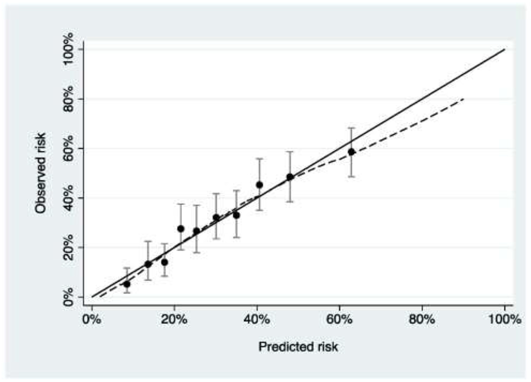
The model has good calibration, with predicted risk close to observed risk.

Figure 2. Calibration plot for a hypothetical model (“Model B”) predicting pathologic spinal fracture in patients with metastatic disease.

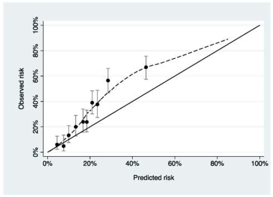
The model underestimates risk for patients at higher predicted risk.

Discrimination and calibration provide valuable information for researchers. Poor discrimination, for instance, demonstrates the predictors in a model are not strongly associated with outcome, such that researchers should consider additional predictors. Poor calibration of a model suggests genuine differences between the data set used to generate a model and the evaluation data set. For instance, a model predicting in-patient mortality for geriatric hip fracture patients was developed using a cohort of patients from the Netherlands and included, as predictors, the American Society of Anesthesiologists (ASA) score and institutional versus home residence⁶. The model might be miscalibrated when applied to a US population if there are differences between how US and Dutch clinicians score the ASA or if there are national differences in the health of individuals in institutional facilities versus living at home.

However, it is questionable whether, over and above providing information to researchers, discrimination and calibration can help clinicians decide whether or not to use a prediction model in their practice. For instance, the Dutch researchers report an AUC of 0.77 for their hip fracture mortality model. Is this high enough to warrant an orthopedic surgeon using the model to decide which patients should undergo hip fracture surgery, or would the AUC need to be closer to 0.85? Similarly, how much miscalibration would be “too much” and suggest that a model should not be used? For instance, if the model in Figure 2 had high discrimination, should it be used to aid clinical decision-making or is calibration too poor?

Decision curve analysis was developed as a method to determine whether use of a prediction model in the clinic to inform clinical decision-making would do more good than harm⁷. Here we give a brief introduction to decision curve analysis, including references and further reading, and give an overview of how it has and could be used in the orthopedic literature.

Decision curve analysis of orthopedic prediction models

To demonstrate the advantages of decision curve analysis, we will consider the example of pathologic spinal fractures in metastatic disease. In this example, early surgical intervention reduces the risk of a fracture, and hence the risk of severe pain and functional impairment. However, surgery is associated with high complication rates. Accurately predicting the risk of pathologic fractures is therefore highly beneficial in determining who to treat and who to observe until symptoms progress and risk of fractures increases. Typically, patients are recommended for surgery on the basis of high SINS or imaging results.

We will use a hypothetical example for illustrative purposes. Suppose there are two prediction models, model A and model B, that have been developed by two different teams to predict a patient’s risk of pathologic fractures within the next 6 months using variables such as SINS and history of osteoporosis as predictors. A study is conducted to evaluate both models on an independent cohort of 1000 patients who were eligible for surgery on the basis of SINS or imaging but in fact never underwent an operation. The investigators report AUCs of 0.715 vs. 0.758 for model A and model B with calibration as shown in Figures 1 and 2. The obvious problem is that calibration is superior for model A but discrimination is better for model B. It is hard to tell whether the miscalibration shown for model B in Figure 2 offsets the advantages of superior AUC. One might also reasonably ask the question whether either model should be used at all.

This is exactly the sort of problem that decision curve analysis was designed to address. We start from the idea that, in order to know whether the benefits of a model outweigh the harms, we have to put some numbers on benefit and harm. To do so, we need to think about the threshold probability of disease. This is defined as the minimum probability of disease (in this case, future pathologic fracture) at which a decision-maker — doctor or patient - would opt for an intervention (in this case, surgery). Consider that, if a patient were told that the probability of pathologic fractures was 1%, the discomfort and risks of surgery would certainly outweigh any benefit from reduced risk of fracture. Conversely, if the patient were told the risk of fractures was 99%, they would certainly choose to have surgery. If we were to gradually increase the probability of pathologic fractures from 1% to 99%, there would come a point where the patient would be unsure whether or not to have surgery. We call this point p_t, the threshold probability and it is directly linked to how the consequences of the decision are weighted. For example, imagine that a patient stated that they would opt for surgery if their risk of pathologic fractures were 25% or higher but not if their risk were less than 25%. A 25% risk of fracture is a 75% chance of no fracture, a 3:1 ratio. Therefore, a patient with a p_t of 25% thinks that the benefits of early surgical intervention for pathologic fractures are worth three times more than the harms of unnecessary surgery.

Decision curve analysis applies this intuition to account for clinical consequences and thereby quantify benefits and harms. The threshold probability p_t is used in a simple formula to calculate the net benefit of the prediction model. The idea of net benefit analogous to profit, where revenue and costs are put on the same scale and compared directly. As an illustration, take the case of a wine importer who pays €1m to buy wine in France and then sells it for $1.5m in the United States. To determine the profit, the exchange rate between euros and dollars is required to put revenue and cost on the same scale using the formula: profit = income — expenses × exchange rate. If €1 is worth $1.25, then profit is $1.5m - €1m × 1.25 = $250,000. Applying this principle to the medical setting, profit is true positives – the model accurately identifies a patient who is destined to get a fracture and recommends risk-reducing surgery – and cost is false negatives: patients who would not get a fracture but for whom the model recommends surgery nonetheless. The exchange rate is derived from the threshold probability as described above. This gives the formula below, where N is the total number of patients

$$NetBenefit=\frac{Truepositives-Falsepositives\times \frac{p_t}{1-p_t}}{N}$$

In table 1, we apply net benefit to the study where model A and B were applied to the cohort of 1000 patients. We also include two clinical strategies that are alternatives to using a model: “treat none” or “treat all”. Model A has a higher net benefit than model B, despite model B having better discrimination, and it is also superior to recommending that either all or no patient gets surgery. Hence using model A to choose who gets surgery would lead to the best clinical outcome.

Table 1. Net benefit of the two models for predicting facture.

Net benefit is given at a threshold probability of 25% along with that for the clinical alternatives of recommending surgery for all or no patients.

Strategy	True positives: patients recommended for surgery who would otherwise get a fracture	False positives: patients recommended for surgery who will not get a fracture	Net benefit
Recommend surgery for all patients	306	694	(306–694 x (0.25 ÷ 0.75)) ÷ 1000 = 0.0747
Recommend surgery if risk ⩾ 25% according to Model A	240	335	(240–335 x (0.25 ÷ 0.75)) ÷ 1000 = 0.128
Recommend surgery if risk ⩾ 25% according to Model B	136	84	(136 – 84 x (0.25 ÷ 0.75)) ÷ 1000 = 0.108
Surgery for no patients	0	0	(0 – 0 x (0.25 ÷ 0.75)) ÷ 1000 = 0

An obvious problem with this approach is that we fixed the threshold probability at 25%. There may be some patients who are more averse to surgery – and who would want to avoid surgery unless they really needed it – or some doctors who are more aggressive. So what we do in decision curve analysis is to vary the threshold probability p_t across a reasonable range and then calculate net benefit for each strategy at every level of threshold probability p_t. Figure 3 shows the decision curve using a range for threshold probabilities from 20% to 50% on the grounds that, given the harms of surgery, few doctors would recommend surgery for a patient with a risk less than 20% and, on the other hand, few patients would be prepared to risk a greater than 50:50 chance of a fracture and not get surgery. The decision curve shows that model A has the highest net benefit across the whole range of reasonable threshold probabilities. What we can conclude is that we would improve clinical outcome if we were to use model A to decide which patients should undergo surgery rather than treating all patients, no patients or using model B to decide. For more on understanding net benefit, see Vickers et al.⁸

Figure 3. Decision curve analysis for two hypothetical models predicting pathologic spinal fracture in patients with metastatic disease.

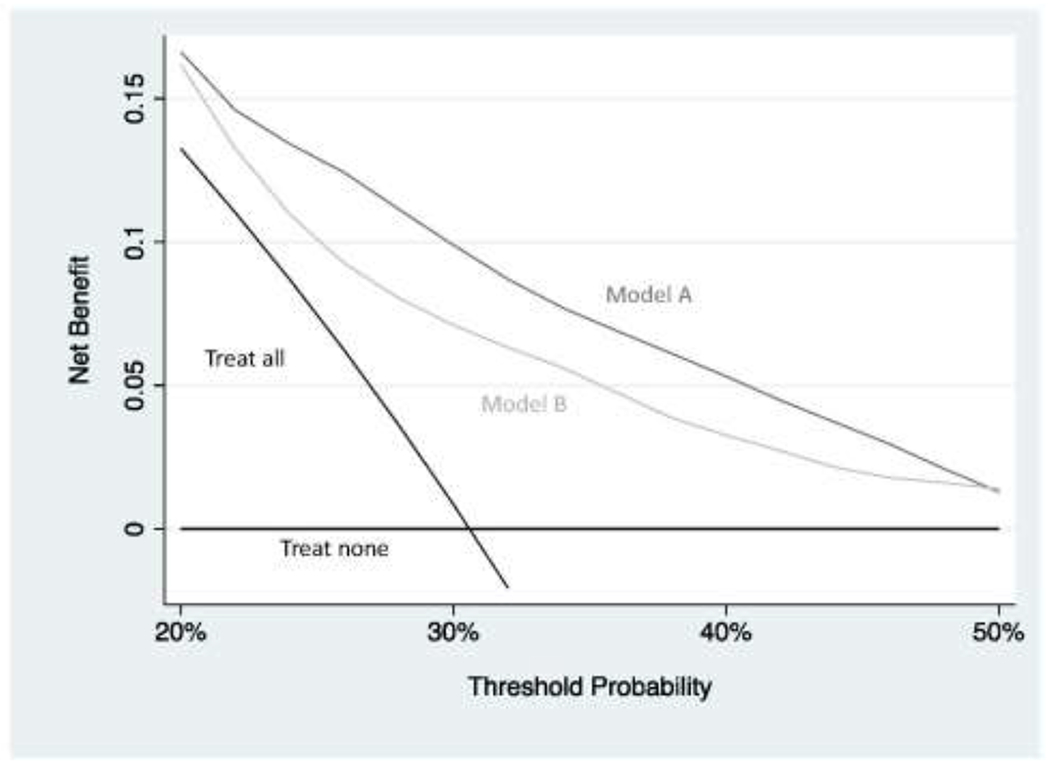
Model B has better discrimination (0.715 vs. 0.758) but is miscalibrated(figure 2). The decision curve shows that the miscalibration offsets improved discrimination: model A has a higher net benefit compared to model B, as well in comparison to the clinical default strategies of “treat all” or “treat none”, over the entire range of reasonable threshold probabilities. Using model A to decide which patients should receive surgery would therefore lead to the best clinical outcomes.

It is not always the case that a model is clinically useful, even if it is well calibrated and has good discrimination. Consider the example of anemia after major orthopedic surgery, the prevalence of which can be as high as 85%⁹. It has been proposed that patients should be given intravenous iron to reduce the risk of anemia¹⁰. But postoperative anemia is actually relatively predictable in terms of age, sex, preoperative hemoglobin and type of fracture, so we might imagine that a group of investigators build a prediction model and then propose that intravenous iron is only given to patients at higher risk.

Let us assume that the model is perfectly calibrated and has a high discrimination of 0.80. Figure 4 shows the decision curve for a simulated data set for such a model. It can be seen that the model is not better than the strategy of just giving all patients intravenous iron as a standard prophylactic measure unless the threshold probability is 50% or higher. Of course, given that postoperative anemia is associated with important complications, including infection, delayed discharge and even mortality⁹, and intravenous iron is a relatively safe intervention, we would probably give iron if the risk of anemia was relatively low, 5% or 10%. The decision curve shows that the model is not of value in this range. The problem is that the prevalence of postoperative anemia is very high (we can actually see this on the decision curve: the curve for “treat all” crosses that for “treat none” at the prevalence). A model would have to be extremely accurate to move a patient’s risk from the average (85%) all the way down to below a threshold of 5 or 10%.

Figure 4. Decision curve analysis for a model predicting anemia after hip surgery.

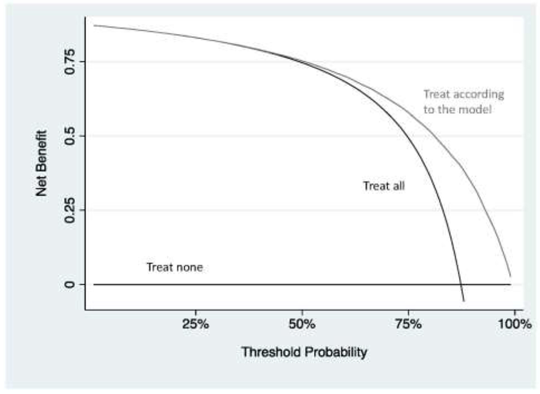
The model only has benefit at threshold probabilities that are irrelevant for the clinical scenario. Note that, for didactic purposes and unlike a typical decision curve, the entire range of threshold probabilities is shown.

Decision curve analysis can also show that models can actually be harmful. In Figure 5, which is based on the pathologic fracture example, the net benefit for the model is lower than for “treat all” for some probability thresholds. In other words, using the model would be worse than just doing the surgery in all eligible patients. This can happen if the model is miscalibrated. It is not hard to see how a patient can make a bad decision to avoid surgery if they are told that they are at lower risk than they truly are.

Figure 5. Decision curve analysis for a hypothetical model predicting pathologic spinal fracture in patients with metastatic disease.

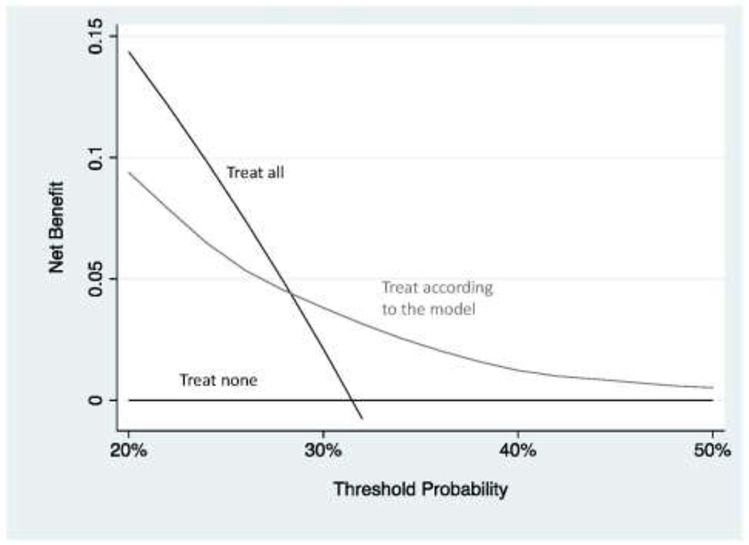
The model leads to worse outcome than treating all patients at some threshold probabilities and so using the model in clinical practice would lead to harm.

How are models evaluated in the orthopedics literature?

Several prediction models in the orthopedic literature have presented measures of accuracy without a decision curve analysis. For instance, one group of investigators developed several models to predict rotator cuff tears, the idea being to reduce the burden of further invasive and expensive tests such as arthrograms and magnetic resonance imaging¹¹. However, because the authors only report measures such as the AUC, and sensitivity / specificity, we do not know whether we would improve clinical outcome were we to use the model to aid decision-making about work-up. Similarly, a model for predicting metastasis in osteosarcoma, reported a concordance index of 0.80¹². The authors claimed that this was a good level of discrimination and that use of the model could improve patient outcomes by individualizing the aggressiveness of treatment according to risk of metastasis. But again, we are left with wondering whether a concordance index of 0.80 is high enough to warrant changes to life-and-death decisions about surgery and chemotherapy.

In contrast, a different study group addressed a similar problem but reported a decision curve as well as accuracy metrics. Interestingly, although a model including radiomics data had better discrimination for prediction of osteosarcoma outcomes, AUCs of 0.84 vs. 0.73, it did not show higher net benefit unless threshold probabilities were relatively high, above 40% or so. This demonstrates the value of a decision curve analysis to complement reporting of calibration and discrimination¹³.

Karhade et al. evaluated models to predict 90-day and one-year survival for patients with spinal metastasis and thereby inform whether to undergo palliative surgery. The best model had an AUC of 0.83 and 0.89 for 90 day and one-year survival respectively; it was well-calibrated for the former endpoint but less so for the latter. Again, it is difficult to know whether these levels of discrimination and calibration are sufficient to warrant use of the model to aid decision-making. However, the authors also applied decision curve analysis and found good net benefit across a wide-range of threshold probabilities¹⁴.

Decision curve analysis was also applied in a study investigating whether an osteogenomic profile could improve the assessment of fracture risk in patients considering treatment for osteoporosis. The authors were able to demonstrate that adding the genomic profile to a standard risk prediction improved net benefit. They also used the net benefit results to quantify the improvement affording by the genomic approach, the equivalent of detecting an additional 3 fractures in women and 11 in men per 1000 patients with no increase in false positives. This allows the reader to consider whether genomic profiling would be clinically worthwhile¹⁵. For an example of decision curve analysis applied to prediction model for amputation, see Forsberg et al.¹⁶

Conclusion

Unlike traditional biostatistical methods, which only evaluate the accuracy of a model, decision curve analysis can tell us whether using a model to aid clinical decision-making would improve outcomes for our patients. Decision curve analysis is now widely used in the literature – the primary publication has over 1500 citations – and has been recommended in editorials in several major journals including JAMA, BMJ, Journal of Clinical Oncology and Annals of Internal Medicine ^17–20. Didactic papers on creating and interpreting decision curves have been published^8,21,22 and are summarized, along with statistical code, tutorials and data sets, at www.decisioncurveanalvsis.org. We recommend increased use of decision curves to evaluate prediction models in the orthopedics literature.

References

- 1.Kattan MW, Yu C, Stephenson AJ, Sartor O, Tombal B. Clinicians versus nomogram: predicting future technetium-99m bone scan positivity in patients with rising prostate-specific antigen after radical prostatectomy for prostate cancer. Urology. 2013;81(5):956–961. [DOI] [PubMed] [Google Scholar]
- 2.Harel R, Angelov L. Spine metastases: current treatments and future directions. Eur J Cancer. 2010;46(15):2696–2707. [DOI] [PubMed] [Google Scholar]
- 3.Fourney DR, Frangou EM, Ryken TC, et al. Spinal instability neoplastic score: an analysis of reliability and validity from the spine oncology study group. J Clin Oncol. 2011;29(22):3072–3077. [DOI] [PubMed] [Google Scholar]
- 4.Moons KG, Altman DG, Reitsma JB, et al. Transparent Reporting of a multivariable prediction model for Individual Prognosis or Diagnosis (TRIPOD): explanation and elaboration. Ann Intern Med. 2015;162(1):W1–73. [DOI] [PubMed] [Google Scholar]
- 5.Van Calster B, McLernon DJ, van Smeden M, Wynants L, Steyerberg EW. Calibration: the Achilles heel of predictive analytics. BMC Med. 2019;17(1):230. [DOI] [PMC free article] [PubMed] [Google Scholar]
- 6.Schuijt HJ, Smeeing DPJ, Würdemann FS, et al. Development and internal validation of a prediction model for in-hospital mortality in geriatric hip fracture patients. J Orthop Trauma. 2020. [DOI] [PubMed] [Google Scholar]
- 7.Vickers AJ, Elkin EB. Decision curve analysis: a novel method for evaluating prediction models. Med Decis Making. 2006;26(6):565–574. [DOI] [PMC free article] [PubMed] [Google Scholar]
- 8.Vickers AJ, van Calster B, Steyerberg EW. A simple, step-by-step guide to interpreting decision curve analysis. Diagn Progn Res. 2019;3:18. [DOI] [PMC free article] [PubMed] [Google Scholar]
- 9.Spahn DR. Anemia and patient blood management in hip and knee surgery: a systematic review of the literature. Anesthesiology. 2010;113(2):482–495. [DOI] [PubMed] [Google Scholar]
- 10.Steuber TD, Howard ML, Nisly SA. Strategies for the Management of Postoperative Anemia in Elective Orthopedic Surgery. Ann Pharmacother. 2016;50(7):578–585. [DOI] [PubMed] [Google Scholar]
- 11.Lu HY, Huang CY, Su CT, Lin CC. Predicting rotator cuff tears using data mining and Bayesian likelihood ratios. PLoS One. 2014;9(4):e94917. [DOI] [PMC free article] [PubMed] [Google Scholar]
- 12.Sheen H, Kim W, Byun BH, et al. Metastasis risk prediction model in osteosarcoma using metabolic imaging phenotypes: A multivariable radiomics model. PLoS One. 2019;14(11):e0225242. [DOI] [PMC free article] [PubMed] [Google Scholar]
- 13.Wu Y, Xu L, Yang P, et al. Survival Prediction in High-grade Osteosarcoma Using Radiomics of Diagnostic Computed Tomography. EBioMedicine. 2018;34:27–34. [DOI] [PMC free article] [PubMed] [Google Scholar]
- 14.Karhade AV, Thio Q, Ogink PT, et al. Predicting 90-Day and 1-Year Mortality in Spinal Metastatic Disease: Development and Internal Validation. Neurosurgery. 2019;85(4):E671–e681. [DOI] [PubMed] [Google Scholar]
- 15.Ho-Le TP, Tran HTT, Center JR, Eisman JA, Nguyen HT, Nguyen TV. Assessing the clinical utility of genetic profiling in fracture risk prediction: a decision curve analysis. Osteoporos Int. 2020. [DOI] [PubMed] [Google Scholar]
- 16.Forsberg JA, Potter BK, Wagner MB, et al. Lessons of War: Turning Data Into Decisions. EBioMedicine. 2015;2(9):1235–1242. [DOI] [PMC free article] [PubMed] [Google Scholar]
- 17.Fitzgerald M, Saville BR, Lewis RJ. Decision curve analysis. Jama. 2015;313(4):409–410. [DOI] [PubMed] [Google Scholar]
- 18.Kerr KF, Brown MD, Zhu K, Janes H. Assessing the Clinical Impact of Risk Prediction Models With Decision Curves: Guidance for Correct Interpretation and Appropriate Use. J Clin Oncol. 2016;34(21):2534–2540. [DOI] [PMC free article] [PubMed] [Google Scholar]
- 19.Vickers AJ, Van Calster B, Steyerberg EW. Net benefit approaches to the evaluation of prediction models, molecular markers, and diagnostic tests. Bmj. 2016;352:16. [DOI] [PMC free article] [PubMed] [Google Scholar]
- 20.Localio AR, Goodman S. Beyond the usual prediction accuracy metrics: reporting results for clinical decision making. Ann Intern Med. 2012;157(4):294–295. [DOI] [PubMed] [Google Scholar]
- 21.Capogrosso P, Vickers AJ. A Systematic Review of the Literature Demonstrates Some Errors in the Use of Decision Curve Analysis but Generally Correct Interpretation of Findings. Med Decis Making. 2019;39(5):493–498. [DOI] [PMC free article] [PubMed] [Google Scholar]
- 22.Van Calster B, Wynants L, Verbeek JFM, et al. Reporting and Interpreting Decision Curve Analysis: A Guide for Investigators. Eur Urol. 2018;74(6):796–804. [DOI] [PMC free article] [PubMed] [Google Scholar]