Abstract
Starting from Wuhan in China at the end of 2019, coronavirus disease (COVID-19) has propagated fast all over the world, affecting the lives of billions of people and increasing the mortality rate worldwide in few months. The golden treatment against the invasive spread of COVID-19 is done by identifying and isolating the infected patients, and as a result, fast diagnosis of COVID-19 is a critical issue. The common laboratory test for confirming the infection of COVID-19 is Reverse Transcription Polymerase Chain Reaction (RT-PCR). However, these tests suffer from some problems in time, accuracy, and availability. Chest images have proven to be a powerful tool in the early detection of COVID-19. In the current study, a hybrid learning and optimization approach named CovH2SD is proposed for the COVID-19 detection from the Chest Computed Tomography (CT) images. CovH2SD uses deep learning and pre-trained models to extract the features from the CT images and learn from them. It uses Harris Hawks Optimization (HHO) algorithm to optimize the hyperparameters. Transfer learning is applied using nine pre-trained convolutional neural networks (i.e. ResNet50, ResNet101, VGG16, VGG19, Xception, MobileNetV1, MobileNetV2, DenseNet121, and DenseNet169). Fast Classification Stage (FCS) and Compact Stacking Stage (CSS) are suggested to stack the best models into a single one. Nine experiments are applied and results are reported based on the Loss, Accuracy, Precision, Recall, F1-Score, and Area Under Curve (AUC) performance metrics. The comparison between combinations is applied using the Weighted Sum Method (WSM). Six experiments report a WSM value above 96.5%. The top WSM and accuracy reported values are 99.31% and 99.33% respectively which are higher than the eleven compared state-of-the-art studies
Keywords: Computed Tomography (CT), Convolutional Neural Network (CNN), COVID-19, Data Augmentation (DA), Harris Hawks Optimization (HHO), Transfer Learning (TL)
1. Introduction
The novel Coronavirus (COVID-19) has led to a global crisis due to its rapid spread from one person to another (Zaim, Chong, Sankaranarayanan, & Harky, 2020). This crisis began in Wuhan in China in December 2019. The World Health Organization (WHO) declared the novel coronavirus caused by SARS-CoV-2 as a pandemic in January 2020 (Xu & Li, 2020). The common symptoms of COVID-19 include, but are not limited to, fever, dry cough, sleepiness, and loss of smell and taste (Wang, Kang, Liu, & Tong, 2020). Severe cases may suffer from the difficulty of breathing and multi-organ damage (Zaim et al., 2020).
During the first days of the infection, it was very difficult to examine and diagnose the COVID-19 using the Reverse Transcription Polymerase Chain Reaction (RT-PCR) test, which is the standard test for confirming the COVID-19 positive patients (Li, Yao, et al., 2020). RT-PCR also consumes time and money (Gupta, Anjum, Gupta, & Katarya, 2021). In this case, patients with a late diagnosis can develop severe symptoms due to the delay in treatment. These patients are also a main source of infection. So, it is necessary to diagnose patients and isolate them as early as possible to stop the disease spread (Bahgat, Balaha, AbdulAzeem, & Badawy, 2021).
In recent studies, medical imaging including Chest Computed Tomography (CT) and chest X-ray have proven to be a valuable method for COVID-19 detection (Ozturk et al., 2020, Rubin et al., 2020). In the investigation of the COVID-19 patients, CT images are powerful for detecting COVID-19 since they are more sensitive than X-ray images (Wong et al., 2020). While this technique has some advantages over the current RT-PCR test regarding the early detection of the COVID-19 and accuracy, this approach requires experts to understand the chest images (Gupta et al., 2021, Nour et al., 2020).
The current evolution in Artificial Intelligence (AI) leads to the appearance of Deep Learning (DL) approaches (Abdulazeem, Balaha, Bahgat, & Badawy, 2021). DL can deal with huge datasets containing millions of data easily and efficiently (Najafabadi, Villanustre, Khoshgoftaar, Seliya, Wald, & Muharemagic, 2015). The commonly used deep learning approach in the field of medical imaging is the Convolutional Neural Network (CNN) (Huynh, Li, & Giger, 2016). Due to their remarkable ability to extract features from images, CNN has been successfully used in image-related problems (Xu, Ren, Liu, & Jia, 2014). CNN has also proven to have a superior performance in classification problems (Zhang et al., 2018). Applications of CNNs in medical imaging include, but are not limited to, skin cancer classification (Dorj, Lee, Choi, & Lee, 2018), lung tumor detection (Kasinathan et al., 2019), pancreatic ductal adenocarcinoma (Zhang, Lobo-Mueller, et al., 2020), and breast cancer diagnosis (Gao et al., 2018). Thus, CNN can be used for the detection of COVID-19 patients from either Chest X-ray or CT images accurately and almost at no time (Marques, Agarwal, & de la Torre Díez, 2020).
Nowadays, metaheuristic algorithms are powerful for solving different optimization problems. The main reason behind this is their flexibility (Yousri et al., 2021). Examples of these algorithms are Genetic Algorithms (GA) (Holland, 1992), Particle Swarm Optimization (PSO) (Kennedy & Eberhart, 1995), Cuckoo Search (CS) algorithm (Yang & Deb, 2010), Grasshopper Optimization Algorithm (GOA) (Balaha and Saafan, 2021, Saremi et al., 2017), and Gray Wolf Optimizer (GWO) (Mirjalili, Mirjalili, & Lewis, 2014). Also, many learning techniques have been used to improve the performance of the metaheuristic algorithms (El-Gendy et al., 2020, Feng et al., 2018, Li, Li, Tian, and Xia, 2019, Li, Li, Tian, and Zou, 2019, Li and Wang, 2021, Li, Wang, and Alavi, 2020, Li, Wang, Dong, et al., 2021, Li, Wang, and Gandomi, 2021, Li, Wang, and Wang, 2021, Li, Xiao, et al., 2020, Nan et al., 2017, Saafan and El-Gendy, 2021, Wang, Deb, et al., 2016).
An interesting algorithm is the Harris Hawks Optimization (HHO) introduced by Heidari et al. (2019). HHO is a population-based, nature-inspired optimization algorithm that mimics the chasing behavior of Harris’ hawks. This behavior is called the surprise pounce, in which several hawks cooperatively attack a prey, usually a rabbit, from different directions in a bid to shock it. HHO algorithm works similarly. There is an interest in the use of HHO in several applications (Bao et al., 2019, Chen et al., 2020, Golilarz et al., 2019, Jia et al., 2019).
In the current study, a hybrid Harris hawks optimization deep learning approach for the COVID-19 detection (CovH2SD) is proposed to diagnose positive COVID-19 patients using the chest CT images. The proposed approach consists of two major stages (1) Fast Classification Stage (FCS) and (2) Compact Stacking Stage (CSS). FCS makes use of nine fine-tuned pre-trained CNNs, namely ResNet50 and ResNet101 (He, Zhang, Ren, & Sun, 2016), VGG16, VGG19 (Simonyan & Zisserman, 2014), Xception (Chollet, 2017), MobileNet (Howard et al., 2017), MobileNet-v2 (Sandler, Howard, Zhu, Zhmoginov, & Chen, 2018), DenseNet121, and DenseNet169 (Balaha, Ali, Youssef, et al., 2021, Huang et al., 2017).
The usage of the pre-trained methods via transfer learning (TL) can reduce the computational cost and offer more accurate results especially in the case of the COVID-19, in which there is not enough data to build CNNs from scratch. Here, we used the HHO algorithm to optimize these pre-trained models to increase the accuracy of detection. In CSS, alternative stacking configurations of the different models are made in order to choose the most suitable model. CovH2SD maps the different stacking configurations into a proposed Quality Space (QS), calculates the rank of each model, and the models with the most significant ranks are used to classify COVID-19. CovH2SD is first trained and tested to classify chest CT images into patient and normal classes. The prime contributions of the current research can be summarized into:
-
1.
Proposing a hybrid Harris hawks optimization deep learning approach for the COVID-19 detection (CovH2SD) using the chest CT images.
-
2.
Applying transfer learning using nine pre-trained convolutional neural network models.
-
3.
Injecting Harris haws optimization in the learning process to select the optimal configurations for each model.
-
4.
Presenting a stacking mechanism from the optimized models.
-
5.
The proposed approach is benchmarked against other state-of-the-art models.
The rest of the paper is organized as follows. Section 2 gives a quick survey about the related models for the detection of COVID-19. Section 3 illustrates the basic knowledge needed to understand the proposed model. The techniques used to build the proposed CovH2SD and its structure are explained in Section 4. The experimental results and their discussion, and the comparative study of our proposed approach are discussed in Section 5. Section 6 presents the conclusion and future works.
2. Related work
In this section, we introduce a quick overview of the latest research regarding the use of artificial intelligence in the detection of COVID-19 from chest images, either X-ray or CT.
Ozturk et al. (2020) proposed “DarkCovidNet”, a deep learning model to classify COVID-19 and pneumonia from X-ray scan images. They classified images into “COVID-19” and “Normal” for binary classification, and into “COVID-19”, “Pneumonia Bacterial”, “Pneumonia Viral”, and “Normal” for multi-class classification. They achieved an accuracy of 89.6%, 95%, and 98.08% for four, three, and binary class classifications, respectively.
Apostolopoulos and Mpesiana (2020) used the TL-based CNN models on a database of X-ray images including COVID-19 disease, bacterial pneumonia diseases, and normal images; obtaining an accuracy of 98.75% for VGG19 and 97.40% for MobileNetV2.
Hemdan, Shouman, and Karar (2020) proposed “COVIDX-Net”, a deep learning model including seven different architectures to detect the COVID-19 from chest X-ray images. The best-achieved accuracy was 90% from both VGG19 and DenseNet201. Khan, Shah, and Bhat (2020) proposed a novel CNN model called “CoroNet” built using Xception architecture. They could achieve an average accuracy of 89.6%.
Toraman, Alakus, and Turkoglu (2020) proposed a Convolutional “CapsNet” model for the COVID-19 detection from X-ray images and applied it to both binary classification and multi-class classification, achieving an accuracy of 97.24% and 84.22%, respectively.
Gupta et al. (2021) proposed “InstaCovNet-19”, an integrated stacked deep convolution network. The architecture of the model is based on the pre-trained models such as ResNet101, Xception, and InceptionV3. They classified Chest X-ray images into “COVID-19”, “Pneumonia”, and “Normal” (multi-class classification), and “COVID-19” and “Normal” (binary classification), achieving an accuracy of 99.08% and 99.53%, respectively.
Furthermore, Gour and Jain (2020) proposed a stacked model consisting of the VGG19 model and developed a model called “CovNet30” consisting of a 30-layered CNN model. They applied the model on chest X-ray images and achieved an accuracy of 92.74%. Mangal et al. (2020) proposed “CovidAID”, a deep neural network-based model for detecting COVID-19 in chest X-ray, achieving an accuracy of 90.5%.
Aslan, Unlersen, Sabanci, and Durdu (2020) used a hybrid approach by applying TL to AlexNet architecture and adding a Bidirectional Long Short-Term Memories layer to detect COVID-19 in X-ray images. They could achieve an accuracy of 98.70%. Zhang, Liu, et al. (2020) proposed a CNN model based on ResNet18 architecture for multi-class classification of COVID-19 using CT images. They achieved an accuracy of 92.49%.
Ardakani, Kanafi, Acharya, Khadem, and Mohammadi (2020) applied CNN structures to detect COVID-19 in CT images. The best performance was achieved by ResNet101 with an accuracy of 99.51% and Xception with an accuracy of 99.20%.
Zhang, Zhang, and Zhu (2021) proposed an attention network for the diagnosis of COVID-19 using a convolutional block attention module. They also used Grad-CAM to give an explicable diagnosis. They achieved an accuracy of , and using two different datasets.
In the work proposed by Zhang, Zhang, Zhang, and Wang (2021), they proposed a multiple-input deep convolutional attention network using a convolutional block attention module. There are two inputs to the model, one for 3D chest CT image, and the other for 2D X-ray image. They could achieve an accuracy of .
The previous studies are just examples of the existing research in the application of artificial intelligence to the diagnosis of COVID-19 patients. As seen from the studies, the most important factors affecting the accuracy are the structure of the model and the dataset used in the learning process. What distinguishes this study from all of the presented works is that HHO is used to select the optimal hyperparameters for the different CNN pre-trained models. We believe that we can achieve better results by stacking the optimized pre-trained models. In the next section, we discuss the basic knowledge, concepts, and algorithms required to implement the suggested approach.
3. Background
In the current section, all the basic knowledge used in the suggested approach about Convolutional Neural Networks, Transfer Learning, and Stacking are explained. Moreover, we demonstrate the important aspects of the Harris Hawks Optimization algorithm.
3.1. Convolutional Neural Networks (CNN)
The main inspiration behind the artificial neural network (ANN) is the human nervous system and the structure of the cerebral cortex. A simple ANN consists of at least one neuron. It mimics the natural neuron, thus it has two main functions: summing the different inputs, and the result passes through an activation function. The activation function is used to output a predefined value based on a threshold (Wang, 2003).
The structure of ANN is usually in the form of layers. Each layer contains a different number of neurons. This type of ANN is called a feedforward neural network. These networks consist basically of an input layer, an output layer, and one or more hidden layers. The network can learn to classify, recognize, and identify different objects by adjusting the weights of the hidden layers (Livingstone, 2008). The algorithm used for learning in feedforward neural networks is called the back-propagation algorithm. The adaptation of the weights is done in a way that a certain loss (cost) function is to be minimized. In summary, the ANN objectives can be described in two steps: (1) finding the ideal values of the different weights, while (2) minimizing a certain loss function (Abiodun et al., 2018).
It is worth mentioning that, other algorithms have been proposed to overcome the disadvantages of traditional learning algorithms such as the time taken by the network to learn, the dependency of the learning process on the learning rate parameter, and the risk of falling in local minimum (Cui et al., 2018, Wang et al., 2013, Wang, Lu, et al., 2016, Yi et al., 2016).
However, when dealing with images and computer vision problems, there is an incredible number of features to extract and learn. Feedforward neural networks are not powerful to deal with this massive data. CNNs are designed to deal with images (Albawi, Mohammed, & Al-Zawi, 2017). They depend on the convolutional operation that can be processed in parallel. CNNs can learn only the important features from images with much fewer connections and parameters (Krizhevsky, Sutskever, & Hinton, 2012). To improve the performance of CNN, many factors should be considered; including the initialization of weights, the optimization algorithm used, the learning rate, the type of chosen activation function, the proper choice of the loss function, and the number of epochs (Qin, Yu, Liu, & Chen, 2018). The information (extracted features) passes through the different layers of the CNN (e.g. convolution, pooling, and fully-connected (FC) layers) (Yamashita, Nishio, Do, & Togashi, 2018).
Convolution Layer: Convolution means to convolve a matrix (i.e. kernel) that slides through the entire input image and is multiplied to that image to extract some features of this image. Thus, the convolution layer performs feature extraction. Neurons at this layer are called filters, and they take the inputs and convert them into output feature maps. Mathematically, the filter shifts from left to right until reaching the maximum width of the image. Then, the filter begins at the left-most pixel of the next row. The process continues till the entire image is completed (Balaha, Ali, & Badawy, 2021).
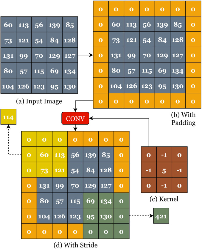
The convolution of a image by a kernel is illustrated in Fig. 1.
Fig. 1.
Graphical Illustration of the Convolution Process.
The original image in Fig. 1(a) is padded by zeros as shown in Fig. 1(b). Padding helps to work with the boundary pixels. A stride of is applied as shown in Fig. 1(d). The stride is the size of the sliding window in both directions. The result of this process is a matrix called the feature map. The size of a feature map is calculated based on the convolutional size, stride, padding, and filter size as shown in Eq. (1).
| (1) |
where is the input width, is the input height, is the convolutional filter width, is the convolutional filter height, is the convolutional padding width, is the convolutional padding height, is the convolutional stride width, is the convolutional stride height, and is the number of convolutional filters.
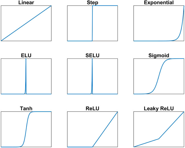
Activation Functions: The output of the convolution layer passes through an activation function. The reason behind that is to calculate the output of the neural network. Depending on the type of the used activation function, the output of the network changes. So, the choice of a suitable activation function is required to get the correct response. This choice depends mainly on the type of the problem, this means that every problem can have the right activation function. There are different types of activation functions. Two main categories exist, which are: linear and nonlinear activation functions. The output of each type is different, and hence we have different options for the outputs of the neurons. Table 1 shows some different well-known activation functions and they are summarized in Fig. 2.
Table 1.
The different activation functions.
| Function | Equation |
|---|---|
| Linear | |
| Step | |
| Exponential | |
| ELU | |
| SELU | |
| Sigmoid | |
| Tanh | |
| ReLU | |
| Leaky ReLU |
Fig. 2.
Graphical Illustration of the Activation Functions.
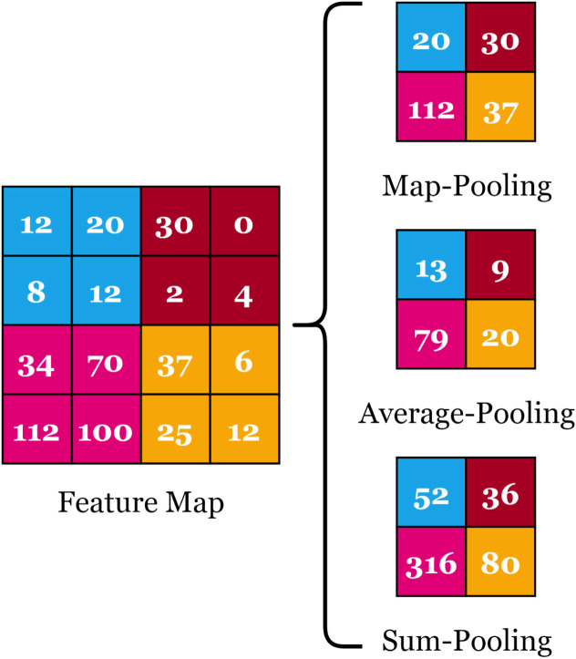
Pooling Layer: Pooling layers are used to reduce the dimensions of the feature maps. It is preferred to add a pooling layer after every convolution layer to reduce the computational complexity and help overcome the overfitting problem. There are different types including max-, average- (i.e. mean-), and sum-pooling. In max-pooling, the maximum value is used. In average-pooling, the average value is calculated while in sum-pooling, the summation is applied. Fig. 3 presents a graphical illustration of the different pooling types.
Fig. 3.
Graphical Illustration of the Pooling Layer Types.
The output size of a pooling layer is calculated based on the input size, stride, and pooling size as shown in Eq. (2).
| (2) |
where is the pooling width, is the pooling height, is the pooling stride width, is the pooling stride height, and is the number of input filters.
Fully-Connected (FC) Layer: The output of the pooling layer is then flattened. Flattening is the process of converting a matrix into a vector. This vector is fed to the fully connected layer. FC Layers are the last layers in the CNN. They are simply feed-forward neural networks.
Dropout: It is simply to drop out some neurons in a neural network. The CNN is supposed to be fully connected. However, sometimes it is useful to randomly set the output of some hidden layer neurons to at the training phase. The introduction of dropout can cause the weights of the network to be larger than normal. As a solution to this problem, it is recommended to scale the weights by a chosen suitable dropout rate. The use of dropout is useful because it helps avoid overfitting in networks.
Parameters Optimizers: The selection of the proper parameters’ optimizer plays an important role in evaluating the performance of the CNN. It is necessary to choose a suitable optimizer to converge faster and avoid the local minima. There are different types of optimizers for the CNN such as Adaptive Momentum (Adam) (Kingma & Ba, 2014), Adaptive Gradient (AdaGrad) (Luo, Xiong, Liu, & Sun, 2019), Nesterov Adaptive Momentum (NAdam) (Dozat, 2016), Adaptive Delta (AdaDelta) (Dogo, Afolabi, Nwulu, Twala, & Aigbavboa, 2018), Root Mean Square Propagation (RMSProp) (Wu, Shen, & Hengel, 2016), Stochastic Gradient Descent (SGD) (Bottou, 2012), and Adaptive Max-Pooling (AdaMax) (Vani & Rao, 2019).
Adaptive Momentum (Adam): Adam is an efficient and simple optimization technique that can be used in stochastic optimization. It uses the first-order gradients and updates the parameters (i.e. weights) using Eq. (3).
| (3) |
where represents the learning rate, is the exponentially decaying average of the past gradient (i.e. first mean of gradients), is the exponentially decaying average of the square of the past gradient (i.e. second uncentered variance of gradients), and is a small value to avoid the division by zero.
Adaptive Gradient (AdaGrad): AdaGrad is an adaptive optimization technique. It adjusts the learning rate to update the parameters. Thus, it performs massive updates when parameters are inconsistent and vice versa. AdaGrad updates the weights using Eq. (4).
| (4) |
where is the gradient of the loss function and is a diagonal matrix in which each diagonal element is the sum of squared gradients.
Stochastic Gradient Descent (SGD): SGD is an optimization algorithm that represents a variation of the gradient descent to solve problems with huge datasets (Ruder, 2016). SGD updates the weights using Eq. (5).
| (5) |
Root Mean Square Propagation (RMSprop): RMSprop is an updated version of AdaGrad to overcome the problem of monotonicity in reducing the learning rate. RMSprop applies a moving average of the squared gradient (Ruder, 2016). RMSprop updates the weights using Eq. (6).
| (6) |
where represents an exponentially decaying average of squared gradients.
Adaptive Delta (AdaDelta): AdaDelta is an updated version of the AdaGrad to overcome the problem of monotonicity in reducing the learning rate. It applies a fixed size window in collecting past gradients (Zeiler, 2012). AdaDelta updates the weights using Eq. (7).
| (7) |
where represents the root mean square error of the gradient.
Adaptive Max-Pooling (AdaMax): AdaMax represents an updated version of Adam. The square root in the denominator is replaced by an exponentially weighted infinity norm (Ruder, 2016). It updates the weights using Eq. (8).
| (8) |
where represents a hyperparameter.
Nesterov Adaptive Momentum (NAdam): NAdam is a variant of the weight update rule. In this optimization algorithm, the gradient is computed after applying the velocity (Ruder, 2016). NAdam updates the weights using Eq. (9).
| (9) |
where represents a hyperparameter.
3.2. Transfer Learning (TL)
In real-world problems, training data is not always sufficiently available to be used to make a CNN from scratch (Weiss, Khoshgoftaar, & Wang, 2016). The main idea behind the TL is to reuse the pre-trained CNN models that have been already trained on large datasets such as ImageNet in other applications, especially when the available datasets are limited (Deepak & Ameer, 2019). ImageNet is a huge dataset of labeled and categorized images (about 22,000 categories) used for training CNN models to correctly classify different images (Krizhevsky et al., 2012). In other words, when it becomes difficult to build CNN models from scratch, we can transfer all the knowledge learned by the network to a new application. So, TL is needed in scenarios where the data for training is not enough for constructing CNN from scratch. The unavailability of data may happen because of many reasons including, but not limited, to paucity of data, costly in the collection, or a new topic with a limited amount of data (Pan & Yang, 2009).
Several pre-trained models exist that can be applied using the TL such as ResNet50, ResNet101, VGG16, VGG19, Xception, MobileNet, MobileNetV2, DenseNet121, and DenseNet169. The usage of these pre-trained models can result in an accuracy that is much better than the accuracy of a CNN built from scratch. The implementation of the TL can be done in one of two approaches, namely (1) Feature Extraction (Orenstein & Beijbom, 2017) and (2) Fine-Tuning (Guo et al., 2019). In the first approach, the feature extractor that is part of the network is pre-trained on the standard dataset (usually ImageNet) while the classifier is replaced and trained on the new data. On the other hand, the second approach updates the weights of the entire pre-trained model, including the feature extractor part (Zhuang et al., 2020).
ResNet50: ResNet stands for Residual Network; it means a deep network that is built upon the idea of residual learning. Residual learning is an interesting paradigm that is used to express a network that extracts residuals instead of features. This can help in solving the vanishing gradient problem. ResNet50 is a version of ResNet that has layers and residual blocks (He et al., 2016).
ResNet101: ResNet101 is another version of ResNet that applies the paradigm of residual learning. So, the vanishing gradient problem is solved in this type of network. This network contains layers with residual blocks (He et al., 2016).
VGG16: VGG16 has layers consisting of five convolutional blocks with convolutional layers, and FC layers. This network is an enhanced version of AlexNet with an improved kernel structure. It was initially trained on the ImageNet dataset (Simonyan & Zisserman, 2014).
VGG19: VGG19 has an architecture with more deep layers than VGG16. It has layers consisting of convolutional blocks with convolutional layers, and FC layers. It was initially trained on the ImageNet dataset (Simonyan & Zisserman, 2014).
Xception: Xception stands for “extreme inception”. It is a deep CNN that is built on the idea of depth-wise separable convolution layers. It has layers consisting of convolution layers, depth-wise separable convolution layers, and convolution layers. All the previous layers are followed by an FC layer at the end (Chollet, 2017).
MobileNet: MobileNet is also based on the idea of depth-wise separable convolution layers. This is an efficient way to reduce the complexity and size of the model. It has layers consisting of convolution layers, followed by depth-wise separable convolution layers. All the previous layers are followed by an FC layer at the end (Howard et al., 2017).
MobileNetV2: MobileNetV2 is a modified version of the MobileNet to include inverted residual blocks and linear bottlenecks. Therefore, this network is faster than the traditional MobileNet. It has deep layers consisting of convolution layers, inverted residual and linear bottleneck blocks, and ends with a single convolution layer. All the previous layers are followed by an FC layer at the end (Sandler et al., 2018).
DenseNet121: DenseNet stands for “Densely Connected Convolutional Networks”. It requires much fewer parameters than other CNN types. However, its architecture takes a long time for training because every layer is connected to all its following layers and as a result, every layer has to wait for the previous layers to take its input (Celik, Talo, Yildirim, Karabatak, & Acharya, 2020). This problem was solved by introducing both the input image and the gradient values to all layers. DenseNet121 is a dense network with layers. This type of networks contains dense blocks. Transition layers consisting of convolution and pooling layers are also included between every two adjacent blocks to change the feature-map sizes (Huang et al., 2017).
DenseNet169: DenseNet169 is another dense network with layers. This type of networks contains dense blocks. Transition layers consisting of convolution and pooling layers are also included between every two adjacent blocks to change the feature-map sizes (Huang et al., 2017).
3.3. Stacking
Stacking was proposed by Wolpert (1992), who suggested building a model consisting of sub-models of different neural networks as classifiers and use the outputs of these models in another neural network. In this way, only one model is used for both feature extraction and classification (Ju, Bibaut, & van der Laan, 2018). The idea behind stacking is that several models are trained on the same dataset to solve the same problem and then these models are integrated into a single big model. This can extremely enhance the performance and robustness of the resulting system.
3.4. Data augmentation (DA)
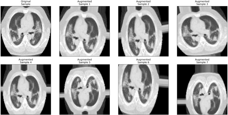
Another solution to the unavailability and diversity of data is to apply data augmentation (DA) techniques. DA helps to increase the size of the training set by producing more images from the original set by applying some image processing techniques (Salamon & Bello, 2017). On the other hand, DA can help to avoid the overfitting problem by providing more training examples so that the network can learn and extract important features only (Shorten & Khoshgoftaar, 2019). DA can be achieved by manipulating the original image to get a new image that is quite different from its source by using several methods (Başaran, Cömert, & Çelik, 2020) such as cropping, zooming, shearing, rotating, flipping, and changing the brightness.
To crop an image means to take only a selected part of the image and neglect the remaining parts. Zooming in (or out) means to either make the image closer (or farther away). Shearing an image is to transfer one part of an image in a direction and the other part in the opposite direction. Rotating an image means changing the angle of the image around its center either in a clockwise or a counterclockwise direction. Flipping has a mirror-like effect, which means that the image is changed either vertically, horizontally, or both as if in a mirror. Brightness affects the light amount in an image so that the image can be darker or lighter. Fig. 4 shows the result of applying different augmentation methods on a sample CT chest image.
Fig. 4.
Data Augmentation Graphical Illustration using a CT Image.
3.5. Harris Hawks Optimization (HHO)
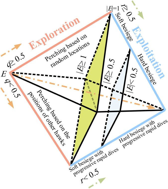
Harris Hawks Optimization (HHO) was introduced by Heidari et al. (2019) as a population-based swarm algorithm for solving different optimization problems. This algorithm mathematically mimics the feeding behavior of the Harris hawks in that they collaborate to explore, hunt, surprise, and chase preys (e.g. rabbits). Similar to most of the optimization algorithms, HHO has both the exploration and exploitation phases. The phases are summarized in Fig. 5.
Fig. 5.
Graphical Summary on the Harris Hawks Optimization (HHO) Phases (Heidari et al., 2019).
Exploration Phase: During the exploration phase, the hawks patiently search and explore for the desired prey after perching on some random locations. There are two different followed strategies by the hawks where each of them has a probability of the half for selection.
For the first strategy , the hawks can observe the prey based on the positions of other members in the hunting swarm. On the other hand, the second strategy means that hawks can perch randomly on the trees to explore the entire search area. These two states can be expressed by Eq. (10).
| (10) |
where represents the position vector update of the hawks in the next iteration , represents the position vector of the hawks in the current iteration , represents the position of a random hawk, represents the position of the prey, , , , , and represent random numbers in the range , and represent the lower and upper bounds of the variables, and is the average of the positions of the hawks calculated using Eq. (11).
| (11) |
where is the current position of hawk , and is the population size (i.e. total number of hawks in the swarm).
Transition from Exploration to Exploitation Phase: HHO has an additional phase, namely “transition from exploration to exploitation”, in which the hawks calculate the energy of the prey. This phase is the intermediate state between exploration and exploitation in which the prey tries to escape from the hawks’ attacks. As the prey is running away, its escaping energy is reduced based on Eq. (12).
| (12) |
where is the initial escaping energy of the prey, and is the total number of iterations of the algorithm. The value of the escaping energy lies in the interval . The values of outside this interval indicate that the exploration phase has not terminated yet. The exploration occurs when while the exploitation occurs when .
Exploitation Phase: In the exploitation phase, the hawks move based on the calculated energy to surround the rabbit from different directions. The positions of the hawks in nature are mapped to the desired possible solutions and the best position belongs to the hawk with the closest position to the prey. This phase contains two basic behaviors, namely attacking hawks and running away from the prey. The hawks attack their victims in a behavior called “surprise pounce”. The attacking of the hawks has four different techniques, depending on specific conditions, which are (1) soft besiege, (2) soft besiege with progressive rapid dives, (3) hard besiege, and (4) hard besiege with progressive rapid dives.
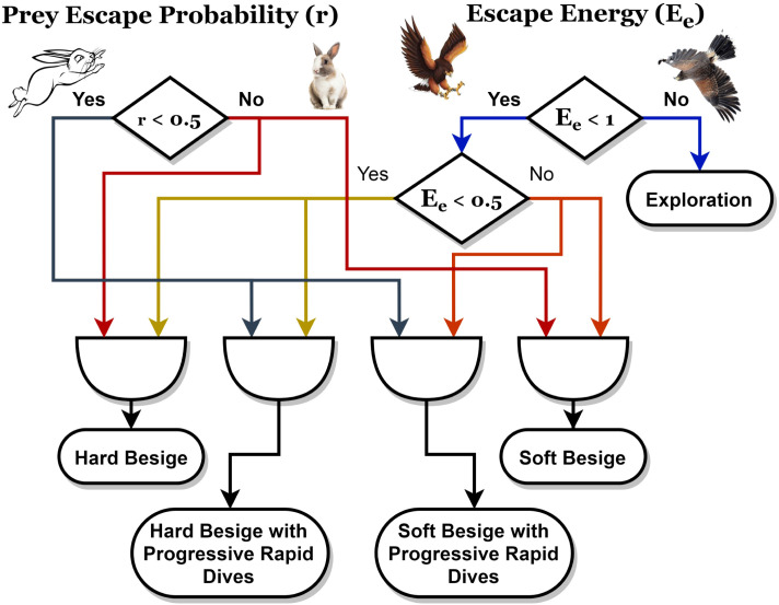
The choice between the different techniques depends on two parameters, namely the probability of escape of the prey and the escaping energy of the prey . is a probability that lies in the range from to . However, we have already mentioned that lies between and . The possibilities of and divided as shown in Fig. 6.
Fig. 6.
The Different HHO Possibilities in the Exploitation Phase.
If , this means that the prey has more chance of escape; otherwise, the prey will not be able to escape. means the prey has insufficient energy to escape; otherwise, the prey has enough energy. is used to specify whether the surrounding is hard or soft, while is used to choose between rapid and normal steps.
First Technique: Soft Besiege: This technique is applied when and . In this case, the prey is not able to escape and the hawks apply soft surroundings as shown in Eq. (13).
| (13) |
where is the distance between the prey and the current hawk in iteration (i.e. , and is the amount of escape made by the prey and is calculated using Eq. (14) where is a random value between to .
| (14) |
Second Technique: Hard Besiege: This technique is applied when and . In this case, the prey is drained that the hawks need no power to catch them as shown in Eq. (15).
| (15) |
Third Technique: Soft Besiege with Progressive Rapid Dives: This technique is applied when and . In this case, the prey still has some energy to run away and the hawks use soft besiege. In this situation, the hawks react in a way such that they choose the most suitable steps towards the prey. They calculate the consequence of their possible next step towards the prey. If this step is useful, then they use Eq. (16) to update their current position. Otherwise, they apply the levy flight (LF) technique to approach the prey in rapid dives based on Eq. (17).
| (16) |
| (17) |
where is the search space dimensions, is a random vector of size , and is levy flight function expressed by Eq. (18).
| (18) |
where and are random values from to , and is a constant value of 1.5. is calculated using Eq. (19).
| (19) |
The final equation for the position update in case of soft besiege with progressive rapid dives is Eq. (20).
| (20) |
where is a fitness function.
Fourth Technique: Hard Besiege with Progressive Rapid Dives: This technique is applied when and . In this case, the prey has no energy to run away and the hawks use hard-besiege. The hawks use the same technique used in soft besiege with progressive rapid dives situation. However, they minimize the gap between their average location and the location of the prey. The used equation for updating the position is shown in Eq. (21).
| (21) |
where and are calculated from Eqs. (22), (23) respectively.
| (22) |
| (23) |
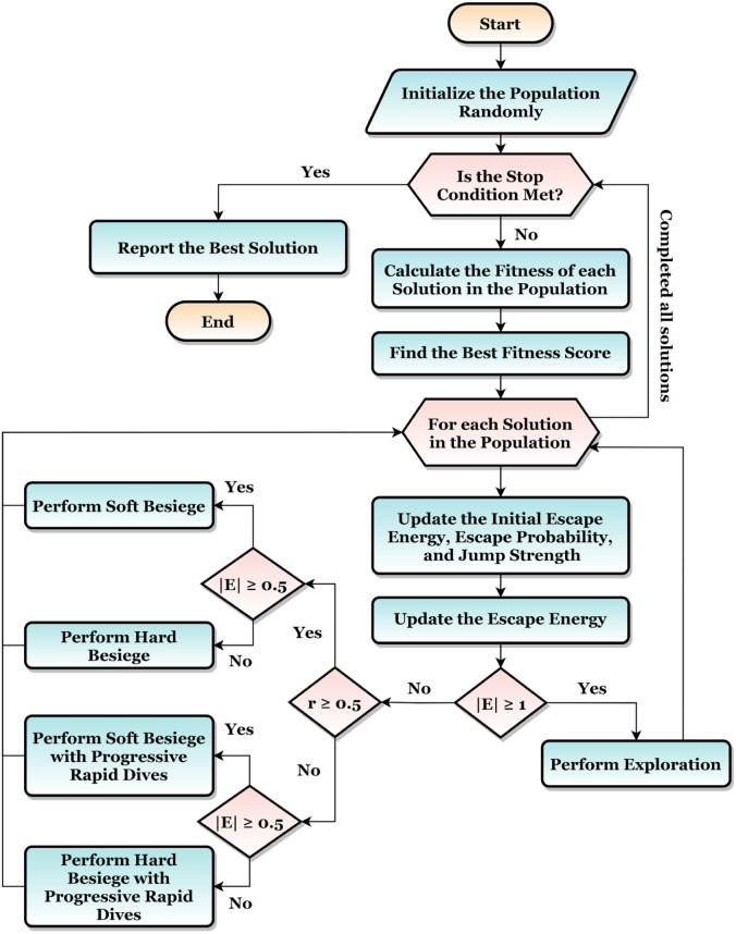
The overall flow of the HHO is summarized in Fig. 7.
Fig. 7.
The HHO Overall Flow Summarization.
4. CovH2SD: A hybrid harris hawks optimization deep learning approach
The main motivation towards the evolution of our proposed CovH2SD approach is to diagnose the patients that have COVID-19 or not. Time is a critical issue during the investigation of the COVID-19, as one patient can cause infection to his surroundings. So, early detection and isolation of patients can help to stop the spread of the virus.
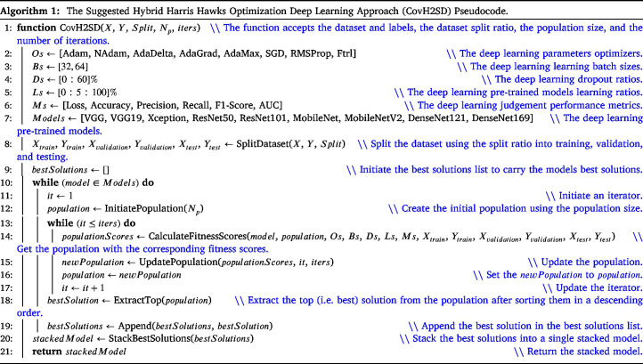
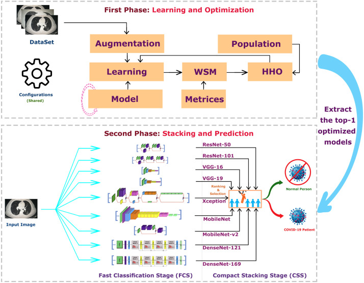
CovH2SD is a hybrid approach based on the idea of stacking different CNN models as shown in Fig. 8. The transfer learning approach is used as there are only limited accuracy datasets in this topic compared to others. The suggested approach uses nine different models. They are ResNet50 and ResNet101 (He et al., 2016), VGG16 and VGG19 (Simonyan & Zisserman, 2014), Xception (Chollet, 2017), MobileNet (Howard et al., 2017), MobileNetV2 (Sandler et al., 2018), DenseNet121, and DenseNet169 (Huang et al., 2017). We trained and fine-tuned these models with the COVID-19 CT dataset. The HHO algorithm is injected into the learning process. After the learning process is completed, we used a stacking mechanism to conduct a new model that is more accurate and robust than the individual ones. Algorithm 1 shows the optimization and learning internal steps of the CovH2SD approach.
Fig. 8.
CovH2SD: A Hybrid Harris Hawks Optimization Deep Learning Approach.
Algorithm 1 outlines the major phases of the suggested approach. It accepts the dataset and the corresponding categories (i.e. labels) , the dataset split ratio , the population size , and the number of iterations . It uses the Harris Hawks Optimization (HHO) to optimize the hyperparameters during the iterations. The hyperparameters that are required to be optimized are (1) the parameters optimizers , (2) the deep learning pre-trained models learning ratio , (3) the dropout ratio , and (4) the learning batch size . Simply, the HHO is used to answer the following question “For each model, what is the best hyperparameters combination that leads to the best performance after completing the iterations?”.
Adam, NAdam, AdaDelta, AdaGrad, AdaMax, SGD, RMSProp, and Ftrl are the used parameters (i.e. weights) optimizers, are the used batch sizes, is the range of the dropouts, and is the range of the learning ratios. VGG, VGG19, Xception, ResNet50, ResNet101, MobileNet, MobileNetV2, DenseNet121, and DenseNet169 are the pre-trained CNN models that are used in the current study.
The dataset is split into training, testing, and validation using the ratio. The training portion is used in the learning process, the validation is used to judge the model performance during the learning process, and the testing portion is used to evaluate the model performance after finishing its learning process. A loop is applied on each model from the used pre-trained CNN models. For each model, the following steps are followed:
(1) Initiate the Population: The initial population is created. The number of solutions is defined by and the size of a single solution is as we have four hyperparameters that are required to be optimized. Hence, the population is a matrix with a size of . Each value is random from to . These values will be mapped in the next step into the corresponding hyperparameters.
(2) Calculate Fitness Scores: For each of the solutions, the fitness scores are calculated. The implementation of this step is shown in Algorithm 2. The population, current model, hyperparameters, and data are sent as inputs to that function.
For each of the solutions, the solution is first mapped to hyperparameters. They are injected into the learning process. The pre-trained CNN model is trained for a set of epochs on these hyperparameters. After learning, the performance is calculated and appended in the population scores list. The used performance metrics are Loss, Accuracy, Precision, Recall, F1-Score, and Area Under Curve (AUC). Accuracy is the ratio between the total number of right predictions and the total number of predictions made by the model as shown in Eq. (24).
| (24) |
where TP, TN, FP, FN are true positive, true negative, false positive, and false negative respectively. TP is the case when the forecasts of the data are positive, and the results of the model are also positive. TN is the case when the forecasts of the data are negative, and the results of the model are also negative. FP is the case when the forecasts of the data are negative, and the results of the model are positive. FN is the case when the forecasts of the data are positive, and the results of the model are negative.
Precision is the ratio between the total number of true positive predictions and the total number of positive predictions made by the model as shown in Eq. (25). The recall is the ratio between the total number of true positive predictions and the total number of true positive and false negative predictions made by the model as shown in Eq. (26). F1-score is the harmonic mean of precision and recall as shown in Eq. (27) (Balaha, Ali, Saraya, & Badawy, 2021).
| (25) |
| (26) |
| (27) |
As we are dealing with six metrics, it is required to map them into a single fitness score. The Weighted Sum Method (WSM) is used. It is a method that takes a percentage from each value and sums them together into a single value. The percentages of them are equalized for all unless the loss as shown in Eq. (28). It is worth mentioning that, the reciprocal of the loss is used as it is required to minimize it while maximizing the rest.
| (28) |
(3) Update the Population: After calculating the fitness scores for the population, they should be updated for the next iteration. The HHO is used in this step. The working mechanism of the HHO is discussed in the previous section. It is worth mentioning that the current study works with a maximization problem while the original HHO paper worked with a minimization problem. The only change will be in Eq. (20) and Eq. (21). For maximization problems, the is replaced with . Steps and will be repeated until the completion of the HHO optimization iterations.
(4) Stack Best Solutions: After extracting the best combination for each model of the nine tuned models, they beside their best combinations are stacked into a single model. They will be used in future predictions and production phases.
In the production phase, every input image is duplicated nine times and presented as an input to each of the chosen nine CNN architectures. Every network extracts the features from the input image and these features are used in the recognition process. The input image propagates through the different layers (i.e. convolution, pooling, and FC layers) of the different networks. The output of each model represents the probability of each class of our binary classification model and contributes as an input to the stacked model. CovH2SD uses a novel mechanism for ranking different stacking configurations by mapping them into a proposed Quality Space (QS). QS is a Q-dimensional space, where represents the number of all possible configurations of stacking. The rank of each configuration is calculated. This rank is represented by a point in the quality space. The algorithm switches automatically between the different stacked models. The models with the most significant ranks are used to create the final classification model that will identify new individuals as patients or normal.
5. Experiments, results, and discussion
The current section begins by presenting the used dataset, the experimental configurations used in the learning and optimization, discusses the applied experiments, and reports the corresponding results. The section ends by constructing a comparative study between the current study and other state-of-the-art studies.
5.1. Dataset
The dataset is collected from three sources. The first source is “COVID-CT-Dataset: A CT Scan Dataset about COVID-19” (Zhao, Zhang, He, & Xie, 2020) and can be accessed from https://www.kaggle.com/luisblanche/covidct. It consisted of and images for the COVID-19 and non-COVID-19 cases respectively. The second source is “CT Scans for COVID-19 Classification” (Ning et al., 2020) and can be accessed from https://www.kaggle.com/azaemon/preprocessed-ct-scans-for-covid19. It consisted of 4,001 and 9,979 images for the COVID-19 and non-COVID-19 cases respectively. The third source is “COVID-CTset” (Rahimzadeh, Attar, & Sakhaei, 2020) and can be accessed from https://github.com/mr7495/COVID-CTset. It consisted of 15,589 and 48,260 images for the COVID-19 and non-COVID-19 cases respectively.
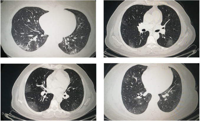
The images are combines and filtered manually. The resultant total number of images is 15,535 CT images with 5,159 images of confirmed positive COVID-19 cases and 10,376 images of normal (non-COVID-19) cases. Samples of the CT images with COVID-19 are shown in Fig. 9. Data augmentation is applied to increase the diversity of the dataset using the configurations in Table 2.
Fig. 9.
Samples of the CT Images with COVID-19.
Table 2.
Data augmentation configurations.
| Method | Range |
|---|---|
| Rotation | |
| Width Shift Range | |
| Height Shift Range | |
| Shear Range | |
| Zoom Range | |
| Horizontal Flipping | True |
| Vertical Flipping | True |
5.2. Experiments and discussion
Table 3 presents the configurations used in the experiments.
Table 3.
The used experiments configurations.
| Method | Range |
|---|---|
| Dataset | Collected from 3 sources. |
| Categories | “COVID-19” and “non-COVID-19”. |
| Split Ratio | 90% to 10% |
| Dataset Size | 15,535 |
| Data Augmentation | Yes (Table 2) |
| Pre-trained Models | VGG16, VGG19, ResNet50, ResNet101, DenseNet121, DenseNet169, MobileNet, MobileNetV2, and Xception |
| Pre-trained Parameters Initializers | ImageNet |
| Output Activation Function | SoftMax |
| Number of Epochs | 64 |
| Parameters optimizers | Adam, NAdam, AdaGrad, AdaDelta, AdaMax, RMSProp, Ftrl, and SGD |
| TL learn ratios | |
| Batch sizes | 32 and 64 |
| Dropout ratios | |
| Performance Metrics | Loss, Accuracy, Precision, F1-score, AUC, and Recall |
| Number of HHO Iterations | 15 |
| Population Size | 10 |
| Learning and Optimization Environment | Google Colab (Intel(R) Xeon(R) CPU @ 2.00 GHz, Tesla T4 16 GB GPU with CUDA v.11.2, and 12 GB RAM) |
| Programming Language | Python |
| Python Packages | Tensorflow, Keras, NumPy, OpenCV, Pandas, and Matplotlib |
VGG16: Table 4 reports the top-1 combination in each hyperparameters optimization iteration in the optimization iterations for the VGG16 pre-trained CNN model with the corresponding performance metrics. Each iteration has as the population size where each solution is trained for epochs.
Table 4.
Top-1 combinations for the VGG16 in the 15 optimization iterations.
| # | Parameters optimizer | Batch size | Dropout ratio | TL learn ratio | Loss | Accuracy | F1 | Precision | Recall | AUC | WSM |
|---|---|---|---|---|---|---|---|---|---|---|---|
| 1 | SGD | 32 | 0.57 | 80% | 0.0716 | 97.21% | 97.21% | 97.21% | 97.21% | 0.9966 | 95.48% |
| 2 | SGD | 32 | 0.56 | 80% | 0.0952 | 96.63% | 96.63% | 96.63% | 96.63% | 0.9946 | 94.74% |
| 3 | AdaGrad | 32 | 0.21 | 30% | 0.2933 | 91.25% | 91.25% | 91.25% | 91.25% | 0.9674 | 89.14% |
| 4 | SGD | 32 | 0.58 | 80% | 0.0584 | 98.08% | 98.08% | 98.08% | 98.08% | 0.9967 | 96.48% |
| 5 | AdaGrad | 32 | 0.19 | 25% | 0.1302 | 95.57% | 95.58% | 95.57% | 95.57% | 0.9897 | 93.57% |
| 6 | SGD | 32 | 0.58 | 80% | 0.0394 | 98.61% | 98.61% | 98.61% | 98.61% | 0.9980 | 97.41% |
| 7 | SGD | 32 | 0.58 | 80% | 0.0263 | 99.13% | 99.13% | 99.13% | 99.13% | 0.9991 | 98.55% |
| 8 | SGD | 32 | 0.58 | 80% | 0.0252 | 99.23% | 99.23% | 99.23% | 99.23% | 0.9988 | 98.73% |
| 9 | SGD | 32 | 0.58 | 80% | 0.0221 | 99.23% | 99.23% | 99.23% | 99.23% | 0.9993 | 99.02% |
| 10 | SGD | 32 | 0.58 | 80% | 0.0314 | 98.99% | 98.99% | 98.99% | 98.99% | 0.9995 | 98.11% |
| 11 | SGD | 32 | 0.58 | 80% | 0.0324 | 98.94% | 98.94% | 98.94% | 98.94% | 0.9986 | 98.01% |
| 12 | SGD | 32 | 0.58 | 80% | 0.0226 | 99.28% | 99.28% | 99.28% | 99.28% | 0.9993 | 99.01% |
| 13 | SGD | 32 | 0.58 | 80% | 0.0247 | 99.09% | 99.09% | 99.09% | 99.09% | 0.9988 | 98.63% |
| 14 | SGD | 32 | 0.58 | 80% | 0.0251 | 99.09% | 99.09% | 99.09% | 99.09% | 0.9988 | 98.60% |
| 15 | SGD | 32 | 0.58 | 80% | 0.0292 | 98.85% | 98.85% | 98.85% | 98.85% | 0.9987 | 98.09% |
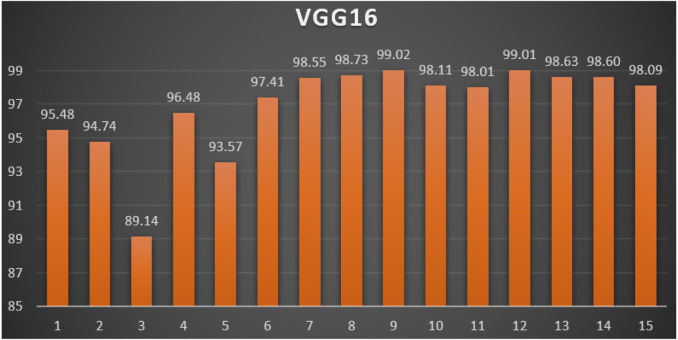
From Table 4, the SGD was the best parameters optimizer in iterations. The batch size with a value of was the best in iterations. The dropout ratio with a value of 58% was the best in iterations. The learning ratio with a value of 80% was the best in iterations. The best achieved distinctive metrics for the loss, accuracy, F1, precision, recall, AUC, and WSM were 0.0221, 99.28%, 99.28%, 99.28%, 99.28%, 0.9995, and 99.02% respectively. The best achieved combination was in iteration number where its metrics were 0.0221, 99.23%, 99.23%, 99.23%, 99.23%, 0.9993, and 99.02% respectively. All of the WSM scores were above 89%. Fig. 10 shows the WSM curve for the iterations.
Fig. 10.
The WSM Curve for the VGG16.
VGG19: Table 5 reports the top-1 combination in each hyperparameters optimization iteration in the optimization iterations for the VGG19 pre-trained CNN model with the corresponding performance metrics. Each iteration has as the population size where each solution is trained for epochs.
Table 5.
Top-1 combinations for the VGG19 in the 15 optimization iterations.
| # | Parameters optimizer | Batch size | Dropout ratio | TL learn ratio | Loss | Accuracy | F1 | Precision | Recall | AUC | WSM |
|---|---|---|---|---|---|---|---|---|---|---|---|
| 1 | SGD | 32 | 0.57 | 80% | 0.0707 | 97.55% | 97.55% | 97.55% | 97.55% | 0.9951 | 95.82% |
| 2 | SGD | 32 | 0.54 | 75% | 0.2442 | 93.94% | 93.94% | 93.94% | 93.94% | 0.9750 | 91.80% |
| 3 | SGD | 32 | 0.55 | 80% | 0.0696 | 97.02% | 97.02% | 97.02% | 97.02% | 0.9958 | 95.31% |
| 4 | NAdam | 32 | 0.14 | 15% | 0.2160 | 91.73% | 91.72% | 91.73% | 91.73% | 0.9755 | 89.66% |
| 5 | NAdam | 64 | 0.16 | 20% | 0.4726 | 87.88% | 87.88% | 87.88% | 87.88% | 0.9351 | 85.79% |
| 6 | AdaGrad | 32 | 0.27 | 25% | 0.2545 | 92.78% | 92.78% | 92.78% | 92.78% | 0.9718 | 90.66% |
| 7 | AdaGrad | 32 | 0.27 | 25% | 0.4300 | 90.00% | 89.99% | 90.00% | 90.00% | 0.9466 | 87.86% |
| 8 | SGD | 32 | 0.56 | 80% | 0.0737 | 97.55% | 97.55% | 97.55% | 97.55% | 0.9970 | 95.79% |
| 9 | SGD | 32 | 0.56 | 80% | 0.0364 | 98.46% | 98.46% | 98.46% | 98.46% | 0.9992 | 97.37% |
| 10 | SGD | 32 | 0.56 | 80% | 0.0375 | 98.80% | 98.80% | 98.80% | 98.80% | 0.9981 | 97.66% |
| 11 | SGD | 32 | 0.56 | 80% | 0.0359 | 98.70% | 98.70% | 98.70% | 98.70% | 0.9988 | 97.63% |
| 12 | SGD | 32 | 0.56 | 80% | 0.0319 | 98.75% | 98.75% | 98.75% | 98.75% | 0.9990 | 97.85% |
| 13 | SGD | 32 | 0.56 | 80% | 0.0310 | 98.89% | 98.89% | 98.89% | 98.89% | 0.9991 | 98.03% |
| 14 | SGD | 32 | 0.56 | 80% | 0.0202 | 99.33% | 99.33% | 99.33% | 99.33% | 0.9988 | 99.31% |
| 15 | SGD | 32 | 0.56 | 80% | 0.0212 | 99.09% | 99.09% | 99.09% | 99.09% | 0.9998 | 98.97% |
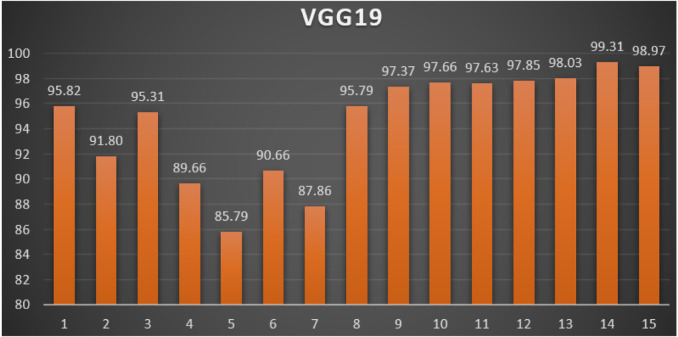
From Table 5, the SGD was the best parameters optimizer in iterations. The batch size with a value of was the best in iterations. The dropout ratio with a value of 56% was the best in iterations. The learning ratio with a value of 80% was the best in iterations. The best achieved distinctive metrics for the loss, accuracy, F1, precision, recall, AUC, and WSM were 0.0202, 99.33%, 99.33%, 99.33%, 99.33%, 0.9998, and 99.31% respectively. The best achieved combination was in iteration number where its metrics were 0.0202, 99.33%, 99.33%, 99.33%, 99.33%, 0.9998, and 99.31% respectively. All of the WSM scores were above 85%. Fig. 11 shows the WSM curve for the iterations.
Fig. 11.
The WSM Curve for the VGG19.
ResNet50: Table 6 reports the top-1 combination in each hyperparameters optimization iteration in the optimization iterations for the ResNet50 pre-trained CNN model with the corresponding performance metrics. Each iteration has as the population size where each solution is trained for epochs.
Table 6.
Top-1 combinations for the ResNet50 in the 15 optimization iterations.
| # | Parameters optimizer | Batch size | Dropout ratio | TL learn ratio | Loss | Accuracy | F1 | Precision | Recall | AUC | WSM |
|---|---|---|---|---|---|---|---|---|---|---|---|
| 1 | RMSProp | 64 | 0.54 | 70% | 0.5798 | 77.63% | 77.63% | 77.63% | 77.63% | 0.8617 | 75.78% |
| 2 | RMSProp | 64 | 0.54 | 70% | 0.6359 | 70.18% | 70.18% | 70.18% | 70.18% | 0.7713 | 68.50% |
| 3 | Adam | 32 | 0% | 0% | 1.6620 | 51.03% | 51.03% | 51.03% | 51.03% | 0.5533 | 49.79% |
| 4 | Adam | 32 | 0.01 | 0% | 2.0220 | 51.03% | 51.03% | 51.03% | 51.03% | 0.5442 | 49.78% |
| 5 | AdaGrad | 32 | 0.23 | 30% | 1.2469 | 51.03% | 51.03% | 51.03% | 51.03% | 0.6198 | 49.80% |
| 6 | SGD | 32 | 0.6 | 100% | 0.3560 | 92.11% | 92.11% | 92.11% | 92.11% | 0.9652 | 89.95% |
| 7 | SGD | 32 | 0.6 | 100% | 0.1996 | 94.81% | 94.80% | 94.81% | 94.81% | 0.9817 | 92.69% |
| 8 | SGD | 32 | 0.6 | 100% | 0.0531 | 98.36% | 98.36% | 98.36% | 98.36% | 0.9979 | 96.85% |
| 9 | SGD | 32 | 0.6 | 100% | 0.0648 | 97.79% | 97.79% | 97.79% | 97.79% | 0.9971 | 96.11% |
| 10 | SGD | 32 | 0.6 | 100% | 0.0448 | 98.41% | 98.41% | 98.41% | 98.41% | 0.9979 | 97.07% |
| 11 | SGD | 32 | 0.6 | 100% | 0.0479 | 98.80% | 98.80% | 98.80% | 98.80% | 0.9970 | 97.37% |
| 12 | SGD | 32 | 0.6 | 100% | 0.0394 | 98.85% | 98.85% | 98.85% | 98.85% | 0.9988 | 97.64% |
| 13 | SGD | 32 | 0.6 | 100% | 0.0598 | 98.27% | 98.27% | 98.27% | 98.27% | 0.9959 | 96.65% |
| 14 | SGD | 32 | 0.6 | 100% | 0.0666 | 97.74% | 97.74% | 97.74% | 97.74% | 0.9972 | 96.05% |
| 15 | SGD | 32 | 0.6 | 100% | 0.0707 | 98.17% | 98.17% | 98.17% | 98.17% | 0.9957 | 96.43% |
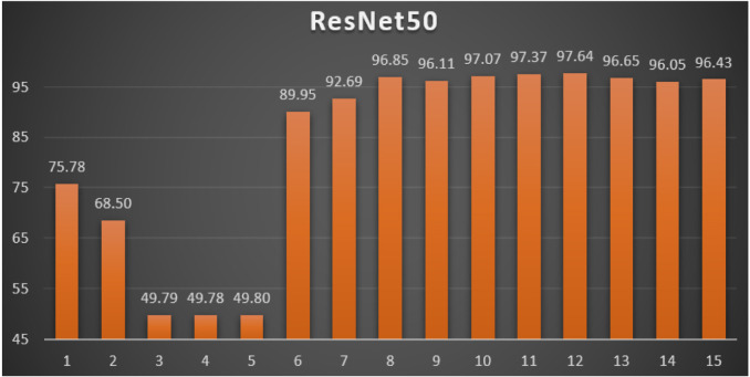
From Table 6, the SGD was the best parameters optimizer in iterations. The batch size with a value of was the best in iterations. The dropout ratio with a value of 60% was the best in iterations. The learning ratio with a value of 100% was the best in iterations. The best achieved distinctive metrics for the loss, accuracy, F1, precision, recall, AUC, and WSM were 0.0394, 98.85%, 98.85%, 98.85%, 98.85%, 0.9988, and 97.64% respectively. The best achieved combination was in iteration number where its metrics were 0.0394, 98.85%, 98.85%, 98.85%, 98.85%, 0.9988, and 97.64% respectively. All of the WSM scores were above 49%. Fig. 12 shows the WSM curve for the iterations.
Fig. 12.
The WSM Curve for the ResNet50.
ResNet101: Table 7 reports the top-1 combination in each hyperparameters optimization iteration in the optimization iterations for the ResNet101 pre-trained CNN model with the corresponding performance metrics. Each iteration has as the population size where each solution is trained for epochs.
Table 7.
Top-1 combinations for the ResNet101 in the 15 optimization iterations.
| # | Parameters optimizer | Batch size | Dropout ratio | TL learn ratio | Loss | Accuracy | F1 | Precision | Recall | AUC | WSM |
|---|---|---|---|---|---|---|---|---|---|---|---|
| 1 | NAdam | 32 | 0.17 | 25% | 0.7040 | 51.03% | 51.03% | 51.03% | 51.03% | 0.6038 | 49.83% |
| 2 | NAdam | 32 | 0.14 | 20% | 0.7079 | 52.91% | 52.92% | 52.91% | 52.91% | 0.5222 | 51.66% |
| 3 | NAdam | 32 | 0.09 | 10% | 0.8788 | 51.03% | 51.03% | 51.03% | 51.03% | 0.6062 | 49.81% |
| 4 | Ftrl | 64 | 0.6 | 100% | 0.6932 | 48.97% | 48.97% | 48.97% | 48.97% | 0.5000 | 47.82% |
| 5 | SGD | 64 | 0.6 | 100% | 0.1300 | 96.87% | 96.88% | 96.87% | 96.87% | 0.9884 | 94.84% |
| 6 | SGD | 64 | 0.6 | 100% | 0.0928 | 97.55% | 97.55% | 97.55% | 97.55% | 0.9921 | 95.65% |
| 7 | SGD | 64 | 0.6 | 100% | 0.0703 | 98.03% | 98.03% | 98.03% | 98.03% | 0.9950 | 96.29% |
| 8 | SGD | 64 | 0.6 | 100% | 0.0966 | 97.88% | 97.88% | 97.88% | 97.88% | 0.9915 | 95.95% |
| 9 | SGD | 64 | 0.6 | 100% | 0.0610 | 98.27% | 98.27% | 98.27% | 98.27% | 0.9963 | 96.63% |
| 10 | SGD | 64 | 0.6 | 100% | 0.0774 | 97.84% | 97.84% | 97.84% | 97.84% | 0.9957 | 96.04% |
| 11 | SGD | 64 | 0.6 | 100% | 0.1095 | 97.02% | 97.02% | 97.02% | 97.02% | 0.9916 | 95.05% |
| 12 | SGD | 64 | 0.6 | 100% | 0.0710 | 98.17% | 98.17% | 98.17% | 98.17% | 0.9957 | 96.42% |
| 13 | SGD | 64 | 0.6 | 100% | 0.0577 | 98.22% | 98.22% | 98.22% | 98.22% | 0.9974 | 96.63% |
| 14 | SGD | 64 | 0.6 | 100% | 0.1160 | 96.97% | 96.97% | 96.97% | 96.97% | 0.9908 | 94.98% |
| 15 | SGD | 64 | 0.6 | 100% | 0.0994 | 97.88% | 97.88% | 97.88% | 97.88% | 0.9937 | 95.94% |
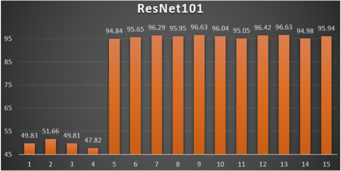
From Table 7, the SGD was the best parameters optimizer in iterations. The batch size with a value of was the best in iterations. The dropout ratio with a value of 60% was the best in iterations. The learning ratio with a value of 100% was the best in iterations. The best achieved distinctive metrics for the loss, accuracy, F1, precision, recall, AUC, and WSM were 0.0577, 98.22%, 98.22%, 98.22%, 98.22%, 0.9974, and 96.63% respectively. The last best achieved combination was in iteration number where its metrics were 0.0577, 98.27%, 98.27%, 98.27%, 98.27%, 0.9974, and 96.63% respectively. All of the WSM scores were above 89%. Fig. 13 shows the WSM curve for the iterations.
Fig. 13.
The WSM Curve for the ResNet101.
DenseNet121: Table 8 reports the top-1 combination in each hyperparameters optimization iteration in the optimization iterations for the DenseNet121 pre-trained CNN model with the corresponding performance metrics. Each iteration has as the population size where each solution is trained for epochs.
Table 8.
Top-1 combinations for the DenseNet121 in the 15 optimization iterations.
| # | Parameters optimizer | Batch size | Dropout ratio | TL learn ratio | Loss | Accuracy | F1 | Precision | Recall | AUC | WSM |
|---|---|---|---|---|---|---|---|---|---|---|---|
| 1 | NAdam | 32 | 0.12 | 20% | 23.631 | 51.32% | 51.33% | 51.32% | 51.32% | 0.5133 | 50.04% |
| 2 | NAdam | 64 | 0.15 | 25% | 16.683 | 51.13% | 51.14% | 51.13% | 51.13% | 0.5173 | 49.86% |
| 3 | AdaMax | 32 | 0.35 | 60% | 11.823 | 64.17% | 64.17% | 64.17% | 64.17% | 0.6532 | 62.57% |
| 4 | RMSProp | 64 | 0.44 | 80% | 13.235 | 57.09% | 57.10% | 57.09% | 57.09% | 0.5747 | 55.67% |
| 5 | RMSProp | 64 | 0.44 | 80% | 89.372 | 68.73% | 68.74% | 68.73% | 68.73% | 0.7027 | 67.02% |
| 6 | RMSProp | 32 | 0.39 | 70% | 2.0622 | 82.20% | 82.20% | 82.20% | 82.20% | 0.8562 | 80.17% |
| 7 | RMSProp | 64 | 0.38 | 70% | 5.9464 | 78.11% | 78.11% | 78.11% | 78.11% | 0.7976 | 76.17% |
| 8 | RMSProp | 64 | 0.38 | 70% | 32.481 | 80.13% | 80.14% | 80.13% | 80.13% | 0.8072 | 78.13% |
| 9 | RMSProp | 32 | 0.4 | 70% | 14.187 | 79.08% | 79.07% | 79.08% | 79.08% | 0.8099 | 77.10% |
| 10 | RMSProp | 32 | 0.39 | 70% | 3.9436 | 80.86% | 80.86% | 80.86% | 80.86% | 0.8297 | 78.85% |
| 11 | RMSProp | 32 | 0.39 | 70% | 3.6292 | 83.93% | 83.94% | 83.93% | 83.93% | 0.8629 | 81.85% |
| 12 | RMSProp | 32 | 0.41 | 75% | 0.6732 | 90.14% | 90.14% | 90.14% | 90.14% | 0.9487 | 87.96% |
| 13 | RMSProp | 32 | 0.41 | 75% | 2.7017 | 86.58% | 86.58% | 86.58% | 86.58% | 0.8917 | 84.44% |
| 14 | RMSProp | 64 | 0.38 | 70% | 13.832 | 81.39% | 81.38% | 81.39% | 81.39% | 0.8200 | 79.35% |
| 15 | RMSProp | 32 | 0.41 | 75% | 7.2526 | 76.67% | 76.68% | 76.67% | 76.67% | 0.7983 | 74.76% |
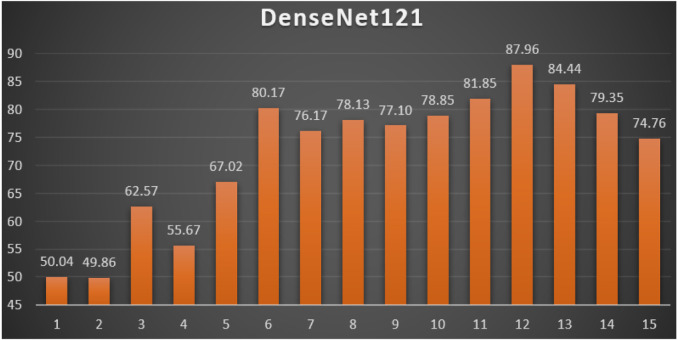
From Table 8, the RMSProp was the best parameters optimizer in iterations. The batch size with a value of was the best in iterations. The dropout ratios with values of 38%, 39%, and 41% were the best in iterations. The learning ratio with a value of 70% was the best in iterations. The best achieved distinctive metrics for the loss, accuracy, F1, precision, recall, AUC, and WSM were 0.6732, 90.14%, 90.14%, 90.14%, 90.14%, 0.9487, and 87.96% respectively. The best achieved combination was in iteration number where its metrics were 0.6732, 90.14%, 90.14%, 90.14%, 90.14%, 0.9487, and 87.96% respectively. All of the WSM scores were above 49%. Fig. 14 shows the WSM curve for the iterations.
Fig. 14.
The WSM Curve for the DenseNet121.
DenseNet169: Table 9 reports the top-1 combination in each hyperparameters optimization iteration in the optimization iterations for the DenseNet169 pre-trained CNN model with the corresponding performance metrics. Each iteration has as the population size where each solution is trained for epochs.
Table 9.
Top-1 combinations for the DenseNet169 in the 15 optimization iterations.
| # | Parameters optimizer | Batch size | Dropout ratio | TL learn ratio | Loss | Accuracy | F1 | Precision | Recall | AUC | WSM |
|---|---|---|---|---|---|---|---|---|---|---|---|
| 1 | AdaMax | 32 | 0.37 | 50% | 1.1045 | 78.11% | 78.10% | 78.11% | 78.11% | 0.8572 | 76.20% |
| 2 | RMSProp | 64 | 0.5 | 70% | 15.632 | 82.06% | 82.06% | 82.06% | 82.06% | 0.8228 | 80.01% |
| 3 | AdaMax | 32 | 0.36 | 50% | 1.7170 | 85.67% | 85.66% | 85.67% | 85.67% | 0.8845 | 83.55% |
| 4 | AdaMax | 32 | 0.36 | 50% | 1.9082 | 88.02% | 88.02% | 88.02% | 88.02% | 0.9028 | 85.85% |
| 5 | AdaMax | 32 | 0.36 | 50% | 1.6761 | 88.89% | 88.89% | 88.89% | 88.89% | 0.9100 | 86.70% |
| 6 | AdaMax | 32 | 0.36 | 50% | 1.7754 | 88.02% | 88.02% | 88.02% | 88.02% | 0.9028 | 85.85% |
| 7 | AdaMax | 32 | 0.36 | 50% | 1.1883 | 89.71% | 89.70% | 89.71% | 89.71% | 0.9261 | 87.50% |
| 8 | AdaMax | 32 | 0.36 | 50% | 1.2521 | 88.07% | 88.06% | 88.07% | 88.07% | 0.9117 | 85.91% |
| 9 | AdaMax | 32 | 0.36 | 50% | 1.7210 | 88.84% | 88.84% | 88.84% | 88.84% | 0.9103 | 86.65% |
| 10 | AdaMax | 32 | 0.36 | 50% | 1.1751 | 88.12% | 88.11% | 88.12% | 88.12% | 0.9153 | 85.95% |
| 11 | AdaMax | 32 | 0.36 | 50% | 1.0352 | 89.56% | 89.56% | 89.56% | 89.56% | 0.9290 | 87.37% |
| 12 | AdaMax | 32 | 0.36 | 50% | 1.6333 | 87.73% | 87.73% | 87.73% | 87.73% | 0.9005 | 85.57% |
| 13 | AdaMax | 32 | 0.36 | 50% | 1.3847 | 87.01% | 87.01% | 87.01% | 87.01% | 0.9043 | 84.87% |
| 14 | AdaMax | 32 | 0.36 | 50% | 1.1712 | 90.76% | 90.76% | 90.76% | 90.76% | 0.9294 | 88.54% |
| 15 | AdaMax | 32 | 0.36 | 50% | 1.0113 | 89.66% | 89.66% | 89.66% | 89.66% | 0.9244 | 87.47% |
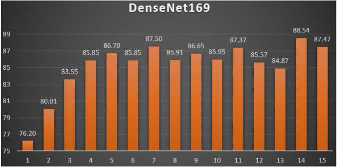
From Table 9, the AdaMax was the best parameters optimizer in iterations. The batch size with a value of was the best in iterations. The dropout ratio with a value of 36% was the best in iterations. The learning ratio with a value of 50% was the best in iterations. The best achieved distinctive metrics for the loss, accuracy, F1, precision, recall, AUC, and WSM were 1.0113, 90.76%, 90.76%, 90.76%, 90.76%, 0.9294, and 88.54% respectively. The best achieved combination was in iteration number where its metrics were 1.1712, 90.76%, 90.76%, 90.76%, 90.76%, 0.9294, and 88.54% respectively. All of the WSM scores were above 76%. Fig. 15 shows the WSM curve for the iterations.
Fig. 15.
The WSM Curve for the DenseNet169.
MobileNet: Table 10 reports the top-1 combination in each hyperparameters optimization iteration in the optimization iterations for the MobileNet pre-trained CNN model with the corresponding performance metrics. Each iteration has as the population size where each solution is trained for epochs.
Table 10.
Top-1 combinations for the MobileNet in the 15 optimization iterations.
| # | Parameters optimizer | Batch size | Dropout ratio | TL learn ratio | Loss | Accuracy | F1 | Precision | Recall | AUC | WSM |
|---|---|---|---|---|---|---|---|---|---|---|---|
| 1 | AdaDelta | 64 | 0.59 | 90% | 0.6718 | 79.70% | 79.70% | 79.70% | 79.70% | 0.8643 | 77.78% |
| 2 | AdaMax | 32 | 0.6 | 100% | 0.5892 | 90.57% | 90.57% | 90.57% | 90.57% | 0.9482 | 88.39% |
| 3 | AdaMax | 32 | 0.6 | 100% | 0.6249 | 90.96% | 90.96% | 90.96% | 90.96% | 0.9476 | 88.76% |
| 4 | AdaGrad | 64 | 0.31 | 50% | 4.1396 | 54.35% | 54.36% | 54.35% | 54.35% | 0.5796 | 53.01% |
| 5 | SGD | 64 | 0.6 | 100% | 0.1050 | 96.73% | 96.73% | 96.73% | 96.73% | 0.9928 | 94.79% |
| 6 | SGD | 64 | 0.6 | 100% | 0.1323 | 95.96% | 95.96% | 95.96% | 95.96% | 0.9901 | 93.94% |
| 7 | SGD | 64 | 0.6 | 100% | 0.0807 | 97.69% | 97.69% | 97.69% | 97.69% | 0.9950 | 95.87% |
| 8 | SGD | 64 | 0.6 | 100% | 0.0538 | 98.08% | 98.08% | 98.08% | 98.08% | 0.9965 | 96.55% |
| 9 | SGD | 64 | 0.6 | 100% | 0.0433 | 98.75% | 98.75% | 98.75% | 98.75% | 0.9983 | 97.44% |
| 10 | SGD | 64 | 0.6 | 100% | 0.0440 | 98.46% | 98.46% | 98.46% | 98.46% | 0.9964 | 97.13% |
| 11 | SGD | 64 | 0.6 | 100% | 0.1060 | 97.26% | 97.26% | 97.26% | 97.26% | 0.9921 | 95.30% |
| 12 | SGD | 64 | 0.6 | 100% | 0.0610 | 98.17% | 98.17% | 98.17% | 98.17% | 0.9970 | 96.54% |
| 13 | SGD | 64 | 0.6 | 100% | 0.0535 | 98.27% | 98.27% | 98.27% | 98.27% | 0.9982 | 96.75% |
| 14 | SGD | 64 | 0.6 | 100% | 0.0524 | 98.36% | 98.37% | 98.36% | 98.36% | 0.9967 | 96.86% |
| 15 | SGD | 64 | 0.6 | 100% | 0.0413 | 98.51% | 98.51% | 98.51% | 98.51% | 0.9979 | 97.26% |
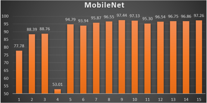
From Table 10, the SGD was the best parameters optimizer in iterations. The batch size with a value of was the best in iterations. The dropout ratio with a value of 60% was the best in iterations. The learning ratio with a value of 100% was the best in iterations. The best achieved distinctive metrics for the loss, accuracy, F1, precision, recall, AUC, and WSM were 0.0433, 98.75%, 98.75%, 98.75%, 98.75%, 0.9983, and 97.44% respectively. The best achieved combination was in iteration number where its metrics were 0.0433, 98.75%, 98.75%, 98.75%, 98.75%, 0.9983, and 97.44% respectively. All of the WSM scores were above 53%. Fig. 16 shows the WSM curve for the iterations.
Fig. 16.
The WSM Curve for the MobileNet.
MobileNetV2: Table 11 reports the top-1 combination in each hyperparameters optimization iteration in the optimization iterations for the MobileNetV2 pre-trained CNN model with the corresponding performance metrics. Each iteration has as the population size where each solution is trained for epochs.
Table 11.
Top-1 combinations for the MobileNetV2 in the 15 optimization iterations.
| # | Parameters optimizer | Batch size | Dropout ratio | TL learn ratio | Loss | Accuracy | F1 | Precision | Recall | AUC | WSM |
|---|---|---|---|---|---|---|---|---|---|---|---|
| 1 | AdaDelta | 32 | 0.28 | 0% | 0.7376 | 64.21% | 64.22% | 64.21% | 64.21% | 0.6683 | 62.68% |
| 2 | AdaDelta | 32 | 0.28 | 0% | 0.7386 | 64.41% | 64.41% | 64.41% | 64.41% | 0.6675 | 62.87% |
| 3 | AdaDelta | 32 | 0.28 | 0% | 0.7368 | 64.55% | 64.56% | 64.55% | 64.55% | 0.6690 | 63.01% |
| 4 | AdaDelta | 32 | 0.28 | 0% | 0.7388 | 64.17% | 64.17% | 64.17% | 64.17% | 0.6663 | 62.63% |
| 5 | AdaDelta | 32 | 0.28 | 0% | 0.7367 | 64.60% | 64.60% | 64.60% | 64.60% | 0.6687 | 63.05% |
| 6 | AdaDelta | 32 | 0.28 | 0% | 0.7360 | 64.55% | 64.56% | 64.55% | 64.55% | 0.6692 | 63.01% |
| 7 | AdaDelta | 32 | 0.28 | 0% | 0.7384 | 64.69% | 64.70% | 64.69% | 64.69% | 0.6684 | 63.15% |
| 8 | AdaDelta | 32 | 0.28 | 0% | 0.7372 | 64.74% | 64.75% | 64.74% | 64.74% | 0.6690 | 63.19% |
| 9 | AdaDelta | 32 | 0.28 | 0% | 0.7391 | 64.74% | 64.75% | 64.74% | 64.74% | 0.6678 | 63.19% |
| 10 | AdaDelta | 32 | 0.28 | 0% | 0.7369 | 64.55% | 64.56% | 64.55% | 64.55% | 0.6685 | 63.01% |
| 11 | AdaDelta | 32 | 0.28 | 0% | 0.7384 | 64.55% | 64.56% | 64.55% | 64.55% | 0.6679 | 63.01% |
| 12 | AdaDelta | 32 | 0.28 | 0% | 0.7378 | 64.55% | 64.56% | 64.55% | 64.55% | 0.6681 | 63.01% |
| 13 | AdaDelta | 32 | 0.28 | 0% | 0.7374 | 64.74% | 64.75% | 64.74% | 64.74% | 0.6687 | 63.19% |
| 14 | AdaDelta | 32 | 0.28 | 0% | 0.7372 | 64.60% | 64.60% | 64.60% | 64.60% | 0.6688 | 63.05% |
| 15 | AdaDelta | 32 | 0.28 | 0% | 0.7395 | 64.50% | 64.51% | 64.50% | 64.50% | 0.6675 | 62.96% |
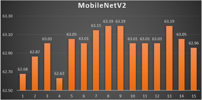
From Table 11, the AdaDelta was the best parameters optimizer in iterations. The batch size with a value of was the best in iterations. The dropout ratio with a value of 28% was the best in iterations. The learning ratio with a value of 0% was the best in iterations. The best achieved distinctive metrics for the loss, accuracy, F1, precision, recall, AUC, and WSM were 0.7374, 64.74%, 64.75%, 64.74%, 64.74%, 0.6687, and 63.19% respectively. The last best achieved combination was in iteration number where its metrics were 0.7360, 64.74%, 64.75%, 64.74%, 64.74%, 0.6692, and 63.19% respectively. All of the WSM scores were above 62%. Fig. 17 shows the WSM curve for the iterations.
Fig. 17.
The WSM Curve for the MobileNetV2.
Xception: Table 12 reports the top-1 combination in each hyperparameters optimization iteration in the optimization iterations for the Xception pre-trained CNN model with the corresponding performance metrics. Each iteration has as the population size where each solution is trained for epochs.
Table 12.
Top-1 combinations for the Xception in the 15 optimization iterations.
| # | Parameters optimizer | Batch size | Dropout ratio | TL learn ratio | Loss | Accuracy | F1 | Precision | Recall | AUC | WSM |
|---|---|---|---|---|---|---|---|---|---|---|---|
| 1 | AdaDelta | 32 | 0.56 | 90% | 0.4595 | 80.81% | 80.80% | 80.81% | 80.81% | 0.8988 | 78.89% |
| 2 | AdaMax | 32 | 0.56 | 100% | 0.1057 | 96.68% | 96.68% | 96.68% | 96.68% | 0.9922 | 94.74% |
| 3 | AdaMax | 32 | 0.56 | 100% | 0.0972 | 97.11% | 97.11% | 97.11% | 97.11% | 0.9939 | 95.20% |
| 4 | AdaMax | 64 | 0.6 | 100% | 0.0955 | 98.08% | 98.08% | 98.08% | 98.08% | 0.9942 | 96.15% |
| 5 | AdaMax | 64 | 0.6 | 100% | 0.0602 | 98.46% | 98.46% | 98.46% | 98.46% | 0.9959 | 96.83% |
| 6 | AdaMax | 64 | 0.6 | 100% | 0.1952 | 96.20% | 96.20% | 96.20% | 96.20% | 0.9842 | 94.05% |
| 7 | AdaMax | 64 | 0.6 | 100% | 0.0969 | 97.40% | 97.40% | 97.40% | 97.40% | 0.9924 | 95.48% |
| 8 | RMSProp | 32 | 0.6 | 100% | 0.1202 | 97.35% | 97.36% | 97.35% | 97.35% | 0.9935 | 95.34% |
| 9 | AdaMax | 64 | 0.6 | 100% | 0.1352 | 96.25% | 96.25% | 96.25% | 96.25% | 0.9882 | 94.21% |
| 10 | AdaMax | 64 | 0.6 | 100% | 0.0897 | 98.03% | 98.03% | 98.03% | 98.03% | 0.9938 | 96.13% |
| 11 | AdaMax | 64 | 0.6 | 100% | 0.1002 | 98.03% | 98.03% | 98.03% | 98.03% | 0.9928 | 96.08% |
| 12 | AdaMax | 64 | 0.6 | 100% | 0.0743 | 97.74% | 97.74% | 97.74% | 97.74% | 0.9956 | 95.97% |
| 13 | AdaMax | 64 | 0.6 | 100% | 0.0701 | 98.46% | 98.46% | 98.46% | 98.46% | 0.9941 | 96.71% |
| 14 | AdaMax | 64 | 0.6 | 100% | 0.0550 | 98.75% | 98.75% | 98.75% | 98.75% | 0.9976 | 97.19% |
| 15 | AdaMax | 64 | 0.6 | 100% | 0.0520 | 98.80% | 98.80% | 98.80% | 98.80% | 0.9972 | 97.29% |
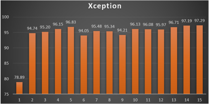
From Table 12, the AdaMax was the best parameters optimizer in iterations. The batch size with a value of was the best in iterations. The dropout ratio with a value of 60% was the best in iterations. The learning ratio with a value of 100% was the best in iterations. The best achieved distinctive metrics for the loss, accuracy, F1, precision, recall, AUC, and WSM were 0.0520, 98.80%, 98.80%, 98.80%, 98.80%, 0.9972, and 97.29% respectively. The best achieved combination was in iteration number where its metrics were 0.0520, 98.80%, 98.80%, 98.80%, 98.80%, 0.9972, and 97.29% respectively. All of the WSM scores were above 78%. Fig. 18 shows the WSM curve for the iterations.
Fig. 18.
The WSM Curve for the Xception.
Table 13 reports the best achieved top-1 combinations in all experiments.
Table 13.
Summary of the best achieved Top-1 combinations in all experiments.
| Experiment | Model | Parameters optimizer | Batch size | Dropout ratio | TL learn ratio | WSM |
|---|---|---|---|---|---|---|
| 1 | VGG16 | SGD | 32 | 0.58 | 80% | 99.02% |
| 2 | VGG19 | SGD | 32 | 0.56 | 80% | 99.31% |
| 3 | ResNet50 | SGD | 32 | 0.6 | 100% | 97.64% |
| 4 | ResNet101 | SGD | 64 | 0.6 | 100% | 96.63% |
| 5 | DenseNet121 | RMSProp | 32 | 0.41 | 75% | 87.96% |
| 6 | DenseNet169 | AdaMax | 32 | 0.36 | 50% | 88.54% |
| 7 | MobileNet | SGD | 64 | 0.6 | 100% | 97.44% |
| 8 | MobileNetV2 | AdaDelta | 32 | 0.28 | 0% | 63.19% |
| 9 | Xception | AdaMax | 64 | 0.6 | 100% | 97.29% |
From Table 13, it is clear that the best pre-trained model was VGG19 as it reported a WSM value of 99.31% while the worst pre-trained model was MobileNetV2 as it reported only 63.19%.
5.3. Comparative study
As noted in Table 13, the 99.31% score was the highest WSM value while 99.33% was the highest achieved accuracy by VGG19. Table 14 constructs a comparative table between the current study and other state-of-the-art studies. They are sorted in descending order. It shows that the current study reported the highest accuracy value among them.
Table 14.
Comparative study with State-of-the-art studies.
| Study | Model | Dataset size | CT or X-ray | Accuracy |
|---|---|---|---|---|
| Khan et al. (2020) | CoroNet | 1,300 | X-ray | 89.60% |
| Hemdan et al. (2020) | COVIDX-Net | 50 | X-ray | 90.00% |
| El Asnaoui and Chawki (2020) | InceptionResNetV2 | 6,087 | X-ray | 92.18% |
| Shah et al. (2021) | VGG19 | 738 | CT | 94.52% |
| Yasar and Ceylan (2021) | MobilenetV2 | 1,396 | CT | 95.99% |
| Toraman et al. (2020) | InstaCovNet-19 | 3,150 | X-ray | 97.24% |
| Apostolopoulos and Mpesiana (2020) | MobileNetV2 | 1,428 | X-ray | 97.40% |
| Ozturk et al. (2020) | DarkCovidNet | 127 | X-ray | 98.08% |
| Nayak, Nayak, Sinha, Arora, and Pachori (2021) | ResNet34 | 500 | X-ray | 98.33% |
| Apostolopoulos and Mpesiana (2020) | VGG19 | 1,428 | X-ray | 98.75% |
| Zhou et al. (2021) | Ensemble Model | 5,000 | CT | 99.05% |
| Current Study | CovH2SD (VGG19) | 15,535 | CT | 99.33% |
6. Conclusions and future work
Unfortunately, the danger of COVID-19 did not end till the moment. Fast diagnosis of patients is the golden key treatment to stop the incredible spread of the virus so that patients can be isolated accordingly. Cost of diagnosis plays another factor, especially for developing countries.
As seen, in this study, a hybrid approach named CovH2SD was suggested to detect the COVID-19 using the Chest Computed Tomography (CT) images. CovH2SD consisted of two internal optimization mechanisms. The first was the parameters’ optimization mechanism which was performed using the deep learning optimizers. They were Adam, NAdam, Ftrl, SGD, AdaMax, AdaGrad, and AdaDelta. The second was the hyperparameters optimization mechanism which was performed using the Harris Hawks Optimization (HHO) algorithm. The used hyperparameters were the parameters optimizer, the dropout ratio, the learning ratio, and the batch size. The HHO algorithm answered the question “Which parameters optimizer with which dropout ratio with which learning ratio with which batch size can report the highest performance measure?” as reported in the experiments.
Transfer learning was targeted using nine pre-trained CNNs. They were ResNet50, ResNet101, VGG16, VGG19, Xception, MobileNetV1, MobileNetV2, DenseNet121, and DenseNet169. Stacking the best models into a single one was applied using FCS and CSS. Nine experiments were applied on the CT images collected from public and shared sources. The used performance metrics were Loss, Accuracy, Precision, Recall, F1-Score, and AUC. The WSM metric is used to solve this multi-objective problem and to compare between the different combinations Six experiments reported a WSM value that was above 96.5%. The top WSM reported value was 99.31% which was higher than the compared studies. This best value was reported by the VGG19 pre-trained CNN model using the SGD parameters’ optimizer, batch size, 56% dropout ratio, and 80% learning ratio.
The proposed approach could reach state-of-the-art performance according to the compared studies. It proved that it is a good candidate in practice. As future work, we aim to expand the suggested approach for multi-class classification problems. We can also upgrade it to apply it to different medical imaging problems. Different optimizers can also be used such as Sparrow Search Algorithm or Manta Ray Foraging Optimization algorithm.
Declaration of Competing Interest
The authors declare that they have no known competing financial interests or personal relationships that could have appeared to influence the work reported in this paper.
Appendix.
Table of abbreviations
Table A.15 presents the “Table of Abbreviations” and is ordered in ascending order.
Table A.15.
Table of abbreviations.
| Abbreviation | Description |
|---|---|
| AdaDelta | Adaptive Delta |
| AdaGrad | Adaptive Gradient |
| Adam | Adaptive Momentum |
| AdaMax | Adaptive Max-Pooling |
| AI | Artificial Intelligence |
| ANN | Artificial Neural Network |
| AUC | Area Under Curve |
| CNN | Convolutional Neural Network |
| COVID-19 | Coronavirus |
| CS | Cuckoo Search |
| CSS | Compact Stacking Stage |
| CT | Computed Tomography |
| DenseNet | Densely Connected Convolutional Networks |
| DL | Deep Learning |
| FC | Fully-Connected |
| FCS | Fast Classification Stage |
| GA | Genetic Algorithms |
| GOA | Grasshopper Optimization Algorithm |
| GWO | Gray Wolf Optimizer |
| HHO | Harris Hawks Optimization |
| LF | Levy Flight |
| NAdam | Nesterov Adaptive Momentum |
| PSO | Particle Swarm Optimization |
| QS | Quality Space |
| ReLU | Rectified Linear Unit |
| ResNet | Residual Network |
| RMSProp | Root Mean Square Propagation |
| RT-PCR | Reverse Transcription Polymerase Chain Reaction |
| SGD | Stochastic Gradient Descent |
| TL | Transfer Learning |
| WHO | World Health Organization |
| WSM | Weighted Sum Method |
References
- Abdulazeem Y., Balaha H.M., Bahgat W.M., Badawy M. Human action recognition based on transfer learning approach. IEEE Access. 2021 [Google Scholar]
- Abiodun O.I., Jantan A., Omolara A.E., Dada K.V., Mohamed N.A., Arshad H. State-of-the-art in artificial neural network applications: A survey. Heliyon. 2018;4(11) doi: 10.1016/j.heliyon.2018.e00938. [DOI] [PMC free article] [PubMed] [Google Scholar]
- Albawi S., Mohammed T.A., Al-Zawi S. 2017 international conference on engineering and technology. IEEE; 2017. Understanding of a convolutional neural network; pp. 1–6. [Google Scholar]
- Apostolopoulos I.D., Mpesiana T.A. Covid-19: automatic detection from X-ray images utilizing transfer learning with convolutional neural networks. Physical and Engineering Sciences in Medicine. 2020:1. doi: 10.1007/s13246-020-00865-4. [DOI] [PMC free article] [PubMed] [Google Scholar]
- Ardakani A.A., Kanafi A.R., Acharya U.R., Khadem N., Mohammadi A. Application of deep learning technique to manage COVID-19 in routine clinical practice using CT images: Results of 10 convolutional neural networks. Computers in Biology and Medicine. 2020 doi: 10.1016/j.compbiomed.2020.103795. [DOI] [PMC free article] [PubMed] [Google Scholar]
- Aslan M.F., Unlersen M.F., Sabanci K., Durdu A. CNN-based transfer learning–BiLSTM network: A novel approach for COVID-19 infection detection. Applied Soft Computing. 2020;98 doi: 10.1016/j.asoc.2020.106912. [DOI] [PMC free article] [PubMed] [Google Scholar]
- Bahgat W.M., Balaha H.M., AbdulAzeem Y., Badawy M.M. An optimized transfer learning-based approach for automatic diagnosis of COVID-19 from chest X-ray images. PeerJ Computer Science. 2021;7 doi: 10.7717/peerj-cs.555. [DOI] [PMC free article] [PubMed] [Google Scholar]
- Balaha H.M., Ali H.A., Badawy M. Automatic recognition of handwritten Arabic characters: a comprehensive review. Neural Computing and Applications. 2021;33(7):3011–3034. [Google Scholar]
- Balaha H.M., Ali H.A., Saraya M., Badawy M. A new Arabic handwritten character recognition deep learning system (AHCR-DLS) Neural Computing and Applications. 2021;33(11):6325–6367. [Google Scholar]
- Balaha H.M., Ali H.A., Youssef E.K., Elsayed A.E., Samak R.A., Abdelhaleem M.S., et al. Recognizing arabic handwritten characters using deep learning and genetic algorithms. Multimedia Tools and Applications. 2021:1–37. [Google Scholar]
- Balaha H.M., Saafan M.M. Automatic Exam Correction Framework (AECF) for the MCQs, essays, and equations matching. IEEE Access. 2021;9:32368–32389. [Google Scholar]
- Bao X., Jia H., Lang C. A novel hybrid Harris hawks optimization for color image multilevel thresholding segmentation. IEEE Access. 2019;7:76529–76546. [Google Scholar]
- Başaran E., Cömert Z., Çelik Y. Convolutional neural network approach for automatic tympanic membrane detection and classification. Biomedical Signal Processing and Control. 2020;56 [Google Scholar]
- Bottou L. Neural networks: Tricks of the trade. Springer; 2012. Stochastic gradient descent tricks; pp. 421–436. [Google Scholar]
- Celik Y., Talo M., Yildirim O., Karabatak M., Acharya U.R. Automated invasive ductal carcinoma detection based using deep transfer learning with whole-slide images. Pattern Recognition Letters. 2020;133:232–239. [Google Scholar]
- Chen H., Jiao S., Wang M., Heidari A.A., Zhao X. Parameters identification of photovoltaic cells and modules using diversification-enriched Harris hawks optimization with chaotic drifts. Journal of Cleaner Production. 2020;244 URL http://www.sciencedirect.com/science/article/pii/S0959652619336480. [Google Scholar]
- Chollet, F. (2017). Xception: Deep learning with depthwise separable convolutions. In Proceedings of the IEEE conference on computer vision and pattern recognition (pp. 1251–1258).
- Cui Z., Xue F., Cai X., Cao Y., Wang G.-g., Chen J. Detection of malicious code variants based on deep learning. IEEE Transactions on Industrial Informatics. 2018;14(7):3187–3196. [Google Scholar]
- Deepak S., Ameer P. Brain tumor classification using deep CNN features via transfer learning. Computers in Biology and Medicine. 2019;111 doi: 10.1016/j.compbiomed.2019.103345. [DOI] [PubMed] [Google Scholar]
- Dogo E., Afolabi O., Nwulu N., Twala B., Aigbavboa C. 2018 international conference on computational techniques, electronics and mechanical systems. IEEE; 2018. A comparative analysis of gradient descent-based optimization algorithms on convolutional neural networks; pp. 92–99. [Google Scholar]
- Dorj U.-O., Lee K.-K., Choi J.-Y., Lee M. The skin cancer classification using deep convolutional neural network. Multimedia Tools and Applications. 2018;77(8):9909–9924. [Google Scholar]
- Dozat T. 2016. Incorporating nesterov momentum into adam. [Google Scholar]
- El Asnaoui K., Chawki Y. Using X-ray images and deep learning for automated detection of coronavirus disease. Journal of Biomolecular Structure and Dynamics. 2020:1–12. doi: 10.1080/07391102.2020.1767212. [DOI] [PMC free article] [PubMed] [Google Scholar]
- El-Gendy E.M., Saafan M.M., Elksas M.S., Saraya S.F., Areed F.F. Applying hybrid genetic–PSO technique for tuning an adaptive PID controller used in a chemical process. Soft Computing. 2020;24(5):3455–3474. [Google Scholar]
- Feng Y., Wang G.-G., Dong J., Wang L. Opposition-based learning monarch butterfly optimization with Gaussian perturbation for large-scale 0-1 knapsack problem. Computers and Electrical Engineering. 2018;67:454–468. [Google Scholar]
- Gao F., Wu T., Li J., Zheng B., Ruan L., Shang D., et al. SD-CNN: A shallow-deep CNN for improved breast cancer diagnosis. Computerized Medical Imaging and Graphics. 2018;70:53–62. doi: 10.1016/j.compmedimag.2018.09.004. [DOI] [PubMed] [Google Scholar]
- Golilarz N.A., Gao H., Demirel H. Satellite image de-noising with Harris hawks meta heuristic optimization algorithm and improved adaptive generalized gaussian distribution threshold function. IEEE Access. 2019;7:57459–57468. [Google Scholar]
- Gour M., Jain S. 2020. Stacked convolutional neural network for diagnosis of covid-19 disease from X-ray images. arXiv preprint arXiv:2006.13817. [Google Scholar]
- Guo, Y., Shi, H., Kumar, A., Grauman, K., Rosing, T., & Feris, R. (2019). Spottune: transfer learning through adaptive fine-tuning. In Proceedings of the IEEE/CVF conference on computer vision and pattern recognition (pp. 4805–4814).
- Gupta A., Anjum S., Gupta S., Katarya R. InstaCovNet-19: A deep learning classification model for the detection of COVID-19 patients using chest X-ray. Applied Soft Computing. 2021;99 doi: 10.1016/j.asoc.2020.106859. URL http://www.sciencedirect.com/science/article/pii/S1568494620307973. [DOI] [PMC free article] [PubMed] [Google Scholar]
- He, K., Zhang, X., Ren, S., & Sun, J. (2016). Deep residual learning for image recognition. In Proceedings of the IEEE conference on computer vision and pattern recognition (pp. 770–778).
- Heidari A.A., Mirjalili S., Faris H., Aljarah I., Mafarja M., Chen H. Harris hawks optimization: Algorithm and applications. Future Generation Computer Systems. 2019;97:849–872. [Google Scholar]
- Hemdan E.E.-D., Shouman M.A., Karar M.E. 2020. Covidx-net: A framework of deep learning classifiers to diagnose covid-19 in X-ray images. arXiv preprint arXiv:2003.11055. [Google Scholar]
- Holland J.H. Genetic algorithms. Scientific American. 1992;267(1):66–73. [Google Scholar]
- Howard A.G., Zhu M., Chen B., Kalenichenko D., Wang W., Weyand T., et al. 2017. Mobilenets: Efficient convolutional neural networks for mobile vision applications. arXiv preprint arXiv:1704.04861. [Google Scholar]
- Huang, G., Liu, Z., Van Der Maaten, L., & Weinberger, K. Q. (2017). Densely connected convolutional networks. In Proceedings of the IEEE conference on computer vision and pattern recognition (pp. 4700–4708).
- Huynh B.Q., Li H., Giger M.L. Digital mammographic tumor classification using transfer learning from deep convolutional neural networks. Journal of Medical Imaging. 2016;3(3) doi: 10.1117/1.JMI.3.3.034501. [DOI] [PMC free article] [PubMed] [Google Scholar]
- Jia H., Lang C., Oliva D., Song W., Peng X. Dynamic Harris hawks optimization with mutation mechanism for satellite image segmentation. Remote Sensing. 2019;11(12):1421. [Google Scholar]
- Ju C., Bibaut A., van der Laan M. The relative performance of ensemble methods with deep convolutional neural networks for image classification. Journal of Applied Statistics. 2018;45(15):2800–2818. doi: 10.1080/02664763.2018.1441383. [DOI] [PMC free article] [PubMed] [Google Scholar]
- Kasinathan G., Jayakumar S., Gandomi A.H., Ramachandran M., Fong S.J., Patan R. Automated 3-D lung tumor detection and classification by an active contour model and CNN classifier. Expert Systems with Applications. 2019;134:112–119. [Google Scholar]
- Kennedy J., Eberhart R. Proceedings of ICNN’95-international conference on neural networks, Vol. 4. IEEE; 1995. Particle swarm optimization; pp. 1942–1948. [Google Scholar]
- Khan A.I., Shah J.L., Bhat M.M. Coronet: A deep neural network for detection and diagnosis of COVID-19 from chest X-ray images. Computer Methods and Programs in Biomedicine. 2020 doi: 10.1016/j.cmpb.2020.105581. [DOI] [PMC free article] [PubMed] [Google Scholar]
- Kingma D.P., Ba J. 2014. Adam: A method for stochastic optimization. arXiv preprint arXiv:1412.6980. [Google Scholar]
- Krizhevsky A., Sutskever I., Hinton G.E. Imagenet classification with deep convolutional neural networks. Advances in Neural Information Processing Systems. 2012;25:1097–1105. [Google Scholar]
- Li J., Li Y.-x., Tian S.-s., Xia J.-l. An improved cuckoo search algorithm with self-adaptive knowledge learning. Neural Computing and Applications. 2019:1–31. [Google Scholar]
- Li J., Li Y.-x., Tian S.-s., Zou J. Dynamic cuckoo search algorithm based on Taguchi opposition-based search. International Journal of Bio-Inspired Computation. 2019;13(1):59–69. [Google Scholar]
- Li W., Wang G.-G. Elephant herding optimization using dynamic topology and biogeography-based optimization based on learning for numerical optimization. Engineering with Computers. 2021:1–29. [Google Scholar]
- Li W., Wang G.-G., Alavi A.H. Learning-based elephant herding optimization algorithm for solving numerical optimization problems. Knowledge-Based Systems. 2020;195 [Google Scholar]
- Li G., Wang G.-G., Dong J., Yeh W.-C., Li K. DLEA: A dynamic learning evolution algorithm for many-objective optimization. Information Sciences. 2021;574:567–589. [Google Scholar]
- Li W., Wang G.-G., Gandomi A.H. A survey of learning-based intelligent optimization algorithms. Archives of Computational Methods in Engineering. 2021:1–19. [Google Scholar]
- Li G., Wang G.-G., Wang S. Two-population coevolutionary algorithm with dynamic learning strategy for many-objective optimization. Mathematics. 2021;9(4):420. [Google Scholar]
- Li J., Xiao D.-d., Lei H., Zhang T., Tian T. Using cuckoo search algorithm with q-learning and genetic operation to solve the problem of logistics distribution center location. Mathematics. 2020;8(2):149. [Google Scholar]
- Li Y., Yao L., Li J., Chen L., Song Y., Cai Z., et al. Stability issues of RT-PCR testing of SARS-CoV-2 for hospitalized patients clinically diagnosed with COVID-19. Journal of Medical Virology. 2020 doi: 10.1002/jmv.25786. [DOI] [PMC free article] [PubMed] [Google Scholar]
- Livingstone D.J. Springer; 2008. Artificial neural networks: Methods and applications. [PubMed] [Google Scholar]
- Luo L., Xiong Y., Liu Y., Sun X. 2019. Adaptive gradient methods with dynamic bound of learning rate. arXiv preprint arXiv:1902.09843. [Google Scholar]
- Mangal A., Kalia S., Rajgopal H., Rangarajan K., Namboodiri V., Banerjee S., et al. 2020. CovidAID: COVID-19 detection using chest X-ray. arXiv preprint arXiv:2004.09803. [Google Scholar]
- Marques G., Agarwal D., de la Torre Díez I. Automated medical diagnosis of COVID-19 through EfficientNet convolutional neural network. Applied Soft Computing. 2020;96 doi: 10.1016/j.asoc.2020.106691. [DOI] [PMC free article] [PubMed] [Google Scholar]
- Mirjalili S., Mirjalili S.M., Lewis A. Grey wolf optimizer. Advances in Engineering Software. 2014;69:46–61. [Google Scholar]
- Najafabadi M.M., Villanustre F., Khoshgoftaar T.M., Seliya N., Wald R., Muharemagic E. Deep learning applications and challenges in big data analytics. Journal of Big Data. 2015;2(1):1. [Google Scholar]
- Nan X., Bao L., Zhao X., Zhao X., Sangaiah A.K., Wang G.-G., et al. Epul: an enhanced positive-unlabeled learning algorithm for the prediction of pupylation sites. Molecules. 2017;22(9):1463. doi: 10.3390/molecules22091463. [DOI] [PMC free article] [PubMed] [Google Scholar]
- Nayak S.R., Nayak D.R., Sinha U., Arora V., Pachori R.B. Application of deep learning techniques for detection of COVID-19 cases using chest X-ray images: A comprehensive study. Biomedical Signal Processing and Control. 2021;64 doi: 10.1016/j.bspc.2020.102365. [DOI] [PMC free article] [PubMed] [Google Scholar]
- Ning W., Lei S., Yang J., Cao Y., Jiang P., Yang Q., et al. 2020. iCTCF: an integrative resource of chest computed tomography images and clinical features of patients with COVID-19 pneumonia. [Google Scholar]
- Nour M., Cömert Z., Polat K. A novel medical diagnosis model for COVID-19 infection detection based on deep features and Bayesian optimization. Applied Soft Computing. 2020;97 doi: 10.1016/j.asoc.2020.106580. [DOI] [PMC free article] [PubMed] [Google Scholar]
- Orenstein E.C., Beijbom O. 2017 IEEE winter conference on applications of computer vision. IEEE; 2017. Transfer learning and deep feature extraction for planktonic image data sets; pp. 1082–1088. [Google Scholar]
- Ozturk T., Talo M., Yildirim E.A., Baloglu U.B., Yildirim O., Acharya U.R. Automated detection of COVID-19 cases using deep neural networks with X-ray images. Computers in Biology and Medicine. 2020 doi: 10.1016/j.compbiomed.2020.103792. [DOI] [PMC free article] [PubMed] [Google Scholar]
- Pan S.J., Yang Q. A survey on transfer learning. IEEE Transactions on Knowledge and Data Engineering. 2009;22(10):1345–1359. [Google Scholar]
- Qin Z., Yu F., Liu C., Chen X. 2018. How convolutional neural network see the world-A survey of convolutional neural network visualization methods. arXiv preprint arXiv:1804.11191. [Google Scholar]
- Rahimzadeh M., Attar A., Sakhaei S.M. 2020. A fully automated deep learning-based network for detecting covid-19 from a new and large lung CT scan dataset. MedRxiv. [DOI] [PMC free article] [PubMed] [Google Scholar]
- Rubin G.D., Ryerson C.J., Haramati L.B., Sverzellati N., Kanne J.P., Raoof S., et al. The role of chest imaging in patient management during the COVID-19 pandemic: a multinational consensus statement from the fleischner society. Chest. 2020 doi: 10.1016/j.chest.2020.04.003. [DOI] [PMC free article] [PubMed] [Google Scholar]
- Ruder S. 2016. An overview of gradient descent optimization algorithms. arXiv preprint arXiv:1609.04747. [Google Scholar]
- Saafan M.M., El-Gendy E.M. IWOSSA: An improved whale optimization salp swarm algorithm for solving optimization problems. Expert Systems with Applications. 2021;176 doi: 10.1016/j.eswa.2021.115805. [DOI] [PMC free article] [PubMed] [Google Scholar]
- Salamon J., Bello J.P. Deep convolutional neural networks and data augmentation for environmental sound classification. IEEE Signal Processing Letters. 2017;24(3):279–283. [Google Scholar]
- Sandler, M., Howard, A., Zhu, M., Zhmoginov, A., & Chen, L.-C. (2018). Mobilenetv2: Inverted residuals and linear bottlenecks. In Proceedings of the IEEE conference on computer vision and pattern recognition (pp. 4510–4520).
- Saremi S., Mirjalili S., Lewis A. Grasshopper optimisation algorithm: theory and application. Advances in Engineering Software. 2017;105:30–47. [Google Scholar]
- Shah V., Keniya R., Shridharani A., Punjabi M., Shah J., Mehendale N. Diagnosis of COVID-19 using CT scan images and deep learning techniques. Emergency Radiology. 2021:1–9. doi: 10.1007/s10140-020-01886-y. [DOI] [PMC free article] [PubMed] [Google Scholar]
- Shorten C., Khoshgoftaar T.M. A survey on image data augmentation for deep learning. Journal of Big Data. 2019;6(1):60. doi: 10.1186/s40537-021-00492-0. [DOI] [PMC free article] [PubMed] [Google Scholar]
- Simonyan K., Zisserman A. 2014. Very deep convolutional networks for large-scale image recognition. arXiv preprint arXiv:1409.1556. [Google Scholar]
- Toraman S., Alakus T.B., Turkoglu I. Convolutional capsnet: A novel artificial neural network approach to detect COVID-19 disease from X-ray images using capsule networks. Chaos, Solitons & Fractals. 2020;140 doi: 10.1016/j.chaos.2020.110122. URL http://www.sciencedirect.com/science/article/pii/S0960077920305191. [DOI] [PMC free article] [PubMed] [Google Scholar]
- Vani S., Rao T.M. 2019 3rd international conference on trends in electronics and informatics. IEEE; 2019. An experimental approach towards the performance assessment of various optimizers on convolutional neural network; pp. 331–336. [Google Scholar]
- Wang S.-C. Interdisciplinary computing in Java programming. Springer; 2003. Artificial neural network; pp. 81–100. [Google Scholar]
- Wang G.-G., Deb S., Gandomi A.H., Alavi A.H. Opposition-based krill herd algorithm with Cauchy mutation and position clamping. Neurocomputing. 2016;177:147–157. [Google Scholar]
- Wang G., Guo L., Duan H. Wavelet neural network using multiple wavelet functions in target threat assessment. The Scientific World Journal. 2013;2013 doi: 10.1155/2013/632437. [DOI] [PMC free article] [PubMed] [Google Scholar]
- Wang Y., Kang H., Liu X., Tong Z. Combination of RT-qPCR testing and clinical features for diagnosis of COVID-19 facilitates management of SARS-CoV-2 outbreak. Journal of Medical Virology. 2020;92(6):538–539. doi: 10.1002/jmv.25721. [DOI] [PMC free article] [PubMed] [Google Scholar]
- Wang G.-G., Lu M., Dong Y.-Q., Zhao X.-J. Self-adaptive extreme learning machine. Neural Computing and Applications. 2016;27(2):291–303. [Google Scholar]
- Weiss K., Khoshgoftaar T.M., Wang D. A survey of transfer learning. Journal of Big Data. 2016;3(1):1–40. [Google Scholar]
- Wolpert D.H. Stacked generalization. Neural Networks. 1992;5(2):241–259. [Google Scholar]
- Wong H.Y.F., Lam H.Y.S., Fong A.H.-T., Leung S.T., Chin T.W.-Y., Lo C.S.Y., et al. Frequency and distribution of chest radiographic findings in COVID-19 positive patients. Radiology. 2020 doi: 10.1148/radiol.2020201160. [DOI] [PMC free article] [PubMed] [Google Scholar]
- Wu L., Shen C., Hengel A.v.d. 2016. Personnet: Person re-identification with deep convolutional neural networks. arXiv preprint arXiv:1601.07255. [Google Scholar]
- Xu S., Li Y. Beware of the second wave of COVID-19. The Lancet. 2020;395(10233):1321–1322. doi: 10.1016/S0140-6736(20)30845-X. [DOI] [PMC free article] [PubMed] [Google Scholar]
- Xu L., Ren J.S., Liu C., Jia J. Advances in neural information processing systems. 2014. Deep convolutional neural network for image deconvolution; pp. 1790–1798. [Google Scholar]
- Yamashita R., Nishio M., Do R.K.G., Togashi K. Convolutional neural networks: an overview and application in radiology. Insights Into Imaging. 2018;9(4):611–629. doi: 10.1007/s13244-018-0639-9. [DOI] [PMC free article] [PubMed] [Google Scholar]
- Yang X.-S., Deb S. Engineering optimisation by cuckoo search. International Journal of Mathematical Modelling and Numerical Optimisation. 2010;1(4):330–343. [Google Scholar]
- Yasar H., Ceylan M. A novel comparative study for detection of Covid-19 on CT lung images using texture analysis, machine learning, and deep learning methods. Multimedia Tools and Applications. 2021;80(4):5423–5447. doi: 10.1007/s11042-020-09894-3. [DOI] [PMC free article] [PubMed] [Google Scholar]
- Yi J.-H., Wang J., Wang G.-G. Improved probabilistic neural networks with self-adaptive strategies for transformer fault diagnosis problem. Advances in Mechanical Engineering. 2016;8(1) [Google Scholar]
- Yousri D., Abd Elaziz M., Abualigah L., Oliva D., Al-qaness M.A., Ewees A.A. COVID-19 X-ray images classification based on enhanced fractional-order cuckoo search optimizer using heavy-tailed distributions. Applied Soft Computing. 2021;101 doi: 10.1016/j.asoc.2020.107052. URL http://www.sciencedirect.com/science/article/pii/S156849462030990X. [DOI] [PMC free article] [PubMed] [Google Scholar]
- Zaim S., Chong J.H., Sankaranarayanan V., Harky A. COVID-19 and multiorgan response. Current Problems in Cardiology. 2020;45(8) doi: 10.1016/j.cpcardiol.2020.100618. URL http://www.sciencedirect.com/science/article/pii/S0146280620300955. [DOI] [PMC free article] [PubMed] [Google Scholar]
- Zeiler M.D. 2012. Adadelta: an adaptive learning rate method. arXiv preprint arXiv:1212.5701. [Google Scholar]
- Zhang K., Liu X., Shen J., Li Z., Sang Y., Wu X., et al. Clinically applicable AI system for accurate diagnosis, quantitative measurements, and prognosis of covid-19 pneumonia using computed tomography. Cell. 2020 doi: 10.1016/j.cell.2020.08.029. [DOI] [PMC free article] [PubMed] [Google Scholar]
- Zhang Y., Lobo-Mueller E.M., Karanicolas P., Gallinger S., Haider M.A., Khalvati F. CNN-based survival model for pancreatic ductal adenocarcinoma in medical imaging. BMC Medical Imaging. 2020;20(1):1–8. doi: 10.1186/s12880-020-0418-1. [DOI] [PMC free article] [PubMed] [Google Scholar]
- Zhang C., Pan X., Li H., Gardiner A., Sargent I., Hare J., et al. A hybrid MLP-CNN classifier for very fine resolution remotely sensed image classification. ISPRS Journal of Photogrammetry and Remote Sensing. 2018;140:133–144. [Google Scholar]
- Zhang Y.-D., Zhang Z., Zhang X., Wang S.-H. MIDCAN: A multiple input deep convolutional attention network for Covid-19 diagnosis based on chest CT and chest X-ray. Pattern Recognition Letters. 2021 doi: 10.1016/j.patrec.2021.06.021. [DOI] [PMC free article] [PubMed] [Google Scholar]
- Zhang Y., Zhang X., Zhu W. ANC: attention network for COVID-19 explainable diagnosis based on convolutional block attention module. CMES-Computer Modeling in Engineering and Sciences. 2021;127(3) [Google Scholar]
- Zhao J., Zhang Y., He X., Xie P. 2020. Covid-ct-dataset: a CT scan dataset about covid-19. arXiv preprint arXiv:2003.13865. [Google Scholar]
- Zhou T., Lu H., Yang Z., Qiu S., Huo B., Dong Y. The ensemble deep learning model for novel COVID-19 on CT images. Applied Soft Computing. 2021;98 doi: 10.1016/j.asoc.2020.106885. [DOI] [PMC free article] [PubMed] [Google Scholar]
- Zhuang F., Qi Z., Duan K., Xi D., Zhu Y., Zhu H., et al. A comprehensive survey on transfer learning. Proceedings of the IEEE. 2020;109(1):43–76. [Google Scholar]


