Likelihood-based deconvolution of bulk gene expression data using single-cell references

Abstract

Direct comparison of bulk gene expression profiles is complicated by distinct cell type mixtures in each sample that obscure whether observed differences are actually caused by changes in the expression levels themselves or are simply a result of differing cell type compositions. Single-cell technology has made it possible to measure gene expression in individual cells, achieving higher resolution at the expense of increased noise. If carefully incorporated, such single-cell data can be used to deconvolve bulk samples to yield accurate estimates of the true cell type proportions, thus enabling one to disentangle the effects of differential expression and cell type mixtures. Here, we propose a generative model and a likelihood-based inference method that uses asymptotic statistical theory and a novel optimization procedure to perform deconvolution of bulk RNA-seq data to produce accurate cell type proportion estimates. We show the effectiveness of our method, called RNA-Sieve, across a diverse array of scenarios involving real data and discuss extensions made uniquely possible by our probabilistic framework, including a demonstration of well-calibrated confidence intervals.

Bulk RNA sequencing (RNA-seq) has proven a useful tool to investigate transcriptomic variation across organs, individuals, and various other biological conditions (Melé et al. 2015; Sudmant et al. 2015). Despite many successes, this technology's full potential is inherently limited because each experiment measures the average gene expression among a large group of cells, the composition of which is unknown. Thus, despite the reduction in technical and biological variability attained by averaging, bulk experiments may be confounded by cell type proportions when considering heterogeneous cell mixtures (Lowe and Rakyan 2014; Shiwa et al. 2016). Such confounding impedes the direct comparison of samples, possibly leading to the spurious or missed inference of biologically relevant genes when attempting to identify clinically important differences. Moreover, cell type compositions are often independently informative of biological processes including organ function (Cabrera et al. 2006; Kalisky et al. 2013; Yu and He 2017; Hagenauer et al. 2018) and development (Hu et al. 2017; Hagenauer et al. 2018). For example, cell type infiltration has been found to correlate with disease progression, disease status, and complex phenomena such as aging (Funada et al. 2003; Bremnes et al. 2016; Bense et al. 2017; Stout et al. 2017; Zhou et al. 2019). Unlike bulk experiments, single-cell technologies allow us to query the transcriptome at the resolution of individual cells. Resulting analyses often seek to characterize the heterogeneity within, or the differences between, specified cell types (Saliba et al. 2014). By isolating the expression patterns of measured cell types, single-cell gene expression data can provide a reference to aid the inference of the cell type compositions of bulk samples; this process is known as deconvolution.

Computational rather than experimental estimation of cell type compositions is attractive for several reasons. Single-cell experiments are more expensive than their bulk counterparts and require heightened technical expertise to perform, often rendering the large-scale generation of single-cell gene expression data infeasible (Goldman et al. 2019). Furthermore, even when performed correctly, many protocols fail to capture cell types in an unbiased fashion, meaning empirical cell type proportions often are not reliable estimators of true organ/tissue compositions (Trapnell 2015). Finally, deconvolution can be applied to the deep compendium of available bulk RNA-seq data to refine earlier analyses and probe previously unanswerable or heretofore unformulated questions. Consequently, the computational deconvolution problem has become a topic of intense methodological research, as detailed in Avila Cobos et al. (2018). The problem may be represented mathematically as

$$M\mathit{\alpha }=\mathit{b},$$ (1)

where M is a gene-by-cell type matrix of cell type–specific gene expression averages, α is a vector of cell type mixing proportions, and b is a vector of gene expression values in a bulk RNA-seq experiment. Depending on which of M, α, and b are measured, different approaches are appropriate. We focus on the case in which both M and b have been observed, albeit noisily, and it remains to infer α; this is known as supervised deconvolution. Early approaches frequently used predefined marker genes for well-studied cell types, restricting their applicability. More recent methods formulate the problem as a regression task to be solved by variants of non-negative least squares, for example, MuSiC (Wang et al. 2019), DWLS (Tsoucas et al. 2019), SCDC (Dong et al. 2021), and Bisque (Jew et al. 2020), or with more sophisticated machine learning techniques, such as CIBERSORTx (Newman et al. 2019) and Scaden (Menden et al. 2020). Although each paradigm presents its own strengths, both fail to replicate the benefits of explicit generative modeling. The resulting algorithms may perform well, but often lack the flexibility to extend beyond the estimation of cell type proportions.

We hence propose RNA-Sieve, a method that uses asymptotic theory and a novel optimization procedure to solve a probabilistic model of deconvolution via maximum likelihood estimation. We show its highly capable performance across a diverse array of scenarios, including different organs, cell types, and practical challenges. We then highlight newly opened avenues for continued development made feasible by our generative framework, including confidence regions.

Results

Method overview

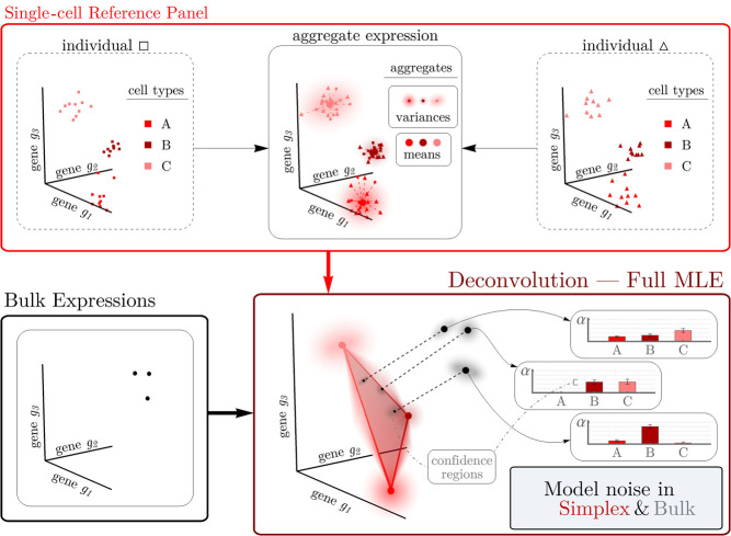
Although a single run of bulk RNA-seq produces a solitary gene expression vector, myriad cells contribute to this measurement. The obtained profile is thus a composite snapshot of the gene expression levels of numerous individual, putatively independent cells. Under an assumption that cells of the same type behave similarly, this large number of cells permits the application of the central limit theorem (CLT) and its contingent wealth of asymptotic normal approximations. This renders the marginal gene expression distribution for an arbitrary cell in the bulk sample as a straightforward mixture distribution (see Equation 2 in Methods). The resulting CLT-derived likelihood only depends on the cell type proportions in the bulk sample and each cell type's gene expression means and variances. To estimate the requisite cell type–specific moments, RNA-Sieve uses gene expression measurements from scRNA-seq experiments. We further model the estimation error of these computed quantities by again invoking the CLT, building a full composite likelihood using normal distributions. To infer cell type proportions, we implement a customized maximum likelihood estimation procedure designed to ensure accurate and robust results. Our alternating optimization scheme is split into two components to better avoid suboptimal local minima, and a final projection step avoids slow convergence. We also incorporate a gene filtering procedure explicitly devised to improve cross-protocol stability, a crucial concern given that single-cell and bulk experiments are performed using different technologies. Our algorithm also performs joint deconvolutions, leveraging multiple samples to produce more reliable estimates while parallelizing much of the optimization. In this setting, each bulk sample denoises the single-cell reference regardless of its mixture proportions, leading to improved statistical performance. Finally, our likelihood-based model allows us to pursue extensions that are infeasible using prior approaches. A notable example includes confidence regions for estimates (see “Extension to confidence regions”), among others (Discussion). We present full mathematical and computational details in Methods, and Figure 1 displays a schematic.

Figure 1.

The RNA-Sieve pipeline. After applying a filtering procedure to scRNA-seq data, RNA-Sieve builds reference matrices for the mean and variance of expression for each gene across cell types. Using these estimates and bulk RNA-seq data, it performs joint deconvolution via maximum likelihood estimation by expressly modeling noise both in the reference and bulk data, yielding cell type proportion estimates and confidence regions for each sample.

Performance in pseudobulk experiments

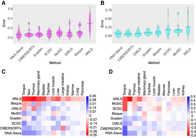
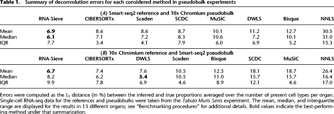
To establish RNA-Sieve's effectiveness, we performed in silico experiments in which we built “pseudobulks” by aggregating reads from labeled cells in known proportions. Our scRNA-seq data come from the Tabula Muris Senis Consortium (The Tabula Muris Consortium 2020), and we considered 13 organs with between two and 11 cell types per organ. Moreover, as counts were generated via both the Smart-seq2 and 10x Chromium protocols for each organ, convenient cross-protocol comparisons are possible. These are particularly important given that the generation of bulk and single-cell RNA-seq samples requires different techniques. To evaluate RNA-Sieve, we compared its performance to that of six recently published methods as well as non-negative least squares (NNLS). Performance was assessed for each organ by computing the L₁ distance (absolute difference) between inferred and true proportions and dividing by the number of cell types present. Further details are provided in “Benchmarking procedures.” We found that RNA-Sieve produced the smallest mean error in both possible reference/bulk configurations (Fig. 2A,B; Table 1; for full results, see Supplemental Table S1). To better understand performance, we also visualized errors when aggregating by organ (i.e., the column-wise distributions of the checkerboard plots in Fig. 2C,D; see Supplemental Fig. S1). Our strong performance across organs regardless of the number of cell types or similarities among them suggests that RNA-Sieve is versatile over a range of scenarios. Finally, we directly compared each method's errors to those of RNA-Sieve on the same deconvolution tasks (given by the row-wise distributions of the checkerboards in Fig. 2C,D; see Supplemental Fig. S2). In each case, RNA-Sieve produced smaller errors than the other methods a majority of the time.

Figure 2.

Distribution of errors for each method in pseudobulk experiments. Pseudobulk experiments were performed in 13 different organs using data from the Tabula Muris Senis experiment. Errors were computed as the average L₁ error across cell types in each organ. (A,C) Smart-seq2 reference, 10x Chromium pseudobulk. (B,D) 10x Chromium pseudobulk, Smart-seq2 pseudobulk. In the violin plots (A,B), horizontal black bars correspond to the mean error and methods are ordered left to right from lowest to greatest mean error. In the grid plots (C,D), methods and organs were ordered using SVD-induced clustering. Roughly speaking, the methods from top to bottom are characterized by improving performance, whereas the organs from left to right are characterized by decreasing variability in different methods’ performances. Color indicates the difference between the average error across methods in that organ; deeper shades of red (blue) indicate poor (good) relative performance. See Supplemental Table S2 for context regarding the cell types present in each organ.

Table 1.

Summary of deconvolution errors for each considered method in pseudobulk experiments

Although RNA-Sieve's nominal improvement in the average per-cell-type L₁ metric may initially appear minor, a typical tissue consists of several cell types; thus the overall error may accumulate rapidly. The constraint that mixture proportions sum to 1 means such reductions in error are likely to be meaningful; inferential errors of the same order as common cell type proportions make it easy to arrive at incorrect biological conclusions, especially in more complex tissues with many cell types. Supplemental Figure S3 shows a representative example of seemingly minor average per-cell-type improvement resulting in comparatively major individual-cell-type differences. Other error metrics are more sensitive to different aspects of performance and may detect such improvements more reliably, and these are explored below (“Benchmarking procedures”). Because one must consider multiple distinct algorithms, tissues, cell types, and experimental protocols, any benchmarking evaluation must necessarily consist of a large number of combinations. Between these many factors and the random nature of the data, it is (even theoretically) nearly impossible for any one algorithm to dominate the others in all situations (as is recognized and discussed in Menden et al. 2020). We believe that evaluation should therefore focus on aggregate measures of accuracy across many situations. We hence supplement Table 1 and Figure 2 with Table 2, which presents the mean ranks of all eight algorithms aggregated across all (26) cross-protocol experiments using the L₁, L₂, L_∞, and KL error quantifications to assess different aspects of performance (see “Benchmarking procedures”). We find RNA-Sieve outperforms its nearest competitor by roughly one-half rank regardless of error metric, a gap that is at least as large as those between other neighboring methods (NNLS excluded). Having shown RNA-Sieve's ability to produce accurate results in the intended use case, we explored its performance under various settings of model misspecification in which the cell types in the reference fail to match those in the bulk samples. Our experiments confirm that, to the extent possible, RNA-Sieve produces robust and interpretable inferences even in these settings (Supplemental Text S1.1; Supplemental Figs. S4–S7).

Table 2.

Mean ranking of algorithms under various error metrics

Validation with real bulk RNA-seq data

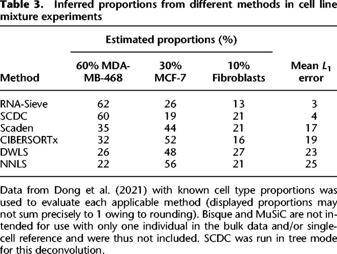
In rare instances, bulk RNA-seq samples with known or experimentally estimated cell type proportions are available. We considered three such data sets to evaluate RNA-Sieve under realistic conditions. The first is a bulk RNA-seq mixture of two human breast cancer cell lines and fibroblasts (60% MDA-MB-468, 30% MCF-7, 10% fibroblasts) with accompanying scRNA-seq data published in Dong et al. (2021). As shown in Table 3, RNA-Sieve yields highly accurate results, attaining the lowest average error among all methods. With the exception of SCDC, other methods overestimated the bulk fraction of the MCF-7 cell line while significantly underestimating the MDA-MB-468 cell line, and most methods substantially overestimated the fibroblast proportion.

Table 3.

Inferred proportions from different methods in cell line mixture experiments

Because this single experiment contains three cell types and one bulk sample, we sought to validate using larger data sets possessing more heterogeneous expression measurements from peripheral blood mononuclear cells (PBMCs). We used two sets of 12 bulk whole blood samples each from Newman et al. (2019) and Monaco et al. (2019), respectively. Ground-truth cell type proportions in all bulk samples were estimated using flow cytometry and were grouped into six primary categories: B cells, CD4⁺ T cells, CD8⁺ T cells, monocytes, natural killer (NK) cells, and neutrophils. We then obtained two distinct scRNA-seq PBMC reference data sets. The first, which we used with the Newman et al. (2019) bulk samples, also comes from Newman et al. and assays one individual. To explore the effect of multiple individuals in the reference, we downloaded two reference sets from the public repository managed by 10x Genomics and subsequently merged them; this reference was used with the Monaco et al. (2019) bulk data samples. Because neutrophils are notably difficult to assay accurately at the single-cell level, they were not present in either of the original reference panels. However, given the large fractions of neutrophils estimated by flow cytometry, particularly for the Newman et al. data set, we identified a publicly available data set which contains scRNA-seq data for human neutrophils (Xie et al. 2020). These data were then incorporated into both references to produce more effective comparisons. Because the Newman et al. scRNA-seq reference was relatively small (tens to hundreds of cells per cell type) and only had one individual present, we subsampled the neutrophil data down to 250 cells from one individual to be consistent with the other cell types. Conversely, because the 10x Genomics PBMC reference had more cells (hundreds to thousands of cells per cell type) and multiple individuals, we subsampled 1250 neutrophils in total from three individuals for use in the reference (see “Benchmarking procedures”).

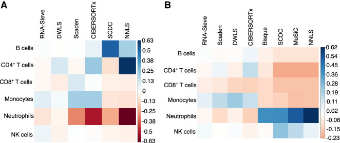
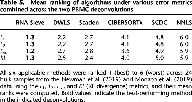
Subsequent deconvolutions showed that RNA-Sieve performed the best of all methods as measured by the mean absolute deviation (L₁ error) when aggregating across both analyses (Table 4). The presence of neutrophils presented a challenge for several methods, perhaps because they came from a different experiment or because of their uniquely low RNA counts. For example, in the bulk data from Newman et al. (2019) (Fig. 3A), neutrophils were strongly underestimated by CIBERSORTx, Scaden, and SCDC with most of that mass being allocated to either monocytes, CD4⁺ T cells, or B cells, respectively. RNA-Sieve and DWLS both performed well on these bulk samples, although RNA-Sieve slightly underestimated neutrophils in favor of monocytes and DWLS had minor difficulty distinguishing between CD4⁺ and CD8⁺ T cells. A similar story emerged for the Monaco et al. (2019) data (Fig. 3B), with CIBERSORTx, DWLS, Scaden, and, to a lesser extent, RNA-Sieve underestimating neutrophil and CD8⁺ T cell proportions while overweighting monocytes or CD4⁺ T cells. In contrast, Bisque, SCDC, and MuSiC strongly overweighted neutrophils (and sometimes natural killer cells) at the expense of other cell types. To produce a more formal and comprehensive comparison, we computed summary statistics in the same manner as Table 2 using the 24 bulk samples comprising the two data sets. RNA-Sieve achieves the best performance among all considered methods (Table 5) in each metric as it shows strong performance for both data sources. DWLS performs well on the Newman et al. data but fails to attain that level of accuracy on the Monaco et al. data.

Table 4.

Average L₁ errors with PBMC data and ground-truth cell proportions from flow cytometry

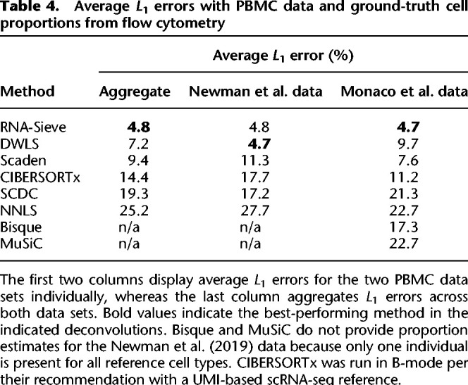
Figure 3.

Deconvolution biases for PBMC data with known ground-truth proportions. Average differences between inferred and true proportions were computed within each cell type across the 12 bulk samples present in each scenario. Consistent overestimation of a cell type's abundance results in darker blue squares, whereas red corresponds to chronic underestimation. Methods are ordered left to right by overall performance. (A) Deconvolution using Newman et al. (2019) data. (B) Deconvolution using Monaco et al. (2019) data.

Table 5.

Mean ranking of algorithms under various error metrics combined across the two PBMC deconvolutions

Keeping with the convention of several previous works, we also analyzed pancreatic islets data in which qualitative relationships between cell types are known rather than cell type proportions. RNA-Sieve is among the well-performing methods, and a full description can be found in Supplemental Text S1.2 and Supplemental Figure S8. A summary of runtimes for the different methods in these deconvolution tasks is available in Supplemental Text S1.3.

Analysis of real bulk organ samples

We next applied RNA-Sieve to real bulk RNA-seq data to analyze patterns in organ composition. We chose to continue working with the Tabula Muris Senis data set because it contains many bulk RNA-seq samples in addition to the scRNA-seq data previously described. Owing to its expansive experimental design across organs and ages, this resource is uniquely suited to interrogate changes in cell type compositions associated with the process of aging. In general, aging represents one of the more complicated biological processes, and one which occurs in every person or organism. Because of its ubiquity and significant effects on quality of life, improved understanding of the etiologies underlying age-associated functional deficits holds great potential therapeutic value, and we hope to identify changes in the balance of cell classes at different stages of life. Degradation of the musculoskeletal and immune systems are among the most apparent trends in mammalian aging. Here, we highlight results from three organs with roles in these bodily systems—the limb muscle in the former, and the spleen and bone marrow in the latter.

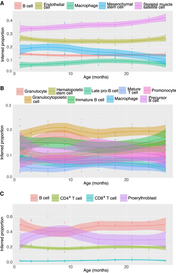
In limb muscle, we observed a noticeable increase in skeletal muscle satellite cells and a substantial decrease in the mesenchymal stem cell proportion in older mice (Fig. 4A). These trends are present, albeit fairly gradual, until around 21 mo old with more sudden changes apparent thereafter. There was also an apparent increase in macrophage proportions up until 15 mo of age, followed by a slow decline for the remainder of life. Each of these three cell types has been shown to function in muscle fiber repair through different mechanisms (Snijders et al. 2015). This pattern in cell type composition may thus indicate changes in the relative use of different regenerative pathways as individuals age.

Figure 4.

Deconvolution results for real bulks from the Tabula Muris Senis. Roughly 40 real bulk samples across 10 ages were deconvolved using RNA-Sieve in each of the limb muscle (A), bone marrow (B), and spleen (C). In all cases, Smart-seq2 data were used as the reference. Each point represents the inferred proportion for a given cell type in a bulk sample. Lines display the smoothed trend of proportions as a function of age, with uncertainty shown by the shaded intervals.

The rich combination of cell types present in the marrow, ranging from stem cells to more mature cell classes (Gurkan and Akkus 2008), yielded several age-associated trends in cell type composition (Fig. 4B), and we choose to focus on two. First, an effectively linear growth in the number of hematopoietic stem cells was observed with increasing age. Although this may seem surprising given reduced adaptive immunity with age, this exact phenomenon has been previously observed in both mice and humans (Pang et al. 2011), and it is accompanied by a decrease in functionality of these cells. Conversely, granulocyte proportion appeared to decrease after roughly 9 mo of age. Further examination reveals that the granulocyte fraction tends to mirror that of granulocytopoietic cells, but with an increasing deficit between the two as age increases. Such a pattern is suggestive of the reduced potency of granulocytopoiesis that we would expect with age. Hence, in the marrow we are able to identify known patterns of cell type composition variation despite the presence of many transcriptomically similar cell types.

The population of splenic immune cells primarily consists of B and T cells, with smaller quantities of other cell types (Hensel et al. 2019). Among these are different categories of progenitor cells, which are difficult to separate in their early stages, making it possible that several varieties are labeled together as proerythroblasts. We found that inferred proportions for B and T cells matched accepted ranges (Hensel et al. 2019) and noticed an unexpected and transient spike in the proportion of proerythroblasts peaking at roughly 9 mo of age (Fig. 4C). This increase is observed in all four of the 9-mo-old individuals and is thus not an artifact of outlying samples. Mice at this age are roughly analogous to humans of between 30 and 40 yr of age, and hematopoiesis is generally restricted to the marrow at this age except under stress conditions. This may indicate a programmed hematopoietic process or the behavior of a cell type not enumerated in the reference set and is a candidate for replication and follow-up.

Extension to confidence regions

The generative framework of RNA-Sieve permits extensions that remain out of reach using prior approaches to deconvolution. One such possibility is the computation of confidence regions for inferred cell type proportions. Despite its clear importance, error quantification in deconvolution is challenging and has received relatively scant attention, leaving users to only guess at the reliability of their results. Because deconvolution is sometimes performed upstream of tasks such as differential expression or eQTL detection, it is critical to understand the precision of estimated proportions. Because RNA-Sieve infers these proportions via maximum likelihood estimation, we can directly use the wide array of theory on asymptotic confidence bounds. Specifically, we construct confidence regions for inferred proportion values through numerical computation of the inverse empirical Godambe information matrix (see “Confidence intervals” in Methods). We show RNA-Sieve's ability to produce well-calibrated confidence regions in pseudobulk deconvolutions using Tabula Muris Senis data as well as with both real PBMC bulk data sets in “Validation with real bulk RNA-seq data.”

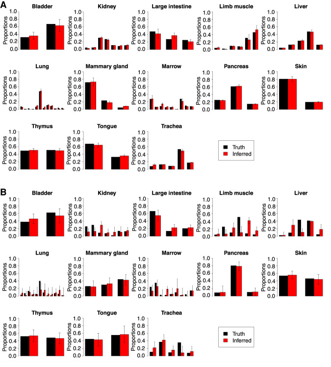
We began with within-protocol comparisons in which all modeling assumptions are generically met. As shown in Figure 5A and Supplemental Figure S9A, we obtain narrow, yet well-calibrated, confidence intervals. However, the typical deconvolution setting will present complications in the form of protocol differences in the scRNA-seq reference and bulk RNA-seq data. Under mild and plausible assumptions on these distributional shifts, our MLE framework is robust to such model misspecification (see “Confidence intervals”), and we still achieve good performance despite protocol mismatch (Fig. 5B; Supplemental Fig. S9B). Aggregating across runs, our 95%-confidence intervals contain the true cell type proportions 96.7% and 91.8% of the time in the within- and across-protocol deconvolutions, respectively.

Figure 5.

RNA-Sieve results with confidence intervals in pseudobulk experiments. Inferred cell type proportions in pseudobulk experiments using data from the Tabula Muris Senis experiment for within-protocol (Smart-seq2 for both reference and pseudobulk) (A) and across-protocol (Smart-seq2 reference and 10x Chromium pseudobulk) (B) experiments. The black error bars on inferred proportions show the marginal 95% confidence intervals computed from the estimated Godambe information produced by RNA-Sieve. See “Confidence intervals” for mathematical details. Supplemental Table S2 contains the cell types in each organ, which could not be displayed because of space constraints.

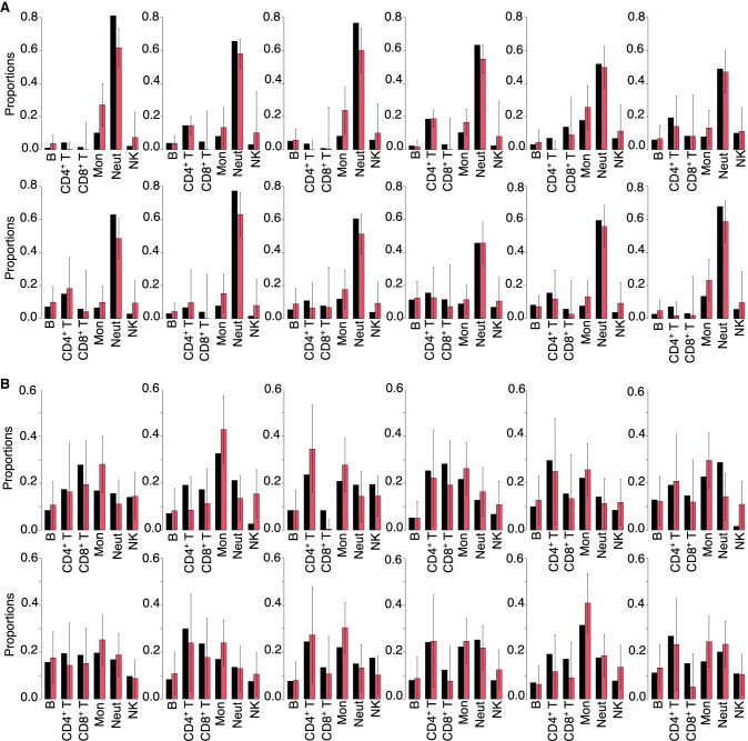
To ensure that we obtain sensible results with real bulk RNA-seq data, we also generated confidence intervals for the whole blood samples analyzed in “Validation with real bulk RNA-seq data.” We again obtain calibrated and sensible results, with our confidence intervals containing the truth 90.3% of the time in the Newman et al. (2019) bulk samples (Fig. 6A) and 95.8% of the time in the Monaco et al. (2019) bulk samples (Fig. 6B). Although assessing their accuracy is impossible absent ground-truth proportions, we also computed confidence intervals for the real bulks deconvolved in “Analysis of real bulk organ samples” to verify that RNA-Sieve's confidence intervals were reasonable in tissues besides whole blood. We found that these interval widths were similar to those we obtained in our other trials (Supplemental Fig. S10). The distributions of confidence interval half-widths for cell type proportions were also generally consistent across samples (Supplemental Fig. S11). We note that MuSiC presents a quantity that seemingly corresponds to the variance in proportion estimates, although it was not emphasized in their manuscript (Wang et al. 2019), and we generally found the produced values to be overly small in practice.

Figure 6.

RNA-Sieve results with confidence intervals for whole blood bulk samples with known cell type proportions. Inferred cell type proportions in deconvolutions using PBMC references and whole blood bulks as described in “Validation with real bulk RNA-seq data”: (A) Newman et al. (2019) data; (B) Monaco et al. (2019) data. True proportions as estimated by flow cytometry are in black, and RNA-Sieve's inferred proportions are in red. The black error bars on inferred proportions show the marginal 95% confidence intervals as produced by RNA-Sieve. Confidence intervals capture true proportions 90.3% and 95.8% of the time in the respective scenarios. See “Confidence intervals” for mathematical details.

In principle, confidence interval widths should depend on the number of cells and genes in the reference, the similarity among cell types in the reference, and the agreement between reference and bulk measurements. Our empirical results suggest that these factors indeed drive the widths of our intervals. For example, the confidence intervals in cross-protocol deconvolutions are wider than their within-protocol counterparts owing to our adaptive procedure's conservative nature when the reference and bulk measurements differ. This arises in part because we deem fewer genes reliable when compared to within-protocol experiments. Evidence of the contribution of reference sample size is present in a few organs, most notably the lung with its many low-frequency cell types.

Discussion

Here, we have introduced our method for supervised bulk gene expression deconvolution, RNA-Sieve, and illustrated its robust performance in a variety of settings. Unlike methods that rely on variants of least squares or the application of complex machine learning algorithms, we place the deconvolution problem into a generative probabilistic framework that models random noise in both the reference panel and bulk samples by relying on asymptotic theory. Through simulations and applications to real data, we showed the broad applicability of our method and its utility to investigate biological questions of interest.

It is valuable to understand how RNA-Sieve differs from other approaches and to consider the consequences of these divergent design choices. Least-squares-based solutions such as MuSiC (Wang et al. 2019), SCDC (Dong et al. 2021), and DWLS (Tsoucas et al. 2019) devise their own implementations of weighted non-negative least squares (W-NNLS). These methods aim to handle heteroskedasticity across genes by reweighting them according to their variability and specificity, allowing genes that are more informative to carry increased importance in the regression task. Alternatively, Bisque (Jew et al. 2020) uses NNLS after applying a transformation to bring the reference and bulk data into better distributional agreement. From a modeling perspective, least-squares-based solutions generally address uncertainty in the bulk, leaving stochasticity in the single-cell reference unaccounted for. Rather than devising a specialized gene-weighting scheme, RNA-Sieve naturally emphasizes some genes more than others via variances resulting from an explicit generative model incorporating noise in both single cells and the bulk. We also do not directly attempt to bring reference and bulk data into better agreement a là Bisque, instead filtering genes that display significant deviations from our assumptions. Integrating an explicit transformation remains an interesting possibility for RNA-Sieve. Other methods use machine learning techniques, such as CIBERSORTx (Newman et al. 2019), which uses ν-support vector regression, and Scaden (Menden et al. 2020), which uses deep neural networks. Despite continuing advances in explainability techniques, these approaches can be opaque to the user because of their reliance on high-complexity algorithms that often lack theoretical guarantees of optimality and provably accurate inference. Comparatively, our formulation of RNA-Sieve as the MLE of an explicit generative model is transparent in both parameter interpretation and performance guarantees. The parameters updated during optimization have explicit biological meanings and tracing their values allows for a deeper interrogation of the predictions RNA-Sieve generates. This is a useful feature when providing context to inferred cell type proportions as well as exploring the theoretical limits of deconvolution as a function of cell type properties. Like MuSiC, SCDC, Bisque, and Scaden, we do not select marker genes in RNA-Sieve. This helps us maintain computational efficiency while simultaneously providing robustness with respect to outlier fluctuations in gene expression. We also parallelize our optimization steps and jointly update parameters when deconvolving multiple bulk samples. This yields significant speedups relative to serial runs and allows us to share statistical strength across all bulks.

RNA-Sieve is embedded in a flexible generative framework, which can be adapted to a variety of situations to make deconvolution performance more effective. One of these is the modeling of further sources of variation. For instance, if gene expression distributions are expected to differ drastically across individuals from which samples are taken, this knowledge can be explicitly incorporated into our likelihood. Without such modification, RNA-Sieve implicitly follows the paradigm of MuSiC, SCDC, and Bisque in penalizing genes of large inter-individual variance via the marginal variances resulting from estimation of the reference panel. A similar notion applies to mitigating potential batch effects or effectively combining disparate references. Currently, different reference matrices that are believed to have the same expression distributions can be averaged together to increase statistical power without further modification of our present implementation.

A principal motivation of this work was to expand the scope of accessible questions in the deconvolution setting. Our likelihood-based approach facilitates extensions that are intractable with current algorithms. As a first step, we have chosen to show our ability to explicitly construct confidence regions for inferred proportions, producing a mathematically rigorous quantification of the uncertainty in our estimates. The necessity of these bounds is plainly substantiated by the use of deconvolution upstream of tasks ranging from cell type–specific differential expression to eQTL detection using heterogeneous RNA-seq organ samples. The credibility of any such analyses is predicated on the accuracy of deconvolution, because any errors in this initial step will propagate through to the final result. Consequently, we anticipate that our confidence regions will encourage improved assessment of the reliability of results obtained through these types of analyses. Our confidence intervals are also of obvious inherent value when using deconvolution results to infer differences in cell type composition between samples, whether a result of disease status or other factors. Beyond error quantification via confidence intervals, potent possibilities lie in hypothesis testing. Currently, CIBERSORTx does propose one type of test, although our understanding is that it tests whether any of the bulk cell types were found in the reference. This is rather restrictive, so we hope to develop procedures with broader utility. One example with clinical impact is a test to determine whether the reference panel is missing cell types present in the bulk sample. Although we have shown that RNA-Sieve is robust with respect to such misspecification (see “Performance in pseudobulk experiments”), it is nonetheless beneficial to know whether the deconvolution performed was sufficiently valid using a principled approach. Such a test can be directly developed in our framework by examining the residuals produced by our maximum likelihood estimate, and work in this direction is underway.

Despite the flurry of recently developed methods, the question of statistical deconvolution of gene expression data remains far from solved. RNA-Sieve illustrates the efficacy, adaptability, as well as promise of generative modeling in this setting, and we hope it spurs continued development within other methodological paradigms. In particular, notions of error quantification and hypothesis testing merit further attention.

Methods

Here, we present the mathematical details of RNA-Sieve. For the reader interested in high-level guidance on the use RNA-Sieve and preprocessing steps, we compiled Supplemental Table S3 as an overview.

Notation

To ease the parsing of equations, we introduce our notation here. We generally refer to vector quantities with boldfaced lowercase letters, and plain lowercase and uppercase symbols are reserved for scalars (or scalar functions) and matrices, respectively. The kth column vector of a matrix A = (a_ij)_ij is written as a_k, and inner products between vectors v, w are typically denoted $\langle \mathit{v},\mathit{w}\rangle$. To distinguish observed, random quantities from the underlying deterministic, ground-truth objects, we add tildes to the former and asterisks to the latter; for example, $\tilde{\mathit{b}}$ are observed bulk gene expressions and b* are the true bulk gene expression means. Estimates of latent parameters carry hats; for example, $\hat{\mathit{\alpha }}$ is the vector of mixture weights inferred by our deconvolution procedure. Finally, we denote by [n] the set of n elements {1, …, n}, and by ${\mathrm{\Delta }}^{K-1}=\{x\in {\mathbb{R}}^K:\parallel x{\parallel }_1=1\mathrm{and}{x}_k\ge 0\mathrm{for}\mathrm{all}k\}$ the K − 1 dimensional simplex.

Mathematical model

We assume that for each gene g ∈ [G] and cell type k ∈ [K], there exists a distribution ν_g,k describing the expression of gene g in cell type k. Because multiple cell types compose any given organ, the expression of gene g in a cell drawn at random from an organ is governed by the mixture distribution

$${\rho }_g=\sum _{k=1}^K{\alpha }_k^{\ast }{\nu }_{g,k},$$ (2)

where ${\mathit{\alpha }}^{\ast }={\left({\alpha }_k^{\ast }\right)}_{k\in \left[K\right]}\in {\mathrm{\Delta }}^{K-1}$ contains the proportions of each cell type in the organ of interest. Despite the a priori infinite-dimensional setting, if G > K and ρ_g, {ν_g,k}_k∈[K] are fully known and sufficiently distinct, the convex combination of Equation 2 immediately implies that α* can be recovered as the unique solution of the finite-dimensional problem

$$\underset{M}{\underbrace{\left[\begin{array}{ccc}f\left({\nu }_{1,1}\right)& \dots & f\left({\nu }_{1,K}\right)\\ ⋮& ⋮& ⋮\\ f\left({\nu }_{G,1}\right)& \dots & f\left({\nu }_{G,K}\right)\end{array}\right]}}\cdot \underset{\mathit{\alpha }}{\underbrace{\left[\begin{array}{c}{\alpha }_1\\ ⋮\\ {\alpha }_K\end{array}\right]}}=\underset{\mathit{b}}{\underbrace{\left[\begin{array}{c}f\left({\rho }_1\right)\\ ⋮\\ f\left({\rho }_G\right)\end{array}\right]}},$$ (3)

where f is any suitable linear function on the space of probability distributions on ℝ (i.e., $f(\sum _j{w}_j{\mu }_j)=\sum _j{w}_{j}f({\mu }_j)$ for any convex combination of distributions μ_j). Natural f to consider include point evaluations at x ∈ ℝ; that is, $f\left(\nu \right)=F_{\nu }\left(x\right)$, where $F_{\nu }$ denotes the cumulative distribution function (CDF) of ν, or its ith moments $f(\nu )=\int x^i\nu (dx)$, both of which enjoy a wealth of statistical theory and proposed estimators. In experimental settings, exact gene expression distributions are not accessible and must be estimated, so utilizing easily and robustly inferable f is crucial. In addition to a lack of direct access to {ρ_g}_g∈[G], any analysis is further complicated by the fact that bulk sequencing only yields gene expression levels over whole samples and not for particular cells or cell types. That is, the output is effectively a random variable $X_g=\sum _{i=1}^n{X}_{g,i}$ where $X_{g,i}\stackrel{iid}{\sim }{\rho }_g$, which gives the measured expression of gene g aggregated over the n ∈ ℕ individual cells composing the sample. It is thus expedient to choose an f in Equation 3 that is not only linear on the space of probability distributions, but also for sums of random variables. The essentially unique such f is the expectation f(ν) = $\mathbb{E}$_X∼ν X, which turns Equation 3 into

$$M\mathit{\alpha }=\frac{\mathit{b}}{n},\mathrm{where}{m}_{g,k}={\mathbb{E}}_{Y\sim {\nu }_{g,k}}Y\mathrm{and}{b}_g=\mathbb{E}{X}_g.$$ (4)

Incorporating the fact that we only observe noisy bulk samples X_g instead of b_g directly results in

$$\frac{\tilde{\mathit{b}}}{n}=\frac{\left(\mathit{b}+{\epsilon }_{\mathit{b}}\right)}{n}=M\mathit{\alpha }+\frac{{\epsilon }_{\mathit{b}}}{n},$$ (5)

where ${({\epsilon }_{\mathit{b}})}_g\sim X_g-b_g=\sum _{i=1}^n(X_{g,i}-b_g/n)\sim \mathcal{N}(0,n\cdot {\sigma }_g^2(M,\mathit{\alpha },S))$ for large n by the central limit theorem (CLT), with ${\sigma }_g^2(M,\mathit{\alpha },S):=\mathrm{Var}({\rho }_g)$ as a function of M, α, and S = (s_g,k)_g,k := Var(ν_g,k).

Incorporating the dependence of ${\sigma }_g^2$ on α

If the dependence of ${\sigma }_g^2$ on α is ignored, Equation 5 lends itself to a simple (weighted) non-negative least-squares scheme solving

$$M\mathit{\alpha }=\frac{\tilde{\mathit{b}}}{n}.$$ (6)

This yields a solution ${\hat{\mathit{\alpha }}}_{LS}$ with $\parallel {\hat{\mathit{\alpha }}}_{LS}{\parallel }_1\approx 1$ that simply requires rescaling to fit onto the simplex. This together with data-driven modifications is the approach pursued in Dong et al. (2021), Tsoucas et al. (2019), and Wang et al. (2019), where it is argued that Equation 6 outperforms previous methods.

The first improvement of RNA-Sieve over prior approaches stems from explicitly incorporating the dependence of ${\sigma }_g^2$ on α. More concretely, we compute

$$\begin{array}{rl}{\sigma }_g^2={\sigma }_g^2(M,\mathit{\alpha },S)& =\mathrm{Var}({\rho }_g)={\mathbb{E}}_{X\sim {\rho }_g}{X}^2-{({\mathbb{E}}_{X\sim {\rho }_g}X)}^2\\ & =(\sum _{k=1}^K{\alpha }_k^{\ast }{\mathbb{E}}_{Y\sim {\nu }_{g,k}}{Y}^2)-b_g^2\\ & =(\sum _{k=1}^K{\alpha }_k^{\ast }[s_{g,k}+m_{g,k}^2])-b_g^2.\end{array}$$ (7)

The likelihood of observing data $\tilde{\mathit{b}}$ then follows from the central limit theorem:

$${\mathbb{P}}_{M,S}^{\mathit{\alpha },n}(\tilde{\mathit{b}}\in d\mathit{p})=\prod _{g=1}^G\frac{1}{\sqrt{2\pi n{\sigma }_g^2(M,\mathit{\alpha },S)}}\exp \left\{\frac{-{\left[p_g-n{(M\mathit{\alpha })}_g\right]}^2}{2n{\sigma }_g^2(M,\mathit{\alpha },S)}\right\}.$$ (8)

Accounting for uncertainty in the design matrix

The preceding assumes exact knowledge of the individual distributions ν_g,k (or rather their expectations m_g,k), which is implausible in experimental settings. Instead, M needs to be estimated from data through some estimator $\tilde{M}$, which we conveniently take to be the sample mean of expression across cells within each cell type, ${\tilde{m}}_{g,k}={\displaystyle \frac{1}{c_k}\sum _{i=1}^{c_k}{C}_{g,k}^i}$, where $C_{g,k}^i\stackrel{iid}{\sim }{\nu }_{g,k}$, and c_k denotes the number of single cells of cell type k. With this additional correction, Equation 5 becomes

$$\frac{\tilde{\mathit{b}}}{n}=\tilde{M}\mathit{\alpha }+\frac{{\epsilon }_{\mathit{b}}}{n}\mathrm{and}\tilde{M}=M+{\epsilon }_M$$ (9)

where ɛ_M is a matrix of entries (ɛ_M)_g,k independently following $\mathcal{N}\left(0,s_{g,k}/c_k\right)$ distributions. The second major difference between RNA-Sieve and existing tools, especially those based on least-squares methods, is the correction of the least-squares-type likelihood (Equation 8) by this stochasticity in the design matrix:

$$\begin{array}{rl}{\mathbb{P}}_{M,S}^{\mathit{\alpha },n,\mathit{c}}\left(\tilde{\mathit{b}}\in d\mathit{p},\tilde{M}\in dO\right)& =\prod _{g=1}^G\frac{1}{\sqrt{2\pi n{\sigma }_g^2(M,\mathit{\alpha },S)}}\exp \left\{\frac{-{[p_g-n{\left(M\mathit{\alpha }\right)}_g]}^2}{2n{\sigma }_g^2(M,\mathit{\alpha },S)}\right\}\\ & \times \prod _{g\in \left[G\right],k\in \left[K\right]}\frac{1}{\sqrt{2\pi s_{g,k}/c_k}}\exp \left\{\frac{-{(o_{g,k}-m_{g,k})}^2}{2s_{g,k}/c_k}\right\}.\end{array}$$ (10)

Our method uses the likelihood shown in Equation 10, the suitability of which depends on a few implicit assumptions that are worth examining. The first is that the large number of cells assayed in an experiment permits us to use asymptotic theory and apply the classical CLT. As a result, we can write down a likelihood for our observations using normal distributions as long as Var(ν_g,k) < ∞, which is true because gene expression profiles are necessarily bounded. Second, we suppose that the errors arising from estimating b and M are independent. This is appropriate because the bulk and single-cell experiments are performed separately. We additionally presume that expression levels in different genes are independent, as are those in different cells. It is unclear whether the latter is completely true in practice, although there is little evidence to the contrary. On the other hand, expression levels across genes within samples (either bulk or individual cells) are liable to be somewhat dependent owing to expression coregulation and the nature of the sampling process performed in RNA-seq. Given the large number of genes assayed, the latter codependence is apt to be fairly small. Meanwhile, coexpression estimation in single cells remains an open problem independent of deconvolution tasks, and so is not accounted for in RNA-Sieve. Once correlation structure is known, however, it may be incorporated into our proposed likelihood. Last, the parameter n is meaningful in within-protocol deconvolutions but may require additional interpretation in cross-protocol settings. A discussion can be found in Supplemental Text S1.4 and Supplemental Figure S12.

Joint deconvolution of multiple bulk samples

If it is known that multiple bulk gene expression vectors share the same constituent cell type expression profiles, we can gain statistical strength and decrease the computational burden by inferring their mixture proportions jointly rather than individually. Assuming statistical independence of the bulk sample observations, we simply augment the likelihood in Equation 10 by including the N − 1 additional mixtures in $A=\left({\mathit{\alpha }}_1,\dots ,{\mathit{\alpha }}_N\right)\in {\mathbb{R}}^{K\times N},\tilde{B}=\left({\tilde{\mathit{b}}}_1,\dots ,{\tilde{\mathit{b}}}_N\right)\in {\mathbb{R}}^{G\times N}$ and n = (n₁, …, n_N):

$$\begin{array}{rl}{\mathbb{P}}_{M,S}^{\mathit{\alpha },\mathbf{n},\mathit{c}}(\tilde{B}\in dP,\tilde{M}\in dO)& =\prod _{b=1}^N\prod _{g=1}^G\frac{1}{\sqrt{2\pi n_b{\sigma }_g^2(M,{\mathit{\alpha }}_b,S)}}\exp \left\{\frac{-{[{\left({\mathit{p}}_b\right)}_g-n_b{\left(M{\mathit{\alpha }}_b\right)}_g]}^2}{2n_b{\sigma }_g^2(M,{\mathit{\alpha }}_b,S)}\right\}\\ & \times \prod _{g\in \left[G\right],k\in \left[K\right]}\frac{1}{\sqrt{2\pi s_{g,k}/c_k}}\exp \left\{\frac{-{(o_{g,k}-m_{g,k})}^2}{2s_{g,k}/c_k}\right\}.\end{array}$$ (11)

The resultant increase in power depends solely on the statistical independence of distinct bulk samples rather than their respective cell type compositions. In fact, samples of dissimilar compositions are preferable because they provide nonredundant information. Conversely, bulk samples exhibiting heterogeneity in gene expression patterns (e.g., through differential expression) without corresponding reference matrices M amount to model misspecification, and thus may negatively impact inference. This impediment is a mathematically unavoidable challenge for all deconvolution methods. In our particular applications, we did not find a strong effect of sample heterogeneity on our results; for instance, simultaneous deconvolution with mice of different ages yielded highly similar results as when we stratified by age. In the case of cell types with strong expression differences across different phenotypes, this may not hold, however.

Data pre-processing procedure

Beyond a simple, largely standard cell filtering and normalization scheme (Supplemental Text S1.5), we implemented two additional gene filtering steps that improve robustness to cross-protocol differences in gene expression measurements. The motivation behind these steps is as follows:

1. As a convex combination of expression levels from different cell types (under our generative model [Equation 10]), a gene's true expression b_g must lie between its smallest and largest corresponding expressions m_g,k across cell types k ∈ [K], which naturally motivates a filtering scheme based on violations of these constraints. Of course, these inequalities do not necessarily hold in the presence of observational noise, which may push a gene's bulk expression outside of its theoretical extremes. However, a stochastic version exists in which

   $${\mathbb{P}}_{M,S}^{\mathit{\alpha },n,\mathit{c}}[\delta ({\tilde{b}}_g,[\underset{k\in [K]}{min}{\tilde{m}}_{g,k},\underset{k\in [K]}{max}{\tilde{m}}_{g,k}])\ge t]$$ (12)

   decays in t with sub-Gaussian tails (with constants depending on {σ_g,k}_k∈[K]), where $\delta \left(p,A\right)=\underset{a\in A}{inf}\left|p-a\right|$ is the shortest distance of the point p to a set A. It is thus plausible to filter out all genes for which Equation 12 is sufficiently small (in principle, computing the precise tail bounds [Equation 12] requires access to the true parameter α, which before deconvolution is not available; however, reasonable upper bounds of Equation 12 can be calculated independently of α).
2. Gene expression profiles often experience shifts when measured with distinct protocols. For example, mean and variance estimates of some gene expression levels may correlate little, or even not at all, across data generated using Smart-seq2, UMI-based, or bulk RNA-seq technologies. To identify and remove these genes, we resort to a handful of empirically effective filtering steps. Specifically, we remove a gene if it presents as an outlier (as measured by median absolute deviations from the median) in any of the following summary statistics:

   $$\begin{array}{cc}{T}_M(g)=\underset{k\in [K]}{max}{\hat{m}}_{g,k},& T_S(g)=\underset{k\in \left[K\right]}{max}{\hat{s}}_{g,k},\\ R_{S/M}(g)=\underset{k\in \left[K\right]}{max}\frac{{\hat{s}}_{g,k}^{\frac{1}{2}}}{{\hat{m}}_{g,k}}=\underset{k\in \left[K\right]}{max}{c}_V(C_{g,k}),& R_{b/M}(g)=\underset{k\in \left[K\right]}{min}\frac{{\hat{b}}_g}{{\hat{m}}_{g,k}},\end{array}$$ (13)

   where c_V (C_g,k) denotes the coefficient of variation associated with expression profiles of gene g in cell type k. Although the choice of these summary statistics was primarily guided by empirical considerations, they do reveal intuitively plausible and previously observed patterns: T_M, T_S, and R_S/M reflect the fact that severe overexpression or underexpression, or high degrees of variability in expression are not well-preserved across protocols, whereas $R_{b/M}(g)={\hat{b}}_g/{max}_{k\in \left[K\right]}{\hat{m}}_{g,k}$ directly assesses any abnormal conversion factors between bulk and reference protocols.

In our experience, applying these filters based on Equations 12 and 13 on top of the basic cell filter retains between 3000 − 12,000 genes on which to perform deconvolution.

Optimization and estimation

We estimate α, the cell type proportions for a given bulk sample, using the MLE that arises from maximizing Equation 10. Given the number of free parameters (GK + K in total, corresponding to M, α, and n) and structure of the likelihood, this is nontrivial, with standard optimization schemes commonly failing or returning suboptimal solutions. On its face, the shape of Equation 10 is reminiscent of loss functions appearing in so-called total least-squares formulations, for example in Golub and Van Loan (1980), whose minimizers can typically be found through SVD-based solutions. However, entry-wise uncertainties ɛ_M and the dependence of ɛ_b on α render such spectral tools inapplicable to our setting; indeed, the corresponding linear algebraic problem consists of finding low-rank approximations to the concatenation of M and b in a Frobenius norm with α-dependent weights, for which no satisfactory theory exists. We thus propose an alternating maximization scheme that iteratively estimates and updates α, M, and n (and consequently ${\sigma }_g^2$) via a combination of quadratic programming and gradient descent. Despite the increased computational burden relative to W-NNLS or similar techniques, we find that convergence times remain reasonable, requiring between 15 and 40 min on typical data sets of 10,000 + genes and six cell types using a modern laptop computer. We sketch an overview of our optimization procedure below in Algorithm 1 (where ${\mathbb{P}}_{M,S\mid {\mathit{\sigma }}^2\left(M^{\mathrm{\prime }},{\mathit{\alpha }}^{\mathrm{\prime }},S\right)}^{\mathit{\alpha },n,\mathit{c}}$ refers to Equation 10 with σ² (M, α, S) kept fixed at σ² (M^′, α^′, S)).

Algorithm 1: Find MLE of α —

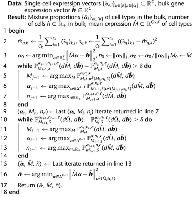
Implementations of Algorithm 1 are currently available in Python and Mathematica. Both use standard design choices when implementing MLEs (for details, see Supplemental Text S1.6).

Confidence intervals

As indicated in “Extension to confidence regions,” the explicit generative modeling of Equation 10 allows us to not only compute precise point estimators of α and n, but also to quantify this precision through confidence regions. More concretely, because our model is well-behaved in the sense of satisfying all assumptions in, for example, Theorem 9.14 of Keener (2011), we expect our estimates $\hat{\mathit{\alpha }}$ and $\hat{n}$ to be distributed normally around the true configuration α*, n* with covariance matrix given by the inverse of the Fisher information $I_{M,S}^{\mathit{c}}({\mathit{\alpha }}^{\ast },n^{\ast })\approx I_{\hat{M},S}^{\mathit{c}}(\hat{\mathit{\alpha }},\hat{n})$. Given such asymptotic normality, it is straightforward to construct both marginal confidence intervals (from the diagonal entries of ${[I_{\hat{M},S}^{\mathit{c}}]}^{-1}$) and K-dimensional confidence regions around $\hat{\mathit{\alpha }}$. Generically, there are infinitely many possibilities for choosing such confidence regions from $I_{\hat{M},S}^{\mathit{c}}(\hat{\mathit{\alpha }},\hat{n})$, so we provide the entire (inverse) Fisher information to the user to allow computation of their preferred confidence volume. One option is the canonical (i.e., Lebesgue volume-minimizing) q-confidence region $C_q=\{\mathit{\alpha }\in {\mathbb{R}}_{+}^{K-1}:\sum _{k=1}^{K-1}{a}_k\le 1,\parallel \mathit{\alpha }-\hat{\mathit{\alpha }}{\parallel }_{I_{\hat{M},S}^{\mathit{c}}}^2\le F_{{\chi }_{K-1}^2}^{-1}(q)\}$, where ${\parallel \mathit{v}\parallel }_{\mathrm{\Sigma }}=\langle \mathit{v},{\mathrm{\Sigma }}^{-1}\mathit{v}\rangle$ is the Mahalanobis norm of v associated with covariance matrix Σ, $F_{{\chi }_{K-1}^2}$ denotes the CDF of a χ² variable with K − 1 degrees of freedom, and where we reparameterize α to account for the simplex constraint in our computation of the Fisher information matrix; we compute this option by default.

Confidence intervals derived in this manner are, as a consequence of the aforementioned Theorem 9.14 in Keener (2011), necessarily well-calibrated if data adhere to our generative model (Equation 10). As observed in “Data pre-processing procedure,” this may not hold when protocol differences in the reference and bulk experiments induce significant distributional shifts. Nonetheless, we can still provide conservative, yet well-calibrated, confidence regions by generalizing the Fisher information $I_{\hat{M},S}^{\mathit{c}}(\hat{\mathit{\alpha }},\hat{n})$ to the Godambe information matrix $G_{\hat{M},S}^{\mathit{c}}(\hat{\mathit{\alpha }},\hat{n})$ of the data (Godambe 1960). If protocol mismatches result in the true generating distribution ℚ of the data not lying within our model family $\mathcal{M}={\{{\mathbb{P}}_{M,S}^{\mathit{\alpha },n,\mathit{c}}\}}_{(M,\mathit{\alpha },n)\in \mathrm{\Theta }}$, where Θ ⊂ ℝ^{G·K+(K−1)+1} is the space of all possible parameter configurations, then $G_{\hat{M},S}^{\mathit{c}}(\hat{\mathit{\alpha }},\hat{n})$ describes the Gaussian fluctuations of $(\hat{\mathit{\alpha }},\hat{n})$ around the KL-projection of ℚ onto $\mathcal{M}$; that is, $({\mathit{\alpha }}^{\pi },n^{\pi },M^{\pi })=\arg \underset{(\mathit{\alpha },n,M)\in \mathrm{\Theta }}{min}KL(\mathbb{Q}\parallel {\mathbb{P}}_{M,S}^{\mathit{\alpha },n,\mathit{c}})$, where $KL(\nu \parallel \mu )$ denotes the Kullback-Leibler between two probability distributions ν and μ. Thus confidence regions for $\hat{\mathit{\alpha }}$ based on $G_{\hat{M},S}^{\mathit{c}}(\hat{\mathit{\alpha }},\hat{n})$ are still well-calibrated, assuming that ${\mathit{\alpha }}^{\ast }\approx {\mathit{\alpha }}^{\pi }$, which is plausible given that distributional shifts induced by protocol differences appear to affect expression means (the entries of M) primarily through global scaling. In the absence of distributional mismatches, the Godambe information matrix $G_{\hat{M},S}^{\mathit{c}}(\hat{\mathit{\alpha }},\hat{n})$ collapses to the (empirical) Fisher information matrix $I_{\hat{M},S}^{\mathit{c}}(\hat{\mathit{\alpha }},\hat{n})$, and our confidence region estimation proceeds through $G_{\hat{M},S}^{\mathit{c}}(\hat{\mathit{\alpha }},\hat{n})$ in both within- and cross-protocol settings by default, although the user may still choose the more conservative option. Occasionally, especially when constituent cell types are closely related to each other, the resulting covariance matrices may be nearly singular, making their inversion computationally difficult. To overcome potential numerical instabilities, we subsample genes based on their residual values. This reduces the probability of collinearities and produces more well-behaved confidence intervals. Simulations both across and within protocols confirm the utility of our confidence regions, and therefore the validity of the ${\mathit{\alpha }}^{\pi }\approx {\mathit{\alpha }}^{\ast }$ assumption, assessed in this manner (cf. Fig. 5).

Benchmarking procedures

We used two distinct approaches to benchmark computational deconvolution methods. The first, performing “pseudobulk” experiments, is a common strategy that aggregates scRNA-seq measurements across cells to construct gene expression mixtures with known cell type proportions. For this task, we used data from the Tabula Muris Senis Consortium, which covers many organs/tissues and cell types in two different single-cell experimental protocols: Smart-seq2 and 10x Genomics Chromium. Specifically, we used bladder, kidney, large intestine, limb muscle, liver, lung, mammary gland, marrow, pancreas, skin, thymus, tongue, and trachea in these in silico experiments (Supplemental Table S2). For each tissue, four different deconvolutions were performed. For cross-protocol deconvolutions, one in which the reference came from Smart-seq2 data with 10x Chromium pseudobulk and one in the reverse configuration. For within-protocol deconvolutions, the reference and pseudobulk were built using (nonoverlapping) cells from the same protocol. For all pseudobulk deconvolution scenarios, a single reference set and pseudobulk was constructed. All eligible cells from each protocol were used. For scRNA-seq data from Tabula Muris Senis, the cell filtering procedure described in “Data pre-processing procedure” was applied.

Our second approach exploited the availability of bulk RNA-seq data sets with known cell type proportions. For the PBMC and neutrophil scRNA-seq data sets, cells were filtered after manual inspection. Owing to the large number of neutrophils available, 250 cells were randomly sampled from one individual for use with the Newman et al. (2019) reference and 1250 across three individuals were randomly sampled for use with the 10x Genomics reference. We considered four different scenarios:

1. Breast cancer and fibroblast cell lines and mixture from Dong et al. (2021);

2. Reference PBMCs and neutrophils from Newman et al. (2019) and Xie et al. (2020), respectively, with bulk whole blood from Newman et al. (2019);

3. Reference PBMCs and neutrophils from 10x Genomics and Xie et al. (2020), respectively, with bulk whole blood from Monaco et al. (2019); and

4. Pancreatic islets from Xin et al. (2016) and Fadista et al. (2014).

The same data were used for all algorithms in each deconvolution, and all were run as described in their respective tutorials using default settings unless otherwise noted. When MuSiC was run, NNLS results were taken from MuSiC's implementation; otherwise, the DWLS implementation was used. The corresponding scRNA-seq and bulk RNA-seq data files are available at the Song Laboratory GitHub repository (https://github.com/songlab-cal/rna-sieve).

We used the L₁, L₂, and L_∞ distances, in addition to the Kullback-Leibler (KL) divergence, as our performance metrics for their ease of interpretation and ability to capture different aspects of algorithm performance. Whereas the L₁ and L₂ distances, which we further average across cell types, relate to common error notions such as the mean absolute deviation and root-mean-square error, the L_∞ distance measures the largest difference between true and inferred values across all cell types and quantifies the worst-case performance in a deconvolution task. The KL divergence is a popular manner by which to compare probability distributions and naturally applies to the interpretation of cell type proportions as sampling probabilities for an individual cell. It is also more sensitive to rarer cell types than the other considered metrics. We compute $KL(\hat{\mathit{\alpha }}\parallel {\mathit{\alpha }}^{\ast })$ rather than $KL({\mathit{\alpha }}^{\ast }\parallel \hat{\mathit{\alpha }})$ because it corresponds to the false positive rate when testing H₀ :α = α* against $H_1:\mathit{\alpha }=\hat{\mathit{\alpha }}$ through a likelihood ratio test, making it more relevant.

Data sets

All data used are publicly available and described in Supplemental Table S4, with accession numbers included.

Software availability

RNA-Sieve is implemented in both Python and Mathematica and is provided as Supplemental Code. For the most recent version of the software, please visit the Song Laboratory GitHub repository (https://github.com/songlab-cal/rna-sieve).

Competing interest statement

The authors declare no competing interests.

References

- Avila Cobos F, Vandesompele J, Mestdagh P, De Preter K. 2018. Computational deconvolution of transcriptomics data from mixed cell populations. Bioinformatics 34: 1969–1979. 10.1093/bioinformatics/bty019 [DOI] [PubMed] [Google Scholar]
- Bense RD, Sotiriou C, Piccart-Gebhart MJ, Haanen JB, van Vugt MA, de Vries EG, Schröder CP, Fehrmann RS. 2017. Relevance of tumor-infiltrating immune cell composition and functionality for disease outcome in breast cancer. J Natl Cancer Inst 109: djw192. 10.1093/jnci/djw192 [DOI] [PMC free article] [PubMed] [Google Scholar]
- Bremnes RM, Busund LT, Kilvær TL, Andersen S, Richardsen E, Paulsen EE, Hald S, Khanehkenari MR, Cooper WA, Kao SC, et al. 2016. The role of tumor-infiltrating lymphocytes in development, progression, and prognosis of non–small cell lung cancer. J Thorac Oncol 11: 789–800. 10.1016/j.jtho.2016.01.015 [DOI] [PubMed] [Google Scholar]
- Cabrera O, Berman DM, Kenyon NS, Ricordi C, Berggren PO, Caicedo A. 2006. The unique cytoarchitecture of human pancreatic islets has implications for islet cell function. Proc Natl Acad Sci 103: 2334–2339. 10.1073/pnas.0510790103 [DOI] [PMC free article] [PubMed] [Google Scholar]
- Dong M, Thennavan A, Urrutia E, Li Y, Perou CM, Zou F, Jiang Y. 2021. SCDC: bulk gene expression deconvolution by multiple single-cell RNA sequencing references. Brief Bioinform 22: 416–427. 10.1093/bib/bbz166 [DOI] [PMC free article] [PubMed] [Google Scholar]
- Fadista J, Vikman P, Laakso EO, Mollet IG, Esguerra JL, Taneera J, Storm P, Osmark P, Ladenvall C, Prasad RB, et al. 2014. Global genomic and transcriptomic analysis of human pancreatic islets reveals novel genes influencing glucose metabolism. Proc Natl Acad Sci 111: 13924–13929. 10.1073/pnas.1402665111 [DOI] [PMC free article] [PubMed] [Google Scholar]
- Funada Y, Noguchi T, Kikuchi R, Takeno S, Uchida Y, Gabbert HE. 2003. Prognostic significance of CD8+ T cell and macrophage peritumoral infiltration in colorectal cancer. Oncol Rep 10: 309–313. 10.3892/or.10.2.309 [DOI] [PubMed] [Google Scholar]
- Godambe VP. 1960. An optimum property of regular maximum likelihood estimation. Ann Math Statist 31: 1208–1211. 10.1214/aoms/1177705693 [DOI] [Google Scholar]
- Goldman SL, MacKay M, Afshinnekoo E, Melnick AM, Wu S, Mason CE. 2019. The impact of heterogeneity on single-cell sequencing. Front Genet 10: 8. 10.3389/fgene.2019.00008 [DOI] [PMC free article] [PubMed] [Google Scholar]
- Golub GH, Van Loan CF. 1980. An analysis of the total least squares problem. SIAM J Numer Anal 17: 883–893. 10.1137/0717073 [DOI] [Google Scholar]
- Gurkan UA, Akkus O. 2008. The mechanical environment of bone marrow: a review. Ann Biomed Eng 36: 1978–1991. 10.1007/s10439-008-9577-x [DOI] [PubMed] [Google Scholar]
- Hagenauer MH, Schulmann A, Li JZ, Vawter MP, Walsh DM, Thompson RC, Turner CA, Bunney WE, Myers RM, Barchas JD, et al. 2018. Inference of cell type content from human brain transcriptomic datasets illuminates the effects of age, manner of death, dissection, and psychiatric diagnosis. PLoS One 13: e0200003. 10.1371/journal.pone.0200003 [DOI] [PMC free article] [PubMed] [Google Scholar]
- Hensel JA, Khattar V, Ponnazhagan S. 2019. Characterization of immune cell subtypes in three commonly used mouse strains reveals gender and strain-specific variations. Lab Invest 99: 93–106. 10.1038/s41374-018-0137-1 [DOI] [PMC free article] [PubMed] [Google Scholar]
- Hu P, Fabyanic E, Kwon DY, Tang S, Zhou Z, Wu H. 2017. Dissecting cell-type composition and activity-dependent transcriptional state in mammalian brains by massively parallel single-nucleus RNA-seq. Mol Cell 68: 1006–1015.e7. 10.1016/j.molcel.2017.11.017 [DOI] [PMC free article] [PubMed] [Google Scholar]
- Jew B, Alvarez M, Rahmani E, Miao Z, Ko A, Garske KM, Sul JH, Pietiläinen KH, Pajukanta P, Halperin E, et al. 2020. Accurate estimation of cell composition in bulk expression through robust integration of single-cell information. Nat Commun 11: 1971. 10.1038/s41467-020-15816-6 [DOI] [PMC free article] [PubMed] [Google Scholar]
- Kalisky T, Rajendran PS, Sahoo D, Sim S, Okamoto J, Miranda SP, Johnston DM, Clarke MF, Quake SR, Dalerba P, et al. 2013. Analysis of human colon tissue cell composition using single-cell gene-expression PCR. J Biomol Tech 24: S11. [Google Scholar]
- Keener RW. 2011. Theoretical statistics: topics for a core course. Springer, New York. [Google Scholar]
- Lowe R, Rakyan VK. 2014. Correcting for cell-type composition bias in epigenome-wide association studies. Genome Med 6: 23. 10.1186/gm540 [DOI] [PMC free article] [PubMed] [Google Scholar]
- Melé M, Ferreira PG, Reverter F, DeLuca DS, Monlong J, Sammeth M, Young TR, Goldmann JM, Pervouchine DD, Sullivan TJ, et al. 2015. The human transcriptome across tissues and individuals. Science 348: 660–665. 10.1126/science.aaa0355 [DOI] [PMC free article] [PubMed] [Google Scholar]
- Menden K, Marouf M, Oller S, Dalmia A, Magruder DS, Kloiber K, Heutink P, Bonn S. 2020. Deep learning–based cell composition analysis from tissue expression profiles. Sci Adv 6: eaba2619. 10.1126/sciadv.aba2619 [DOI] [PMC free article] [PubMed] [Google Scholar]
- Monaco G, Lee B, Xu W, Mustafah S, Hwang YY, Carre C, Burdin N, Visan L, Ceccarelli M, Poidinger M, et al. 2019. RNA-seq signatures normalized by mRNA abundance allow absolute deconvolution of human immune cell types. Cell Rep 26: 1627–1640.e7. 10.1016/j.celrep.2019.01.041 [DOI] [PMC free article] [PubMed] [Google Scholar]
- Newman AM, Steen CB, Liu CL, Gentles AJ, Chaudhuri AA, Scherer F, Khodadoust MS, Esfahani MS, Luca BA, Steiner D, et al. 2019. Determining cell type abundance and expression from bulk tissues with digital cytometry. Nat Biotechnol 37: 773–782. 10.1038/s41587-019-0114-2 [DOI] [PMC free article] [PubMed] [Google Scholar]
- Pang WW, Price EA, Sahoo D, Beerman I, Maloney WJ, Rossi DJ, Schrier SL, Weissman IL. 2011. Human bone marrow hematopoietic stem cells are increased in frequency and myeloid-biased with age. Proc Natl Acad Sci 108: 20012–20017. 10.1073/pnas.1116110108 [DOI] [PMC free article] [PubMed] [Google Scholar]
- Saliba AE, Westermann AJ, Gorski SA, Vogel J. 2014. Single-cell RNA-seq: advances and future challenges. Nucleic Acids Res 42: 8845–8860. 10.1093/nar/gku555 [DOI] [PMC free article] [PubMed] [Google Scholar]
- Shiwa Y, Hachiya T, Furukawa R, Ohmomo H, Ono K, Kudo H, Hata J, Hozawa A, Iwasaki M, Matsuda K, et al. 2016. Adjustment of cell-type composition minimizes systematic bias in blood DNA methylation profiles derived by DNA collection protocols. PLoS One 11: e0147519. 10.1371/journal.pone.0147519 [DOI] [PMC free article] [PubMed] [Google Scholar]
- Snijders T, Nederveen JP, McKay BR, Joanisse S, Verdijk LB, van Loon LJ, Parise G. 2015. Satellite cells in human skeletal muscle plasticity. Front Physiol 6: 283. 10.3389/fphys.2015.00283 [DOI] [PMC free article] [PubMed] [Google Scholar]
- Stout MB, Justice JN, Nicklas BJ, Kirkland JL. 2017. Physiological aging: links among adipose tissue dysfunction, diabetes, and frailty. Physiology 32: 9–19. 10.1152/physiol.00012.2016 [DOI] [PMC free article] [PubMed] [Google Scholar]
- Sudmant PH, Alexis MS, Burge CB. 2015. Meta-analysis of RNA-seq expression data across species, tissues and studies. Genome Biol 16: 287. 10.1186/s13059-015-0853-4 [DOI] [PMC free article] [PubMed] [Google Scholar]
- The Tabula Muris Consortium. 2020. A single-cell transcriptomic atlas characterizes ageing tissues in the mouse. Nature 583: 590–595. 10.1038/s41586-020-2496-1 [DOI] [PMC free article] [PubMed] [Google Scholar]
- Trapnell C. 2015. Defining cell types and states with single-cell genomics. Genome Res 25: 1491–1498. 10.1101/gr.190595.115 [DOI] [PMC free article] [PubMed] [Google Scholar]
- Tsoucas D, Dong R, Chen H, Zhu Q, Guo G, Yuan GC. 2019. Accurate estimation of cell-type composition from gene expression data. Nat Commun 10: 2975. 10.1038/s41467-019-10802-z [DOI] [PMC free article] [PubMed] [Google Scholar]
- Wang X, Park J, Susztak K, Zhang NR, Li M. 2019. Bulk tissue cell type deconvolution with multi-subject single-cell expression reference. Nat Commun 10: 380. 10.1038/s41467-018-08023-x [DOI] [PMC free article] [PubMed] [Google Scholar]
- Xie X, Shi Q, Wu P, Zhang X, Kambara H, Su J, Yu H, Park SY, Guo R, Ren Q, et al. 2020. Single-cell transcriptome profiling reveals neutrophil heterogeneity in homeostasis and infection. Nat Immunol 21: 1119–1133. 10.1038/s41590-020-0736-z [DOI] [PMC free article] [PubMed] [Google Scholar]
- Xin Y, Kim J, Okamoto H, Ni M, Wei Y, Adler C, Murphy AJ, Yancopoulos GD, Lin C, Gromada J, et al. 2016. RNA sequencing of single human islet cells reveals type 2 diabetes genes. Cell Metab 24: 608–615. 10.1016/j.cmet.2016.08.018 [DOI] [PubMed] [Google Scholar]
- Yu Q, He Z. 2017. Comprehensive investigation of temporal and autism-associated cell type composition-dependent and independent gene expression changes in human brains. Sci Rep 7: 4121. 10.1038/s41598-017-04356-7 [DOI] [PMC free article] [PubMed] [Google Scholar]
- Zhou R, Zhang J, Zeng D, Sun H, Rong X, Shi M, Bin J, Liao Y, Liao W. 2019. Immune cell infiltration as a biomarker for the diagnosis and prognosis of stage I–III colon cancer. Cancer Immunol Immunother 68: 433–442. 10.1007/s00262-018-2289-7 [DOI] [PMC free article] [PubMed] [Google Scholar]
Associated Data
This section collects any data citations, data availability statements, or supplementary materials included in this article.