The three major axes of terrestrial ecosystem function

Abstract

The leaf economics spectrum^1,2 and the global spectrum of plant forms and functions³ revealed fundamental axes of variation in plant traits, which represent different ecological strategies that are shaped by the evolutionary development of plant species². Ecosystem functions depend on environmental conditions and the traits of species that comprise the ecological communities⁴. However, the axes of variation of ecosystem functions are largely unknown, which limits our understanding of how ecosystems respond as a whole to anthropogenic drivers, climate and environmental variability^4,5. Here we derive a set of ecosystem functions⁶ from a dataset of surface gas exchange measurements across major terrestrial biomes. We find that most of the variability within ecosystem functions (71.8%) is captured by three key axes. The first axis reflects maximum ecosystem productivity and is mostly explained by vegetation structure. The second axis reflects ecosystem water-use strategies and is jointly explained by variation in vegetation height and climate. The third axis, which represents ecosystem carbon-use efficiency, features a gradient related to aridity, and is explained primarily by variation in vegetation structure. We show that two state-of-the-art land surface models reproduce the first and most important axis of ecosystem functions. However, the models tend to simulate more strongly correlated functions than those observed, which limits their ability to accurately predict the full range of responses to environmental changes in carbon, water and energy cycling in terrestrial ecosystems^7,8.

Three key axes of variation of ecosystem functional changes and their underlying causes are identified from a dataset of surface gas exchange measurements across major terrestrial biomes and climate zones.

Main

Terrestrial ecosystems provide multiple functions (for example, resource use and potential uptake of carbon dioxide, among others) and ecosystem services on which society depends⁵. To understand and predict the response mechanisms of ecosystems as a whole to climatic and other environmental changes, it is crucial to establish how many and which functions need to be measured to obtain a good representation of overall ecosystem functioning. So far, the key functional axes that control the behaviour of terrestrial ecosystems have not yet been quantified⁵. This can be achieved by identifying associations between a comprehensive set of ecosystem functions measured consistently across major terrestrial biomes and a range of climatic conditions.

Here, we identify and quantity the major axes of terrestrial ecosystem functions and sources of variation along these axes. First, we characterize multiple ecosystem functions across major terrestrial biomes. Second, we identify the most important axes of variation of ecosystem functions using an exploratory analysis similar to that used for the global spectrum of plant forms and functions³. Third, we analyse which variables drive the variation along these axes, from a suite of climatic variables, and the structural and chemical properties of the vegetation. Fourth, we analyse the extent to which two state-of-the-art land surface models (models that simulate the states and exchange of matter and energy between the Earth’s surface and the atmosphere) reproduce the key axes of ecosystem functions. Understanding and quantifying the main axes of variation of the multi-dimensional space of ecosystem functions, their drivers and the degree to which land surface models are able to correctly represent the axes is a crucial prerequisite for predicting which terrestrial functions are the most vulnerable to climate and environmental changes.

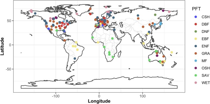
We use carbon dioxide (CO₂), water vapour (H₂O), and energy flux data from 203 sites (1,484 site years) from FLUXNET datasets^9,10. These sites cover a wide variety of climate zones and vegetation types (Extended Data Figs. 1–3, Supplementary Table 1). A previous report⁶ suggested a series of core ecosystem functional properties that can be derived from carbon, water and energy flux observations related to efficiencies or potential rates of key physiological and ecohydrological processes (for example, evapotranspiration, photosynthesis energy partitioning and so on) that control land surface–atmosphere interactions. For each site, we calculated a single set of functional properties (see ‘Calculation of ecosystem functions from FLUXNET’ in Methods for details on the calculation and definition of abbreviations): maximum gross CO₂ uptake at light saturation (GPP_sat), maximum net ecosystem productivity (NEP_max), maximum evapotranspiration (ET_max), evaporative fraction (EF) (that is, the ratio between latent heat flux and available energy, indicative of energy partitioning), EF amplitude (EF_ampl), maximum dry canopy surface conductance (G_smax), maximum and mean basal ecosystem respiration (Rb_max and Rb, respectively), and apparent carbon-use efficiency (aCUE) (that is, the remaining fraction of carbon entering the ecosystem). We also computed several metrics of growing season water-use efficiency (WUE) that account in different ways for physical evaporation and stomatal regulation effects: underlying WUE (uWUE), stomatal slope at ecosystem scale (G1), and WUE_t, a second variant of WUE, but based on transpiration estimates¹¹ (see Methods). We calculated average climate and soil water availability variables for each site, encompassing the following: cumulative soil water availability index (CSWI), mean annual precipitation (P), mean shortwave incoming radiation (SW_in), mean air temperature (T_air), and mean vapour pressure deficit during the growing season (VPD). In addition, we compiled information on canopy-scale structural variables such as foliar nitrogen concentration (N%), maximum leaf area index (LAI_max), maximum canopy height (H_c), and above-ground biomass (AGB), when available (Methods, Supplementary Table 1).

Extended Data Fig. 1. Map of the 203 FLUXNET sites used in this analysis.

Colours represent different plant functional types according to the IGBP classification. IGBP classes are: CSH (close shrublands); DBF (deciduous broadleaved forest), DNF (deciduous needleleaf forests), EBF (evergreen broadleaved forest), ENF (evergreen needleleaf forest), GRA (grasslands), MF (mixed forest), OSH (open shrublands), SAV (savannah), and WET (wetlands). The map was generated with the ggplot2 R package⁷⁴. The shape files used to create the maps were downloaded from https://github.com/ngageoint/geopackage-js.

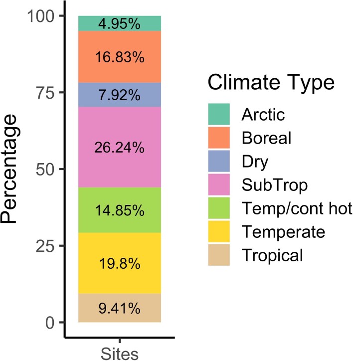
Extended Data Fig. 3. Distribution of the selected FLUXNET sites within the climate types.

Climate types were defined according to Köppen-Geiger classification as follow: Tropical (Aw, Af, Am), Dry (BSh, BSk, BWh), Temperate (Cfb), Sub-Tropical (Cfa, Csa, Csb, Cwa), Temperate/Continental Hot (Dfa, Dfb, Dwa, Dwb, Dwc), Arctic (ET)], and Boreal (Dfc, Dsc).

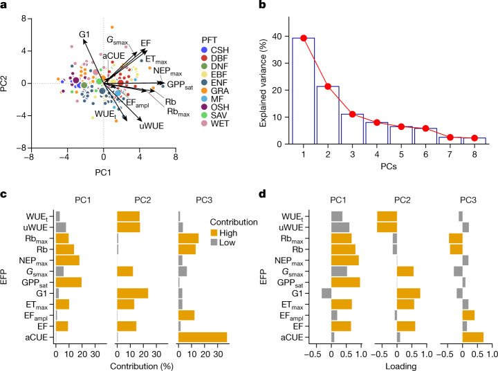
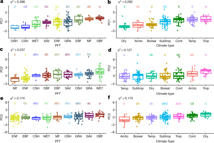
The key axes of the multi-dimensional space of terrestrial ecosystem functions were identified using principal component analysis (PCA; see Methods). We find that the first three axes of variation (the principal components; PCs) explain 71.8% of the multi-dimensional functional space variation (Fig. 1a, b, Supplementary Information 2). The first axis (PC1) explains 39.3% of the variance and is dominated by maximum ecosystem productivity properties, as indicated by the loadings of GPP_sat and NEP_max, and maximum evapotranspiration (ET_max) (Fig. 1c, d). Also, Rb contributes with positive loadings to PC1 (Fig. 1d), indicating the coupling between productivity and ecosystem respiration (both autotrophic and heterotrophic)¹². The first axis runs from sites with low productivity and evapotranspiration to sites with high photosynthesis, high net productivity, and high maximum evapotranspiration; that is, from cold and arid shrublands and wetlands, to forests in continental, tropical and temperate climates (Fig. 2a, b). The second axis (PC2) explains 21.4% of the variance and refers to water-use strategies as shown by the loadings of water-use efficiency metrics (uWUE, WUE_t, and G1), evaporative fraction and maximum surface conductance (Fig. 1c, d). Plant functional types do not explain clearly the variability of the second axis, with the exception of the evergreen and mixed forest, and the wetlands that are at the opposite extremes of the range (Fig. 2c). This axis runs (Fig. 2c,d) from temperate forests, dry and subtropical sites with a low average evaporative fraction (that is, available energy is mainly dissipated by sensible heat) but higher water-use efficiency (Fig. 2d), to sites in cold or tropical climates, as well as wetlands with a high evaporative fraction (that is, available energy is used for evapotranspiration), high surface conductance and low water-use efficiency (Fig. 2c, d). The third axis (PC3) explains 11.1% of the variance and includes key attributes that reflect the carbon-use efficiency of ecosystems. PC3 is dominated by apparent carbon-use efficiency (aCUE), basal ecosystem respiration (Rb and Rb_max) and the amplitude of EF (EF_ampl) (Fig. 1c, d). Rb and aCUE contribute to PC3 with opposite loadings, indicating that the PC3 ranges from sites with high aCUE and low Rb to sites with low aCUE and high Rb. The third axis runs from Arctic and boreal sites with low PC values to hot and dry climates (Fig. 2f), potentially indicating the imprint of aridity and temperature over the efficiency of ecosystems to use the assimilated carbon. We find no clear relation to plant functional types, with the exception of deciduous and evergreen forests that are at the extremes of the PC3 range (Fig. 2e).

Fig. 1. Key dimensions of multivariate space of terrestrial ecosystem functions.

a, Biplot resulting from the PCA. Different colours of the points represent different plant functional types (PFTs): CSH (closed shrublands); DBF (deciduous broadleaved forest); DNF (deciduous needleleaf forests); EBF (evergreen broadleaved forest); ENF (evergreen needleleaf forest); GRA (grasslands); MF (mixed forest); OSH (open shrublands); SAV (savannah); and WET (wetlands). Bigger points represent the centroid of the distribution for each PFT. b, Explained variance for each principal component. c, d, Bar plots of the contribution (c) and loading (d) of each ecosystem functional property (EFP) to each principal component. Orange bars represent the loadings and the contributions that are considered significant (Supplementary Information 2).

Fig. 2. Distribution of plant functional types and climate types along the principal components (PC1–PC3).

a, c, e, Plant functional types (PFTs). b, d, f, Climate types. Letters represent statistically significant differences in the average PCs (Tukey’s HSD test, P < 0.05), such that groups not containing the same letter are different. The effect size of the one-way ANOVA (η²) is reported (n = 203 sites). In the box plots the central line represents the mean; the lower and upper box limits correspond to the 25th and 75th percentiles and the upper (lower) whiskers extend to 1.5 (−1.5) times the interquartile range, respectively. Colours indicate different climate types and PFTs (cont, continental; subtrop, subtropical; temp, temperate; trop, tropical; PFT definitions are as in Fig. 1).

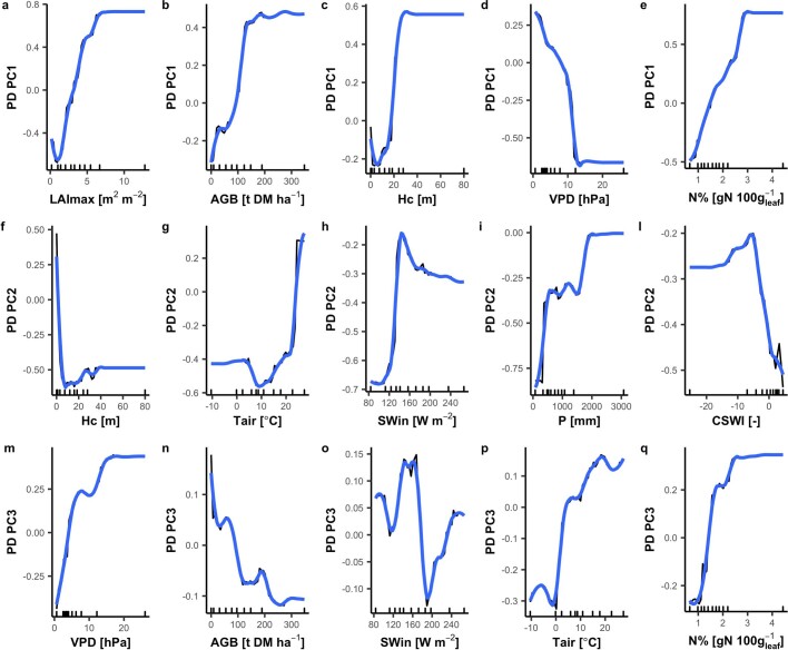
We analyse the predictive relative importance of five climatic variables (T_air, VPD, CSWI, P, and SW_in) and four vegetation structural characteristics (LAI_max, AGB, H_c and N%) on the predictability of the principal components using random forests (see ‘Predictive variable importance’ in Methods). We find that the maximum productivity axis (PC1) is largely explained by vegetation structure (LAI_max, AGB, H_c  and N%) and VPD (Fig. 3a, Extended Data Fig. 4a–e). The water-use strategies axis (PC2) is mostly explained by maximum canopy height (H_c), followed by climate variables (Fig. 3b, Extended Data Fig. 4i–l). Structural and climate variables jointly explain the variability of the carbon-use efficiency axis (PC3). The most important structural predictors of PC3 are AGB and N%, whereas VPD, T_air and SW_in are the most important climate drivers (Fig. 3c, Extended Data Fig. 4m–q).

Fig. 3. Importance of climate and vegetation properties.

a–c, Predictive relative importance for PC1 (a), PC2 (b) and PC3 (c). Numbers in the circles represent the percentage increase in mean squared error (MSE). Yellow circles represent vegetation structural variables; light blue circles represent climate variables.

Extended Data Fig. 4. Results of the relative importance analysis conducted with the Random Forest and partial dependence.

See ‘Predictive variable importance’ in Methods. The slopes of the partial dependence plot indicate the sensitivity of the response (PCs) to the specific predictor. The out-of-bag cross-validation leads to predictive explained variance of 56.76% for PC1, 30.24% for PC2, and 20.41% for PC3. The portion of unexplained variance might be related to missing leaf traits predictor such as leaf mass per area or phenological traits. The partial dependence plots of all variables are shown: top panels for PC1 (a–e), middle panels for PC2 (f–l), and bottom panels for PC3 (m–q). The blue lines represent the locally estimated scatterplot (LOESS) smoothing of the partial dependence. Tick marks in the x axis represent the minimum, maximum and deciles of the variable distribution.

The dependencies described above can only be interpreted causally if the regression models are in fact causal regression models (see Supplementary Information 3 for a formal definition). In many situations, this fails to be the case owing to the existence of hidden confounders; that is, unmeasured variables that influence both the principal components and the covariates (here climate and structural variables)¹³. Using an invariance-based analysis (see ‘Invariant causal regression models and causal variable importance’ in Methods), we find evidence that the full regression model including all the selected structural and climatic variables might be causal (Supplementary Information 3.2.1, Supplementary Fig. 3.3). If this is indeed the case, we can make the following statements. When considering groupwise causal variable importance, we can conclude that vegetation structure is a stronger causal driver than climate of the spatial (that is, across sites) variability of the maximum realized productivity axis (PC1) (Supplementary Fig. 3.7), and both are significant (Supplementary Table 3.2). Consider two contiguous plots of forest experiencing the same climate conditions, one disturbed and the other not. The undisturbed forest, which is likely to be taller, with higher LAI and carbon stocks, would probably have higher maximum photosynthetic rates and net ecosystem production, which are the most important variables loading on the first axis. Although, in time, the variability of climate controls the variability of gross and net CO₂ uptake and productivity^14,15, which are variables related to the maximum productivity axis (PC1), in space (that is, across sites) we find only a marginal control in very cold and radiation-limited sites (Extended Data Fig. 5a for a PC1 map), or for very warm and high atmospheric aridity (high VPD) conditions (Extended Data Fig. 4d based on predictive variable importance). Both vegetation structure and climate variables seem to have a joint direct causal effect on PC2 (Supplementary Fig 3.7). Although vegetation canopy height is constrained by resource availability¹⁶, particularly water, our results suggest that it acts itself as a control on the water-use strategies axis (PC2) and that it has a stronger causal effect on PC2 than each of the climate variables (Supplementary Fig. 3.6). The importance of vegetation height for ecosystem water-use strategies is manifold. First, vegetation height controls the coupling between stomata and atmosphere by influencing surface roughness and then aerodynamic resistance¹⁷, which modulates leaf-to-air VPD and water use efficiency. Second, vegetation height reflects variation in water-use efficiency that decreases as a consequence of progressive hydraulic constraints on stomatal conductance to water vapour and growth in taller vegetation¹⁶. Third, canopy height might reflect stand age and it is influenced by disturbances. Studies on forest chronosequence show a more conservative use of water in younger forests, which results in higher water-use efficiency¹⁸. We cannot exclude that our results are indirectly affected by the gradient from grass to forests, but postulate that these effects are likely to be minimal (Extended Data Fig. 6). Vegetation structure has a direct causal effect on the carbon-use efficiency axis (PC3; Supplementary Fig 3.7). Previous studies show that vegetation structure reflects climatic constraints but also the successional stage of an ecosystem after disturbance¹⁹. Increasing stand age—which is typically associated with higher above-ground biomass—is also associated with reduced forest production efficiency²⁰. The negative partial dependence of PC3 on above-ground biomass (Extended Data Fig. 4n, based on predictive variable importance) is likely to be related to higher autotrophic and heterotrophic respiration rates per unit of CO₂ taken up by photosynthesis as biomass increases²¹. The positive dependence of PC3 on N% (Extended Data Fig. 4q, based on predictive variable importance) supports previous findings that carbon-use efficiency might be controlled by the nutrient status of the vegetation²².

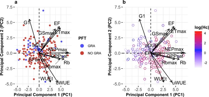
Extended Data Fig. 6. Biplot resulting from the principal component analysis.

Plot as in Fig. 1. In panel a, points are colour-coded by grass vs. non-grass classes. In panel b, the points are colour-coded according to the logarithm of vegetation height. From these results we conclude that there is not a clear cluster in the biplot for grass and non-grass vegetation. In fact, in Extended Data Fig. 6a, the sites do not cluster according to the designation to grasslands or not, but there is a clear gradient as a function of the vegetation height (Extended Data Fig. 6b).

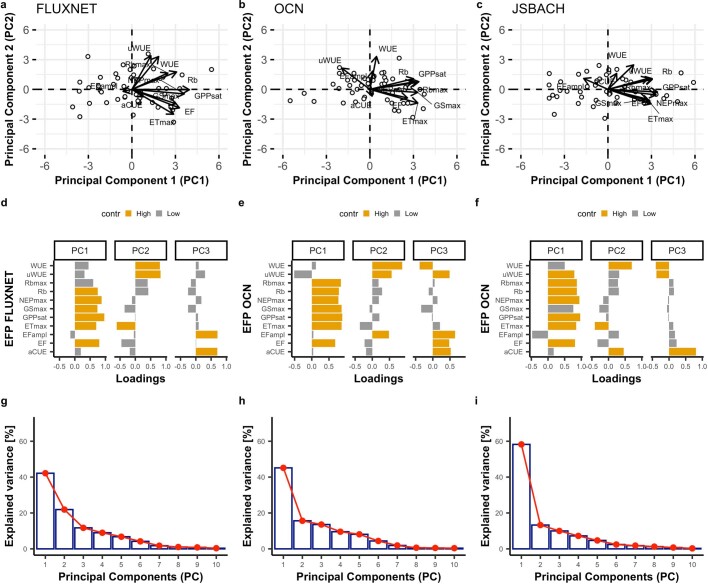
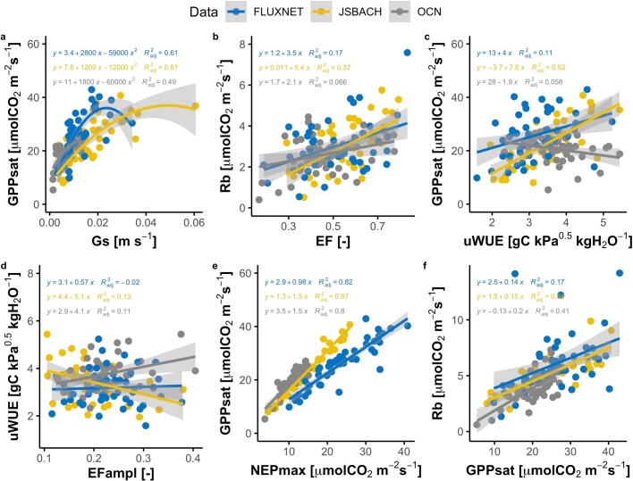
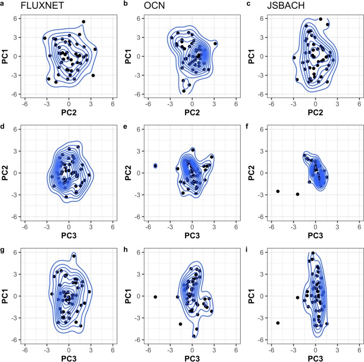
The two representative—yet complementary—land surface models examined here (OCN and JSBACH) partially reproduce the main axes of terrestrial ecosystem functions (Extended Data Fig. 7). This is shown when comparing the PCA calculated from FLUXNET data with simulated ecosystem functional properties from 48 site-level runs, mostly in temperate and boreal sites (Extended Data Fig. 7). The models are broadly consistent with the FLUXNET observations in the description of the potential productivity axis (PC1), but diverge in the description of the water-use strategies (PC2) and the carbon-use efficiency (PC3) axes. Despite the overall good agreement between observed and modelled fluxes at a half-hourly timescale (Supplementary Table 4), we show that, first, models are limited in simulating the relationships between ecosystem functions (Extended Data Fig. 8); and, second, models tend to overstate observed correlation strengths among ecosystem functions, as shown by the larger variance explained by the PC1 in models compared to observations (Extended Data Fig 7h, i). As a result, the ecosystem functional space that can be simulated by the models, represented by the area shown in Extended Data Fig. 9, is smaller than that expected from observations, particularly in the plane spanned by the PC2 and PC3 (Extended Data Fig. 9d–f). The limited variability of the model output points to an insufficient representation of the actual variability of the vegetation properties by the average parameterization of plant functional types. Uncertain implementation of plant hydraulics and water acquisition or conservation strategies in land surface models is a key limitation²³ that explains the observed discrepancy in PC2. With regard to PC3, one limitation is that models lack flexibility in representing the response of respiration rates and carbon-use efficiency to climate, nutrients, disturbances and substrate availability (including biomass and stand age)^20,24.

Extended Data Fig. 7. Comparing observed and modelled global ecosystem functional trade-offs.

PCA for a subset of 48 FLUXNET sites mainly distributed in temperate and boreal regions and 2 different land surface models (Supplementary Table 1). The left column is FLUXNET, the centre column is OCN, and the right column is JSBACH. Panels a, b, c: the biplot resulting from the PCA. Panels d, e, f, bar plot of the loading of each ecosystem functional property to each principal component. Orange bars represent the loadings that are selected as significant and with high contribution (Supplementary Information 2). Panels g, h, i report the variance explained by each principal component. EFP acronym list: apparent carbon-use efficiency (aCUE), evaporative fraction (EF), amplitude of EF (EF_ampl), maximum evapotranspiration (ET_max), gross primary productivity at light saturation (GPP_sat), maximum surface conductance (G_smax), maximum net ecosystem productivity (NEP_max), maximum and mean basal ecosystem respiration (Rb_max and Rb, respectively), and growing season underlying water-use efficiency (uWUE). Note that the PCA results for FLUXNET (panels a, d, g) are different from Fig. 1 because here we use the subset of 48 sites used for the modelling analysis.

Extended Data Fig. 8. Pairwise relationship between some key ecosystem functional properties derived from FLUXNET, and modelled with JSBACH and OCN.

n = 48 sites; see Supplementary Table 1. The grey areas represent the 95% confidence interval of the linear and nonlinear regression. Overall the correlation between modelled functions is larger than in the observations. Acronym list: evaporative fraction (EF), amplitude of EF (EF_ampl), gross primary productivity at light saturation (GPP_sat), maximum surface conductance (G_s), maximum net ecosystem productivity (NEP_max), basal ecosystem respiration (Rb), and growing season underlying water-use efficiency (uWUE).

Extended Data Fig. 9. Representation of the 2D ecosystem functional properties space derived from FLUXNET observations and land surface model runs (OCN, JSBACH).

The points represent the principal component (PC) value calculate for each site. The contour lines are computed using a 2D kernel density estimates. The contour lines show the area occupied by ecosystem functional properties and its boundary that, according to the results of the analysis, are set by vegetation characteristics (PC1), water availability, abiotic limitations, and vegetation height (PC2), and above-ground biomass, foliar nitrogen and atmospheric aridity (PC3). The areas computed for FLUXNET are wider than for the models, particularly for PC2 and PC3. This means that ecosystem functional properties as simulated by models are more constrained than for the observations.

The identification of the key axes of terrestrial ecosystem function and their relationships with climate and vegetation structure will help to support the development of the next generation of land surface models and complement their benchmarking²⁵. By comparing the contributions of the functions and their loadings to the principal components, we can assess whether the representations of ecosystem functions in the models and in the ‘real world’ are coherent, and if not, which key processes or model formulations need improvement. For example, we show that vegetation height controls the water-use strategies axis (PC2), which is not well reproduced by the land surface models²³. This suggests that future land surface models need to include a representation of water-use strategies that explicitly accounts for hydraulic limitations to growth, vegetation stature, vertical and horizontal structures and microenvironments of the canopy, and a refined parameterization of stomatal control. Likewise, the inclusion of a flexible representation of carbon-use efficiency would enable models to reproduce the third axis of ecosystem functions²⁴. The comparison of the variances explained by functional axes and the loadings of the functions in simulated and observed data will indicate whether simulated ecosystem functions are appropriately coordinated. The overly tight coupling of ecosystem functions by models indicates a lack of flexibility in ecosystem responses to environmental drivers, such as adaptive carbon and water couplings.

In summary, by analysing a consistent set of ecosystem functions across major terrestrial biomes and climate zones, we show that three key axes capture the terrestrial ecosystem functions. The first and most important axis represents maximum productivity and is driven primarily by vegetation structure, followed by mean climate. The second axis is related to water-use strategies, and is driven by vegetation height. The third axis is related to ecosystem carbon-use efficiency; it is controlled by vegetation structure, but shows a gradient related to aridity. We find that the plant functional type concept does not necessarily capture the variability of ecosystem functions, because the majority of plant functional types are evenly distributed along the water-use strategies (PC2) and carbon-use efficiency (PC3) axes. Our approach allows the overall functioning of terrestrial ecosystems to be summarized and offers a way towards the development of metrics of ecosystem multifunctionality⁵—a measure of ecosystem functions as a whole, which is crucial to achieving a comprehensive assessment of the responses of ecosystems to climate and environmental variability, as well as biodiversity losses⁵. The analysis focuses on relatively few critical functions related to carbon, water and energy cycling of ecosystems. To attain a fully comprehensive characterization of the key axes of terrestrial ecosystem functions, more parameters related to nutrient cycling, seed dispersal and chemical defences—among others—should be included. The concept of the key axes of ecosystem functions could be used as a backdrop for the development of land surface models, which might help to improve the predictability of the terrestrial carbon and water cycle in response to future changing climatic and environmental conditions.

Methods

FLUXNET data

The data used in this study belong to the FLUXNET LaThuile⁹ and FLUXNET2015 Tier 1 and Tier 2 datasets¹⁰, which make up the global network of CO₂, water vapour and energy flux measurements. We merged the two FLUXNET releases and retained the FLUXNET2015 (the most recent and with a robust quality check) version of the data when the site was present in both datasets. Croplands were removed to avoid the inclusion of sites that are heavily managed in the analysis (for example, fertilization and irrigation).

The sites used cover a wide variety of climate zones (from tropical to Mediterranean to Arctic) and vegetation types (wetlands, shrublands, grasslands, savanna, evergreen and deciduous forests). It should be noted though that tropical forests are underrepresented in the FLUXNET database (Extended Data Figs. 1, 3).

Sites were excluded in cases in which: (i) data on precipitation or radiation were not available or completely gap-filled; (ii) the calculation of functional properties failed because of low availability of measured data (see ‘Calculation of ecosystem functions from FLUXNET’); and (iii) fluxes showed clear discontinuities in time series indicating a change of instrumentation set-up (for example, changes in the height of the ultrasonic anemometer or gas analyser).

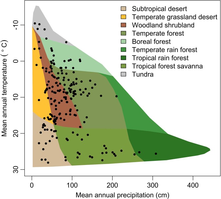
The final number of sites selected was 203 (1,484 site years). The geographical distribution is shown in Extended Data Fig. 1, the distribution in the climate space is shown in Extended Data Fig. 2 and the fraction of sites for each climate classes is reported in Extended Data Fig. 3.

Extended Data Fig. 2. FLUXNET sites used in the analysis plotted in the precipitation–temperature space.

The background represent climate space of the major biomes according to Whittaker⁷⁵ and further modifications⁷⁶. Biomes are defined as function of the mean annual temperature and mean annual precipitation (MAP). The figure is modified from Liu et al.,⁷⁷ using the code available in git (https://github.com/kunstler/BIOMEplot).

For each site, we downloaded the following variables at half-hourly temporal resolution: (i) gross primary productivity (GPP, μmol CO₂ m^–2 s^–1) derived from the night-time flux partitioning²⁶ (GPP_NT_VUT_50 in FLUXNET 2015 and GPP_f in LaThuile), (ii) net ecosystem exchange (NEE, μmol CO₂ m^–2 s^–1) measurements filtered using annual friction velocity (u*, m s⁻¹) threshold (NEE_VUT_50 in FLUXNET 2015; NEE in LaThuile); (iii) latent heat (LE, W m⁻²) fluxes, which were converted to evapotranspiration (ET, mm); (iv) sensible heat (H, W m⁻²) fluxes; (v) air temperature (T_air, °C); (vi) vapour pressure deficit (VPD, hPa); (vii) global shortwave incoming radiation (SW_in, W m⁻²); viii) net radiation (R_n, W m⁻²); (ix) ground heat flux (G, W m⁻²); (x) friction velocity u* (m s⁻¹); and (xi) wind speed (u, m s⁻¹). For the energy fluxes (H, LE) we selected the fluxes not corrected for the energy balance closure to guarantee consistency between the two FLUXNET datasets (in the LaThuile dataset energy fluxes were not corrected).

The cumulative soil water index (CSWI, mm) was computed as a measure of water availability according to a previous report²⁷. Half-hourly values of transpiration estimates (T, mm) were calculated with the transpiration estimation algorithm (TEA)²⁸. The TEA has been shown to perform well against both model simulations and independent sap flow data²⁸.

For 101 sites, ecosystem scale foliar N content (N%, gN 100 g⁻¹) was computed as the community weighted average of foliar N% of the major species at the site sampled at the peak of the growing season or gathered from the literature^29–32. Foliar N% for additional sites was derived from the FLUXNET Biological Ancillary Data Management (BADM) product and/or provided by site principal investigators (Supplementary Table 1, Extended Data Fig. 1). It should be noted that this compilation of N% data might suffer from uncertainties resulting from the scaling from leaves to the eddy covariance footprint, the sampling strategy (including the position along the vertical canopy profile), the species selection and the timing of sampling. About 30% of the data comes from a coordinated effort that minimized these uncertainties^29,30, and for the others we collected N% data that were representative for the eddy covariance footprint^31,32.

Maximum leaf area index (LAI_max, m² m⁻²) and maximum canopy height (H_c, m) were also collected for 153 and 199 sites, respectively, from the literature^32,33, the BADM product, and/or site principal investigators.

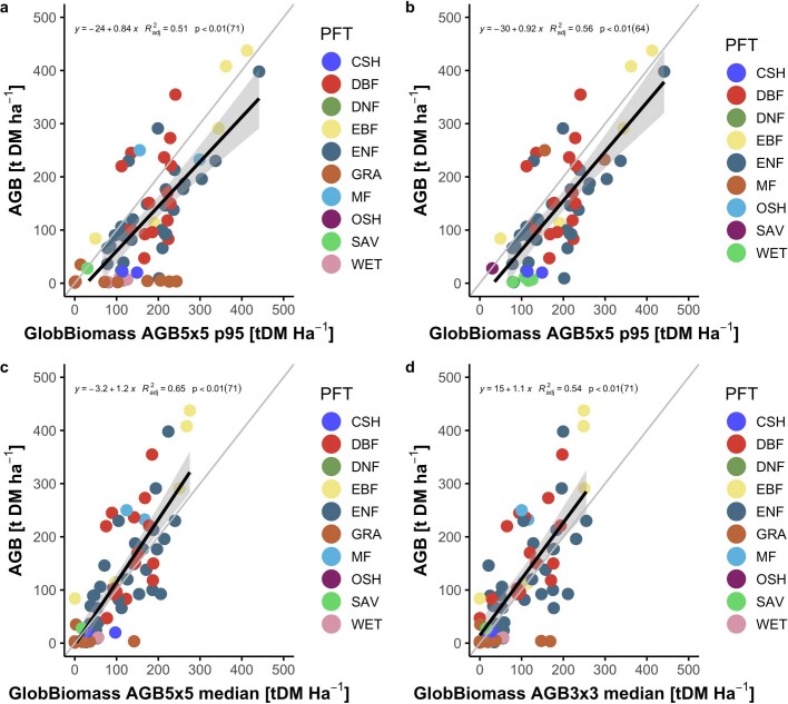
Earth observation retrievals of above-ground biomass (AGB, tons of dry matter per hectare (t DM ha⁻¹)) were extracted from the GlobBiomass dataset³⁴ at its original resolution (grid cell 100 × 100 m) for each site location. All the grid cells in a 300 × 300 m and 500 × 500 m window around each location were selected to estimate the median and 95th percentiles of AGB for each site. The median of AGB was selected to avoid the contribution of potential outliers to the expected value of AGB. The analysis further explored the contribution of higher percentiles in the local variation of AGB as previous studies have highlighted the contribution of older and larger trees in uneven stand age plots to ecosystem functioning³⁵. According to the evaluation against AGB measured at 71 FLUXNET sites (Extended Data Fig. 10), we decided to use the product with median AGB values extracted from the 500 × 500 m window.

Extended Data Fig. 10. Evaluation of above-ground biomass satellite products against FLUXNET observation.

n = 71. We evaluated the three above-ground biomass (AGB, t DM ha⁻¹) products derived from the GlobBiomass dataset as reported in the Method section. From the product at its original resolution (100 x 100 m) we extracted the 95th percentile of the estimated AGB in 5 by 5 grid cell windows (AGB5x5, panel a with all sites, and panel b with the grasslands excluded) centered around the location of the FLUXNET sites used for the evaluation. Further, we extracted the median in 3 by 3 and 5 by 5 grid cells centered around the location of the FLUXNET site (panels c and d). Total above-ground biomass observations were gathered from the BADM dataset downloaded from the AMERIFLUX network and from the FLUXNET LaThuile release. Only data with the clear indication of the unit of AGB expressed in in dry matter (t DM ha⁻¹) were retained for the analysis. Results show that the median of the 5 by 5 grid cell window (panel c) is the best extraction method to characterize AGB at the FLUXNET sites, and therefore retained for further analysis. Adjusted determination coefficient (R²), linear regression function, and p-value calculated with the F-test are also reported.

A total of 94 sites have all the data on vegetation structure (N%, LAI_max, H_c, and AGB).

The list of sites is reported in Supplementary Table 1 along with the plant functional type (PFT), Köppen-Geiger classification, coordinates, and when available N%, LAI_max, H_c and AGB.

In this study we did not make use of satellite information, with the exception of the AGB data product. Future studies will benefit from new missions such as the ECOsystem Spaceborne Thermal Radiometer Experiment on Space Station (ECOSTRESS), the fluorescence explorer (FLEX), hyperspectral, and radar and laser detection and ranging (LiDAR) missions (for example, Global Ecosystem Dynamics Investigation (GEDI)), to characterize a multivariate space of structural and functional properties.

Calculation of ecosystem functions from FLUXNET

Starting from half-hourly data, we calculated at each site a single value for each of the ecosystem functions listed below. For the calculations of functional properties we used, unless otherwise indicated, good-quality data: quality flag 0 (measured data) and 1 (good-quality gap-filled data) in the FLUXNET dataset.

Gross primary productivity at light saturation (GPP_sat)

GPP at light saturation using photosynthetically active radiation as driving radiation and 2,000 μmol m⁻² s⁻¹ as saturating light. GPP_sat represents the ecosystem-scale maximum photosynthetic CO₂ uptake^15,30,36. The GPP_sat was estimated from half-hourly data by fitting the hyperbolic light response curves with a moving window of 5 days and assigned at the centre of the moving window^30,37. For each site the 90th percentile from the GPP_sat estimates was then extracted.

Maximum net ecosystem productivity (NEP_max)

This was computed as the 90th percentile of the half-hourly net ecosystem production (NEP = −NEE) in the growing season (that is, when daily GPP is higher than 30% of the GPP amplitude). This metric represents the maximum net CO₂ uptake of the ecosystem.

Basal ecosystem respiration (Rb and Rb_max)

Basal ecosystem respiration at reference temperature of 15 °C was derived from night-time NEE measurements²⁶. Daily basal ecosystem respiration (Rb_d) was derived by fitting an Arrhenius type equation over a five-day moving window and by keeping the sensitivity to temperature parameter (E₀) fixed as in the night-time partitioning algorithms^26,38. Rb_d varies across seasons because it is affected by short-term variations in productivity^33,39, phenology⁴⁰ and water stress⁴¹. For each site, the mean of the Rb_d (Rb) and the 95^th percentile (Rb_max) were computed. The calculations were conducted with the REddyProc R package v.1.2.2 (ref. ³⁸).

Apparent carbon-use efficiency (aCUE)

The aCUE as defined in this study is the efficiency of an ecosystem to sequester the carbon assimilated with photosynthesis³⁹. aCUE is an indication of the proportion of respired carbon with respect to assimilated carbon within one season. A previous report⁶ showed that little of the variability in aCUE can be explained by climate or conventional site characteristics, and suggested an underlying control by plant, faunal and microbial traits, in addition to site disturbance history. Daily aCUE (aCUE_d) is defined as aCUE_d = 1 − (Rb_d/GPP_d), where GPP_d is daily mean GPP and Rb_d is derived as described above. For each site, aCUE was computed as the median of aCUE_d.

Metrics of water-use efficiency (WUE)

Various metrics of WUE are described below: stomatal slope or slope coefficient (G1), underlying water-use efficiency (uWUE), and water-use efficiency based on transpiration (WUE_t). The three metrics were used because they are complementary, as shown in previous studies^11,42.

Stomatal slope or slope coefficient (G1)

This is the marginal carbon cost of water to the plant carbon uptake. G1 is the key parameter of the optimal stomatal model derived previously⁴³. G1 is inversely related to leaf-level WUE. At leaf level, G1 is calculated using nonlinear regression and can be interpreted as the slope between stomatal conductance and net CO₂ assimilation, normalized for VPD and CO₂ concentration⁴³. A previous report⁴² showed the potential of the use of G1 at ecosystem scale, where stomatal conductance is replaced by surface conductance (G_s), and net assimilation by GPP. The methodology is implemented in the bigleaf R package⁴⁴. The metric was computed in the following situations: (i) incoming shortwave radiation (SW_in) greater than 200 W m⁻²; (ii) no precipitation event for the last 24 h⁴⁵, when precipitation data are available; and (iii) during the growing season: daily GPP > 30% of its seasonal amplitude⁴⁴.

Underlying water-use efficiency (uWUE)

The underlying WUE was computed following a previous method⁴⁶. uWUE is a metric of water-use efficiency that is negatively correlated to G1 at canopy scale⁴⁴:

$$\mathrm{uWUE}=\frac{\mathrm{GPP}\sqrt{\mathrm{VPD}}}{\mathrm{ET}}.$$

uWUE was calculated using the same filtering that was applied for the calculation of G1. The median of the half-hourly retained uWUE values was computed for each site and used as a functional property.

Water-use efficiency based on transpiration (WUE_t)

The WUE based on transpiration (T) was computed to reduce the confounding effect resulting from soil evaporation^11,28:

$${\mathrm{WUE}}_{\mathrm{t}}=\frac{\mathrm{GPP}}{T},$$

where T is the mean annual transpiration calculated with the transpiration estimation algorithm (TEA) developed by in a previous study²⁸ and GPP is the mean annual GPP.

Maximum surface conductance (G_smax)

Surface conductance (G_s) was computed by inverting the Penman–Monteith equation after calculating the aerodynamic conductance (G_a).

Among the different formulations of G_a (m s^–1) in the literature, we chose to use here the calculation of the canopy (quasi-laminar) boundary layer conductance to heat transfer, which ranges from empirical to physically based (for example, ref. ⁴⁷). Other studies^48,49 suggested an empirical relationship between G_a, the horizontal wind speed (u) and the friction velocity, u*:

$$G_{\mathrm{a}}=\frac{1}{\left(\frac{u}{u^{*2}}+6.2u{*}^{-0.67}\right)}$$

G_s (m s⁻¹) is computed by inverting the Penman–Monteith equation:

$$G_{\mathrm{s}}=\frac{{\mathrm{LEG}}_{\mathrm{a}}\gamma }{\mathrm{\Delta }\left(R_{\mathrm{n}}-G-S\right)+\rho C_{\mathrm{p}}{G}_{\mathrm{a}}\mathrm{VPD}-\mathrm{LE}\left(\mathrm{\Delta }+\gamma \right)}$$

where Δ is the slope of the saturation vapour pressure curve (kPa K⁻¹), ρ is the air density (kg m⁻³), C_p is the specific heat of the air (J K⁻¹ kg⁻¹), γ is the psychrometric constant (kPa K⁻¹), VPD (kPa), R_n (W m⁻²), G (W m⁻²) and S is the sum of all energy storage fluxes (W m⁻²) and set to 0 as not available in the dataset. When not available, G also was set to 0.

G_s represents the combined conductance of the vegetation and the soil to water vapour transfer. To retain the values with a clear physiological interpretation, we filtered the data as we did for the calculation of G1.

For each site, the 90th percentile of the half-hourly G_s was calculated and retained as the maximum surface conductance of each site (G_smax). G_s was computed using the bigleaf R package⁴⁴.

Maximum evapotranspiration in the growing season (ET_max)

This metric represents the maximum evapotranspiration computed as the 95th percentile of ET in the growing season and using the data retained after the same filtering applied for the G1 calculation.

Evaporative fraction (EF)

EF is the ratio between LE and the available energy, here calculated as the sum of H + LE (ref. ⁵⁰). For the calculation of EF, we used the same filtering strategy as for G1. We first calculated mean daytime EF. We then computed  the EF per site as the growing season average of daytime EF. We also computed the amplitude of the EF in the growing season by calculating the interquartile distance of the distribution of mean daytime EF (EF_ampl).

Principal component analysis

A PCA was conducted on the multivariate space of the ecosystem functions. Each variable (ecosystem functional property, EFP) was standardized using z-transformation (that is, by subtracting its mean value and then dividing by its standard deviation). From the PCA results we extracted the explained variance of each component and the loadings of the EFPs, indicating the contribution of each variable to the component. We performed the PCA using the function PCA() implemented in the R package FactoMineR⁵¹.

We justify using PCA over nonlinear methods because it is an exploratory technique that is highly suited to the analysis of the data volume used in this study, whereas other nonlinear methods applied to such data would be over-parameterized. For the same reason, PCA was used in previous work concerning the global spectrum of leaf and plant traits, and fluxes^1,3,52.

To test the significance of dimensionality of the PCA, we used a previously described methodology⁵³. We used the R package ade4 (ref. ⁵⁴) and evaluated the number of significant components of the PCA to be retained to minimize both redundancy and loss of information (Supplementary Information 2). We tested the significance of the PCA loadings using a combination of the bootstrapped eigenvector method⁵⁵ and a threshold selected using the number of dimensions⁵⁶ (Supplementary Information 2).

Predictive variable importance

A random forests (RF) analysis was used to identify the vegetation structure and climate variables that contribute the most to the variability of the significant principal components, which were identified with the PCA analysis (see ‘Principal component analysis’). In the main text we refer to the results of this analysis as ‘predictive variable importance’ to distinguish this to the ‘causal variable importance’ described below.

The analysis was conducted using the following predictor variables: as structural variables, N% (gN 100 g⁻¹), LAI_max (m₂ m⁻²), AGB (t DM ha⁻¹) and H_c (m); as climatic variables, mean annual precipitation (P, mm), mean VPD during the growing season (VPD, hPa), mean shortwave radiation (SW_in, W m⁻²), mean air temperature (T_air, °C); and the cumulative soil water index (CSWI, −), as indicator of site water availability.

We used partial dependencies of variables to assess the relationship between individual predictors and the response variable (that is, PC1, PC2 and PC3).

The results from the partial dependency analysis can be used to determine the effects of individual variables on the response, without the influence of the other variables. The partial dependence function was calculated using the pdp R package⁵⁷.

The partial dependencies were calculated restricted to the values that lie within the convex hull of their training values to reduce the risk of interpreting the partial dependence plot outside the range of the data (extrapolation).

Invariant causal regression models and causal variable importance

We have quantified the dependence of the principal components on the different structural and climatic variables using nonlinear regression. Such dependencies can only be interpreted causally if the regression models are in fact causal regression models (see Supplementary Information 3 for a formal definition), which may not be the case if there are hidden confounders. To see whether the regression models allow for a causal interpretation, we use invariant causal prediction⁵⁸. This method investigates whether the regression models are stable with respect to different patterns of heterogeneity in the data, encoded by different environments (that is, subsets of the original dataset). The rationale is that a causal model, describing the full causal mechanism for the response variable, should be invariant with respect to changes in the environment if the latter does not directly influence the response variable^13,59. Other non-causal models may be invariant, too, but a non-invariant model cannot be considered causal.

How to choose the environments is a modelling choice that must satisfy the following criteria. First, it should be possible to assign each data point to exactly one environment. Second, the environments should induce heterogeneity in the data, so that, for example, the predictor variables have different distributions across environments. Third, the environments must not directly affect the response variable, only via predictors, although the distribution of the response may still change between environments. The third criterion can be verified by expert knowledge and is assumed to hold for our analysis. In addition, if it is violated, then, usually, no set is invariant⁵⁸, which can be detected from data.

In our analysis, we assigned each data point (that is, each site) to one of two environments (two subsets of the original dataset): the first includes forest sites in North America, Europe or Asia; and the second includes non-forest and forest ecosystems from South America, Africa or Oceania, and non-forest ecosystems from North America, Europe or Asia (see Supplementary Information 3.1.3.1 for details). Our choice satisfies the method’s assumption that the distribution of the predictors is different between the two environments (that is, they induce heterogeneity in the data; see Supplementary Fig. 3.1). Environments that are too small or too homogeneous do not provide any evidence against the full set of covariates being a candidate for the set of causal predictors. Other choices of environments than the one presented here yield consistent results (Supplementary Information 3.2.1, Supplementary Fig. 3.4).

For each subset of predictors, we test whether the corresponding regression model is invariant (yielding the same model fit in each environment). Although many models were rejected and considered non-invariant, the full model (with all the nine predictors and used in the predictive variable importance analysis) was accepted as invariant, establishing the full set of covariates as a reasonable candidate for the set of direct causal predictors. We used both RF (randomForest package in R⁶⁰) and generalized additive models, GAM⁶¹ (mgcv package⁶² in R) to fit the models. Both methods lead to comparable results but with a better average performance of the RF: GAM led to slightly better results than RF for PC1, whereas for PC2 and PC3 RF showed a much better model performance (Supplementary Table 3.1, Supplementary Information 3.2.2). Therefore, in the main text we showed only the results from the RF (except for PC1).

If, indeed, the considered regression models are causal, this allows us to make several statements. First, we can test for the existence of causal effects by testing for statistical significance of the respective predictors in the fitted models. Second, we can use the response curves of the fitted model to define a variable importance measure with a causal interpretation. In the main text we refer to this variable importance as ‘causal variable importance’. For details, see Supplementary Information 3.1.2. More formally, we considered the expected value of the predicted variables (the principal components) under joint interventions on all covariates (AGB, H_c, LAI_max, N%, T_air, VPD, SW_in, CSWI and P) at once, and then, to define the importance, we quantified how this expected value depends on the different covariates. We applied the same analysis to groups of vegetation structural and climate covariates (see ‘Groupwise variable importance’ in Supplementary Information 3.1.2.3, 3.2.3).

The details of the methodology and the results are described in Supplementary Information 3, in which we also provide further details on the choice of environment variable and on the statistical tests that we use to test for invariance. An overview of the invariance-based methodology is shown in Supplementary Fig. 3.1.

Land surface model runs

We run two widely used land surface models: Orchidee-CN (OCN) and Jena Scheme for Biosphere Atmosphere Coupling in Hamburg (JSBACH):

OCN

The dynamic global vegetation model OCN is a model of the coupled terrestrial carbon and nitrogen cycles^63,64, derived from the ORCHIDEE land surface model. It operates at a half-hourly timescale and simulates diurnal net carbon, heat and water exchanges, as well as nitrogen trace gas emissions, which jointly affect the daily changes in leaf area index, foliar nitrogen, and vegetation structure and growth. The main purpose of the model is to analyse the longer-term (interannual to decadal) implication of nutrient cycling for the modelling of land–climate interactions^64,65. The model can run offline, driven by observed meteorological parameters, or coupled to the global circulation model.

JSBACH

JSBACH v.3 is the land surface model of the MPI Earth System Model^66,67. The model operates at a half-hourly time step and simulates the diurnal net exchange of momentum, heat, water and carbon with the atmosphere. Daily changes in leaf area index and leaf photosynthetic capacity are derived from a prognostic scheme assuming a PFT-specific set maximum leaf area index and a set of climate responses modulating the seasonal course of leaf area index. Carbon pools are prognostic allowing for simulating the seasonal course of net land–atmosphere carbon exchanges.

We selected OCN and JSBACH because they are widely used land surface models with different structures. JSBACH is a parsimonious representation of the terrestrial energy, water and carbon exchanges used to study the coupling of land and atmosphere processes in an Earth system model⁶⁷. OCN has also been derived from the land surface model ORCHIDEE⁶⁸, but it includes a more comprehensive representation of plant physiology, including a detailed representation of the tight coupling of the C and N cycling⁶³. Both models contribute to the annual global carbon budget of the Global Carbon Project⁶⁹ and have shown good performance compared to a number of global benchmarks. OCN was further used in several model syntheses focused on the interaction between changing N deposition and CO₂ fertilization^70–72. Both OCN and JSBACH can operate at a half-hourly timescale and simulate net and gross carbon exchanges, water and energy fluxes, and therefore are ideal for the extraction of ecosystem functional properties, as done with the eddy covariance data.

The models were driven by half-hourly meteorological variables (shortwave and longwave downward flux, air temperature and humidity, precipitation, wind speed and atmospheric CO₂ concentrations) observed at the eddy covariance sites. OCN was furthermore driven by N deposition fields⁷³. Vegetation type, soil texture and plant available water were prescribed on the basis of site observations, but no additional site-specific parameterization was used. Both models were brought into equilibrium with respect to their ecosystem water storage and biogeochemical pools by repeatedly looping over the available site years. We added random noise (mean equal to 0 and standard deviation of 5% of the flux value) to the fluxes simulated by the models to mimic the random noise of the eddy covariance flux observations. An additional test conducted without noise addition showed only a marginal effect on the calculations of the functional properties and the ecosystem functional space.

We used runs of the JSBACH and OCN model for 48 FLUXNET sites (Supplementary Table 1). The simulated fluxes were evaluated against the observation to assess the performance of the models at the selected sites. From the model outputs and from each site we derived the ecosystem functions using the same methodology described above. Then the PCA analysis was performed on the three datasets (FLUXNET, OCN and JSBACH) and restricted to the 48 sites used to run the models. We ran the models only on the subset of sites for which the information for the parameterization and high-quality forcing was available. However, the different ecosystem functions emerge from the model structure and climatological conditions. Therefore, even with a smaller set of site we can evaluate whether models reproduce the key dimensions of terrestrial ecosystem function by comparing the PCA results from FLUXNET and the model runs.

Reporting summary

Further information on research design is available in the Nature Research Reporting Summary linked to this paper.

Online content

Any methods, additional references, Nature Research reporting summaries, source data, extended data, supplementary information, acknowledgements, peer review information; details of author contributions and competing interests; and statements of data and code availability are available at 10.1038/s41586-021-03939-9.

Extended data figures and tables

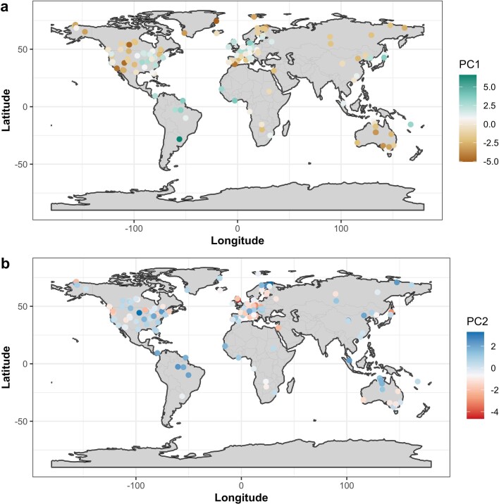
Extended Data Fig. 5. Map of FLUXNET sites colour-coded for the value of PC1 and PC2.

a, PC1. b, PC2. The map of the PC1 shows the areas of the globe with high productivity (positive values of PC1 in the temperate areas, Eastern North America, Eastern Asia, and Tropics), and areas characterized by lower productivity (Semi-arid regions, high latitude and Mediterranean ecosystems). The map of the PC2 shows the gradient of evaporative fraction and the spatial patterns of water use efficiency. This PC2 runs from sites with a high evaporative fraction (i.e. available energy is dissipated preferentially to evaporated or transpired water), high surface conductance, and low water use efficiency (positive PC2 values), to water limited sites (i.e. low evaporative fraction where available energy is mainly dissipated by sensible heat) that also show higher water-use efficiency (negative PC2 values). The maps were generated with the ggplot2 R package⁷⁴. The shape files used to create the maps were downloaded from https://github.com/ngageoint/geopackage-js.

Author contributions

M.M., M. Reichstein, M.D.M. and T.M. conceived the study. M.M. and T.M. performed the majority of the analysis. R.C. and J. Peters designed and coded the causality analysis. J.A.N. provided the transpiration partitioning data. J. Knauer and S.Z. performed the land surface model runs. N.C. and U.W. processed the above-ground biomass data. O.P.-P. provided support with data analysis and discussions. M.M. wrote the first draft. All of the authors participated in intensive discussions on the manuscript and the revision phase, and contributed to writing the final manuscript. In addition, many site principal investigators contributed with additional data for their site.

Funding

Open access funding provided by Max Planck Society.

Data availability

Data used for this study are the FLUXNET dataset LaThuile (https://fluxnet.fluxdata.org/data/la-thuile-dataset/) and FLUXNET2015 (https://fluxnet.fluxdata.org/data/fluxnet2015-dataset/). Biological, ancillary, disturbance and metadata information for the sites were collected from databases and the literature and are available at the following address together with the reproducible workflow (10.5281/zenodo.5153538). OCN and JSBACH model runs are available in the reproducible workflow (10.5281/zenodo.5153538).

Code availability

The R codes used for this analysis are available at: 10.5281/zenodo.5153538. The R codes for the causality analysis are available at: 10.5281/zenodo.5153534. The TEA algorithm is available at 10.5281/zenodo.3921923.

Competing interests

The authors declare no competing interests.

Extended data

is available for this paper at 10.1038/s41586-021-03939-9.

Supplementary information

The online version contains supplementary material available at 10.1038/s41586-021-03939-9.

References

- 1.Wright IJ, et al. The worldwide leaf economics spectrum. Nature. 2004;428:821–827. doi: 10.1038/nature02403. [DOI] [PubMed] [Google Scholar]
- 2.Reich PB, Walters MB, Ellsworth DS. From tropics to tundra: global convergence in plant functioning. Proc. Natl Acad. Sci. USA. 1997;94:13730–13734. doi: 10.1073/pnas.94.25.13730. [DOI] [PMC free article] [PubMed] [Google Scholar]
- 3.Díaz S, et al. The global spectrum of plant form and function. Nature. 2016;529:167–171. doi: 10.1038/nature16489. [DOI] [PubMed] [Google Scholar]
- 4.Bruelheide H, et al. Global trait–environment relationships of plant communities. Nat. Ecol. Evol. 2018;2:1906–1917. doi: 10.1038/s41559-018-0699-8. [DOI] [PubMed] [Google Scholar]
- 5.Manning P, et al. Redefining ecosystem multifunctionality. Nat. Ecol. Evol. 2018;2:427–436. doi: 10.1038/s41559-017-0461-7. [DOI] [PubMed] [Google Scholar]
- 6.Reichstein M, Bahn M, Mahecha MD, Kattge J, Baldocchi DD. Linking plant and ecosystem functional biogeography. Proc. Natl Acad. Sci. USA. 2014;111:13697–13702. doi: 10.1073/pnas.1216065111. [DOI] [PMC free article] [PubMed] [Google Scholar]
- 7.Anderegg WRL, et al. Climate-driven risks to the climate mitigation potential of forests. Science. 2020;368:eaaz7005. doi: 10.1126/science.aaz7005. [DOI] [PubMed] [Google Scholar]
- 8.Bonan GB. Forests and climate change: forcings, feedbacks, and the climate benefits of forests. Science. 2008;320:1444–1449. doi: 10.1126/science.1155121. [DOI] [PubMed] [Google Scholar]
- 9.Baldocchi D. ‘Breathing’ of the terrestrial biosphere: lessons learned from a global network of carbon dioxide flux measurement systems. Aust. J. Bot. 2008;56:1–26. doi: 10.1071/BT07151. [DOI] [Google Scholar]
- 10.Pastorello G, et al. The FLUXNET2015 dataset and the ONEFlux processing pipeline for eddy covariance data. Sci. Data. 2020;7:225. doi: 10.1038/s41597-020-0534-3. [DOI] [PMC free article] [PubMed] [Google Scholar]
- 11.Nelson JA, et al. Ecosystem transpiration and evaporation: insights from three water flux partitioning methods across FLUXNET sites. Global Change Biol. 2020;26:6916–6930. doi: 10.1111/gcb.15314. [DOI] [PubMed] [Google Scholar]
- 12.Janssens IA, et al. Productivity overshadows temperature in determining soil and ecosystem respiration across European forests. Global Change Biol. 2001;7:269–278. doi: 10.1046/j.1365-2486.2001.00412.x. [DOI] [Google Scholar]
- 13.Pearl, J. Causality (Cambridge University Press, 2009).
- 14.Krich C, et al. Functional convergence of biosphere–atmosphere interactions in response to meteorological conditions. Biogeosciences. 2021;18:2379–2404. doi: 10.5194/bg-18-2379-2021. [DOI] [Google Scholar]
- 15.Musavi T, et al. Stand age and species richness dampen interannual variation of ecosystem-level photosynthetic capacity. Nat. Ecol. Evol. 2017;1:0048. doi: 10.1038/s41559-016-0048. [DOI] [PubMed] [Google Scholar]
- 16.Ryan MG, Phillips N, Bond BJ. The hydraulic limitation hypothesis revisited. Plant Cell Environ. 2006;29:367–381. doi: 10.1111/j.1365-3040.2005.01478.x. [DOI] [PubMed] [Google Scholar]
- 17.De Kauwe MG, Medlyn BE, Knauer J, Williams CA. Ideas and perspectives: how coupled is the vegetation to the boundary layer? Biogeosciences. 2017;14:4435–4453. doi: 10.5194/bg-14-4435-2017. [DOI] [Google Scholar]
- 18.Skubel R, et al. Age effects on the water-use efficiency and water-use dynamics of temperate pine plantation forests. Hydrol. Processes. 2015;29:4100–4113. doi: 10.1002/hyp.10549. [DOI] [Google Scholar]
- 19.Law BE, Thornton PE, Irvine J, Anthoni PM, Van Tuyl S. Carbon storage and fluxes in ponderosa pine forests at different developmental stages. Global Change Biol. 2001;7:755–777. doi: 10.1046/j.1354-1013.2001.00439.x. [DOI] [Google Scholar]
- 20.Collalti A, et al. Forest production efficiency increases with growth temperature. Nat. Commun. 2020;11:5322. doi: 10.1038/s41467-020-19187-w. [DOI] [PMC free article] [PubMed] [Google Scholar]
- 21.De Lucia EH, Drake JE, Thomas RB, Gonzalez-Meler M. Forest carbon use efficiency: is respiration a constant fraction of gross primary production? Global Change Biol. 2007;13:1157–1167. doi: 10.1111/j.1365-2486.2007.01365.x. [DOI] [Google Scholar]
- 22.Fernández-Martínez M, et al. Nutrient availability as the key regulator of global forest carbon balance. Nat. Clim. Change. 2014;4:471–476. doi: 10.1038/nclimate2177. [DOI] [Google Scholar]
- 23.Kennedy D, et al. Implementing plant hydraulics in the community land model, version 5. J. Adv. Model. Earth Syst. 2019;11:485–513. doi: 10.1029/2018MS001500. [DOI] [Google Scholar]
- 24.Manzoni S, et al. Reviews and syntheses: carbon use efficiency from organisms to ecosystems – definitions, theories, and empirical evidence. Biogeosciences. 2018;15:5929–5949. doi: 10.5194/bg-15-5929-2018. [DOI] [Google Scholar]
- 25.Eyring V, et al. Earth System Model Evaluation Tool (ESMValTool) v2.0 – an extended set of large-scale diagnostics for quasi-operational and comprehensive evaluation of Earth system models in CMIP. Geosci. Model Dev. 2020;13:3383–3438. doi: 10.5194/gmd-13-3383-2020. [DOI] [Google Scholar]
- 26.Reichstein M, et al. On the separation of net ecosystem exchange into assimilation and ecosystem respiration: review and improved algorithm. Global Change Biol. 2005;11:1424–1439. doi: 10.1111/j.1365-2486.2005.001002.x. [DOI] [Google Scholar]
- 27.Nelson JA, Carvalhais N, Migliavacca M, Reichstein M, Jung M. Water-stress-induced breakdown of carbon–water relations: indicators from diurnal FLUXNET patterns. Biogeosciences. 2018;15:2433–2447. doi: 10.5194/bg-15-2433-2018. [DOI] [Google Scholar]
- 28.Nelson J, et al. Coupling water and carbon fluxes to constrain estimates of transpiration: the TEA algorithm. J. Geophys. Res. Biogeosci. 2018;123:3617–3632. doi: 10.1029/2018JG004727. [DOI] [Google Scholar]
- 29.Musavi T, et al. The imprint of plants on ecosystem functioning: a data-driven approach. Int. J. Appl. Earth Obs. Geoinf. 2015;43:119–131. doi: 10.1016/j.jag.2015.05.009. [DOI] [Google Scholar]
- 30.Musavi T, et al. Potential and limitations of inferring ecosystem photosynthetic capacity from leaf functional traits. Ecol. Evol. 2016;6:7352–7366. doi: 10.1002/ece3.2479. [DOI] [PMC free article] [PubMed] [Google Scholar]
- 31.Fleischer K, et al. Low historical nitrogen deposition effect on carbon sequestration in the boreal zone. J. Geophys. Res. Biogeosci. 2015;120:2542–2561. doi: 10.1002/2015JG002988. [DOI] [Google Scholar]
- 32.Flechard CR, et al. Carbon–nitrogen interactions in European forests and semi-natural vegetation. Part I: Fluxes and budgets of carbon, nitrogen and greenhouse gases from ecosystem monitoring and modelling. Biogeosciences. 2020;17:1583–1620. doi: 10.5194/bg-17-1583-2020. [DOI] [Google Scholar]
- 33.Migliavacca M, et al. Semiempirical modeling of abiotic and biotic factors controlling ecosystem respiration across eddy covariance sites. Global Change Biol. 2011;17:390–409. doi: 10.1111/j.1365-2486.2010.02243.x. [DOI] [Google Scholar]
- 34.Santoro M, et al. The global forest above-ground biomass pool for 2010 estimated from high-resolution satellite observations. Earth Syst. Sci. Data. 2021;13:3927–3950. doi: 10.5194/essd-13-3927-2021. [DOI] [Google Scholar]
- 35.Besnard S, et al. Quantifying the effect of forest age in annual net forest carbon balance. Environ. Res. Lett. 2018;13:124018. doi: 10.1088/1748-9326/aaeaeb. [DOI] [Google Scholar]
- 36.Migliavacca M, et al. Seasonal and interannual patterns of carbon and water fluxes of a poplar plantation under peculiar eco-climatic conditions. Agric. For. Meteorol. 2009;149:1460–1476. doi: 10.1016/j.agrformet.2009.04.003. [DOI] [Google Scholar]
- 37.Gilmanov TG, et al. Productivity, respiration, and light-response parameters of world grassland and agroecosystems derived from flux-tower measurements. Rangel. Ecol. Manag. 2010;63:16–39. doi: 10.2111/REM-D-09-00072.1. [DOI] [Google Scholar]
- 38.Wutzler T, et al. Basic and extensible post-processing of eddy covariance flux data with REddyProc. Biogeosciences. 2018;15:5015–5030. doi: 10.5194/bg-15-5015-2018. [DOI] [Google Scholar]
- 39.Mahecha MD, et al. Global convergence in the temperature sensitivity of respiration at ecosystem level. Science. 2010;329:838–840. doi: 10.1126/science.1189587. [DOI] [PubMed] [Google Scholar]
- 40.Migliavacca M, et al. Influence of physiological phenology on the seasonal pattern of ecosystem respiration in deciduous forests. Global Change Biol. 2015;21:363–376. doi: 10.1111/gcb.12671. [DOI] [PubMed] [Google Scholar]
- 41.Reichstein M, et al. Modeling temporal and large-scale spatial variability of soil respiration from soil water availability, temperature and vegetation productivity indices. Global Biogeochem. Cycles. 2003;17:1104. doi: 10.1029/2003GB002035. [DOI] [Google Scholar]
- 42.Knauer J, et al. Towards physiologically meaningful water-use efficiency estimates from eddy covariance data. Global Change Biol. 2018;24:694–710. doi: 10.1111/gcb.13893. [DOI] [PubMed] [Google Scholar]
- 43.Medlyn BE, et al. Reconciling the optimal and empirical approaches to modelling stomatal conductance. Global Change Biol. 2011;17:2134–2144. doi: 10.1111/j.1365-2486.2010.02375.x. [DOI] [Google Scholar]
- 44.Knauer J, El-Madany TS, Zaehle S, Migliavacca M. bigleaf—an R package for the calculation of physical and physiological ecosystem properties from eddy covariance data. PloS ONE. 2018;13:e0201114. doi: 10.1371/journal.pone.0201114. [DOI] [PMC free article] [PubMed] [Google Scholar]
- 45.Knohl A, Buchmann N. Partitioning the net CO2 flux of a deciduous forest into respiration and assimilation using stable carbon isotopes. Global Biogeochem. Cycles. 2005;19:GB4008. doi: 10.1029/2004GB002301. [DOI] [Google Scholar]
- 46.Zhou S, Yu B, Huang Y, Wang G. The effect of vapor pressure deficit on water use efficiency at the subdaily time scale. Geophys. Res. Lett. 2014;41:5005–5013. doi: 10.1002/2014GL060741. [DOI] [Google Scholar]
- 47.Verhoef A, Bruin HARD, Hurk BJJMVD. Some practical notes on the parameter kB−1 for sparse vegetation. J. Appl. Meteorol. 1997;36:560–572. doi: 10.1175/1520-0450(1997)036<0560:SPNOTP>2.0.CO;2. [DOI] [Google Scholar]
- 48.Thom, A. S. in Vegetation and the Atmosphere (ed. Monteith, J. L.) 57–109 (Academic Press, 1975).
- 49.Thom AS. Momentum, mass and heat exchange of vegetation. Q. J. R. Meteorolog. Soc. 1972;98:124–134. doi: 10.1002/qj.49709841510. [DOI] [Google Scholar]
- 50.Gentine P, Entekhabi D, Chehbouni A, Boulet G, Duchemin B. Analysis of evaporative fraction diurnal behaviour. Agric. For. Meteorol. 2007;143:13–29. doi: 10.1016/j.agrformet.2006.11.002. [DOI] [Google Scholar]
- 51.Husson, F., Le, S. & Pages, J. Exploratory Multivariate Analysis by Example Using R (CRC Press, 2010).
- 52.Kraemer G, Camps-Valls G, Reichstein M, Mahecha MD. Summarizing the state of the terrestrial biosphere in few dimensions. Biogeosciences. 2020;17:2397–2424. doi: 10.5194/bg-17-2397-2020. [DOI] [Google Scholar]
- 53.Dray S. On the number of principal components: a test of dimensionality based on measurements of similarity between matrices. Comput. Stat. Data Anal. 2008;52:2228–2237. doi: 10.1016/j.csda.2007.07.015. [DOI] [Google Scholar]
- 54.Dray S, Dufour A-B. The ade4 package: implementing the duality diagram for ecologists. J. Stat. Softw. 2007;22:20. doi: 10.18637/jss.v022.i04. [DOI] [Google Scholar]
- 55.Peres-Neto PR, Jackson DA, Somers KM. Giving meaningful interpretation to ordination axes: assessing loading significance in principal component analysis. Ecology. 2003;84:2347–2363. doi: 10.1890/00-0634. [DOI] [Google Scholar]
- 56.Richman MB. A cautionary note concerning a commonly applied eigenanalysis procedure. Tellus B. 1988;40B:50–58. doi: 10.1111/j.1600-0889.1988.tb00212.x. [DOI] [Google Scholar]
- 57.Friedman JH. Greedy function approximation: a gradient boosting machine. Ann. Statist. 2001;29:1189–1232. doi: 10.1214/aos/1013203451. [DOI] [Google Scholar]
- 58.Peters J, Bühlmann P, Meinshausen N. Causal inference by using invariant prediction: identification and confidence intervals. J. R. Stat. Soc. B. 2016;78:947–1012. doi: 10.1111/rssb.12167. [DOI] [Google Scholar]
- 59.Haavelmo T. The probability approach in econometrics. Econometrica. 1944;12:1–115. doi: 10.2307/1906935. [DOI] [Google Scholar]
- 60.Breiman L. Random Forests. Mach. Learn. 2001;45:5–32. doi: 10.1023/A:1010933404324. [DOI] [Google Scholar]
- 61.Hastie, T. J. & Tibshirani, R. J. Generalized Additive Models Vol. 43 (CRC Press, 1990).
- 62.Wood SN. Fast stable restricted maximum likelihood and marginal likelihood estimation of semiparametric generalized linear models. J. R. Stat. Soc. B. 2011;73:3–36. doi: 10.1111/j.1467-9868.2010.00749.x. [DOI] [Google Scholar]
- 63.Zaehle, S. & Friend, A. D. Carbon and nitrogen cycle dynamics in the O-CN land surface model: 1. Model description, site-scale evaluation, and sensitivity to parameter estimates. Global Biogeochem. Cycles24, GB1005 (2010).
- 64.Zaehle S, et al. Carbon and nitrogen cycle dynamics in the O-CN land surface model: 2. Role of the nitrogen cycle in the historical terrestrial carbon balance. Global Biogeochem. Cycles. 2010;24:GB1006. [Google Scholar]
- 65.Zaehle S, Friedlingstein P, Friend AD. Terrestrial nitrogen feedbacks may accelerate future climate change. Geophys. Res. Lett. 2010;37:L01401. doi: 10.1029/2009GL041345. [DOI] [Google Scholar]
- 66.Raddatz TJ, et al. Will the tropical land biosphere dominate the climate–carbon cycle feedback during the twenty-first century? Clim. Dyn. 2007;29:565–574. doi: 10.1007/s00382-007-0247-8. [DOI] [Google Scholar]
- 67.Mauritsen T, et al. Developments in the MPI-M Earth system model version 1.2 (MPI-ESM1.2) and its response to increasing CO2. J. Adv. Model. Earth Syst. 2019;11:998–1038. doi: 10.1029/2018MS001400. [DOI] [PMC free article] [PubMed] [Google Scholar]
- 68.Krinner G, et al. A dynamic global vegetation model for studies of the coupled atmosphere-biosphere system. Global Biogeochem. Cycles. 2005;19:GB1015. doi: 10.1029/2003GB002199. [DOI] [Google Scholar]
- 69.Friedlingstein P, et al. Global carbon budget 2019. Earth Syst. Sci. Data. 2019;11:1783–1838. doi: 10.5194/essd-11-1783-2019. [DOI] [Google Scholar]
- 70.Fleischer K, et al. Amazon forest response to CO2 fertilization dependent on plant phosphorus acquisition. Nat. Geosci. 2019;12:736–741. doi: 10.1038/s41561-019-0404-9. [DOI] [Google Scholar]
- 71.Meyerholt J, Zaehle S. Controls of terrestrial ecosystem nitrogen loss on simulated productivity responses to elevated CO2. Biogeosciences. 2018;15:5677–5698. doi: 10.5194/bg-15-5677-2018. [DOI] [Google Scholar]
- 72.Zaehle S, et al. Evaluation of 11 terrestrial carbon-nitrogen cycle models against observations from two temperate free-air CO2 enrichment studies. New Phytol. 2014;202:803–822. doi: 10.1111/nph.12697. [DOI] [PMC free article] [PubMed] [Google Scholar]
- 73.Zaehle S, Ciais P, Friend AD, Prieur V. Carbon benefits of anthropogenic reactive nitrogen offset by nitrous oxide emissions. Nat. Geosci. 2011;4:601–605. doi: 10.1038/ngeo1207. [DOI] [Google Scholar]
- 74.Wickham, H. ggplot2: Elegant Graphics for Data Analysis (Springer-Verlag, 2016).
- 75.Whittaker, R. H. Communities and Ecosystems 2nd edn (MacMillan Publishing Co., 1975).
- 76.Ricklefs, R. E. The Economy of Nature 6th ed. Ch. 5 (W. H. Freeman, 2008).
- 77.Liu Y, Schwalm CR, Samuels-Crow KE, Ogle K. Ecological memory of daily carbon exchange across the globe and its importance in drylands. Ecol. Lett. 2019;22:1806–1816. doi: 10.1111/ele.13363. [DOI] [PubMed] [Google Scholar]
Associated Data
This section collects any data citations, data availability statements, or supplementary materials included in this article.
Supplementary Materials
Significance test of the PCA and information redundancy: We report the number of significant axes to be retained in the PCA analysis and summarize the results of the statistical analysis in Table S2.