Breast mass classification in sonography with transfer learning using a deep convolutional neural network and color conversion

Abstract

Purpose

We propose a deep learning‐based approach to breast mass classification in sonography and compare it with the assessment of four experienced radiologists employing breast imaging reporting and data system 4th edition lexicon and assessment protocol.

Methods

Several transfer learning techniques are employed to develop classifiers based on a set of 882 ultrasound images of breast masses. Additionally, we introduce the concept of a matching layer. The aim of this layer is to rescale pixel intensities of the grayscale ultrasound images and convert those images to red, green, blue (RGB) to more efficiently utilize the discriminative power of the convolutional neural network pretrained on the ImageNet dataset. We present how this conversion can be determined during fine‐tuning using back‐propagation. Next, we compare the performance of the transfer learning techniques with and without the color conversion. To show the usefulness of our approach, we additionally evaluate it using two publicly available datasets.

Results

Color conversion increased the areas under the receiver operating curve for each transfer learning method. For the better‐performing approach utilizing the fine‐tuning and the matching layer, the area under the curve was equal to 0.936 on a test set of 150 cases. The areas under the curves for the radiologists reading the same set of cases ranged from 0.806 to 0.882. In the case of the two separate datasets, utilizing the proposed approach we achieved areas under the curve of around 0.890.

Conclusions

The concept of the matching layer is generalizable and can be used to improve the overall performance of the transfer learning techniques using deep convolutional neural networks. When fully developed as a clinical tool, the methods proposed in this paper have the potential to help radiologists with breast mass classification in ultrasound.

1. Introduction

Breast cancer is one of the most common cancers in American women.¹ Ultrasound (US) imaging is the most common adjunct imaging modality used to evaluate mammographic findings, palpable masses and to guide biopsy. Breast US is also the primary imaging modality in the evaluation of breast complaints in women under the age of 30. In comparison to other imaging modalities, US is relatively low cost, readily available and can accurately differentiate cysts vs masses. However, accurate diagnosis with US requires experienced and trained radiologists to evaluate cystic and solid breast masses. To support the radiologists and standardize the reporting process, the breast imaging reporting and data system (BI‐RADS) was developed by the American College of Radiology (ACR).² BI‐RADS lexicon characterizes US mass features based on shape, margins, orientation, echo patterns and posterior acoustic features. BI‐RADS also provides assessment categories and recommendations as well as guidance on reporting. Although BI‐RADS standardizes the reporting, the assessment of mass features is still subjective and depends on radiologist's experience and training. There is increased interest in potential use of US for screening, particularly in women with dense breast tissue. Screening breast US can detect additional mammographically occult cancers but it has a low positive predictive value of about 8% leading to increased number of unnecessary biopsies and higher rate of short‐term follow‐up.^{3, 4} To further help the radiologists correctly and objectively assess breast masses, various computer‐aided diagnosis (CADx) systems have been proposed.^{5, 6} These systems process US images to provide as output the probability that the examined masses are malignant.

CADx pipeline commonly includes four steps: image preprocessing, mass segmentation, feature extraction, and classification. The performance of a CADx system is related to applied features that are usually engineered by employing expert knowledge. The usefulness of the hand‐selected features is reported to be that morphological features are the most effective for breast mass classification.⁶ More angular and indistinct margins are expected in the case of malignant masses, so the aim of the morphological features is to assess mass shape and margin. Various morphological features were inspired by the BI‐RADS descriptors and aim to computerize BI‐RADS‐related features. The morphological features were successfully employed to discriminate breast masses in several studies.^{6, 7, 8, 9, 10, 11, 12, 13, 14, 15, 16} However, efficiency of morphological features may depend on image preprocessing, US scanner, the specific view of the mass and applied segmentation algorithm.^{17, 18}

Deep learning methods utilizing convolutional neural networks (CNNs) are gaining momentum in medical image analysis. CNNs for classification process an input image using different network layers to provide as output the probability that the examined image contains particular pathology. Due to limited medical datasets, it is usually more efficient to use transfer learning and adjust a pretrained deep model to address the classification problem of interest. Transfer learning methods were employed for breast mass classification and segmentation in several studies.^{19, 20, 21, 22, 23, 24, 25} Additionally, deep learning was used to detect breast lesions²⁶ and differentiate breast masses with shear‐wave elastography.²⁷ The better‐performing pretrained deep learning models have been developed using RGB color images.^{28, 29, 30, 31} However, medical images, including US images, are commonly grayscale, which raises question about how to efficiently utilize the discriminative power of a pretrained model. In order to use a pretrained model, the most widely used approach is to duplicate the grayscale intensities across all color channels.^{19, 20, 21, 22, 25} Another approach is to modify the convolutional layers of a pretrained model, for example it is possible to convert the RGB images originally employed to develop the model to grayscale and use them to modify the model.²¹ The second approach, however, may not lead to better classification performance.²¹ Modification of the first layers influences deeper layers in a network and does not necessarily improve the overall performance.

In this work, we propose how to more efficiently utilize the color‐dependent representational capacity of a deep CNN to improve breast mass classification in US images. Instead of using duplicated grayscale images as input or modifying first convolutional layers, we introduce the concept of a matching layer (ML). This additional layer is added before the original input layer of the pretrained CNN to convert grayscale US images to RGB. We show that this transformation can be efficiently learned during fine‐tuning using the back‐propagation algorithm. Next, we show that our approach leads to improved performance. Additionally, the usefulness of our approach to classification is depicted using two publicly available datasets of breast mass US images. To show the potential clinical value of the employed methods, our best performing classifier is compared with the performance of four experienced radiologists utilizing BI‐RADS lexicon categories for overall breast mass assessment.

This manuscript is organized in the following way. First, we describe the datasets employed in this study. Then, transfer learning methods utilizing deep CNNs are detailed and we describe how these methods were applied to address the problem of the breast mass classification. Next, we describe how the grayscale US images were converted to RGB via the ML. Results are presented and we discuss the advantages and the disadvantages of the applied methods.

2. Materials and methods

2.A. Datasets

The main dataset employed in this study contained 882 US images of unique breast masses, one mass per patient, consisting of 678 benign and 204 malignant lesions. The dataset was divided into training, validation, and test sets. The training set contained images of 582 breast masses (23% malignant) while the validation and the test sets both contained 150 masses each (23% malignant). In the case of the benign masses, the three sets contained similar number of fibroadenomas (42%), simple (26%), and complicated cysts (9%) as determined by one radiologist in the study. From a total of 14 malignant histological findings, the following were included: 29% invasive ductal carcinoma, 21% invasive lobular carcinoma, 21% intraductal carcinoma, 11% ductal carcinoma in situ (all types), 10% invasive and in situ carcinoma, and 20% other malignancies. The proportion of the five dominant findings was maintained in each dataset (training, validation, and test). The distribution of mass types closely corresponded to the 5‐yr average mix of cases (<2% differences) at the Moores Cancer Center, University of California, San Diego. DICOM B‐mode images (8 bit) were retrieved retrospectively in chronological order from institutional archive under approval by the Institutional Review Board and privacy compliance. Following BI‐RADS criteria, cases were included if a breast mass was identified in at least two views sonographically, with only one image used. Biopsy was performed in 65% and the remainder had benign clinical follow‐up of at least 2 yr. Exams with no mass present (BI‐RADS 1), inconclusive pathology results, significant artifacts or known cancers were excluded, but none were specifically included or excluded for race, ethnic background, or health status. Self‐reported racial/ethnic descriptions were White (69%), Asian/Pacific Islander (12%), Hispanic (7%), Black (5%), Native American/Eskimo (<1%), Other (3%), and not reported (4%). Age ranged from 18 to 90 yr (mean 51 ± 15). Mass size ranged from 2.5 to 98 mm² (mean 12.8 ± 9.3 mm²). Sonography was performed at an ACR accredited center following standard clinical protocol with one of three scanners: Siemens Acuson (59%), GE L9 (21%), and ATL‐HDI (20%). The BI‐RADS category was assigned to each mass in the test set independently by four senior subspecialty radiologists, reviewing the cases in random order in two sessions using a standard hard‐copy BI‐RADS classification form that includes final assessment category, descriptors, and recommendations for follow‐up interval or biopsy. The radiologists were not aware of the confirmed findings for any case.

To show the usefulness of the methods proposed in this paper, we also employed two publicly available breast mass datasets.^{26, 32} The first one, named UDIAT, consists of 163 B‐mode images of breast masses (53 malignant and 110 benign) collected using Siemens ACUSON scanner from the UDIAT Diagnostic Centre of the Parc Tauli Corporation, Sabadell (Spain). This dataset was used by the authors to develop deep learning‐based algorithms for the breast mass detection²⁶ and segmentation.²² The second dataset, named Open Access Series of Breast Ultrasonic Data (OASBUD), consists of raw ultrasonic echoes (before B‐mode image reconstruction) acquired from 52 malignant and 48 benign masses with the Ultrasonix SonixTouch Research scanner from patients of the Oncology Institute in Warsaw (Poland). For each mass, two perpendicular scans were recorded. The OASBUD was originally used to assess the statistical properties of backscattered ultrasound echoes in breast tissue^{33, 34} and to differentiate breast masses using transfer learning with CNNs.²⁰ Detailed descriptions of both datasets can be found in the original papers.^{26, 32}

2.B. Transfer learning

In this study, we used the VGG19 neural network publicly available in TensorFlow.^{29, 35} The CNN was pretrained on the ImageNet dataset that contains over 1.2 million RGB images corresponding to 1000 classes.²⁸ The model includes five large blocks of sequentially stacked convolutional layers followed by a block of fully connected (FC) layers. Convolutional layers extract different information from images. The first layers include edge and blob detectors while the deeper layers include ImageNet class‐related features. This CNN was reported to be useful for various medical image analysis tasks,³⁶ including breast mass classification,^{19, 20} so it was selected for this study to enable comparison to other's results.

We employed two approaches to neural transfer learning.³⁷ The first utilized the pretrained model as a fixed feature extractor. In this case, the model architecture was not modified. The aim of the second approach was to fine‐tune the CNN using the new dataset, in our case breast sonograms. In order to perform fine‐tuning, the CNN architecture is usually modified, the last layers of the network are replaced with custom FC layers. Next, the back‐propagation algorithm is used to adjust the model to the new classification problem.

The main dataset was augmented in order to improve training and provide more diverse images to the network. First, each US image of a breast mass was median filtered and cropped with a fixed exterior margin of 30 pixels using the region of interest (ROI) provided by the radiologist and resized to the default VGG19 image size of 224 × 244. Additionally, the images were flipped and shifted by 15 pixels horizontally. Image shift was applied before cropping. Due to the augmentation, the number of images in each set increased six times. We decided not to perform image rotation or shift in longitudinal direction, as this would alter some of the known attributes of breast masses such as posterior shadowing and enhancement, potentially decreasing classification performance.³⁸ Example images are presented in Fig. 1. The B‐mode images from the UDIAT dataset were preprocessed and augmented in a similar way as in the case of our dataset. Raw ultrasonic echoes from the OASBUD dataset were used to reconstruct B‐mode images following the scheme proposed in the original paper.³² Echo amplitude was computed with the Hilbert transform and logarithmically compressed to reconstruct the B‐mode image. Next, the data were preprocessed and augmented as in the case of the other datasets.

Figure 1.

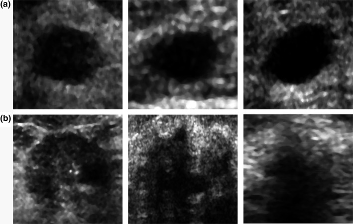
(a) Benign and (b) malignant ultrasound images from the main dataset after the preprocessing.

2.B.1. Neural feature extraction

We implemented two efficient neural feature extraction methods employed in a recent paper.¹⁹ First, features for classification were extracted from each of five max pooling (MP) layers of the original VGG19 model.³⁷ Next, features corresponding to each block were averaged along spatial dimensions and normalized using l ² norm. Features vectors corresponding to each block were then combined to form the final MP feature vector. Second, we additionally used the first FC layer to extract features. For both methods, all zero variance features in respect to the training set were discarded. For classification, we employed the support vector machine (SVM) algorithm.³⁹ In our study, we applied two different approaches to model development. The main dataset was divided into training, validation, and test sets. Training and validation sets were used to determine the best performing hyper‐parameters and the optimal kernel of the SVM classifier via the grid search algorithm. For the C and γ parameters of the SVM algorithm, the grid included parameters in range of [0.00001, 0.0001, …, 1, 10] and [1, 5, …, 100]. The parameter grid also included the kernels, namely the linear and radial basis function kernels. Next, the best performing model was evaluated on the test set. However, the UDIAT and OASBUD datasets are too small to divide them into three separate sets in a convenient way. Therefore, we applied tenfold cross‐validation (case‐based) to evaluate the classification. Within each fold, additional fivefold cross‐validation was used to find optimal hyper‐parameters of the SVM classifiers. To address the problem of class imbalance, we employed class weights inversely proportional to class frequencies in the training set. The SVM classifiers were developed and evaluated using the augmented datasets. To determine a posteriori probability that a mass in the test set is malignant, we averaged the probabilities calculated for each image of this particular mass. Next, to assess the classification performance we determined the receiver operating characteristic (ROC) and calculated the area under the ROC curve (AUC). Sensitivity, specificity, and accuracy of the better‐performing algorithms were calculated using the ROC curve for the point on the curve that was the closest to (0, 1).⁴⁰ Welch's t‐test at significance level of 0.001 was used to determine whether there is a difference in AUC values. All calculations were performed in Python.

2.B.2. Fine‐tuning

The architecture of the original VGG19 model was modified in order to perform fine‐tuning. Unfortunately, the UDIAT and OASBUD datasets were too small to efficiently fine‐tune the VGG19 model, therefore fine‐tuning was employed only in the case of the main dataset. The way to modify the architecture was determined using the validation set. The original FC layers, developed for the ImageNet classes, were replaced with a FC layer with 4096 units followed by a FC layer with 256 units and a single unit employing sigmoid activation function suitable for binary classification (in this case, benign or malignant). For the first two FC layers, we used a rectifier activation functions. Initial weights of the layers were set using the Xavier uniform initializer. With the use of the validation dataset, we found that the highest performance can be obtained if the first four convolutional blocks are frozen and only the fifth block and the fully connected layers are fine‐tuned. We also found that the fine‐tuning of the first convolutional block does not improve the classification performance. To fine‐tune the VGG19 neural network, we used the mini‐batch stochastic gradient descent with Nesterov update. The learning rate was initially set to 0.001 and was decreased by 0.00001 per epoch up to 0.00001. The momentum and the batch size were set to 0.9 and 40, respectively. The binary cross‐entropy loss was employed with weights inversely proportional to class frequencies in the training set. To reduce over‐fitting, we applied dropout with 80% dropout probability to the first fully connected layer. The experiments were performed on a computer equipped with a GeForce GTX 1080 Ti graphics card. The AUC value on the validation set was monitored during the training. As in the case of the SVM algorithm, we selected the model that maximized the AUC value on the validation set.

2.C. Matching layer

Recently proposed CNN‐based breast mass classification approaches employed grayscale US images as input to the pretrained models.^{19, 20, 21, 22} In this paper, we propose to adjust the grayscale US images to the pretrained model instead of duplicating grayscale images across the channels or modifying the first convolutional layer of the CNN. By performing this transformation, we aim to utilize more efficiently the representational capacity of the deep model. For this task, we use a ML that transforms the input grayscale images to RGB images via a linear transformation:

$${\mathit{I}}_{\mathit{o}ut}=\overrightarrow{\mathit{a}}{\mathit{I}}_{\mathit{i}n}+\overrightarrow{\mathit{b}}$$

where ${\mathit{I}}_{\mathit{i}n}$ is the grayscale image, ${\mathit{I}}_{\mathit{o}ut}$ is the output RGB image, $\overrightarrow{\mathit{a}}$ and $\overrightarrow{\mathit{b}}$ are the transformation parameters that shall be determined during training. This transformation is a one‐dimensional (1D) convolution with a bias term. One‐dimensional convolutions were employed, for example, by the authors of the GoogleLeNet CNN to reduce the dimensionality of the input data.³¹ In our case, we use a 1D convolution layer to artificially increase the dimensions of the input images and ideally perform color conversion from gray level images to RGB. Figure 2 depicts the modified VGG19 architecture that includes the ML layer in the front. In this study, we determined the parameters of the ML during fine‐tuning using the back‐propagation algorithm in a way that minimizes the loss function.

Figure 2.

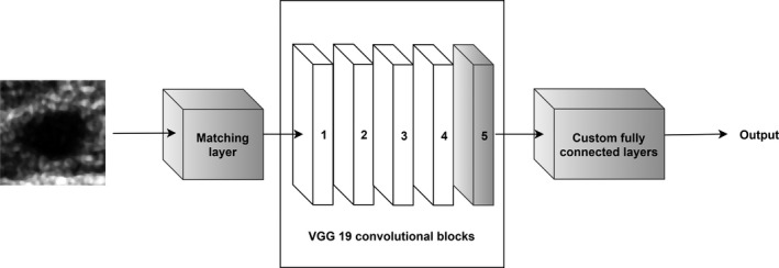
The modified architecture of the VGG19 CNN, gray colors indicate the trainable layers. We propose to add a ML in front of the pretrained model to transform the grayscale US images to RGB to utilize more efficiently the representation capacity of the deep model.

3. Results

First, we used the grayscale images to perform classification of the B‐mode images from the main dataset following the standard approach.^{19, 20, 22, 25} For each US image, the gray level intensities were copied to RGB channels and the VGG19 CNN was tuned. The highest AUC value on the validation set, equal to 0.921, was obtained after 16th epoch. The corresponding AUC value on the test set was equal to 0.895. Next, we extracted the MP and FC features using the original VGG19 model and used those features to train the SVM classifiers. The validation set was employed to select the best hyper‐parameters. For both feature sets, we obtained similar AUC values equal to 0.849 on the test set. The classification performance is depicted in Table 1 and the ROC curves are shown in Fig. 3.

Table 1.

Classification performance of the models developed without the ML for our dataset. The standard deviations of the parameters were calculated using bootstrap

Method	AUC	Accuracy	Sensitivity	Specificity
Fine‐tuning	0.895 ± 0.031	0.860 ± 0.024	0.848 ± 0.056	0.863 ± 0.026
MP features	0.849 ± 0.036	0.793 ± 0.036	0.757 ± 0.054	0.803 ± 0.048
FC features	0.849 ± 0.036	0.800 ± 0.038	0.757 ± 0.054	0.812 ± 0.046
Fine‐tuning, ML	0.936 ± 0.019	0.887 ± 0.028	0.848 ± 0.039	0.897 ± 0.035
MP features, ML	0.889 ± 0.029	0.860 ± 0.044	0.757 ± 0.058	0.889 ± 0.062
FC features, ML	0.873 ± 0.036	0.753 ± 0.044	0.879 ± 0.058	0.718 ± 0.053

Figure 3.

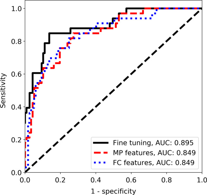
The ROC curves for the CNN‐based classification without the ML in the case of the main dataset. [Color figure can be viewed at wileyonlinelibrary.com]

Next, we fine‐tuned the VGG19 CNN combined with the ML using the back‐propagation algorithm. The highest AUC value on the validation set, equal to 0.961, was obtained after 7th epoch and corresponded to AUC value of 0.936 on the test set, see Table 2 and Fig. 4. To visualize how the ML works, we converted two grayscale US images into RGB images with results depicted in Fig. 5. Following the conversion, the image was dominated by light blue and yellow colors.

Table 2.

Classification performance of the models developed with and without the ML in the case of the UDIAT and OASBUD datasets. The standard deviations of the parameters were calculated using bootstrap

Dataset	Method	AUC	Accuracy	Sensitivity	Specificity
UDIAT	MP features	0.858 ± 0.029	0.853 ± 0.024	0.796 ± 0.043	0.880 ± 0.027
	FC features	0.849 ± 0.031	0.822 ± 0.037	0.759 ± 0.043	0.853 ± 0.053
	MP features, ML	0.873 ± 0.027	0.840 ± 0.023	0.833 ± 0.037	0.844 ± 0.027
	FC features, ML	0.893 ± 0.030	0.840 ± 0.024	0.851 ± 0.042	0.834 ± 0.030
OASBUD	MP features	0.819 ± 0.030	0.760 ± 0.029	0.692 ± 0.057	0.833 ± 0.057
	FC features	0.791 ± 0.035	0.750 ± 0.031	0.750 ± 0.044	0.750 ± 0.050
	MP features, ML	0.831 ± 0.031	0.760 ± 0.031	0.762 ± 0.059	0.750 ± 0.061
	FC features, ML	0.881 ± 0.023	0.830 ± 0.026	0.807 ± 0.039	0.854 ± 0.036

Figure 4.

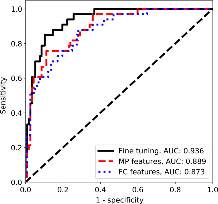
The ROC curves for the CNN‐based classification with the ML in the case of the main dataset. [Color figure can be viewed at wileyonlinelibrary.com]

Figure 5.

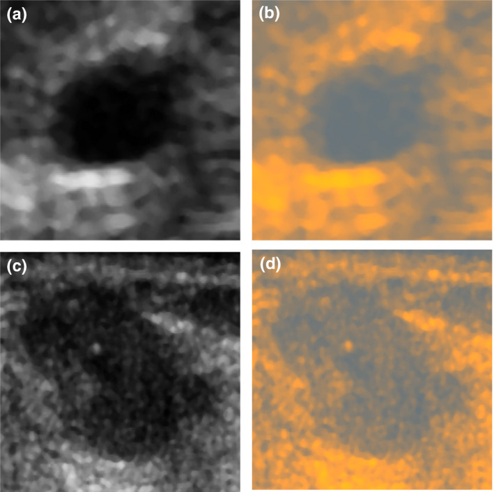
Conversion of grayscale US images from our dataset to RGB using the ML, (a) a benign lesion image and (b) its conversion, (c) a malignant lesion image and (d) its conversion. By using the color conversion, it was possible to more efficiently use the CNN model pretrained on RGB images. [Color figure can be viewed at wileyonlinelibrary.com]

The converted RGB US images were utilized to extract the MP and FC features using the original VGG19 model (not fine‐tuned). Again, the validation set was employed to find the best performing hyper‐parameters for the SVM classifiers. For the RGB images, we obtained higher AUC values on the validation and the test set, equal to 0.889 and 0.873 for the MP and FC features, respectively. Color conversion improved the classification performance. In comparison to gray US images, the AUC values significantly increased by around 0.04 (P < 0.001), see Table 1. The ROC curves calculated for the classifiers developed using the ML layer are depicted in Fig. 4.

In the next step, we extracted the MP and FC features from the VGG19 model using the B‐mode images from the UDIAT and OASBUD datasets. For each US image, the gray level intensities were copied to RGB channels. In the case of the UDIAT dataset, we obtained AUC values of 0.858 and 0.849 for the MP and FC features, respectively. For the OASBUD dataset, the corresponding AUC values for the MP and FC features were equal to 0.819 and 0.791, respectively. Unfortunately, due to small sizes of these datasets we were not able to perform fine‐tuning in an efficient way, so we employed the ML developed using the main dataset. As in the case of our dataset, all B‐mode images from the UDIAT and OASBUD datasets were converted to RGB using the ML and utilized to extract the FC and the ML features. The same cross‐validation folds were used to evaluate the performance. Results showed that due to the color conversion the classification performance increased. For the UDIAT dataset, the AUC values for the MP and FC features increased to 0.873 and 0.893, respectively. In the case of the OASBUD, the AUC values were equal to 0.831 and 0.881 for the MP and FC features, respectively. The ML improved significantly the AUC values (P < 0.001) in the case of the FC features (both datasets). However, for the classifiers trained using the MP features the improvement was too small to provide statistically significant difference. Results are depicted in Table 2. Figure 6 shows how the ML converts the B‐images from the UDIAT and OASBUD datasets to RGB.

Figure 6.

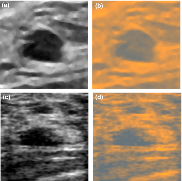
(a) Image from the UDIAT dataset and (b) its conversion to RGB, (c) image from the OASBUD and (d) its conversion to RGB. By using the color conversion, it was possible to more efficiently use the CNN model pretrained on RGB images. [Color figure can be viewed at wileyonlinelibrary.com]

Four radiologists participated in our study. Table 3 shows the distribution of the BI‐RADS categories for the masses in the test set. The Fleiss’ kappa was equal to 0.41 indicating moderate agreement of the radiologists in BI‐RADS category final assessment. Table 4 presents the classification performance of the radiologists employing the BI‐RADS categories. The AUC values ranged between 0.806 and 0.882 with mean of 0.849. The AUC value for the better‐performing CNN with ML was significantly higher than the highest AUC value for the radiologists, 0.936 vs 0.882 (P < 0.001). Accuracy, sensitivity, and specificity were determined for the BI‐RADS category 3 (probably benign) used as the benign cutoff. In this case, the sensitivity of the radiologists was excellent (mean 0.992), but the specificity was lower (mean 0.412), indicating an expected bias toward not missing a positive mass. To additionally compare the assessment of the radiologists with our better‐performing method, we employed the following procedure. First, majority voting was applied to assign a single BI‐RADS category to each breast mass. Ties were handled by assigning the higher BI‐RADS category. Second, we investigated the relation between the output of the network (a posteriori probability of malignancy) and the BI‐RADS category (after voting) assigned to each mass. Figure 7 shows that the probability of malignancy increases with the BI‐RADS category, as expected. To confirm this observation, the Mann–Whitney statistical tests with Bonferroni correction were applied. Results show that four groups are statistically different (P < 0.05), expect for the BI‐RADS categories 2 and 3 (P = 0.22). These two groups contained only benign lesions for which the network assigned small probabilities of malignancy.

Table 3.

Distribution of the BI‐RADS categories for the test set, Fleiss’ kappa was equal to 0.41

	BI‐RADS
	2	3	4	5
Radiologist 1
Benign	44	15	57	1
Malignant	0	1	23	9
Radiologist 2
Benign	37	13	64	3
Malignant	0	0	16	17
Radiologist 3
Benign	41	11	61	4
Malignant	0	0	12	21
Radiologist 4
Benign	19	13	60	25
Malignant	0	0	3	30

Table 4.

Performance of the radiologists employing BI‐RADS for the benign cutoff set to BI‐RADS 3

	AUC	Accuracy	Sensitivity	Specificity
Radiologist 1	0.806 ± 0.028	0.607	0.967	0.504
Radiologist 2	0.848 ± 0.028	0.553	1	0.427
Radiologist 3	0.882 ± 0.026	0.567	1	0.444
Radiologist 4	0.860 ± 0.027	0.433	1	0.273
Mean	0.849	0.540	0.992	0.412

Figure 7.

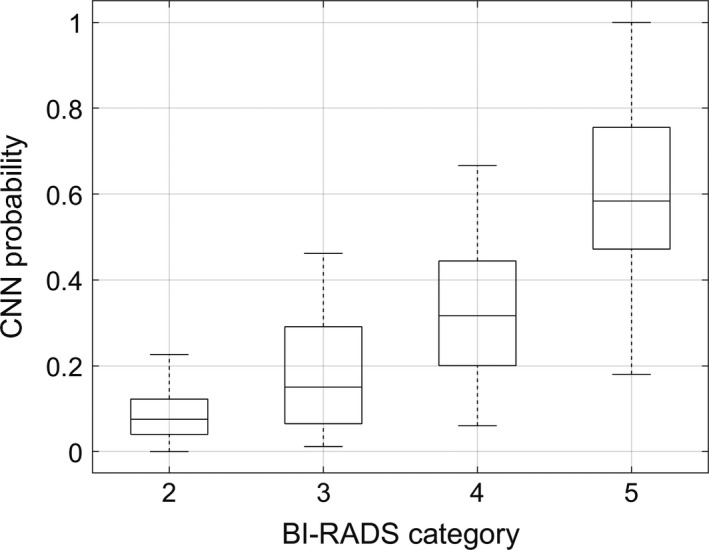
Relation between the output of the CNN with the ML and the average BI‐RADS category assigned to each breast mass by the radiologists.

To illustrate the examples that were difficult for our better‐performing model to classify (fine‐tuned VGG19 model with the ML), we extracted from the test set the images of malignant and benign breast masses that were assessed with the highest and the lowest confidence level for each class, these are shown in Fig. 8. For example, Fig. 8(b) shows a benign mass that was assessed with the highest confidence of being malignant by the classifier. For this mass, the radiologists assigned BI‐RADS categories 4, 4, 4 and 5, which indicates that according to the radiologists this mass was suspicious for malignancy. Figure 8(d) depicts a malignant mass that was assessed with the lowest confidence of being malignant by the classifier. All radiologists assigned BI‐RADS category 5 to this mass. The oval shape, moderate posterior enhancement and fairly uniform anechoic pattern of this mass might be the reason why the model performed worse in this case.

Figure 8.

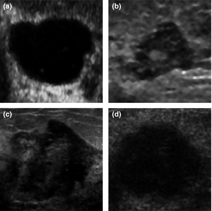
Benign masses assessed by the fine‐tuned model as malignant with (a) the lowest (a posteriori probability of 0.98, BI‐RADS: 2, 2, 2, 2) and (b) the highest confidence level (a posteriori probability of 0, BI‐RADS 4, 4, 4, 5), and malignant masses assessed as malignant with (c) the highest (a posteriori probability of 1, BI‐RADS: 4, 5, 5, 5) and (d) the lowest confidence level (a posteriori probability of 0.33, BI‐RADS 5, 5, 5, 5).

4. Discussion

Our study demonstrates potential usefulness of a deep CNN‐based approach for breast mass classification in US images on three different datasets. In the case of the main dataset, we evaluated three transfer learning methods and achieved good results with each of them. The highest AUC value of 0.936 was achieved for the fine‐tuned VGG19 model combined with the ML. Using the MP and FC features, we obtained AUCs ranged from 0.849 to 0.889. In the case of the other datasets the AUC values ranged from 0.791 to 0.893. Although we were not able to fine‐tune the model using the smaller datasets, we still obtained similar classification performance using the ML and FC features as in the case of the main dataset. For the UDIAT dataset, the performance was almost the same, while for the OASBUD dataset the AUC values were lower by about 0.03 (without the ML). All these results are comparable with the results reported in previous papers,^{19, 20, 25} where the AUC values of around 0.85 were obtained. In one of the studies, the GoogleLeNet was fine‐tuned to classify breast masses in US images.²¹ The authors achieved high AUC value of 0.96. However, the authors used a large set of over 7000 US images to develop the model. In our case, we used a set of 882 breast mass images to develop the model, which may explain the difference in AUC values. Supposedly, with a larger dataset it is possible to fine‐tune the model in a more efficient way.

In our study, fine‐tuning proved to be more efficient than the SVM algorithm utilizing directly extracted CNN features; we obtained higher AUC values by around 0.04 for the main dataset. The better performance may be partially explained by the fact that we fine‐tuned the last convolutional block of the VGG19 model. The usefulness of the convolutional blocks of the VGG19 CNN for breast mass classification was evaluated separately in one of the previous papers.²⁰ The performance of the last 5th convolutional block was lower than in the case of the 4th block, which suggests that the 5th block is specifically related to recognition of the ImageNet objects. The approach employing fine‐tuning, however, is more challenging and troublesome to develop. It requires to replace the FC layers of the original CNN with custom layers and determining which layers of the original network should be trainable during the fine‐tuning. Moreover, the learning rate and other hyper‐parameters have to be correctly selected to yield good classification performance on the validation set. Iterating over methods of model development is time‐consuming and may not yield good results at first. Moreover, in the case of a small dataset, the fine‐tuning might not be efficient and it is more reasonable to utilize the FC or MP features.

The concept of the color conversion has been widely employed in the image analysis field.⁴¹ Usually, a type of color conversion is used before image segmentation.^{42, 43} In the case of deep learning, color conversion was employed in deep colorization⁴⁴ or neural style transfer.⁴⁵ Our study shows that color distribution appears to be an important factor and that it should be taken into account to more efficiently use transfer learning with pretrained deep models. By utilizing the ML, we were able to obtain better classification performance. The first layers of the pretrained network commonly include color blob detectors. Modifying these layers may not necessarily lead to better performance, because those layers are somehow connected with the deeper layers in the network. With the color conversion, it was possible to more efficiently use the pretrained CNN. This advantage is clearly depicted in the case of the MP and FC features extracted from all datasets. The ML developed using the main dataset proved to work with other datasets as well. This shows the universality of our approach. For example, in the case of the FC features extracted using the OASBUD dataset due to the color conversion the AUC value increased from 0.791 to 0.881. Moreover, the color conversion enabled us to more efficiently fine‐tune the VGG19 CNN. In this work, we used linear transformations to convert grayscale US images to RGB. Regular image preprocessing required in the case of the VGG19 network could be performed using only the bias term $\overrightarrow{\mathit{b}}$. We decided to additionally employ the scaling parameter $\overrightarrow{\mathit{a}}$ for several reasons. First, color inversion in particular channels may improve the performance. Second, the area of mass in US image is commonly hypoechoic or anechoic while the surrounding tissue is significantly brighter. For the network to perform well, it might be useful to rescale this relation and for example decrease this difference in brightness levels. The proposed approach, however, is general and not limited to grayscale images or to US, so it can be applied to RGB images as well. Moreover, it is possible to use other transformations including nonlinear ones, which could be useful for processing images from different medical modalities. The advantage of our approach is that the transformation is determined during fine‐tuning automatically. In some sense, our approach can be perceived as adding an additional neural network in front of the pretrained one. The main issue is that the transformation may change the range of intensities to one outside [0, 255] making the transformed image difficult or impossible to visualize.

The CNN‐based methods developed using the main dataset achieved results comparable to or higher than the AUC obtained by the radiologists. Our best performing approach showed an AUC value that was higher by 0.04 to 0.13 than the range of AUCs calculated for the radiologists. These results demonstrate potential clinical usefulness of the developed classifiers. However, it is important to recognize that diagnostic breast US is commonly used to determine whether and where to perform the biopsy rather than to determine if a lesion is benign or malignant. In order to avoid missing a potential malignancy, radiologists achieve very high sensitivity at the expense of lower specificity.³⁴ The better classifier in this study achieved higher specificity (0.90) but lower sensitivity (0.85) than all of the radiologists. However, according to the ROC curve in Fig. 4, at the sensitivity of 1.0 our better performing CNN achieves higher specificity of 0.65 than the radiologists (0.3‐0.5). We also showed that the output of the better‐performing model (a posteriori probability of malignancy) is related to the BI‐RADS category. This, however, was expected since both measures aim to assess the level of malignancy.

To more thoroughly evaluate the classifier utility in a clinical environment, it will be desirable to employ the CNN as a decision tool with the radiologist “in the loop.” For a particular mass, the CNN result may be overridden by the interpreting radiologist in the final assessment. The current results do not describe a complete medical device ready for clinical use but they may provide necessary information to properly design and study such a tool. In our approach, the radiologists identify the mass and select an ROI, hence requiring interaction by the radiologist. It remains to be seen if this can be done efficiently or semiautomatically without impacting workflow, and if it is useful for the radiologist with difficult cases where accurate assessment of the type of breast mass is desired. In future, it would be also interesting to investigate whether the CNNs can be used to classify malignant and benign breast mass subtypes.

5. Conclusion

In this study, we utilized the VGG19 CNN for breast mass classification and introduced the concept of the matching layer, a layer that is used to convert gray scale ultrasound images to RGB. We demonstrated that with the ML it was possible to perform more efficient classification than in the case of duplicating grayscale US images across the RGB channels. The concept of the ML is general and can be applied to various problems to enhance CNN‐based transfer learning techniques. The AUC obtained for our better‐performing classifier was higher than that of four expert radiologists who utilized BI‐RADS lexicon and categories. Even at sensitivity of 1.0, the classifier achieved higher specificity in comparison to the radiologists. In future, we are going to perform additional studies to determine the clinical usefulness of the employed methods.

Conflict of interest

The authors have no conflicts to disclosure.

References

- 1. Bray F, Ferlay J, Soerjomataram I, Siegel RL, Torre LA, Jemal A. Global cancer statistics 2018: GLOBOCAN estimates of incidence and mortality worldwide for 36 cancers in 185 countries. CA Cancer J Clin. 2018;68:394–424. [DOI] [PubMed] [Google Scholar]
- 2. Bott R. ACR BI‐RADS Atlas; 2014. 10.1007/s13398-014-0173-7.2 [DOI]
- 3. Berg WA, Blume JD, Cormack JB, et al. Combined screening with ultrasound and mammography vs mammography alone in women at elevated risk of breast cancer. JAMA. 2008;299:2151–2163. [DOI] [PMC free article] [PubMed] [Google Scholar]
- 4. Hooley RJ, Greenberg KL, Stackhouse RM, Geisel JL, Butler RS, Philpotts LE. Screening US in patients with mammographically dense breasts: initial experience with Connecticut Public Act 09‐41. Radiology. 2012;265:59–69. [DOI] [PubMed] [Google Scholar]
- 5. Cheng HD, Shan J, Ju W, Guo Y, Zhang L. Automated breast cancer detection and classification using ultrasound images: a survey. Pattern Recognit. 2010;43:299–317. [Google Scholar]
- 6. Flores WG, de Albuquerque Pereira WC, Infantosi AFC. Improving classification performance of breast lesions on ultrasonography. Pattern Recognit. 2015;48:1125–1136. [Google Scholar]
- 7. Giger ML, Karssemeijer N, Schnabel JA. Breast image analysis for risk assessment, detection, diagnosis, and treatment of cancer. Annu Rev Biomed Eng. 2013;15:327–357. [DOI] [PubMed] [Google Scholar]
- 8. André MP, Galperin M, Berry A, et al. Performance of a method to standardize breast ultrasound interpretation using image processing and case‐based reasoning. In: André M, Jones J, Lee H, eds. Acoustical Imaging. Dordrecht: Springer; 2011:3–9. [Google Scholar]
- 9. Bian C, Lee R, Chou Y‐H, Cheng J‐Z. Boundary regularized convolutional neural network for layer parsing of breast anatomy in automated whole breast ultrasound. In: Descoteaux M, Maier‐Hein L, Franz A, Jannin P, Collins D, Duchesne S, eds. International Conference on Medical Image Computing and Computer‐Assisted Intervention. Cham: Springer; 2017:259–266. [Google Scholar]
- 10. Chen C‐M, Chou Y‐H, Han K‐C, et al. Breast lesions on sonograms: computer‐aided diagnosis with nearly setting‐independent features and artificial neural networks. Radiology. 2003;226:504–514. [DOI] [PubMed] [Google Scholar]
- 11. Cheng J‐Z, Chou Y‐H, Huang C‐S, et al. Computer‐aided US diagnosis of breast lesions by using cell‐based contour grouping. Radiology. 2010;255:746–754. [DOI] [PubMed] [Google Scholar]
- 12. Cheng J‐Z, Ni D, Chou Y‐H, et al. Computer‐aided diagnosis with deep learning architecture: applications to breast lesions in US images and pulmonary nodules in CT scans. Sci Rep. 2016;6:24454. [DOI] [PMC free article] [PubMed] [Google Scholar]
- 13. Drukker K, Gruszauskas NP, Sennett CA, Giger ML. Breast US computer‐aided diagnosis workstation: performance with a large clinical diagnostic population. Radiology. 2008;248:392–397. [DOI] [PMC free article] [PubMed] [Google Scholar]
- 14. Joo S, Yang YS, Moon WK, Kim HC. Computer‐aided diagnosis of solid breast nodules: use of an artificial neural network based on multiple sonographic features. IEEE Trans Med Imaging. 2004;23:1292–1300. [DOI] [PubMed] [Google Scholar]
- 15. Shen WC, Chang RF, Moon WK, Chou YH, Huang CS. Breast ultrasound computer‐aided diagnosis using BI‐RADS features. Acad Radiol. 2007;14:928–939. [DOI] [PubMed] [Google Scholar]
- 16. Hoda N, Hamid F, Nasrin A, Alejandro F, Ali G. Classification of breast lesions in ultrasonography using sparse logistic regression and morphology‐based texture features. Med Phys. 2018;45:4112–4124. [DOI] [PubMed] [Google Scholar]
- 17. Hu Y, Qiao M, Guo Y, et al. Reproducibility of quantitative high‐throughput BI‐RADS features extracted from ultrasound images of breast cancer. Med Phys. 2017;44:3676–3685. [DOI] [PubMed] [Google Scholar]
- 18. Rodriguez‐Cristerna A, Guerrero‐Cedillo CP, Donati‐Olvera GA, Gómez‐Flores W, Pereira WCA. Study of the impact of image preprocessing approaches on the segmentation and classification of breast lesions on ultrasound. In: 2017 14th International Conference On Electrical Engineering, Computing Science and Automatic Control (CCE); 2017:1–4.
- 19. Antropova N, Huynh BQ, Giger ML. A deep feature fusion methodology for breast cancer diagnosis demonstrated on three imaging modality datasets. Med Phys. 2017;44:5162–5171. [DOI] [PMC free article] [PubMed] [Google Scholar]
- 20. Byra M. Discriminant analysis of neural style representations for breast lesion classification in ultrasound. Biocybern Biomed Eng. 2018;38:684–690. [Google Scholar]
- 21. Han S, Kang H‐K, Jeong J‐Y, et al. A deep learning framework for supporting the classification of breast lesions in ultrasound images. Phys Med Biol. 2017;62:7714. [DOI] [PubMed] [Google Scholar]
- 22. Yap MH, Goyal M, Osman F, et al. End‐to‐end breast ultrasound lesions recognition with a deep learning approach. In: Medical Imaging 2018: Biomedical Applications in Molecular, Structural, and Functional Imaging. Vol. 10578; 2018:1057819.
- 23. Xie X, Shi F, Niu J, Tang X. Breast ultrasound image classification and segmentation using convolutional neural networks. In: Hong R, Cheng W‐H, Yamasaki T, Wang M, Ngo C‐W, eds. Advances in Multimedia Information Processing – PCM 2018. Cham: Springer International Publishing; 2018:200–211. [Google Scholar]
- 24. Xu Y, Wang Y, Yuan J, Cheng Q, Wang X, Carson PL. Medical breast ultrasound image segmentation by machine learning. Ultrasonics. 2019;91:1–9. [DOI] [PubMed] [Google Scholar]
- 25. Huynh B, Drukker K, Giger M. MO‐DE‐207B‐06: computer‐aided diagnosis of breast ultrasound images using transfer learning from deep convolutional neural networks. Med Phys. 2016;43:3705. [Google Scholar]
- 26. Yap MH, Pons G, Marti J, et al. Automated breast ultrasound lesions detection using convolutional neural networks. IEEE J Biomed Heal Inform. 2018;22:1218–1226. [DOI] [PubMed] [Google Scholar]
- 27. Zhang Q, Xiao Y, Dai W, et al. Deep learning based classification of breast tumors with shear‐wave elastography. Ultrasonics. 2016;72:150–157. [DOI] [PubMed] [Google Scholar]
- 28. Deng J, Dong W, Socher R, Li L‐J, Li K, Fei‐Fei L. Imagenet: a large‐scale hierarchical image database. In: IEEE Conference on Computer Vision and Pattern Recognition, 2009. CVPR 2009; 2009:248–255.
- 29. Simonyan K, Zisserman A. Very deep convolutional networks for large‐scale image recognition; 2014. arXiv Prepr arXiv14091556.
- 30. Szegedy C, Ioffe S, Vanhoucke V, Alemi AA. Inception‐v4, inception‐resnet and the impact of residual connections on learning. In: Proceedings of the Thirty‐First AAAI Conference on Artificial Intelligence; 2017.
- 31. Szegedy C, Liu W, Jia Y, et al. Going deeper with convolutions. In: Proceedings of the IEEE Conference on Computer Vision and Pattern Recognition; 2015:1–9.
- 32. Piotrzkowska‐Wróblewska H, Dobruch‐Sobczak K, Byra M, Nowicki A. Open access database of raw ultrasonic signals acquired from malignant and benign breast lesions. Med Phys. 2017;44:6105–6109. [DOI] [PubMed] [Google Scholar]
- 33. Byra M, Nowicki A, Wróblewska‐Piotrzkowska H, Dobruch‐Sobczak K. Classification of breast lesions using segmented quantitative ultrasound maps of homodyned K distribution parameters. Med Phys. 2016;43:5561–5569. [DOI] [PubMed] [Google Scholar]
- 34. Dobruch‐Sobczak K, Piotrzkowska‐Wróblewska H, Roszkowska‐Purska K, Nowicki A, Jakubowski W. Usefulness of combined BI‐RADS analysis and Nakagami statistics of ultrasound echoes in the diagnosis of breast lesions. Clin Radiol. 2017;72:339.e7–339.e15. [DOI] [PubMed] [Google Scholar]
- 35. Abadi M, Barham P, Chen J, et al. TensorFlow: a system for large‐scale machine learning. In: OSDI. Vol. 16; 2016:265–283.
- 36. Litjens GJS, Kooi T, Bejnordi BE, et al. A survey on deep learning in medical image analysis. CoRR; 2017; abs/1702.0. http://arxiv.org/abs/1702.05747. [DOI] [PubMed]
- 37. Zheng L, Zhao Y, Wang S, Wang J, Tian Q. Good practice in CNN feature transfer; 2016. arXiv Prepr arXiv160400133.
- 38. Landini L, Sarnelli R. Evaluation of the attenuation coefficients in normal and pathological breast tissue. Med Biol Eng Comput. 1986;24:243–247. [DOI] [PubMed] [Google Scholar]
- 39. Chang C‐C, Lin C‐J. LIBSVM: a library for support vector machines. ACM Trans Intell Syst Technol. 2011;2:27. [Google Scholar]
- 40. Fawcett T. An introduction to ROC analysis. Pattern Recognit Lett. 2006;27:861–874. [Google Scholar]
- 41. Faridul HS, Pouli T, Chamaret C, et al. Colour mapping: a review of recent methods, extensions and applications. In: Computer Graphics Forum. Vol. 35; 2016:59–88.
- 42. Khattab D, Ebied HM, Hussein AS, Tolba MF. Color image segmentation based on different color space models using automatic GrabCut. Sci World J. 2014;2014:1–10. [DOI] [PMC free article] [PubMed] [Google Scholar]
- 43. Sanchez‐Cuevas MC, Aguilar‐Ponce RM, Tecpanecatl‐Xihuitl JL. A comparison of color models for color face segmentation. Procedia Technol. 2013;7:134–141. [Google Scholar]
- 44. Cheng Z, Yang Q, Sheng B. Deep colorization. In: Proceedings of the IEEE International Conference on Computer Vision; 2015:415–423.
- 45. Gatys LA, Ecker AS, Bethge M, Hertzmann A, Shechtman E. Controlling perceptual factors in neural style transfer. In: IEEE Conference on Computer Vision and Pattern Recognition (CVPR); 2017.