Reconstruction of evolving gene variants and fitness from short sequencing reads

Abstract

Directed evolution can generate proteins with tailor-made activities. However, full-length genotypes, their frequencies, and fitnesses are difficult to measure for evolving gene-length biomolecules using most high-throughput DNA sequencing methods as short read lengths can lose mutation linkages in haplotypes. We present Evoracle, a machine learning method that accurately reconstructs full-length genotypes (R² = 0.94) and fitness using short-read data from directed evolution experiments, with substantial improvements over related methods. We validate Evoracle on phage-assisted continuous evolution (PACE), phage-assisted non-continuous evolution (PANCE) of adenine base editors, and OrthoRep evolution of drug-resistant enzymes. Evoracle retains strong performance (R² = 0.86) on data with complete linkage loss between neighboring nucleotides and large measurement noise such as pooled Sanger sequencing data (~$10/timepoint), and broadens the accessibility of training machine learning models on gene variant fitnesses. Evoracle can also identify high-fitness variants, including low-frequency ‘rising stars’, well before they are identifiable from consensus mutations.

Introduction

The generation of peptide, enzymes, proteins and pathways with enhanced or modified activity has contributed to substantial scientific and therapeutic advances^1–4. Directed evolution is a powerful approach that harnesses iterated cycles of mutagenic replication under selection pressure to generate variant molecules with novel activities^5,6. While the directed evolution of modest-length biopolymers such as antibody fragments⁷, peptides⁸, and highly functionalized nucleic acid polymers^9,10 has substantial therapeutic and scientific interest, the directed evolution of gene-length or longer biomolecules can provide access to a larger diversity of activities, such as expanding the targeting capacity of Cas9^11,12, thwarting evolved insecticide resistance³, and developing novel adeno-associated virus tropisms to target therapeutically relevant organs².

Characterizing the evolutionary histories of full-length genotypes that emerge from directed evolution campaigns reveals the solution space that has been explored and can suggest individual mutations for reversion analysis. Understanding epistatic interactions between distant residues can provide insights into the biochemical underpinnings of evolved activity and facilitate reversion analysis. Estimating fitness of full-length gene variants enables the comparison of distinct solutions, allows researchers to prioritize variants for low-throughput follow-up studies, and facilitates optimization of desired activities.

However, monitoring and characterizing key aspects of directed evolution campaigns—including full-length genotypes and their frequencies, evolutionary trajectories, and fitnesses—remains a challenge, especially for genes of typical length and other long biomolecules. Timepoints of directed evolution campaigns can contain enormous genotype diversity (>10⁷ gene variants)^5,6,13. While individual gene variants can be sequenced by shotgun sequencing and overlap graph-based contig assembly^14,15, these approaches scale poorly when tasked on the expansive diversity of genotypes generated by directed evolution. Highly diverse gene pools from directed evolution experiments are commonly subjected to high-throughput sequencing by Illumina methods,¹⁶ but the resulting read lengths are much shorter than most gene lengths, resulting in a loss of associations between non-proximal mutations within individual gene variants. While long-read high-throughput sequencing can address these problems^3,17,18, these approaches are much less available compared to low-throughput Sanger sequencing¹⁹ or high-throughput short-read Illumina sequencing, and also can suffer from higher error rates¹⁷ that can occlude measurement of mutation frequencies. As a result, it can be difficult to follow genotypes that emerge, flourish, change, or are lost through a directed evolution campaign, even though such genotype dynamics are rich with structure-function information that illuminates how evolving genotypes acquire desired properties.

The problem of reconstructing full-length genotypes from short reads has been considered from a variety of perspectives. Methods for reconstructing viral haplotypes from evolutionary data have been developed¹⁵, but they rely on overlap-based algorithms which exploit the typically short distances between polymorphic alleles in evolving viral genomes, and cannot be used when linkage information between alleles is missing. Methods for metagenomic genome assembly^20,21 address the reconstruction of genomes from mixtures of short sequencing reads, but these methods are not designed for disentangling highly similar genomes and can perform poorly on mixtures of evolving genotypes that typically have >95% similarity²². Separately, the problem of deciphering evolutionary lineages and epistasis from evolutionary data has been considered from various angles. Barcoding approaches can track the trajectories of evolutionary lineages²³, but cannot track individual haplotypes over time. Pseudo-time ordering methods have also been developed to deconvolve single mixed samples into phylogenetic trees²⁴, and methods leveraging evolutionary dynamics can reveal epistasis from data without physical linkage²⁵. However, few methods address overlap-free gene or haplotype reconstruction in the context of evolution^26,27.

Here, we describe Evoracle, a machine learning method that reconstructs full-length genotype frequencies, trajectories, and fitness from short-read sequencing data derived from timepoints during directed evolution campaigns. We use datasets with both long-read and short-read sequencing to evaluate Evoracle and related methods^26–28. We consider two published datasets^3,6 and report a new dataset with full-gene sequencing and short read data in 99 samples spanning 37 timepoints from a directed evolution campaign on TadA, an E. coli tRNA adenosine deaminase that was evolved for the adenine base editor ABE8e²⁹. Evoracle substantially outperforms two related overlap-free gene reconstruction methods^26–28 and retains strong performance with pooled Sanger sequencing data, an inexpensive sequencing approach with substantial noise and loss of linkage between sequenced nucleotides. We further show that Evoracle can propose variants with higher fitness than common approaches that use consensus mutations^{3,5,6,11,12,29–31}. We anticipate that Evoracle (https://github.com/maxwshen/evoracle) will be a valuable tool for the directed evolution community.

Results

Inference using Evoracle

Evoracle is a machine learning method that uses noisy short-read data to infer the parameters and latent state of a non-linear dynamical system. We consider a model including two fundamental aspects of directed evolution: enrichment and depletion of genotypes through natural selection governed by fitness w, and a flexible mutation model that introduces new genotypes, parameterized by a discrete vector z of timepoints when each genotype first enters the population at frequencies s. The state transition process updates genotype frequencies x_t at time t with a standard model of asexual fitness-based natural selection^26,32 as $\frac{\mathit{w}}{{\mathit{w}}^{\mathit{T}}{\mathit{x}}_{\mathit{t}}}\odot {\mathit{x}}_{\mathit{t}}$, then introduces a genotype i to the population at time t at frequency s[i] if z[i] = t. We observe data at T timepoints through a lossy stochastic observation process E[y_t] = Bx_t, where B is a binary matrix that is rank deficient because the dimension of y_t is smaller than x_t, which describes DNA sequencing when reads are shorter than genotypes. Evoracle first proposes full-length genotypes that could exist in the population, then uses noisy short-read data to infer the timepoint frequencies and fitness of these full-length genotypes (see Online Methods for a complete description of our algorithm).

Given y₁, y₂, …, y_T, the inference task is to learn (w, s, z). However, this requires solving an intractable discrete optimization problem over T^G possible discrete z, which often exceeds 10¹⁰⁰ for real data. A common workaround is to parameterize a distribution p(z; ψ) and infer (w, s, ψ). However, computing the data likelihood p(y₁, y₂, …, y_T|ψ) is intractable as it requires summing over z, which prevents the use of maximum likelihood estimation (MLE) or variational inference. Prior work has sidestepped this problem by using MLE on a model with a restricted mutation model²⁶, while Evoracle solves the challenging inference task with z under a flexible mutation model that allows genotypes to enter the population at any timepoint. In practice, this enables Evoracle to better fit data where high-fitness genotypes enter the population at later timepoints, which is often the case in directed evolution^{1,3,5,6,11,29,31} or in data collected over long time periods^3,23.

The insight underlying Evoracle is that we can bypass s and z and directly infer x₁, x₂, …, x_T if they satisfy constraints raised by s, z through the state transition process. The inferred s, z can then be computed from x₁, x₂, …, x_T. The constraints are: 1) each genotype enters the population at an arbitrary inferred frequency at most once, 2) frequencies of present genotypes should be consistent with fitness-based natural selection, and 3) absent genotypes have zero frequency. We satisfy these constraints by distinguishing present and absent genotypes using a small frequency threshold ϵ, renormalizing present frequencies, and enforcing a gradient-matching regularizer on present genotypes to ensure fidelity to the natural selection process. These steps explicitly handle all constraints except ensuring that genotypes enter the population at most once, which is handled implicitly by encouraging fidelity to the natural selection process: in Supplementary Note 1, we prove that in mild conditions, genotype frequencies under natural selection can rise to appreciable frequency at most once.

These insights lead to a simple likelihood-free inference algorithm supporting efficient gradient-based optimization. Evoracle enjoys better efficiency over related approaches including expectation maximization, sequential Monte Carlo^33,34 and approximate Bayesian computation³⁵ (Online Methods). Evoracle’s infers $\widehat{\mathit{w}}$ and ${\widehat{\mathit{x}}}_{\mathit{t}}$ for each t by optimizing a loss function with a data fitting term $D_{KL}(\mathit{B}{\widehat{\mathit{x}}}_{\mathit{t}}\Vert {\mathit{y}}_{\mathit{t}})$ and a gradient-matching^36,37 fidelity term comparing inferred states to the natural selection process ${\mathrm{D}}_{\mathrm{K}\mathrm{L}}\left(\frac{\widehat{\mathit{w}}}{{\widehat{\mathit{w}}}^{\mathit{T}}{\widehat{\mathit{x}}}_{\mathit{t}}}\odot {\widehat{\mathit{x}}}_{\mathit{t}}\Vert {\widehat{\mathit{x}}}_{\mathit{t}+1}\right)$. We designed a regularizer motivated by skew structure induced by our model of natural selection, which sorts genotype frequencies by fitness in logarithmic time, then monotonically increases the unnormalized skew of the genotype frequency distribution. This leads to genotype frequency distributions with high unnormalized skew $\Vert {\mathit{x}}_{\mathit{t}}–1/G{\Vert }_3^3$ (Extended Data Fig. 1). We also prove that the gradient-matching term ${\mathrm{D}}_{\mathrm{K}\mathrm{L}}(\frac{\widehat{\mathit{w}}}{{\widehat{\mathit{w}}}^{\mathit{T}}{\widehat{\mathit{x}}}_{\mathit{t}}}\odot {\widehat{\mathit{x}}}_{\mathit{t}}\Vert {\widehat{\mathit{x}}}_{\mathit{t}+1})$ implicitly encourages a smaller L₁-norm for s, which is compatible with low initial genotype frequencies expected under typical mutation rates^3,6.

The non-identifiability of our measurement process E[y_t] = Bx_t may raise concerns for inference, though regularization can improve identifiability, and Evoracle is consistent and accurate in practice. In Supplementary Note 1, we theoretically investigate the impact of regularizing to a state transition process on identifiability, and prove that the highest fitness genotype is identifiable from partial measurements under mild conditions.

Evoracle’s performance is robust to noise, varying hyperparameters, and genotype proposal strategies (Extended Data Fig. 1–2, Supplementary Note 2). We provide guidelines for using Evoracle to real data in the Online Methods and Supplementary Note 3.

Reconstruction of evolving 2,138-nt genotypes from PACE

We evaluated Evoracle’s ability to reconstruct full-length genotype frequencies from standard 150-nt sequencing data. Cry1Ac (2,138 nt) encodes an insecticidal Bacillus thuringiensis δ-endotoxin (Bt toxin) widely used in agriculture for pest control³. We previously evolved Cry1Ac using phage-assisted continuous evolution (PACE)⁵ to bind a non-native cadherin-like receptor with high affinity (K_d = 18-34 nM), thereby circumventing evolved insect resistance to Bt toxins³. In PACE⁵, the gene of interest is encoded by bacteriophage and its activity is linked to expression of gene III, a gene necessary for phage propagation, by a plasmid-based DNA circuit in host E. coli cells. A mutagenesis plasmid (MP) controls the phage mutation rate. PACE occurs in culture vessels (“lagoons”) continuously diluted with host E. coli cells at rates that allow mutagenic replication of phage, but that are too fast to allow replication of E. coli⁵. During PACE, phage encoding active gene variants replicate faster than they are diluted from the lagoon, while inactive variants fail to generate infectious progeny and are diluted out of the persisting gene population⁵.

We previously evolved Cry1Ac using PACE for 528 h. Over this time, surviving gene variants experienced an average of 511 generations of mutagenic replication and continuous selection across four selection phases, each with a different target protein, selection stringency, and/or lagoon outflow rate³. At 34 timepoints, taken every 12 h or 24 h, lagoon samples were collected and sequenced with long-read (>2,138 nt) PacBio sequencing to an average depth of ~500 reads and short-read (150-nt) Illumina sequencing to an average depth of ~500,000 reads. We identified commonly evolved non-synonymous mutations at 19 positions with high confidence that collectively spanned 658 aa (1,974 nt), and tabulated frequencies of combinations of mutations at these positions within ten 100-nt segments spanned by short reads (Fig. 1B, Online Methods). The trajectories of these 19 mutations were complex: some mutations fixed early, while others rose and fell multiple times (Fig. 1C). We refer to combinations of amino acids at these 19 positions as “full-length genotypes”, although we note that they actually represent mutational families (Online Methods).

Fig. 1 |. Genotype reconstruction during evolution from short-read sequencing data with incomplete physical linkage.

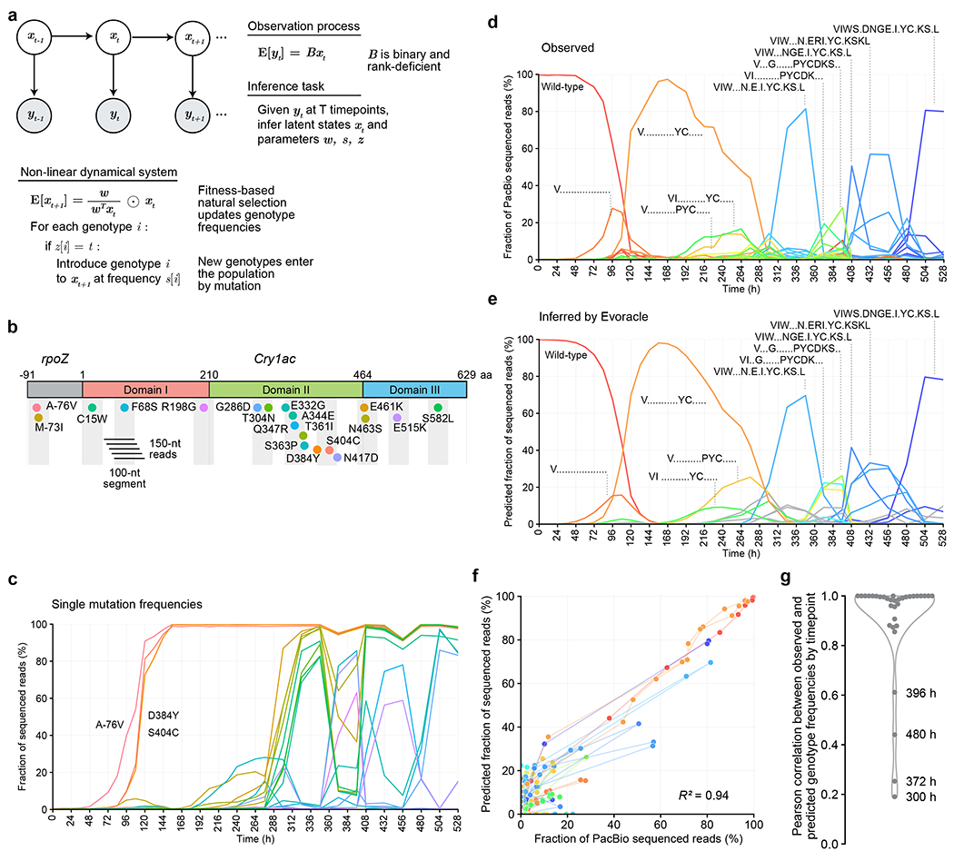
a, Overview of the method. b, Schematic of the Cry1Ac gene (2,138 nt) with locations of 19 major mutations evolved in a previous study³. Gray boxes indicate 100-nt segments measurable from Illumina sequencing data. Colored dots represent amino acid mutations. c, Observed frequencies of 19 major Cry1Ac mutations at 34 timepoints (spanning 528 h) of PACE from short-read DNA sequencing data. Mutation colors match Fig. 1b. d, Observed Cry1Ac (2,138 nt) genotypes from 34 timepoints (spanning 528 h) of PACE from long-read sequencing data. Periods denote wild-type amino acid. Colors represent distinct genotypes. e, Inferred Cry1Ac (2,138 nt) trajectories from 34 timepoints (spanning 528 h) of phage-assisted continuous evolution from 150-nt Illumina sequencing data. Periods represent wild-type amino acids. Gray lines indicate genotypes that are not present in PacBio data. Colors match those in Fig. 1d. f, Consistency between observed and predicted full-length genotype frequencies. Genotypes are colored in the same manner as Fig. 1d, and lines connect genotypes at neighboring timepoints. g, Consistency between observed and predicted full-length genotype frequencies by timepoint with kernel density estimate.

Using only 100-nt reads truncated from PacBio reads, we used Evoracle to infer full-length genotype trajectories throughout the 528 h of PACE. Predicted frequencies closely matched observed frequencies from held-out long-read sequencing data (R² = 0.94; Fig. 1D–G). Inferred fitnesses were also consistent with fitnesses calculated from full-length genotype frequencies from long-read data (the fitness of a genotype is its replication rate relative to other genotypes, R² = 0.71, Online Methods). From 312–528 h, Evoracle accurately reconstructed a complex series of genotypes that featured up to 13 simultaneous mutations spanning 658 aa (1,974 nt) (Fig. 1E), demonstrating effective recovery of distant mutation combinations from short 100-nt read segments. Evoracle also accurately reconstructed the trajectories of several genotypes that peaked at 20% frequency or lower (Fig. 1E), and recognized timepoints with high genotype diversity (Fig. 1E). Reconstruction performance was higher for high-frequency genotypes that are typically of greatest interest, and lower on rarer genotypes, which typically have weaker activity and lower interest (Spearman R = 0.09, P=4.6×10⁻¹⁰). Taken together, Evoracle effectively reconstructs historical trajectories of full-length genotypes that arise during directed evolution from short-read data with missing linkage.

Evoracle’s inferences can enable epistatic analysis of mutations (Online Methods). The triple mutant A-76V, D384Y, S404C dominated the lagoon from 120-288 h, even though it had less fitness than expected from an independent combination of fitnesses from the single mutant A-76V and the double mutant D384Y, S404C according to the long-read sequencing data (Extended Data Fig. 3). Evoracle’s inferred fitnesses recapitulated the same conclusion from short-read sequencing data (Extended Data Fig. 3), identifying D384Y, S404C as driver mutations and A-76V as a passenger mutation.

Fitness reconstruction on OrthoRep data

We next evaluated Evoracle on data from OrthoRep, a separate in vivo continuous directed evolution method⁶. During OrthoRep-mediated evolution, a gene of interest on a linear plasmid undergoes stable mutagenic replication at ~100,000-fold higher mutation rates (to ~1×10⁻⁵ substitutions per base) by a DNA polymerase that acts orthogonally to (does not increase) mutation rates on the host yeast genome⁶. OrthoRep was used to evolve antimalarial drug resistance to pyrimethamine in Plasmodium falciparum malarial dihydrofolate reductases (PfDHFRs)⁶. The OrthoRep study used pooled Sanger sequencing to obtain population sequencing traces that were analyzed by Surveyor³⁸ to estimate position-wise mutation frequencies with complete loss of physical linkage between neighboring nucleotides³⁸. Importantly, Surveyor has a high error rate³⁹: it estimates 95% of frequencies within ±5.7% of Illumina sequencing (standard deviation, s.d. ~3%) and is typically unable to resolve mutation frequencies below 5%. We gathered data from the OrthoRep study⁶ comprising three replicates with timepoints from 14 passages (Online Methods) spanning 87 generations with 5–10 amino acid mutations across the gene (Fig. 2A–C). We also gathered drug resistance measurements of the minimum inhibitory concentration (MIC) for two mutational landscapes with 5 mutations and 32 alleles from the OrthoRep study ⁶.

Fig. 2 |. Evolutionary fitness reconstruction from pooled Sanger sequencing of OrthoRep campaigns.

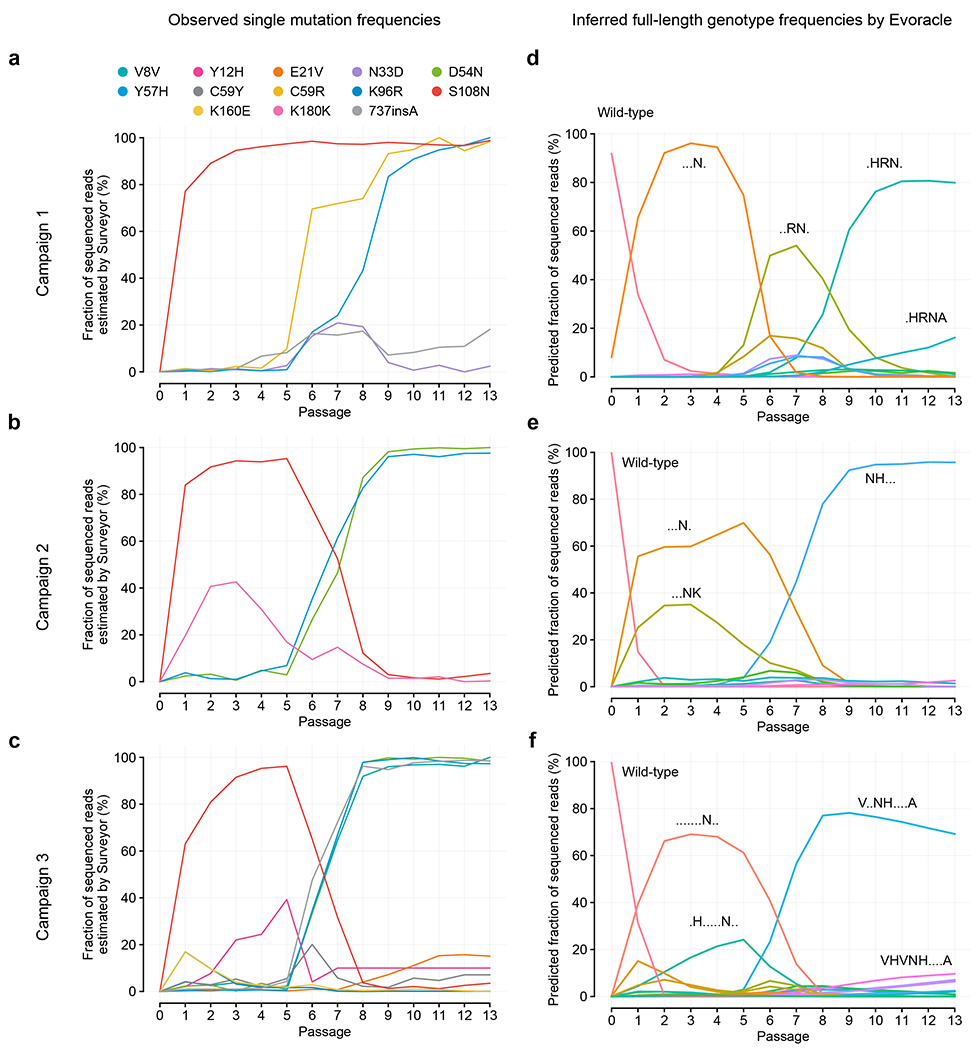
a-c, Point mutation frequencies for three PfDHFR evolution campaigns. Colors represent amino acid mutations. d-f, Inferred full-genotype frequencies for three PfDHFR evolution campaigns. Colors represent full-length genotypes. These genotype trajectories are hypotheses from our model, and are consistent with observed point mutation frequencies.

We used Evoracle to infer the fitness of full-length PfDHFR genotypes from pooled Sanger sequencing data with complete loss of physical linkage (Fig. 2D–F, Extended Data Fig. 3). Across three campaigns, all pairs of full-length genotypes were correctly ordered by reported log₁₀ MIC of pyrimethamine [M] values using inferred fitness values (P = 0.04, N = 5 pairs; Online Methods). These results suggest that Evoracle can accurately distinguish full-length genotypes with weak and strong activity under designed selections from pooled Sanger sequencing data at different time points during evolution.

Reconstruction of base editor variants from PACE and PANCE

TadA (167 amino acids) is a tRNA adenosine deaminase in E. coli that converts adenine to inosine.⁴⁰ We previously evolved TadA mutants that deaminate deoxyadenosine to create adenine base editors (ABEs) such as ABE7.10⁴¹. More recently, the TadA from ABE7.10 (TadA-7.10) was further evolved to yield ABE8e²⁹, which has 590-fold increased activity (k_app), improved editing efficiency, and eight non-synonymous mutations relative to TadA-7.10 (22 non-synonymous mutations from wild-type TadA). The ABE8e directed evolution campaign began with two parallel phage-assisted non-continuous evolution (PANCE) campaigns across 15 overnight serial passages. PANCE operates similarly to PACE, except continuous dilution of phage is replaced by manual passaging into fresh host-cell culture after a user-defined time period. PANCE is less stringent than PACE due to its lower effective dilution rate. Final aliquots from these low-stringency PANCEs were then used to seed four parallel high-stringency PANCE experiments for 10 further passages, which were finally seeded into three parallel PACE lagoons that ran for 84 h (Extended Data Fig. 4)²⁹. A total of 99 samples were collected from parallel evolutions across 37 unique timepoints at an average depth of 110,461 reads per timepoint. Due to the short length of TadA (501 nt), 600-nt Illumina sequencing reads were sufficient to read full-length genotypes. We identified 34 common non-synonymous mutations with high confidence (Online Methods) that collectively spanned the entire 167-aa length of the protein (501 nt; Fig. 3A–B).

Fig. 3 |. Evolutionary time-series frequency reconstruction from non-continuous directed evolution data.

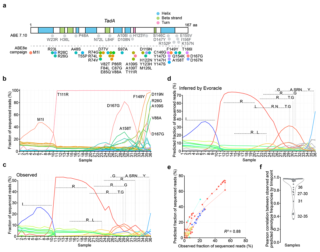
a, The TadA gene (501 nt) annotated with secondary structure regions and non-synonymous mutations in ABE7.10 (14 mutations) and mutations that arose during ABE8 PANCE (34 mutations). Colors represent amino acid mutations. b, Observed frequencies of 34 mutations. Colors match those in Fig. 3a. c, Observed frequencies of full-length genotypes. Samples 1-20 are low stringency PANCE, samples 21-29 are high stringency PANCE, and samples 30-36 are PACE. Colors represent full-length genotypes. d, Inferred full-length genotype trajectories. Samples 1-20 are low stringency PANCE, samples 21-29 are high stringency PANCE, and samples 30-36 are PACE. Samples are in chronological order. PANCE samples were collected every 24 h and PACE samples were collected every 12 h. Colors match those in Fig. 3c. e, Consistency between observed and predicted full-length genotype frequencies. Genotypes are colored in the same manner as Fig. 3c, and lines connect genotypes at neighboring timepoints. f, Consistency between observed and predicted full-length genotype frequencies by timepoint with kernel density estimate.

From the 501-nt reads, we generated synthetic 100-nt segments by sequentially tiled in silico truncation (Online Methods). Evoracle inferred genotype frequency trajectories that closely matched ground-truth trajectories (Fig. 3C–D), achieving R² = 0.88 between predicted and observed full-length genotype frequencies across timepoints (Fig. 3E–F). Inferred fitnesses were also consistent with fitness calculated from full-length sequencing reads (R = 0.80). The model performed strongly in the PANCE stages of the campaign with both low and high selection stringencies (timepoints 1–29) but struggled more in the PACE stage when the lagoon was a more diverse mixture of low frequency genotypes reminiscent of clonal interference⁴² (timepoints 30–36).

While the model performed best under selective sweep conditions in which one or two genotypes dominated the population, the model was not limited to recovering only high frequency genotypes: we also observed accurate reconstruction of time-series frequencies of full-length genotypes such as the double mutant T111R+M126L that never rose above 10% frequency (Fig. 3C–D). On two other replicate directed evolution campaigns, Evoracle performed similarly (R² = 0.85–0.87; Extended Data Fig. 4). The model’s weakest performance occurred at timepoint 32 (after 25 PANCE passages and 36 h of PACE), where it failed to reconstruct an unusual second peak for single mutant T111R. Evoracle can accurately reconstruct full-length genotype trajectories and fitness for evolving genes from both non-continuous and continuous directed evolution platforms.

Effect of read length on reconstruction

We evaluated the impact of reducing read length on Evoracle’s reconstructions. From full-length Cry1Ac and TadA reads, we generated datasets by aligning reads to the reference sequence, then progressively truncating these reads in silico to the limit of 3-nt “post-alignment reads” with loss of linkage between adjacent amino acids. In this scenario, the input data are amino acid frequencies at each timepoint, but no knowledge of mutation co-occurrence frequencies (Fig. 1C, 3B). While Evoracle reconstructed full-length genotype frequencies more accurately with longer read lengths, it performed surprisingly well even with a 3-nt post-alignment read length with a median R² of 0.90 for Cry1Ac evolution and 0.83 for TadA evolution (Fig. 4A–D) across 50 replicates with random parameter initializations (Online Methods). Fitness inferred from reads with complete loss of physical linkage maintained good consistency with ground-truth fitness (R² = 0.67 for Cry1Ac and 0.69 for TadA, Extended Data Fig. 5). These results indicate that Evoracle is robust to shorter read lengths, loss of linkage in reads, and random parameter initializations. Evoracle’s compatibility with very short read lengths suggests its potential to process data from chip array-based DNA sequencing by hybridization technologies, which allow simultaneous DNA sequencing in a very high-throughput manner^43,44.

Fig. 4 |. Robustness to shorter read lengths.

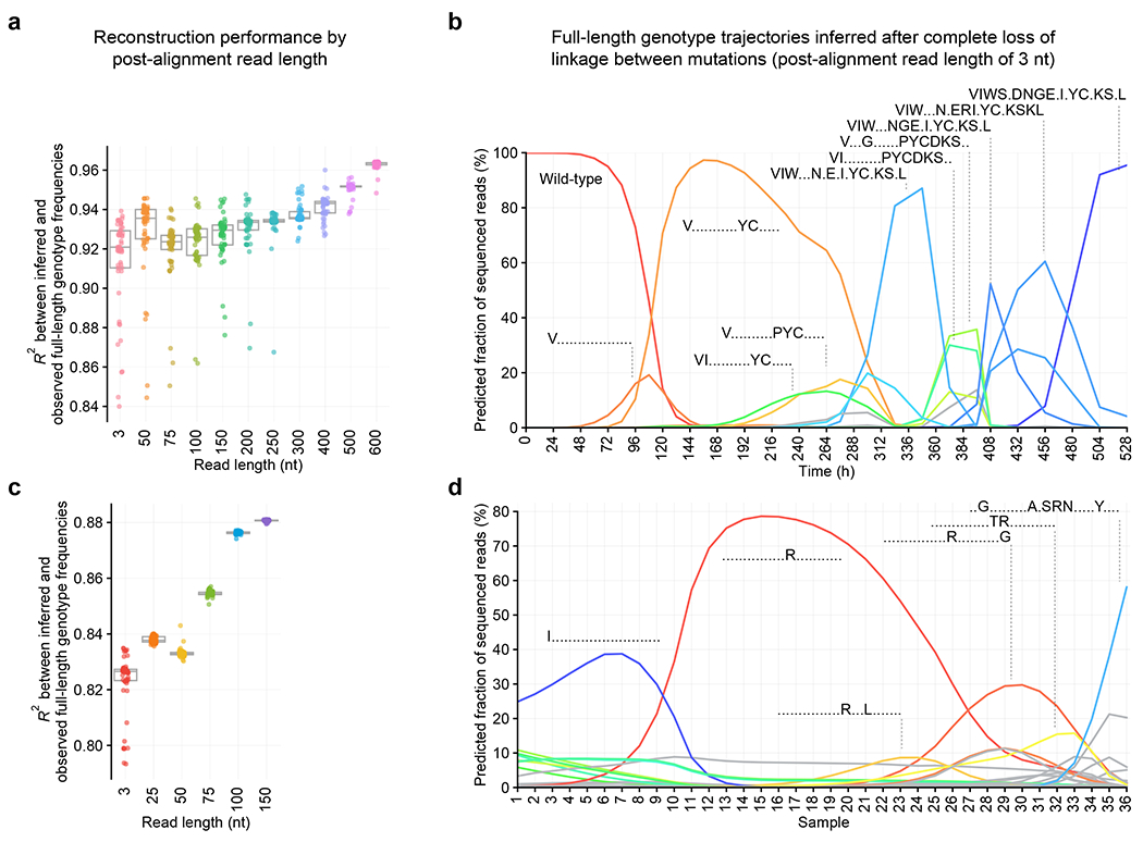
a, Consistency between inferred and observed full-length genotype frequencies by read length for Cry1Ac. Box plot depicts median and interquartile range. N = 50 replicates from random initializations. Colors represent read length. b, Inferred full-length genotype frequencies from reads with a post-alignment length of 3 nt, simulating pooled Sanger sequencing with Surveyor deconvolution, for Cry1Ac. In pooled Sanger sequencing, a mixed trace is aligned to a reference sequence, but co-occurrence frequencies of nucleotides at distinct positions cannot be measured. With a post-alignment length of 3 nt, co-occurrence frequencies of amino acids at distinct positions cannot be measured. Colors represent full-length genotypes and match those in Fig. 1d. c, Consistency between inferred and observed full-length genotype frequencies by read length for TadA. The box plot depicts median and interquartile range. N = 50 replicates from random initializations. Colors represent read length. d, Inferred full-length genotype frequencies from 3-nt post-alignment reads for TadA. Colors represent full-length genotypes and match those in Fig. 3c.

Robustness to DNA sequencing errors

We evaluated Evoracle’s robustness to increased noise in the form of DNA sequencing errors. We designed a synthetic noise procedure to inject noise into data with a tunable noise level (standard deviation, s.d.) (Online Methods). We evaluated Evoracle’s reconstructions on Cry1Ac and TadA data with complete loss of linkage and synthetic noise with s.d. ranging from 0% to 25% across 50 replicates. Relative to 0% noise s.d. (mean R² = 0.90, IQR = 0.88–0.93), Evoracle maintained remarkably strong performance on Cry1Ac data with 5% noise s.d. (mean R² = 0.86, IQR = 0.84–0.87) and even with 8% noise s.d. (mean R² = 0.76, IQR = 0.73–0.81; Fig. 5A–C). Compared to TadA data with no noise (R² = 0.82, IQR = 0.82–0.83), Evoracle also maintained remarkably strong performance with 5% noise s.d. (mean R² = 0.76, IQR = 0.74–0.77) with deterioration at 8% noise s.d. and above (Fig. 5D–F). Fitness inferred with 5% noise s.d. from reads with complete loss of linkage also maintained robust performance (R² = 0.52 for Cry1Ac and R² = 0.42 for TadA). Evoracle also maintained robust performance to shallower read depths (Extended Data Fig. 6). Together, these findings suggest that Evoracle is robust to noise levels as high as 5% s.d.

Fig. 5 |. Robustness to measurement noise.

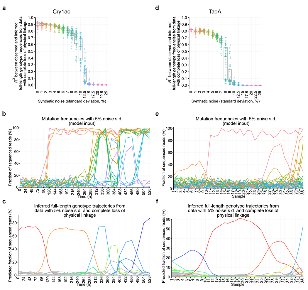
a, Consistency between inferred and observed full-length genotype frequencies with 1-nt reads and varying measurement noise for Cry1Ac. Box plot depicts median and interquartile range. N = 50 replicates with independent noise and random initializations. Colors represent synthetic noise levels. b, Observed positional mutation frequencies for Cry1Ac with 5% measurement noise. Colors represent amino acid mutations and match those in Fig. 1b. c, Inferred full-length genotype trajectories from 1-nt reads with 5% measurement noise for Cry1Ac. Colors represent full-length genotypes and match those in Fig. 1d. d, Consistency between inferred and observed full-length genotype frequencies with 1-nt reads and varying measurement noise for TadA. Box plot depicts median and interquartile range. N = 50 replicates with independent noise and random initializations. Colors represent synthetic noise levels. e, Observed positional mutation frequencies for TadA with 5% measurement noise. Colors represent amino acid mutations and match those in Fig. 3a. f, Inferred full-length genotype trajectories from 1-nt reads with 5% measurement noise for TadA. Colors represent full-length genotypes and match those in Fig. 3c.

Pooled Sanger sequencing of a mixture of variants yields population sequencing traces, which can be analyzed using Surveyor³⁸, EditR³⁹, or other deconvolution methods to estimate single-nucleotide mutation frequencies along a reference sequence with complete loss of linkage between adjacent nucleotides. Surveyor’s noise has been characterized as roughly binomial with a standard deviation of 3% compared to mutation frequencies measured by Illumina methods^38,39. In a previous section, we demonstrated that Evoracle accurately inferred fitness rankings from pooled Sanger sequencing with Surveyor³⁸ deconvolution of OrthoRep directed evolution data of PfDHFR (P = 0.04, Extended Data Fig. 3). Taken together with our synthetic noise results, Evoracle’s reconstructions can be accurate using pooled Sanger sequencing and Surveyor deconvolution, which is generally more accessible and cost-effective than NGS, and can cost as little as ~$10/timepoint (Supplementary Table 1, Supplementary Note 4)^6,17,38,39.

Comparison to related methods

While many methods have been developed for haplotype reconstruction^{20,26,28,45–47}, most require extensive overlaps between reads⁴⁵, or additional input such as long-read⁴⁷ or gene expression data⁴⁶. Overlap-free methods using only short-read data with incomplete linkage can be categorized into model-free and model-based methods. A representative model-free method^28,48 is bacterial haplotype reconstruction (BHap)²⁸, which clusters disconnected linkage groups by frequency to reconstruct haplotypes. However, model-free methods face identifiability problems and have poor guarantees on performance, as without additional information, these methods cannot reconstruct a mixture of haplotypes present at equal frequency. Model-based methods can leverage time-series information, and include Evoracle and the single-segment multi-locus model (SGML)^26,27 which infers genotype frequencies and fitness under the same model of natural selection as Evoracle. SGML considers a restricted mutation model that diffuses genotype frequencies into their single mutants each timestep, while Evoracle introduces novel methodology to perform inference with a more flexible mutation model that induces an intractable likelihood. We refer readers to Supplementary Note 4 for a detailed methods comparison of Evoracle to BHap and SGML.

Notably, BHap and SGML have not been previously evaluated using real full-gene sequencing data. We evaluated each method using the ground truth full-gene sequencing data from the Cry1Ac and TadA datasets, and considered various types of input data, including short reads with 100-nt of linkage (Illumina sequencing data) and data with complete loss of linkage between mutations and 5% noise (simulating pooled Sanger sequencing data).

Evoracle performed substantially better (R² = 0.76–0.94) than BHap (R² = 0.01–0.31) and SGML (R² = 0.00–0.01) across six evaluation tasks (Fig. 6A). BHap assumes that no genotypes have similar frequency, and assumes that mutations around the lowest observed frequency belong to the same genotype. We speculate that BHap’s performance performs poorly when a diverse mixture of genotypes occur at low frequency, which is typical of directed evolution. While SGML successfully reconstructed a high-fitness Cry1Ac genotype that swept the population near the final timepoint, SGML tends to find solutions with a single slow sweep (Extended Data Fig. 7). SGML struggles with reconstructing multiple selective sweeps observed in our directed evolution datasets due to its restrictive model of evolution. When populations evolve under high selection stringency and high mutation rates, novel high-fitness genotypes can arise that differ by many mutations from common genotypes via many intermediate sequences that have low or undetectable frequencies, which can be difficult for SGML’s explicit mutation model to reconstruct. In contrast, a key property of Evoracle is that it flexibly allows any genotype to enter the population at any timepoint, improving its performance on evolutionary data where large jumps in sequence space can occur. These results demonstrate that Evoracle offers a substantial improvement over prior methods.

Fig. 6 |. Model-guided fitness optimization.

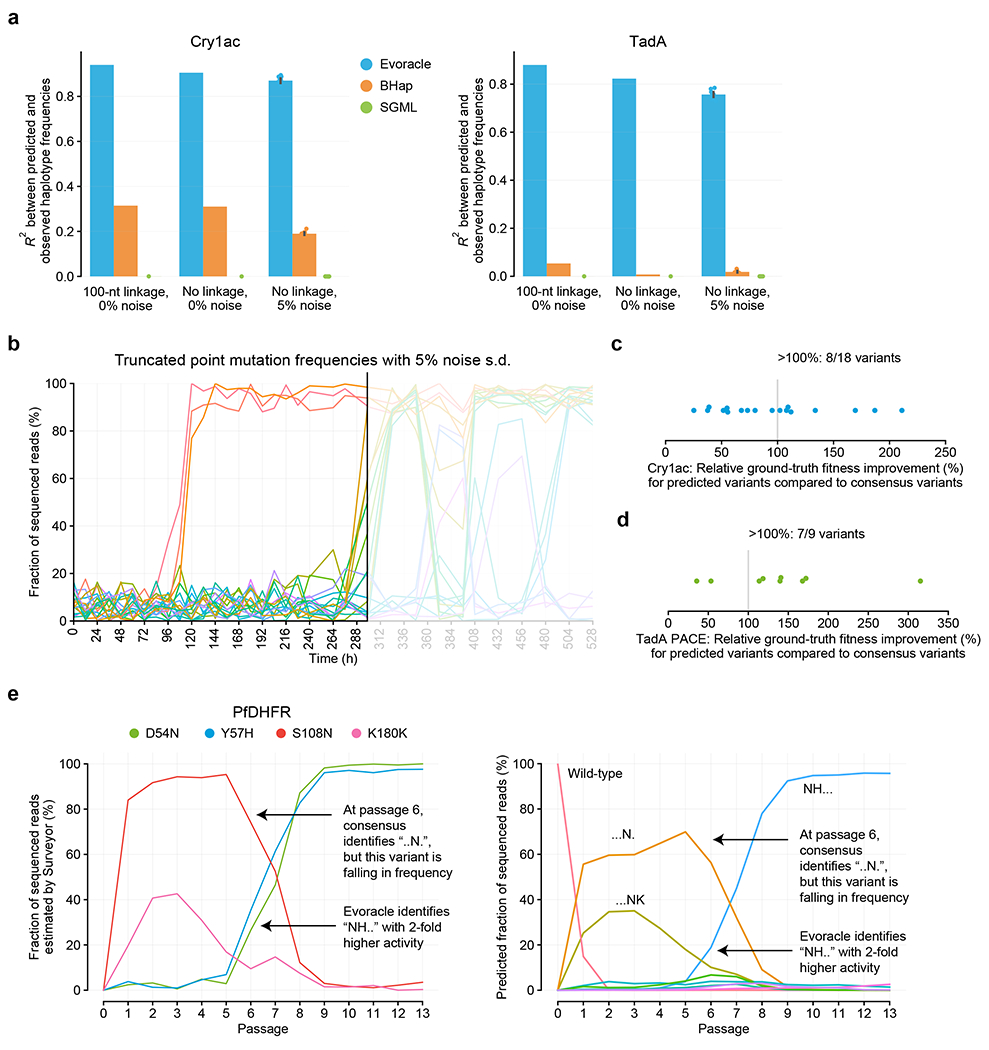
a, Performance comparison of Evoracle to related methods on the Cry1ac and TadA datasets. N=1 experiment for noiseless conditions, and N=10 experiments for noise conditions. Error bars indicate standard error of the mean across replicates with independent noise. b, Example of truncated data analysis. Colors represent amino acid mutations and match those in Fig. 1b. c, Cry1Ac truncated datasets. Ground-truth fitness of unique variants predicted by Evoracle to have higher fitness than the consensus variant. d, TadA truncated datasets at PACE timepoints. Ground-truth fitness of unique variants predicted by Evoracle to have higher fitness than the consensus variant. Values in (c) and (d) are normalized such that the consensus variant ground-truth fitness is 1. e, Mutation trajectories for PfDHFR evolution campaign 2 in OrthoRep, annotated with variants identified by Evoracle and the consensus approach. Left: colors represent amino acid mutations and match those in Fig. 2b. Right: colors represent full-length genotypes and match those in Fig. 2e.

One alternative to using Evoracle with pooled Sanger sequencing data is using data from Sanger sequencing of many clones. In our analysis, clonal Sanger sequencing data requires 10x more resources (~$100/timepoint) to match Evoracle’s performance with a single pooled Sanger sequencing sample (Extended Data Fig. 7, Supplementary Note 4).

Identification of gene variants with high fitness

We compared Evoracle’s ability to propose variants with high fitness to the commonly used approach of proposing variants comprising consensus mutations with >50% frequency at the last timepoint of directed evolution campaigns^{3,5,6,11,12,29–31}. For gene-length biomolecules, using consensus mutations to nominate high-fitness genotypes can result in incomplete sets of epistatic interactions, or suboptimal mutation combinations by mixing variants. Furthermore, proposing genotypes using only the last timepoint ignores time-course information: for example, variants with high but decreasing frequency have lower fitness than variants with low but increasing frequency. Motivated by Evoracle’s fitness inference performance (R² = 0.64–0.71; Extended Data Fig. 5), we hypothesized that Evoracle could propose genotypes with higher fitness than the consensus mutation approach. We evaluated Evoracle’s performance on data with complete loss of linkage and 5% noise (simulating a pooled Sanger sequencing strategy) truncated at every timepoint (Fig. 6B). Proposed variants were evaluated using ground-truth fitness (relative genotype replication rates) calculated using held-out full-length genotype frequencies.

On the Cry1Ac dataset truncated at 32 different timepoints, Evoracle predicted a total of 18 gene variants with higher fitness than the consensus variant with eight hits for an accuracy of 44% (Fig. 6C). The improved Cry1Ac variants had an average of 142% higher fitness and up to 211% higher fitness than the consensus variants at the same timepoints (Fig. 6C). Evoracle also performed well on TadA data, with a hit rate of 32/44 in the PANCE truncated datasets, and 7/9 in the PACE regime (Fig. 6D) for an accuracy of 76%. The improved TadA variants had an average of 151% higher fitness and up to 315% higher fitness than the consensus variants.

In the OrthoRep campaign 2, Evoracle identified “NH..” as a high-fitness variant two passages (>48 h) earlier and “.HN.” three passages (>72 h) earlier than the consensus method. At passage 6, the consensus variant was “..N.” while Evoracle identified “NH..” which had two-fold higher MIC of pyrimethamine⁶ (Fig. 6E). A particular advantage of Evoracle over the consensus mutation approach is the ability to identify high-fitness ‘rising star’ variants even when their frequency is low. In one PfDHFR campaign, Evoracle was able to identify the variant “NH..” with two-fold higher pyrimethamine resistance more than 48 h before the consensus method, when the mutations D54N and Y57H were at 25% to 35% frequency (Fig. 6E). In timepoints 192–276 h in the Cry1Ac campaign (Fig. 1D), the consensus method called the variant A-76V, D387Y, S404C with high but decreasing frequency, while Evoracle was able to identify variants including M-73I and S363P with low but rising frequencies of 10% to 15% which had higher fitness. Overall, these comparisons across three datasets demonstrate that Evoracle can identify variants with higher fitness than those identified with the common consensus approach.

Identifying variants with strong phenotypic activity

We investigated Evoracle’s ability to propose variants with higher biochemical activity measured by phenotypic assays. Thus far, we have evaluated Evoracle’s variant prioritization based on fitness (defined as relative genotype replication rates) calculated from ground-truth genotype frequencies. However, fitness under designed selections can have an imperfect relationship to the end-goal biochemical activity - for instance, mutations that reduce protein stability can propagate effectively in directed evolution but reduce activity in validation assays^3,49. Following PACE³, seven anti-insecticidal Cry1Ac variants were designed by humans based on consensus mutations for synthesis. Among these variants, Evoracle inferred that the genotype “WS.DNGE.I.YC.KS.L” had the highest fitness from data with complete loss of physical linkage and 5% noise, and this variant indeed proved to have the highest larval mortality across toxin doses ranging from 10⁻¹ to 10² ppm³, with up to 10-fold higher larval mortality rates than other tested variants. Across three OrthoRep campaigns and using only pooled Sanger sequencing data, Evoracle correctly identified the PfDHFR variants with the best log₁₀ MIC of pyrimethamine [M] among tested variants (Extended Data Fig. 3), with up to 2-fold improvement over other variants. Together, these observations suggest that Evoracle can prioritize variants with high biochemical activity.

Discussion

Integrating machine learning and directed evolution to propose genotypes with optimized fitness has had longstanding interest in the molecular life sciences^50–55. Standard supervised machine learning approaches, however, require full-length genotypes with activity annotations, which have not been previously accessible at scale for gene-length biomolecules. By reconstructing full-length genotypes with fitness annotations, Evoracle can generate training data from short-read sequencing data on gene-length biomolecules and expand the intersection between machine learning and directed evolution.

Evoracle (https://github.com/maxwshen/evoracle) is a machine learning method that leverages covariation in point mutation frequencies over time to accurately reconstruct fitness and frequencies of full-length genotypes from directed evolution timepoints, even with very short DNA sequencing read lengths and substantial measurement noise such as sequencing errors. We validated Evoracle on data from three campaigns across three directed evolution platforms: PACE, PANCE, and OrthoRep, and reported a new dataset with full-gene sequencing and short read data in 99 samples spanning 37 timepoints from a directed evolution campaign on TadA²⁹. We demonstrate that Evoracle substantially outperforms two related overlap-free genotype reconstruction methods. By reconstructing full-length genotypes, Evoracle can help reveal the molecular basis of activity improvements. Epistatic interactions between mutations at distant residues can be deciphered by analyzing genotype fitness. Importantly, we showed that Evoracle can propose genotypes with higher fitness and activity compared to typical experimental workflows that focus on consensus mutations, including ‘rising star’ genotypes with low frequency but higher fitness than the consensus variant. Finally, we demonstrated that all these aspects of Evoracle are compatible with pooled Sanger sequencing with Surveyor deconvolution, which is substantially more accessible and cost-effective than alternatives such as long-read NGS.

Evoracle advances overlap-free genotype reconstruction methodology and could extend beyond directed evolution of gene-length biomolecules. Since Evoracle requires no linkage between mutations, in principle Evoracle may be able to recover fitness interactions between nucleotides in different genes, or even in the genomes of distinct species. Although Evoracle was designed to study evolution experiments with high selection stringency, mutation rates, and large population sizes where timepoint samples can be easily acquired, Evoracle might also be applied to cancer evolution or other natural evolutionary processes.

Methods

High-throughput sequencing

Phage samples from individual time points during the ABE8e evolution campaign were used for high-throughput sequencing. 1 uL of each sample was used for PCR with primers KZ1532 (5’-ATAAACTGATACAATTAAAGGCTCC-3’) and KZ1533 (5’-GGTGTTTCGCTACCGGAAGAACCAC-3’) to yield PCR products of 602 base pairs in length. PCR activation was done at 95 °C for 10 min to ensure phage lysis, followed by 30 cycles of 30 second extensions. After each sample was confirmed by agarose gel, a second round of PCR for 10 additional cycles was performed to barcode each sample individually. All samples were then pooled at comparable amounts and sequenced using an Illumina MiSeq v2 600-cycle kit.

Cry1Ac data processing

The Cry1Ac dataset is from a PACE directed evolution campaign on the gene Cry1Ac³. PacBio sequencing reads, Illumina sequencing reads, and the Cry1Ac reference sequence were obtained from Badran et al.³ and NCBI Sequence Read Archive accession number PRJNA293870. Following their methods, PacBio data were aligned to the reference sequence using blasr version 5.3.3 with default parameters. Reads with fewer than 2,000 matches (out of a reference sequence length of 8,326 nucleotides) were discarded. Non-synonymous amino acid mutations among a list of 19 high-confidence mutations derived from Badran et al. were tabulated; these mutations were A-76V, M-73I, C15W, F68S, R198G, G286D, T304N, E332G, A344E, Q347R, T361I, S363P, D384Y, S404C, N417D, E461K, N463S, E515K, and S582L. Full-length genotype frequencies were tabulated after discarding reads that contained a deletion at any high-confidence mutation position. Following the methods of following Badran et al., full-length genotypes that did occur at >1% frequency at any timepoint were discarded; at this point, approximate PacBio read depth was on the order of 10², so this step corresponded to filtering genotypes with no more than a handful of reads at all timepoints.

Paired end 2x150 Illumina reads were aligned to the reference sequence using bowtie2 version 2.3.5.1 using default settings. Non-synonymous amino acid mutations were reduced to the previously described list of 19 high-confidence mutations from the study. The reference sequence was split into 100-nt segments and mutation combination frequencies were tabulated using all reads spanning each segment.

TadA data collection and processing

The TadA dataset is from a PACE and PANCE directed evolution campaign on the E. coli TadA gene (167 amino acids), which encodes a tRNA adenosine deaminase converts adenine to inosine⁴⁰, which is used in adenine base editors (ABEs)⁴¹. Directed evolution occurred over more than 444 h. Due to the short length of TadA (501 nt), 600-nt Illumina sequencing reads were used to read full-length genotypes. The dataset contains 99 samples collected from parallel evolutions across 37 unique timepoints at an average depth of 110,461 reads per timepoint.

We obtained 2x300 bp Illumina sequencing data for 99 samples, comprising 20 samples for each of two low-stringency phage-assisted non-continuous evolutions (PANCEs) (samples 1-20 and 21-40), 9-10 samples for four high-stringency PANCEs (samples 41-50, 51-60, 61-69, and 70-78), and 7 samples for three phage-assisted continuous evolutions (PACEs) (samples 79-85, 86-92, and 93-99). All consecutive samples were collected 24 h apart (within the same regime) or more (across regimes) except for one consecutive pair collected 12 h apart. Pandaseq 2.7 was used to merge overlapping paired-end Illumina sequencing reads with default settings, and bowtie2 version 2.3.5.1 was used to align merged reads to the ABE 7.10 reference sequence with default settings. Non-synonymous mutations that occurred at greater than 5% frequency in at least one sample were retained as ‘major’ mutations; these 34 mutations were verified to include all significant mutations described by Richter et al.²⁹ and consisted of M1I, R23L, R26C, R26G, A48S, T55P, R74G, R74L, R74V, D77V, V82T, F84L, E85Q, P86R, C87G, V88A, S97A, A109S, A109T, T111R, D119N, H122N, Y123H, M126L, C146G, Y147D, Y147H, Y147S, F149Y, Q154K, A158T, T166I, D167G, and D167N. Full-length genotype frequencies were aggregated by summation to reduce them into the set of major mutations. At this point, full-length genotypes occurring with 5 or fewer reads were filtered from each sample. Relevant sequences are provided in Supplementary Sequences.

Following the relationship between the PANCE and PACE regimes in the study²⁹, whereby each low-stringency PANCE was used to seed two high-stringency PANCEs, and all four high-stringency PANCEs were combined to seed each PACE experiment, we combined the two low-stringency PANCE regimes by using a 1:1 mixture of full-length genotype frequencies and re-normalizing. We manually aligned samples to maximize consistency between the four high-stringency PANCEs as some regimes had 9 samples and other regimes had 10 samples and combined their data by a uniform mixture. This yielded full-length genotype trajectories across 20 low-stringency PANCE timepoints, 9 high-stringency PANCE timepoints, and 7 PACE timepoints for a total of 36 timepoints.

Supplementary Sequences

Amino acid sequence of TadA in ABE 7.10

MSEVEFSHEYWMRHALTLAKRARDEREVPVGAVLVLNNRVIGEGWNRAIGLHDPTAHAEIMALRQGGLVMQNYRLIDATLYVTFEPCVMCAGAMIHSRIGRVVFGIRNAKTGAAGSLMDVLHYPGMNHRVEITEGILADECAALLCYFFRMPRQVFNAQKKAQSSTD

DNA reference sequence for TadA and surrounding context

TCTTATAAACTGATACAATTAAAGGCTCCTTTTGGAGCCTTTTTTTTTGGAGTAAGGAGGAAAAATGTCAGAAGTAGAGTTTTCACACGAGTACTGGATGAGACACGCATTGACTCTCGCAAAGCGTGCTCGAGATGAACGCGAGGTGCCCGTGGGAGCAGTACTCGTGCTCAACAATCGCGTAATCGGCGAAGGTTGGAATCGTGCAATCGGACTCCACGACCCCACTGCACATGCGGAAATCATGGCCCTTCGACAGGGCGGGCTTGTGATGCAGAATTATCGACTTATCGATGCGACGCTGTACGTCACGTTTGAACCTTGCGTAATGTGCGCGGGAGCTATGATTCACTCCCGCATTGGACGAGTTGTATTCGGTGTTCGCAACGCCAAGACGGGTGCCGCAGGTTCACTGATGGACGTGCTGCATTACCCAGGCATGAACCACCGGGTAGAAATCACAGAAGGCATATTGGCGGACGAATGTGCGGCGCTGTTGTGTTACTTTTTTCGCATGCCCAGGCAGGTCTTTAACGCCCAGAAAAAAGCACAATCCTCTACTGACTCTGGTGGTTCTTCTGGTGGTTCTTCCGGTAGCGAAACACC

PfDHFR data processing

The PfDHFR dataset is from an OrthoRep directed evolution campaign that evolved antimalarial drug resistance to pyrimethamine in Plasmodium falciparum malarial dihydrofolate reductases (PfDHFRs)⁶. Measurements were taken using pooled Sanger sequencing and Surveyor.

Position-wise mutation frequencies were calculated from vectorized figures obtained from the OrthoRep study⁶ using rulers in Adobe Illustrator. Specifically, figures 3C, 3D and S5A were used. Distances can be measured in vector graphics to arbitrary precision; we used a measurement resolution of 0.001 points and calculated the y-value of each point compared to the y-axis. A range of 100% frequency in the y-axis corresponded to 100.863 points, so our resolution of 0.001 points translated to a frequency resolution of 0.001%.

Fitness values were obtained from Fig. 4. Fitness ranges were provided as text. Fitness midpoints (out of three replicates) were depicted as the color of each box and converted to a number using the color bar in each subfigure. The color bar was converted to a pixelized format and the nearest color pixel to a box’s color was used to estimate the fitness value to a resolution of 0.1.

Inference problem definition

We consider a stochastic non-linear dynamical system that describes directed evolution. The latent state at time t is a vector of genotype frequencies x_t, which undergo the following state transition process each timestep: first, genotype frequencies are updated according to a standard model of asexual fitness-based natural selection^26,32 as $\frac{\mathit{w}}{{\mathit{w}}^{\mathit{T}}{\mathit{x}}_{\mathit{t}}}\odot {\mathit{x}}_{\mathit{t}}$ where w is a non-negative fitness vector, then mutation introduces a genotype i to the population at time t with frequency s[i] if z[i] = t for each i indexing the G genotypes, where z[i] ≠ t if x_t[i] > 0. These two steps can be expressed in a single equation as $\mathit{E}\left[{\mathit{x}}_{\mathit{t}+1}\right]=\left(1-{\sum }_i{\mathit{p}}_{\mathit{t}}\right)\left(\frac{\mathit{w}}{{\mathit{w}}^{\mathit{T}}{\mathit{x}}_{\mathit{t}}}\right)\odot {\mathit{x}}_{\mathit{t}}+{\mathit{p}}_{\mathit{t}}$ where p_t is a vector whose i-th element is s[i] if z[i] = t otherwise 0, with initial genotype frequencies x_t=0 = p₀.

We observe data at T timepoints through a lossy stochastic observation process E[y_t] = Bx_t, where B is a binary matrix that is rank deficient because the dimension of y_t is smaller than x_t. This measurement process is a generalized description of the process of performing short-read sequencing, then computing the fraction of the population that contains a mutation at some position, for many positions and mutations of interest.

We assume that noise models for the state transition and observation process are known and finite (for example, binomial or beta-binomial observational noise), but we do not focus on noise models since Evoracle is a likelihood-free inference method.

The inference task is: Given y₁, y₂, …, y_T, infer the parameters (w, s, z) and the unobserved genotype frequency states x₁, x₂, …, x_T. This inference task is challenging due to the high dimensionality of the parameters (three per genotype with hundreds of relevant genotypes), the large discrete space of z, and the intractability of computing likelihoods in models that attempt to infer the parameters of a distribution governing z. We discuss related work and alternative inference approaches in the results.

Briefly, Evoracle is a simple likelihood-free inference algorithm supporting efficient gradient-based optimization with faster asymptotic time complexity than conventional expectation maximization approaches. Evoracle bypasses the challenging task of inferring s, z by directly inferring x₁, x₂, …, x_T under the constraints: 1) each genotype enters the population at an arbitrary inferred frequency at most once, 2) frequencies of present genotypes should be consistent with fitness-based natural selection, and 3) absent genotypes have zero frequency. We satisfy these constraints by distinguishing present and absent genotypes using a low positive threshold ϵ, renormalizing present frequencies, and enforcing a gradient-matching regularizer on present genotypes to ensure fidelity to the natural selection process. These steps explicitly handle all constraints except ensuring that genotypes enter the population at most once, which is handled implicitly by encouraging fidelity to the natural selection process.

Evoracle

Here, we describe algorithms for Evoracle and the forward pass computation of our differentiable loss function. We discuss theoretical properties of Evoracle in Supplementary Note 1.

Algorithm 1.

Evoracle.

Input:
-	Observations y1, y2, …, yT
-	Non-negative hyperparameters α, β
-	Hyperparameters for the genotype proposal method
Output:
-	Inferred genotype frequencies ${\widehat{\mathit{x}}}_1,{\widehat{\mathit{x}}}_2,\dots ,{\widehat{\mathit{x}}}_{\mathit{T}}$
-	Inferred parameters ($\widehat{\mathit{w}},\widehat{\mathit{s}},\widehat{\mathit{z}}$)
Steps
1.	Propose genotypes that could exist in the population
Add single mutants
	Add genotypes with multiple mutations that rise or fall together in any consecutive timepoint
G = number of genotypes proposed
2.	Initialize parameters and hyperparameters
	Initialize non-negative ϵ such that Gϵ << 1
	Initialize ${\widehat{\mathit{x}}}_1,{\widehat{\mathit{x}}}_2,\dots ,{\widehat{\mathit{x}}}_{\mathit{T}}$ such that all entries are greater than ϵ
	Initialize $\widehat{\mathit{w}}$
3.	Perform inference by optimizing loss function with gradient descent
	Until convergence:
	loss = differentiable_loss_function(parameters, hyperparameters)
	Update ${\widehat{\mathit{x}}}_1,{\widehat{\mathit{x}}}_2,\dots ,{\widehat{\mathit{x}}}_{\mathit{T}},\widehat{\mathit{w}}$ using gradient of loss
4.	Recover $\widehat{\mathit{s}}$ and $\widehat{\mathit{z}}$
	$\widehat{\mathit{z}}=\text{A}$ vector of the earliest timepoint where each genotype i has >ϵ frequency in ${\widehat{\mathit{x}}}_1,{\widehat{\mathit{x}}}_2,\dots ,{\widehat{\mathit{x}}}_{\mathit{T}}$ for each i.
	$\widehat{\mathit{s}}=\text{A}$ vector of the frequency of genotype i in ${\widehat{\mathit{x}}}_{\mathit{t}}$ where t = z[i] for each i.
	Return ${\widehat{\mathit{x}}}_1,{\widehat{\mathit{x}}}_2,\dots ,{\widehat{\mathit{x}}}_T$ and $\widehat{\mathit{w}},\widehat{\mathit{s}},\widehat{\mathit{z}}$

We first describe our genotype proposal heuristic, then describe our differentiable loss function. Generally, SNPs or mutations are described by a specific amino acid residue at a particular position. However, combinations of SNPs can be observed by short-read sequencing across multiple nucleotides (and equivalently, amino acids). To represent both cases, we refer to ‘symbols’ occurring at ‘positions’, where a ‘symbol’ can be a single amino acid residue or a combination of amino acid SNPs, and ‘positions’ correspond to the range of amino acids observed in each contiguous and non-overlapping measurement across the reference sequence.

Illingworth et al.²⁶ describes a maximal genotype proposal strategy, which produces an exponentially many (2^N) genotypes for N separately measured mutations. Here, we describe a genotype proposal strategy that scales better by proposing substantially fewer genotypes by focusing on genotypes that are likely to be in the population based on short-read data. In our standard proposal strategy, we first include every single mutant corresponding to a non-reference symbol at a single position and the reference symbol at all other positions. Then, at each consecutive pair of timepoints, combinations of symbols at distinct positions that rise or fall together in absolute frequency greater than “change_threshold” (we used 2.5%), where the symbols’ absolute changes are sufficiently similar (difference < “split_threshold”, set to 5% in our work) are used to form additional full-length genotypes built by using the majority frequency symbol (occurring at greater than “majority_threshold”, set to 50% in our work) at all other non-covarying positions. In situations where no symbol has greater than the majority_threshold frequency at a position, we used the wild-type symbol. Finally, we add the consensus variant at every timepoint.

In our work, we also explored the impact of using a combinatorial proposal approach to evaluate method robustness and sensitivity to mis-specifying or over-specifying full-length genotypes. An exponential number of genotypes were proposed as the Cartesian product of the top 14 positions and symbols ranked by mean frequency across time. In some cases, we keep only a random fraction. We find that Evoracle retains efficient runtime and robust performance when proposing many genotypes.

Algorithm 2.

Differentiable forward pass to calculate loss for a pair of timepoints.

Input:
-	Inferred ${\widehat{\mathit{x}}}_{\mathit{t}},{\widehat{\mathit{x}}}_{\mathit{t}-1}$, w
-	Hyperparameters 0 < ϵ << 1, α > 0, β > 0
Output:
-	Scalar loss. This algorithm is differentiable, which is used to compute a gradient for updating ${\widehat{\mathit{x}}}_{\mathit{t}},{\widehat{\mathit{x}}}_{\mathit{t}-1}$, and w to minimize the loss.
Steps
1.	Calculate present genotypes with threshold ϵ
	$\widehat{{\mathit{z}}_{\mathit{t}}}=[\widehat{{\mathit{x}}_{\mathit{t}}}[\mathit{i}]\text{if}\widehat{{\mathit{x}}_{\mathit{t}}}[\mathit{i}]>\mathbf{ϵ}$ else 0 for i in range(G)]
	${\widehat{z}}_{t-1}=[{\widehat{x}}_{t-1}[i]\mathrm{if}{\widehat{x}}_t[i]>ϵ$ else 0 for i in range(G)]
2.	Normalize frequencies
	$\widehat{{\mathit{z}}_{\mathit{t}}}=\widehat{{\mathit{z}}_{\mathit{t}}}/\text{sum(}\widehat{{\mathit{z}}_{\mathit{t}}}\text{)}$
	${\widehat{\mathit{z}}}_{\mathit{t}-\mathbf{1}}={\widehat{\mathit{z}}}_{\mathit{t}-\mathbf{1}}/\text{sum(}{\widehat{\mathit{z}}}_{\mathit{t}-\mathbf{1}}\text{)}$
3.	Calculate loss terms for time t
	$$L_{data}=D_{KL}(B{\widehat{z}}_t\Vert y_t)$$
	$$L_{fidelity}={\text{D}}_{\mathrm{KL}}\left(\frac{\widehat{w}}{{\widehat{w}}^T{\widehat{z}}_{t-1}}\odot {\widehat{z}}_{t-1}\Vert {\widehat{z}}_t\right)$$
	$$L_{skew}=\sum _i({\widehat{z}}_t[i]-1/G{)}^3$$
	Return Lfidelity + αLdata + βLskew

The state transition process fidelity term compares the fitness-based updated genotype frequencies for genotypes present at t − 1 to the normalized frequency of the same genotypes at time t, because the state transition process specifies that natural selection occurs before new genotypes are introduced at time t.

In practice, our implementation of this algorithm ignores the normalization steps for $\widehat{{\mathit{z}}_{\mathit{t}}}$ and ${\widehat{\mathit{z}}}_{\mathit{t}-1}$, as we assume that Gϵ ≪ 1: the total number of genotypes modeled multiplied by ϵ is small, which means not normalizing incurs a very minor bias. In practice, it is difficult for G to be high due to the limitations of the lossy measurement process, and is often ~100, while we use ϵ = 10⁻⁶ in our work, and in general decreasing ϵ has no impact until machine precision limits are reached. A practical benefit of skipping these normalization steps is that otherwise, inferred genotype frequencies below ϵ no longer participate in any loss term either, and thus will not be updated in future gradient descent updates. For this reason, when using normalization, all genotype frequencies should be initialized above ϵ.

In practice, we introduce ${\widehat{\mathit{z}}}_{\mathit{t}}^{*}=[{\widehat{\mathit{x}}}_{\mathit{t}}[\mathit{i}]\text{if}{\widehat{\mathit{x}}}_{\mathit{t}-1}[\mathit{i}]>\mathbf{ϵ}$ else 0 for i in range(G)], normalize it as ${\widehat{\mathit{z}}}_{\mathit{t}}^{*}={\widehat{\mathit{z}}}_{\mathit{t}}^{*}/\text{sum(}{\widehat{\mathit{z}}}_t^{*}\text{)}$, and use a modified ${\mathrm{D}}_{\mathrm{KL}}\left(\frac{\widehat{\mathit{w}}}{{\widehat{\mathit{w}}}^{\mathit{T}}{\widehat{\mathit{z}}}_{\mathit{t}-1}}\odot {\widehat{\mathit{z}}}_{\mathit{t}-1}\Vert {\widehat{\mathit{z}}}_{\mathit{t}}^{\mathit{*}}\right)$ fidelity term. This sacrifices the implicit regularization that encourages lower L₁-norm on s, but helps avoid instabilities from high KL divergence values which can arise when many new genotypes are introduced at high total frequency at time t. We did not observe these instabilities on our datasets, but prefer this conservative choice in our implementation for our general-use package.

The loss function was implemented in PyTorch⁵⁶ 1.4.0 and optimized using gradient descent. As default settings, we used 1000 optimization epochs, a learning rate of 0.1, weight decay of 1e-5, and a learning rate scheduler that reduced learning rate when the loss plateaued with a patience of 10 epochs, a threshold of 1e-4, and a reduction factor of 0.1. All optimizations performed for this manuscript were done on a single CPU and typically converged within less than one minute to up to five minutes using a 2.80 GHz CPU. We initialize genotype frequencies with a standard normal distribution, and used softmax to obtain normalized frequency distributions. We initialized fitnesses using a normal distribution with mean −1 and standard deviation −0.01, then exponentiated to ensure non-negativity.

Simulating reduced read length

Mutation positions were grouped into reads of a specified length in a naïve manner by starting from the 5’-most mutation (lowest position index) and binning by the simulated read length. We note that simulated read lengths could be repositioned to cover highly variable mutations more optimally, or reduce the number of non-overlapping reads, but we purposefully chose to work with an unoptimized approach to show that such optimization, though helpful in expectation, is not necessary for our model’s performance.

Simulating noise

To simulate a noise at a specified standard deviation s between 0% and 100%, we used a variety of approaches depending on the frequency p of a particular non-overlapping read (potentially containing groups of mutations). We used a binomial model for the noise, since 1) this model describes the noise that occurs when read samples are drawn from a single well-mixed population to investigate model performance with reduced read depth, and 2) a binomial distribution provides a good fit to the empirical distribution of noise produced by pooled Sanger sequencing compared to next-generation sequencing of mutation frequencies^38,39. Other common noise models in the life sciences include beta-binomial and negative binomial (gamma-Poisson mixture), which are usually motivated by fitting models to overdispersed data with higher variance than can be specified under a binomial noise model for an observed mean read count. Here, we do not fit our noise model to data, but directly vary the variance of our simulated noise across a wide range. As a result, there is no additional noise that can be achieved under a beta-binomial or negative binomial model.

We observed that binomial noise would sometimes yield 1) highly discretized noise values (when N is low), and 2) would add less noise than specified when p is near 0 or 1 (that is, the added noise’s standard deviation was less than our specified noise level s). We wanted to avoid highly discretized noise, which would primarily be expected to occur if read depth was extremely shallow, because discretized noise does not accurately represent noise from Surveyor deconvolution. We also wanted to ensure that we never added less noise than specified. Thus, we augmented our binomial noise model to address these two issues.

If p was initially between 0.01 and 0.99, we calculated an effective number of reads n as:

$$n={\left(\sqrt{\frac{p(1-p)}{s}}\right)}^2$$

Then, if n > 20, we sampled a new p ~ binomial(n, p)/n which draws from a distribution with standard deviation s. Otherwise, if n was too small, we avoided extreme discretization by repeatedly sampling a new p ~ Gaussian(p, s) until p was greater than 0 and less than 1.

If p was initially less than 0.01 or greater than 0.99, the above procedure would yield an approximation to a half-Gaussian distribution which has standard deviation smaller than s, which means that less noise is added than desired. Specifically, a Gaussian with variance s² that is truncated in half has variance s²(1 − 2/π) < s². Thus, a Gaussian with

$$std=s{\left(1-\frac{\text{2}}{\text{π}}\right)}^{-1/2}$$

where the scaling factor ≈ 1.659, when truncated in half, yields a half-Gaussian with standard deviation equal to s. To ensure that the specified amount of noise was added at these boundary conditions, we resampled p from a half-Gaussian derived in this manner to ensure its standard deviation was equal to s and not lower.

Calculating fitness from full-length genotype frequencies

To evaluate Evoracle, we compared inferred fitness to ground-truth fitness values w computed from the ground-truth full-length genotype frequencies x₁, x₂, …, x_T for the Cry1ac and TadA datasets. To compute w, we minimized $KL\left(\frac{\mathit{w}}{{\mathit{w}}^{\mathit{T}}{\mathit{x}}_{\mathit{t}}}\odot {\mathit{x}}_{\mathit{t}}\right)$ using gradient descent.

Proposing consensus variants

From an input set of mutation frequencies at given positions at a particular timepoint, we formed the full-length consensus variant by using the amino acid with >50% frequency at each position, or the wild-type amino acid if no mutation surpassed 50% frequency.

Predicting variants with higher fitness than the consensus

From an input matrix of mutation frequencies with complete loss of physical linkage and 5% noise, we used Evoracle to reconstruct full-length genotypes and fitnesses. To compare against a consensus baseline, we formed a consensus variant using mutation frequencies at the final timepoint. To obtain a list of variants predicted by Evoracle to have higher fitness than the consensus, we found all variants with higher predicted fitness than the consensus variant’s predicted fitness. To retain variants with higher confidence predictions, we filtered variants that had less than 5% predicted frequency in the final timepoint (this threshold was motivated by the 5% noise in the data).

To evaluate performance, we used ground-truth fitnesses calculated using held-out full-length genotype data. We calculated the ground-truth fitness of the consensus variant and used the ground-truth fitnesses to evaluate whether each variant predicted by Evoracle to have higher fitness than the consensus actually had higher ground-truth fitness.

We focus on accuracy (true positive rate among predicted positives) and not other binary classification metrics because the class of true positives contains many low-frequency genotypes that are difficult for any method to identify from sequencing data with incomplete linkage.

Non-linear interpolation of full-length genotype frequencies

To investigate the effects of gathering samples at finer time resolution, we interpolated data between two timepoints P_t and P_t+1 of a given dataset of full-length genotype frequencies that are one unit of time apart. Due to measurement limitations, genotypes reported with zero frequency are generally indistinguishable from exceedingly rare genotypes; as such, we replaced zeros that occurred exactly once for a particular full-length genotype in P_t and P_t+1 with a tunable value ε which was set to 1e-6 in this work. P_t and P_t+1 were then renormalized to sum to one. We calculated fitness for all full-length genotypes using P_t and P_t+1 and apply Lemma 4 (Supplementary Note 1) to convert these fitness values to a smaller time unit denoted δ that is less than 1. We then generate interpolated full-length genotype frequencies at time resolution δ for 1/δ total discrete steps between P_t and P_t+1. In practice, this procedure yields frequency trajectories that are smooth piecewise with discontinuities at observed timepoints.

Mutational families

It is common practice in directed evolution experiments to constrain one’s focus to a subset of mutations that are particularly common across the campaign, and to consider only these mutations when designing variants that represent the output of directed evolution for downstream low-throughput characterization or validation. In our work, we used a threshold of 5%. Our analysis follows this practice and refers to combinations of amino acids at these common mutation positions as “full-length genotypes”.

Data Availability

The sequencing data generated during this study are available at the NCBI Sequence Read Archive database at accession code PRJNA625117. Processed data have been deposited under the DOI 10.6084/m9.figshare.12121359.

Code Availability

The code used for data processing and analysis are available at https://github.com/maxwshen/evoracle-dataprocessinganalysis. The Evoracle model is available at https://github.com/maxwshen/evoracle.

Extended Data

Extended Data Fig. 1. Evoracle model properties.

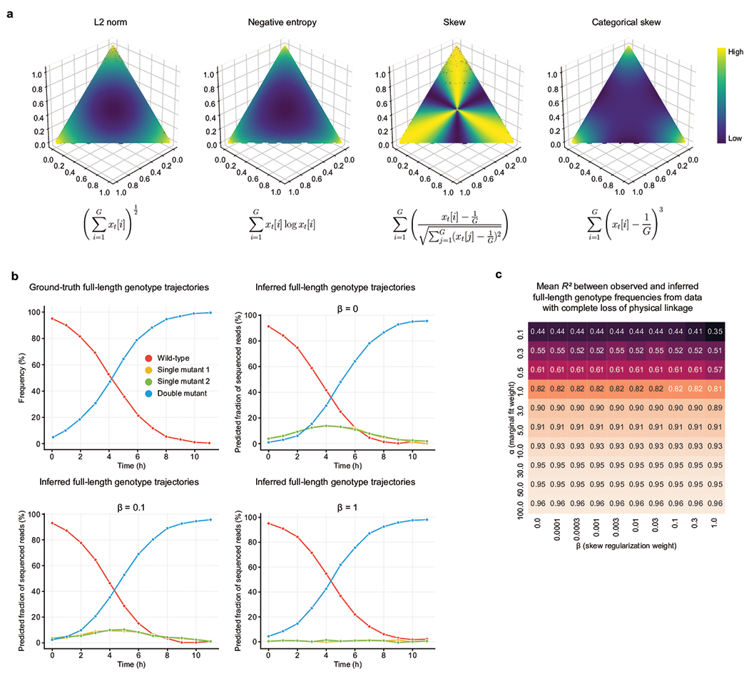
a, Regularization strategies. Comparison of loss incurred by L2 norm, variance, normalized statistical skew, and unnormalized statistical skew (our skew) regularizers for distributions of three variables. b, Synthetic data to demonstrate the utility of the skew regularizer. The top left graph shows a ground-truth simulated population containing only a wild-type genotype and a double mutant. Observed single-mutation frequencies from the ground-truth simulation were used by Evoracle to infer full-length genotype trajectories of the wild-type genotype, both single mutants, and the double mutant. Evoracle was performed with varying values of beta (top right, bottom left, and bottom right). When beta is higher, Evoraclemore correctly infers the ground truth trajectories. Inferred genotype frequencies are plotted with a small jitter to show overlapping lines clearly. c, Robustness to hyperparameters. Performance while varying hyperparameters alpha and beta for Cry1Ac data. Reported statistics summarize performance across ten replicates with random parameter initializations.

Extended Data Fig. 2. Evaluating Evoracle’s genotype proposal strategy.

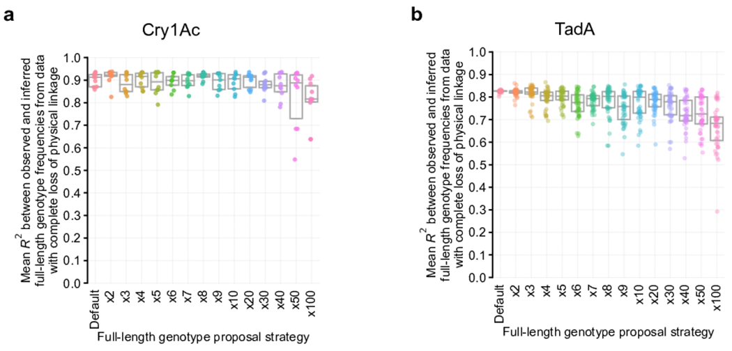
a-b, Sequence proposal strategies. Performance with varying full-length genotype proposal strategies for (a) Cry1Ac data, and (b) TadA data. N = 40 replicates. Box plot depicts median and interquartile range. Default strategy is described in the Online Methods; x2 to x100 represent adding full-length genotypes comprising combinations of mutations to increase the total number of reconstructed full-length genotypes by the stated multiplicative factor of the default number. See Online Methods for more details.

Extended Data Fig. 3. Evolutionary fitness reconstruction from pooled Sanger sequencing of Ortho Repcampaignsa.

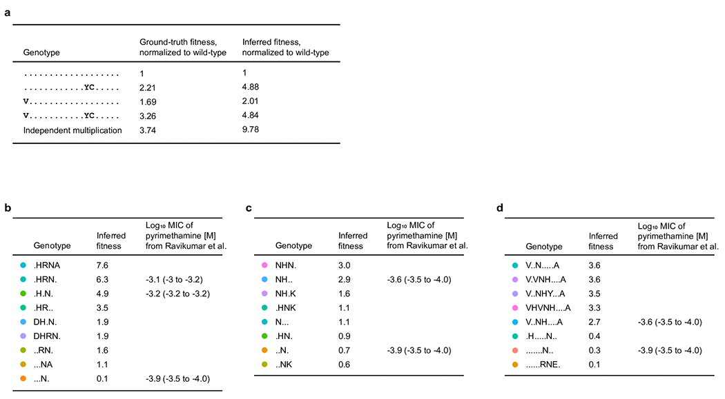
a, Comparison of ground-truth and inferred fitness, indicating a negative epistatic interaction between A76V and D384Y, S404C in Cry1Ac. b-d, Comparison of MIC values and inferred fitness for evolved PfDHFR variants.

Extended Data Fig. 4. Evoracle performance on ABE8e evolution replicates.

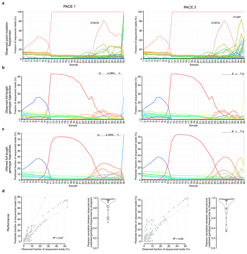
Model evaluation on replicate PACE experiments 1 and 3 of the ABE8e directed evolution campaign. Samples 1-20 are from low-stringency PANCE, samples 21-29 are from high-stringency PANCE, and samples 30-36 are from PACE. a, Observed frequencies of 34 mutations. Colors represent amino acid mutations, using the same coloring scheme as in Fig. 2a–b. b, Observed full-length genotype trajectories. Colors represent full-length genotypes, using the same coloring scheme as in Fig. 2c–d. c, Inferred full-length genotype trajectories. Colors represent full-length genotypes, using the same coloring scheme as in Fig. 2c–d. d, Consistency between observed and predicted full-length genotype frequencies; scatter plot and swarm plot with kernel density estimate.

Extended Data Fig. 5. Evaluation of fitness inference.

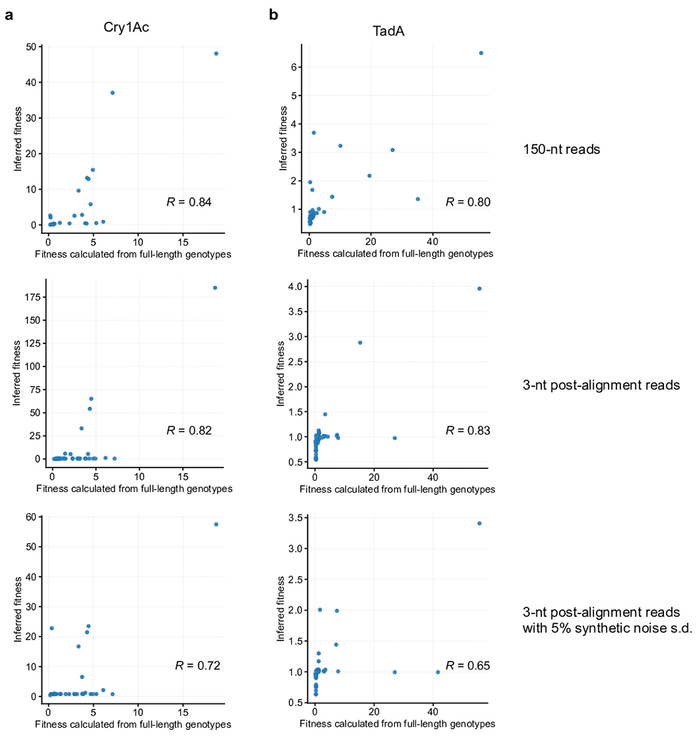
a-b, Comparison of inferred fitness to fitness calculated from full-length reads for (a) Cry1Ac and (b) TadA.

Extended Data Fig. 6. Evoracle performance with varying sequencing read depth.

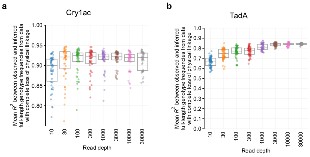
a-b, Full-length genotype reconstruction performance across timepoints with varying simulated read depths using binomial samples for (a) Cry1Ac and (b) TadA. Box plot depicts median and interquartile range. N=50 independent replicates with random seeds.

Extended Data Fig. 7. Comparison to related methods.

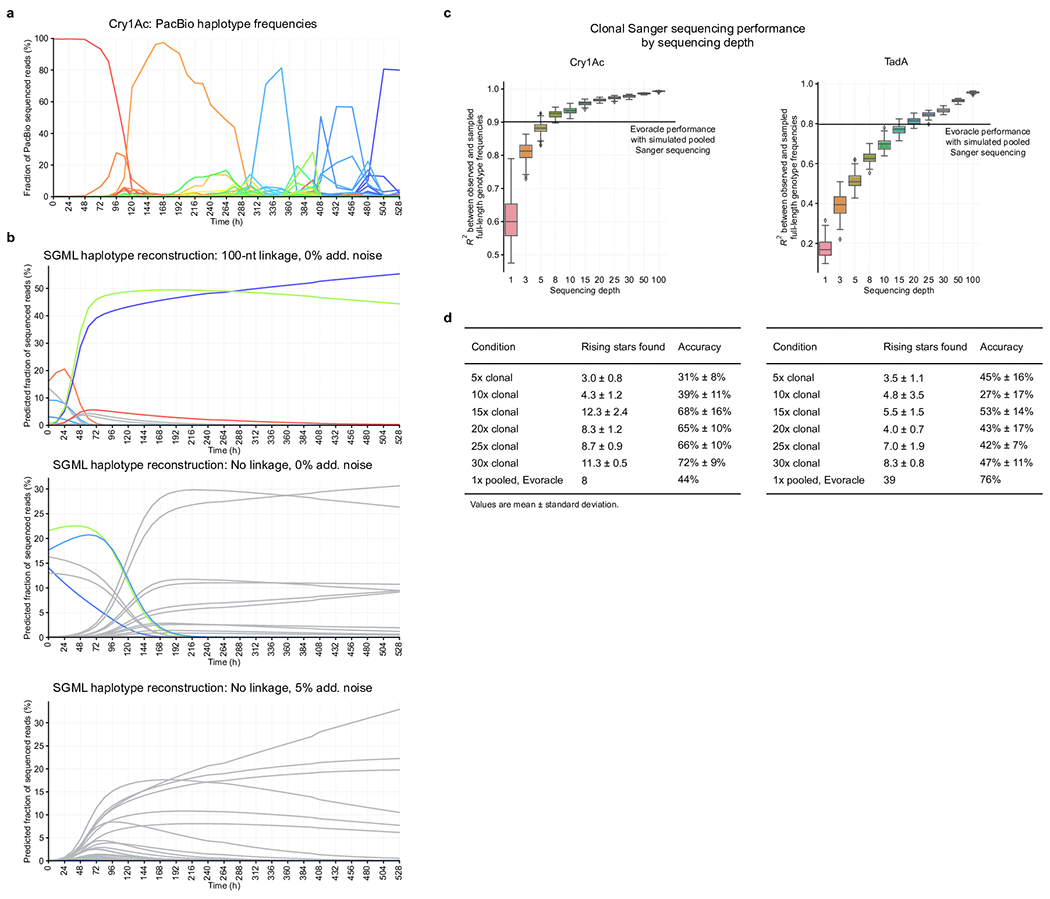
a, Observed Cry1Ac (2,138 nt) genotypes from 34 timepoints (spanning 528 h) of PACE from PacBio long-read sequencing data. Colors represent distinct genotypes. Figure is the same as Fig. 1c and reproduced for convenience. b, Cry1Ac genotype frequencies reconstructed by SGML. Gray lines indicate genotypes that are not present in PacBio data. c, Comparison of performance by clonal Sanger sequencing depth compared to pooled Sanger sequencing. Box plots indicate median and interquartile range, and whiskers indicate extrema. N=50 random seed replicates. d, Comparison of rising star performance by clonal Sanger sequencing depth vs pooled Sanger sequencing on 12 h interpolated Cry1Ac data.

Supplementary Material

Complete SI

Supplementary Table 1, Supplementary Notes 1-4

References

- 1.Packer MS & Liu DR Methods for the directed evolution of proteins. Nat. Rev. Genet 16, 379–394 (2015). [DOI] [PubMed] [Google Scholar]
- 2.Dalkara D et al. In Vivo–Directed Evolution of a New Adeno-Associated Virus for Therapeutic Outer Retinal Gene Delivery from the Vitreous. Sci. Transl. Med 5, 189ra76 (2013). [DOI] [PubMed] [Google Scholar]
- 3.Badran AH et al. Continuous evolution of Bacillus thuringiensis toxins overcomes insect resistance. Nature 533, 58 (2016). [DOI] [PMC free article] [PubMed] [Google Scholar]
- 4.Arnold FH Directed Evolution: Bringing New Chemistry to Life. Angew. Chem. Int. Ed 57, 4143–4148 (2018). [DOI] [PMC free article] [PubMed] [Google Scholar]
- 5.Esvelt KM, Carlson JC & Liu DR A system for the continuous directed evolution of biomolecules. Nature 472, 499–503 (2011). [DOI] [PMC free article] [PubMed] [Google Scholar]
- 6.Ravikumar A, Arzumanyan GA, Obadi MKA, Javanpour AA & Liu CC Scalable, Continuous Evolution of Genes at Mutation Rates above Genomic Error Thresholds. Cell 175, 1946–1957.e13 (2018). [DOI] [PMC free article] [PubMed] [Google Scholar]
- 7.Boder ET, Midelfort KS & Wittrup KD Directed evolution of antibody fragments with monovalent femtomolar antigen-binding affinity. Proc. Natl. Acad. Sci. U. S. A 97, 10701–10705 (2000). [DOI] [PMC free article] [PubMed] [Google Scholar]
- 8.Bornscheuer UT, Hauer B, Jaeger KE & Schwaneberg U Directed Evolution Empowered Redesign of Natural Proteins for the Sustainable Production of Chemicals and Pharmaceuticals. Angew. Chem. Int. Ed 58, 36–40 (2019). [DOI] [PubMed] [Google Scholar]
- 9.Chen Z, Lichtor PA, Berliner AP, Chen JC & Liu DR Evolution of sequence-defined highly functionalized nucleic acid polymers. Nat. Chem 10, 420–427 (2018). [DOI] [PMC free article] [PubMed] [Google Scholar]
- 10.Lichtor PA, Chen Z, Elowe NH, Chen JC & Liu DR Side chain determinants of biopolymer function during selection and replication. Nat. Chem. Biol 15, 419–426 (2019). [DOI] [PMC free article] [PubMed] [Google Scholar]
- 11.Hu JH et al. Evolved Cas9 variants with broad PAM compatibility and high DNA specificity. Nature 556, 57 (2018). [DOI] [PMC free article] [PubMed] [Google Scholar]
- 12.Miller SM et al. Continuous evolution of SpCas9 variants compatible with non-G PAMs. Nat. Biotechnol 38, 471–481 (2020). [DOI] [PMC free article] [PubMed] [Google Scholar]
- 13.Badran AH & Liu DR In vivo continuous directed evolution. Curr. Opin. Chem. Biol 24, 1–10 (2015). [DOI] [PMC free article] [PubMed] [Google Scholar]
- 14.Myers EW et al. A Whole-Genome Assembly of Drosophila. Science 287, 2196 (2000). [DOI] [PubMed] [Google Scholar]
- 15.Beerenwinkel N, Günthard H, Roth V & Metzner K Challenges and opportunities in estimating viral genetic diversity from next-generation sequencing data. Front. Microbiol 3, 329 (2012). [DOI] [PMC free article] [PubMed] [Google Scholar]
- 16.Buermans HPJ & den Dunnen JT Next generation sequencing technology: Advances and applications. Genome Funct. 1842, 1932–1941 (2014). [DOI] [PubMed] [Google Scholar]
- 17.Weirather JL et al. Comprehensive comparison of Pacific Biosciences and Oxford Nanopore Technologies and their applications to transcriptome analysis. F1000Research 6, 100–100 (2017). [DOI] [PMC free article] [PubMed] [Google Scholar]
- 18.McCoy RC et al. Illumina TruSeq synthetic long-reads empower de novo assembly and resolve complex, highly-repetitive transposable elements. PloS One 9, e106689–e106689 (2014). [DOI] [PMC free article] [PubMed] [Google Scholar]
- 19.Sanger F, Nicklen S & Coulson AR DNA sequencing with chain-terminating inhibitors. Proc. Natl. Acad. Sci. U. S. A 74, 5463–5467 (1977). [DOI] [PMC free article] [PubMed] [Google Scholar]
- 20.Cleary B et al. Detection of low-abundance bacterial strains in metagenomic datasets by eigengenome partitioning. Nat. Biotechnol 33, 1053–1060 (2015). [DOI] [PMC free article] [PubMed] [Google Scholar]
- 21.Nurk S, Meleshko D, Korobeynikov A & Pevzner PA metaSPAdes: a new versatile metagenomic assembler. Genome Res. 27, 824–834 (2017). [DOI] [PMC free article] [PubMed] [Google Scholar]
- 22.Ayling M, Clark MD & Leggett RM New approaches for metagenome assembly with short reads. Brief. Bioinform 21, 584–594 (2019). [DOI] [PMC free article] [PubMed] [Google Scholar]
- 23.Nguyen Ba AN et al. High-resolution lineage tracking reveals travelling wave of adaptation in laboratory yeast. Nature 575, 494–499 (2019). [DOI] [PMC free article] [PubMed] [Google Scholar]
- 24.Strino F, Parisi F, Micsinai M & Kluger Y TrAp: a tree approach for fingerprinting subclonal tumor composition. Nucleic Acids Res. 41, e165–e165 (2013). [DOI] [PMC free article] [PubMed] [Google Scholar]
- 25.Ramazzotti D et al. CAPRI: efficient inference of cancer progression models from cross-sectional data. Bioinformatics 31, 3016–3026 (2015). [DOI] [PubMed] [Google Scholar]
- 26.Illingworth CJR Fitness Inference from Short-Read Data: Within-Host Evolution of a Reassortant H5N1 Influenza Virus. Mol. Biol. Evol 32, 3012–3026 (2015). [DOI] [PMC free article] [PubMed] [Google Scholar]
- 27.Sobel Leonard A et al. The effective rate of influenza reassortment is limited during human infection. PLOS Pathog. 13, e1006203 (2017). [DOI] [PMC free article] [PubMed] [Google Scholar]
- 28.Li X, Saadat S, Hu H & Li X BHap: a novel approach for bacterial haplotype reconstruction. Bioinformatics 35, 4624–4631 (2019). [DOI] [PMC free article] [PubMed] [Google Scholar]
- 29.Richter MF et al. Phage-assisted evolution of an adenine base editor with improved Cas domain compatibility and activity. Nat. Biotechnol (2020) doi: 10.1038/s41587-020-0453-z. [DOI] [PMC free article] [PubMed] [Google Scholar]
- 30.Dickinson BC, Leconte AM, Allen B, Esvelt KM & Liu DR Experimental interrogation of the path dependence and stochasticity of protein evolution using phage-assisted continuous evolution. Proc. Natl. Acad. Sci 110, 9007 (2013). [DOI] [PMC free article] [PubMed] [Google Scholar]
- 31.Thuronyi BW et al. Continuous evolution of base editors with expanded target compatibility and improved activity. Nat. Biotechnol 37, 1070–1079 (2019). [DOI] [PMC free article] [PubMed] [Google Scholar]
- 32.Orr HA Fitness and its role in evolutionary genetics. Nat. Rev. Genet 10, 531–539 (2009). [DOI] [PMC free article] [PubMed] [Google Scholar]
- 33.Ionides EL, Bretó C & King AA Inference for nonlinear dynamical systems. Proc. Natl. Acad. Sci 103, 18438 (2006). [DOI] [PMC free article] [PubMed] [Google Scholar]
- 34.Snyder C, Bengtsson T, Bickel P & Anderson J Obstacles to High-Dimensional Particle Filtering. Mon. Weather Rev 136, 4629–4640 (2008). [Google Scholar]
- 35.Csilléry K, Blum MGB, Gaggiotti OE & François O Approximate Bayesian Computation (ABC) in practice. Trends Ecol. Evol 25, 410–418 (2010). [DOI] [PubMed] [Google Scholar]
- 36.Macdonald B & Husmeier D Gradient Matching Methods for Computational Inference in Mechanistic Models for Systems Biology: A Review and Comparative Analysis. Front. Bioeng. Biotechnol 3, 180 (2015). [DOI] [PMC free article] [PubMed] [Google Scholar]
- 37.Varah JM A Spline Least Squares Method for Numerical Parameter Estimation in Differential Equations. SIAM J. Sci. Stat. Comput 3, 28–46 (1982). [Google Scholar]
- 38.Dong C & Yu B Mutation Surveyor: An In Silico Tool for Sequencing Analysis. Methods Mol. Biol. Clifton NJ 760, 223–37 (2011). [DOI] [PubMed] [Google Scholar]
- 39.Kluesner MG et al. EditR: A Method to Quantify Base Editing from Sanger Sequencing. CRISPR J. 1, 239–250 (2018). [DOI] [PMC free article] [PubMed] [Google Scholar]
- 40.Kim J et al. Structural and Kinetic Characterization of Escherichia coli TadA, the Wobble-Specific tRNA Deaminase. Biochemistry 45, 6407–6416 (2006). [DOI] [PubMed] [Google Scholar]
- 41.Gaudelli NM et al. Programmable base editing of A•T to G•C in genomic DNA without DNA cleavage. Nature 1–27 (2017) doi: 10.1038/nature24644. [DOI] [PMC free article] [PubMed] [Google Scholar]
- 42.Lang GI et al. Pervasive genetic hitchhiking and clonal interference in forty evolving yeast populations. Nature 500, 571–574 (2013). [DOI] [PMC free article] [PubMed] [Google Scholar]
- 43.Lizardi PM Next-generation sequencing-by-hybridization. Nat. Biotechnol 26, 649–650 (2008). [DOI] [PubMed] [Google Scholar]
- 44.Drmanac R et al. Sequencing by Hybridization (SBH): Advantages, Achievements, and Opportunities. Adv. Biochem. Eng. Biotechnol 77, 75–101 (2002). [DOI] [PubMed] [Google Scholar]
- 45.Aguiar D & Istrail S HapCompass: a fast cycle basis algorithm for accurate haplotype assembly of sequence data. J. Comput. Biol. J. Comput. Mol. Cell Biol 19, 577–590 (2012). [DOI] [PMC free article] [PubMed] [Google Scholar]
- 46.Berger E et al. Improved haplotype inference by exploiting long-range linking and allelic imbalance in RNA-seq datasets. Nat. Commun 11, 4662 (2020). [DOI] [PMC free article] [PubMed] [Google Scholar]
- 47.Kuleshov V et al. Whole-genome haplotyping using long reads and statistical methods. Nat. Biotechnol 32, 261–266 (2014). [DOI] [PMC free article] [PubMed] [Google Scholar]
- 48.Pulido-Tamayo S et al. Frequency-based haplotype reconstruction from deep sequencing data of bacterial populations. Nucleic Acids Res. 43, e105–e105 (2015). [DOI] [PMC free article] [PubMed] [Google Scholar]
- 49.Romero PA & Arnold FH Exploring protein fitness landscapes by directed evolution. Nat. Rev. Mol. Cell Biol 10, 866–876 (2009). [DOI] [PMC free article] [PubMed] [Google Scholar]
- 50.Brookes D, Park H & Listgarten J Conditioning by adaptive sampling for robust design. Proc. 36th Int. Conf. Mach. Learn. PMLR 97, 773–782 (2019). [Google Scholar]
- 51.Yang KK, Wu Z & Arnold FH Machine-learning-guided directed evolution for protein engineering. Nat. Methods 16, 687–694 (2019). [DOI] [PubMed] [Google Scholar]
- 52.Killoran N, Lee LJ, Delong A, Duvenaud D & Frey BJ Generating and designing DNA with deep generative models. (2017). [Google Scholar]
- 53.Wu Z, Kan SBJ, Lewis RD, Wittmann BJ & Arnold FH Machine learning-assisted directed protein evolution with combinatorial libraries. Proc. Natl. Acad. Sci 116, 8852 (2019). [DOI] [PMC free article] [PubMed] [Google Scholar]
- 54.Alley EC, Khimulya G, Biswas S, AlQuraishi M & Church GM Unified rational protein engineering with sequence-based deep representation learning. Nat. Methods 16, 1315–1322 (2019). [DOI] [PMC free article] [PubMed] [Google Scholar]
- 55.Fox RJ et al. Improving catalytic function by ProSAR-driven enzyme evolution. Nat. Biotechnol 25, 338–344 (2007). [DOI] [PubMed] [Google Scholar]
Methods References
- 56.Paszke A et al. PyTorch: An Imperative Style, High-Performance Deep Learning Library. Adv. Neural Inf. Process Syst 32 8024–8035 (2019). [Google Scholar]
Associated Data
This section collects any data citations, data availability statements, or supplementary materials included in this article.
Supplementary Materials