Abstract
Vegetation dynamics are affected not only by the concurrent climate, but also by memory-induced lagged responses. For example, favorable climate in the past could stimulate vegetation growth to surpass the ecosystem carrying capacity, leaving an ecosystem vulnerable to climate stresses. This phenomenon, known as structural overshoot, could potentially contribute to worldwide drought stress and forest mortality, but the magnitude of the impact is poorly known due to the dynamic nature of overshoot and complex influencing timescales. Here we use a dynamic statistical learning approach to identify and characterize ecosystem structural overshoot globally, and quantify the associated drought impacts. We find that structural overshoot contributed to around 11% of drought events during 1981–2015, and is often associated with compound extreme drought and heat, causing faster vegetation declines and greater drought impacts compared to non-overshoot related droughts. The fraction of droughts related to overshoot is strongly related to mean annual temperature, with biodiversity, aridity, and land cover as secondary factors. These results highlight the large role vegetation dynamics play in drought development, and suggest that soil water depletion due to warming-induced future increases in vegetation could cause more frequent and stronger overshoot droughts.
Introduction
Droughts have a large impact on global terrestrial ecosystems and the associated carbon and water cycles1–4. The impact of drought is dependent not only on the direct effects of concurrent climate anomalies5,6, but also on the ecosystem state, which itself is conditioned by antecedent climate7,8. For example, a period that is favorable to growth but followed by a water deficit can first stimulate biomass accumulation, and as a result, further deplete soil moisture and increase drought risks. This sequence of events represents a class of state dynamics known as structural overshoot9, where an ecosystem temporarily exceeds the time-varying, climatologically-defined baseline carrying capacity and in the process depletes potentially limiting water resources. Several previous studies examined the lagged impact of structural overshoot for specific drought events and regions7,8,10,11. Understanding of the global occurrence and impact of structural overshoot is limited, however, as ecosystem states are conditioned across multiple different time scales, and both the timescales of importance and the ecosystem states change over time. This lack of a global understanding of overshoot constitutes a large uncertainty in understanding drought development and its impacts on vegetation dynamics as well as the global carbon and water cycles.
Here, we use a Bayesian dynamic linear model (DLM) approach12, in combination with long-term (1981–2015) satellite observations, high-resolution climate data, and a random forest analysis, to characterize droughts related to structural overshoot (referred to throughout as overshoot droughts) across global ecosystems and examine their impact on terrestrial vegetation-water relations (Extended Data Fig. 1,2, Methods). In this study, we characterize drought events using a combination of climatological drought index and associated vegetation greenness decline represented by normalized difference vegetation index (NDVI13, Methods). While structural overshoot has been examined in the context of regional forest mortality9, here we consider a broader range of global ecosystems and focus on the negative lagged impacts on vegetation (Methods). The DLM method allows for the decomposition of satellite-retrieved NDVI time series, into multiple components (trend, seasonal, and de-seasonalized and detrended anomalies) through a Kalman filtering process (see Methods). The anomaly components consist of the direct drought stress, temperature, and direct and lagged effects from past vegetation anomalies at different time scales (sub-seasonal, seasonal, intra-annual and inter-annual). This approach allows for the separation of the timescales of importance for all drought events globally, which enables us to robustly identify and characterize the role of structural overshoot in the timing, speed, frequency and impact of drought (see Methods, Supplementary Text 1–4).
Spatial patterns of overshoot droughts
Our approach quantifies the spatial distribution of the number of droughts and those related to structural overshoot during 1981–2015 (Fig. 1a,b). Globally, 11.2% of the drought events are overshoot related, and lagged adverse effects explain 34.7% of the NDVI declines for these overshoot drought events. The number of overshoot droughts generally follows the spatial distribution of droughts (r=0.45, p<0.001, t-test), with exceptions in southern central US, northeast Brazil and Australia, where overshoot occurrence relative to drought numbers is low. Spatial autocorrelation does not show strong influence on this covariation and is therefore not considered further in our analysis (Supplementary Text 5, Supplementary Fig. 2). The fraction of drought events related to overshoot shows a clear latitudinal pattern, with a decreasing trend from north to south (Fig. 1c, Supplementary Fig. 3). Overshoot droughts are influenced by lagged adverse effects at different time scales (Extended Data Fig. 3), with a strong dependence on growing season length (Extended Data Fig. 4). The sub-seasonal scale overshoot component contributes most to the global overshoot events, especially in northern high latitudes10. Lagged adverse effects from the sub-seasonal scale also have the largest impact on NDVI decline (51.8%), which also dominates hotspot regions such as boreal ecosystems in Alaska and Siberia, and agroecosystems in North China Plain and northern India (Fig. 1d,e, Extended Data Fig. 3).
Fig. 1 |. Spatial patterns of the number and impact of overshoot drought events.
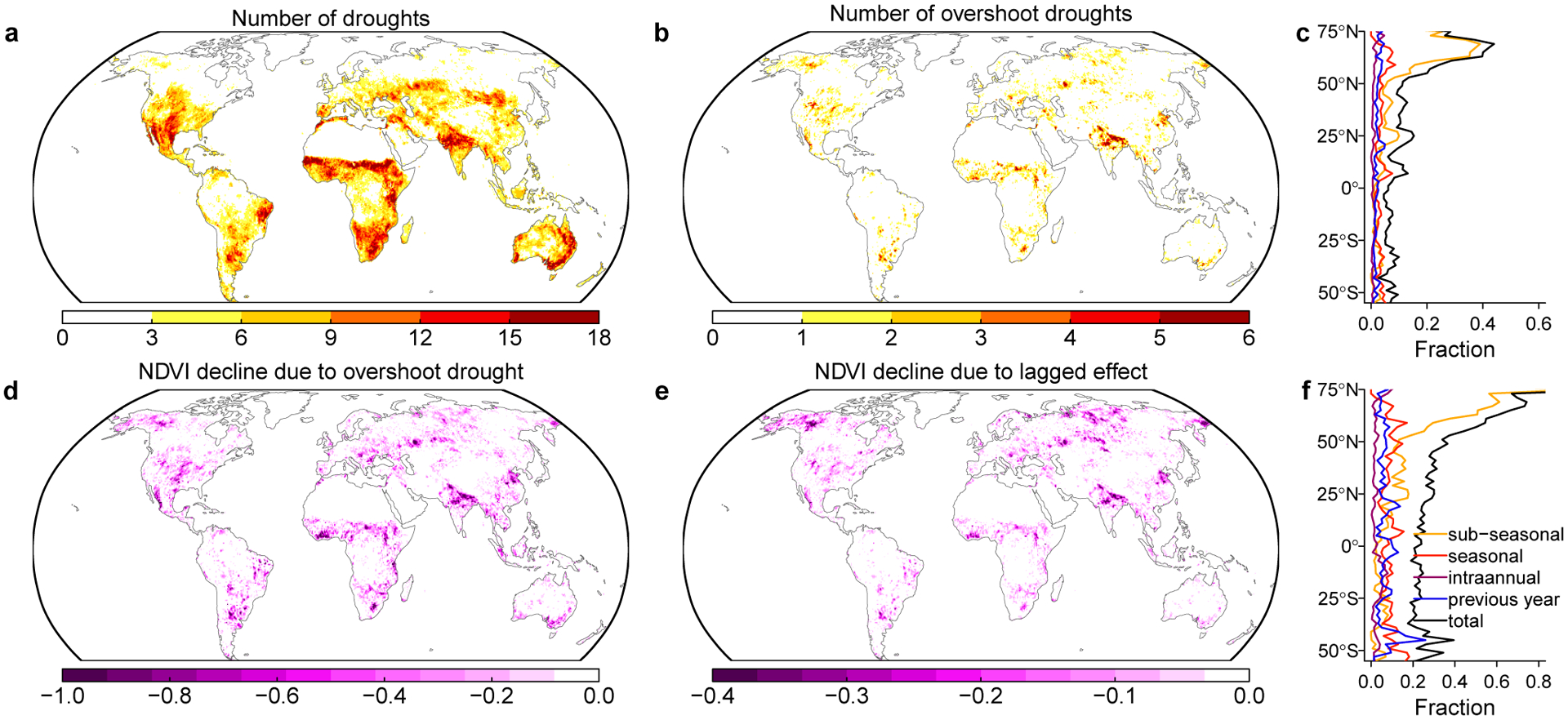
a,b number of droughts and number of overshoot droughts during 1981 to 2015. c latitudinal distribution of the fraction of drought related to overshoot. The black line indicates the total overshoot fraction, colored lines indicate the fraction of overshoot happening at sub-seasonal to interannual scales (see Methods). d summation of NDVI declines for the overshoot drought events. e NDVI declines caused by the lagged adverse effect (direct overshoot impact). f fraction of total overshoot contribution to the NDVI decline (black) and fraction for each overshoot component (colored lines). The drought events are identified by a combination of climatological drought severity and their impact on vegetation (see Methods).
Controlling factors and underlying mechanisms
To understand which factors contribute to the number and impact of overshoot droughts, we built random forest models using various climate variables and ecosystem characteristics to predict the spatial pattern of the fraction of drought related to overshoot and the fraction of lagged adverse effects to total drought impact (see Methods). The resulting models can explain 63.9% and 50.5% of the spatial out-of-bag variance for the fraction of overshoot number and impact, respectively. Based on these models, we obtain the rank importance of variables that drive these spatial patterns, and the partial dependence of the fraction of overshoot number and impact along each variable (Fig. 2).
Fig. 2 |. Response functions for the fraction of drought events related to overshoot and fraction of drought impact attributed to overshoot.
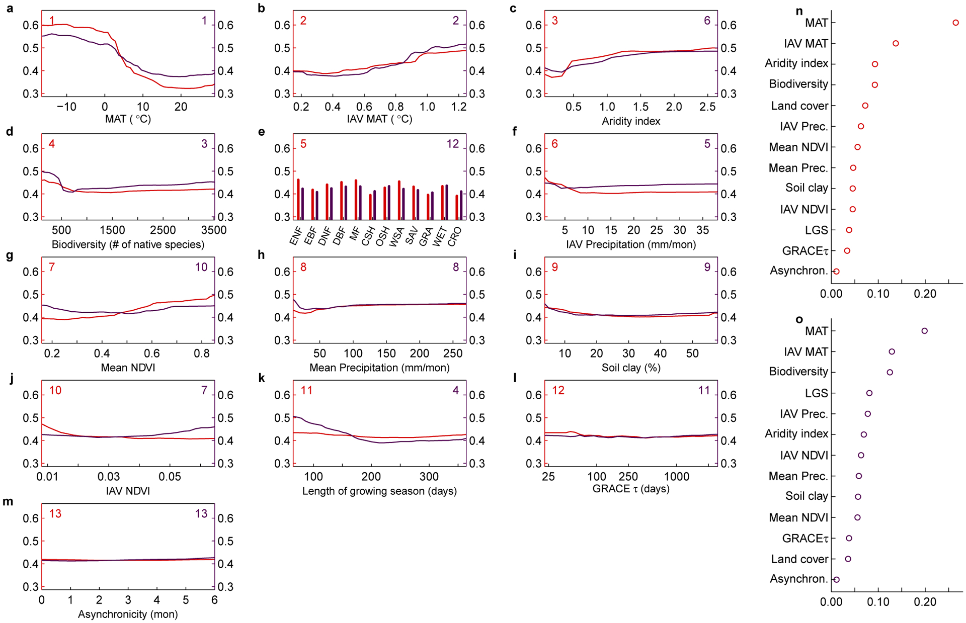
a-m, Response functions obtained from the random forest models. The left axis shows the fraction of drought events related to overshoot and the right axis shows the fraction of lagged adverse impact to total NDVI decline for overshoot droughts (see Methods). The numbers in the top-left and top-right corners indicate the order of importance for predicting the fraction of occurrence and lagged impacts of overshoot drought, respectively. n-o normalized variable importance for predicting occurrence fraction (n) and impact fraction (o). MAT: mean annual temperature; IAV: inter-annual variability; LGS: length of growing season; GRACEτ: terrestrial water decay time from GRACE. Biodiversity is assessed by the number of native species within each grid cell (see Methods). Types of major land cover types in e are evergreen needleleaf forest (ENF), evergreen broadleaf forest (EBF), deciduous needleleaf forest (DNF), deciduous broadleaf forest (DBF), mixed forest (MF), closed shrubland (CSH), open shrubland (OSH), woody savannas (WSA), savannas (SAV), grassland (GRA), wetland (WET) and cropland (CRO).
Overshoot droughts are more prevalent in stressed or seasonally stressed environments, usually with a shorter growing season (Fig. 2k). Positive climate anomalies in stressed environments can act as a stimulus for vegetation growth, allowing temporary exceedance of climatologically-defined ecosystem carrying capacity. Temperature stress, in comparison to water stress, can lead to more frequent and greater impacts of overshoot drought events (Fig. 2a,h). In cold regions (mean annual temperature less than 0°C), temperature is the primary limiting factor for both vegetation phenology and productivity during the entire growing seasons14,15. A positive temperature anomaly in the early growing season exponentially increases water consumption16, potentially leading to higher drought risk and stronger lagged effect. In comparison, mean annual precipitation plays a less important role. This is likely due to the fact that soil water is mostly low and has limited buffering capacity in dry regions, ecosystems are therefore more responsive to concurrent precipitation anomalies and relatively less dependent on the lagged effect17. As expected, the number and impact of overshoot drought events also increases with larger interannual variations of mean annual temperature (MAT) but much less with precipitation (Fig. 2b,f). Increases in climate variability not only increase the chances of a more favorable environment for plant growth in earlier periods, but also induce more frequent extreme heat and dry anomalies, leading to water deficit and potential drought.
Ecosystem biodiversity also plays a critical role in regulating overshoot drought occurrence. The number and impact of overshoot droughts decrease when the number of native species is greater than 500 (Fig. 2d). Low biodiversity is associated with synchronous plant behavior (e.g., expansive growth when the environment is favorable, and soil water depletion at similar rooting depths18). In addition, ecosystems with low biodiversity are expected to have weaker drought resistance, and thus lagged adverse effects tend to have a greater proportional impact19. Vegetation coverage, represented by mean annual NDVI, also positively affects the number of overshoot drought events (Fig. 2g). Higher vegetation coverage increases the plants’ role in linking the energy and water fluxes between soils and the atmosphere20. Anomalies in high vegetation coverage ecosystems would therefore have a greater impact on soil water and are more likely to induce a lagged adverse effect. Land cover type also plays an important role, with a higher number and impact of overshoot drought events for boreal forest and woody savannas (Fig. 2e).
In contrast, soil characteristics (clay fraction), terrestrial water decay time estimated from Gravity Recovery and Climate Experiment satellites (GRACEτ, Methods), and asynchronicity between peak temperature and precipitation show little role in determining the number and impact of overshoot drought events. We also test the robustness of these results by predicting the absolute overshoot drought number and lagged effect instead of their fractions with two other random forest models, and find similar environmental dependences (see Methods, Supplementary Fig. 4).
Overshoot and compound drought and heat
We further analyze the temporal occurrence of overshoot droughts. In the northern mid- to high-latitudes (>30°N), 51.2% overshoot drought events happen in July and August (Fig. 3a). For the Southern Hemisphere, two peaks can be observed in March and September, which is likely due to the double growing season experienced in many water-limited regions. Similar patterns can also be observed in parts of dry Mediterranean climate regions in the Northern Hemisphere, where overshoot drought may happen in either peak growing season. We also compare the start date for overshoot drought and non-overshoot droughts. To make these dates comparable across space, they are normalized by the peak growing season, and the results are summarized in four aridity regions (Fig. 3b–e). For dryland regions, non-overshoot droughts are more likely to happen before the peak growing season, while overshoot droughts are more likely to happen in the mid- to late growing season (Fig. 3b–c). These significant differences in drought timing (P<0.0001, paired two-sided t-test) also suggests that overshoot droughts are more likely to happen in warmer months, especially for semi-arid and dry sub-humid regions (Fig. 3f–i, Extended Data Fig. 5a). Considering the positive temperature anomalies during the drought period, overshoot droughts tend to have higher risk of extreme temperature. This compound drought and heat can be detrimental to ecosystem functioning and related ecosystem services, particularly for the mid-latitude semi-arid to dry sub-humid regions21–23, which are also major crop production areas and densely populated.
Fig. 3 |. Temporal distribution and temperature differences for overshoot droughts.
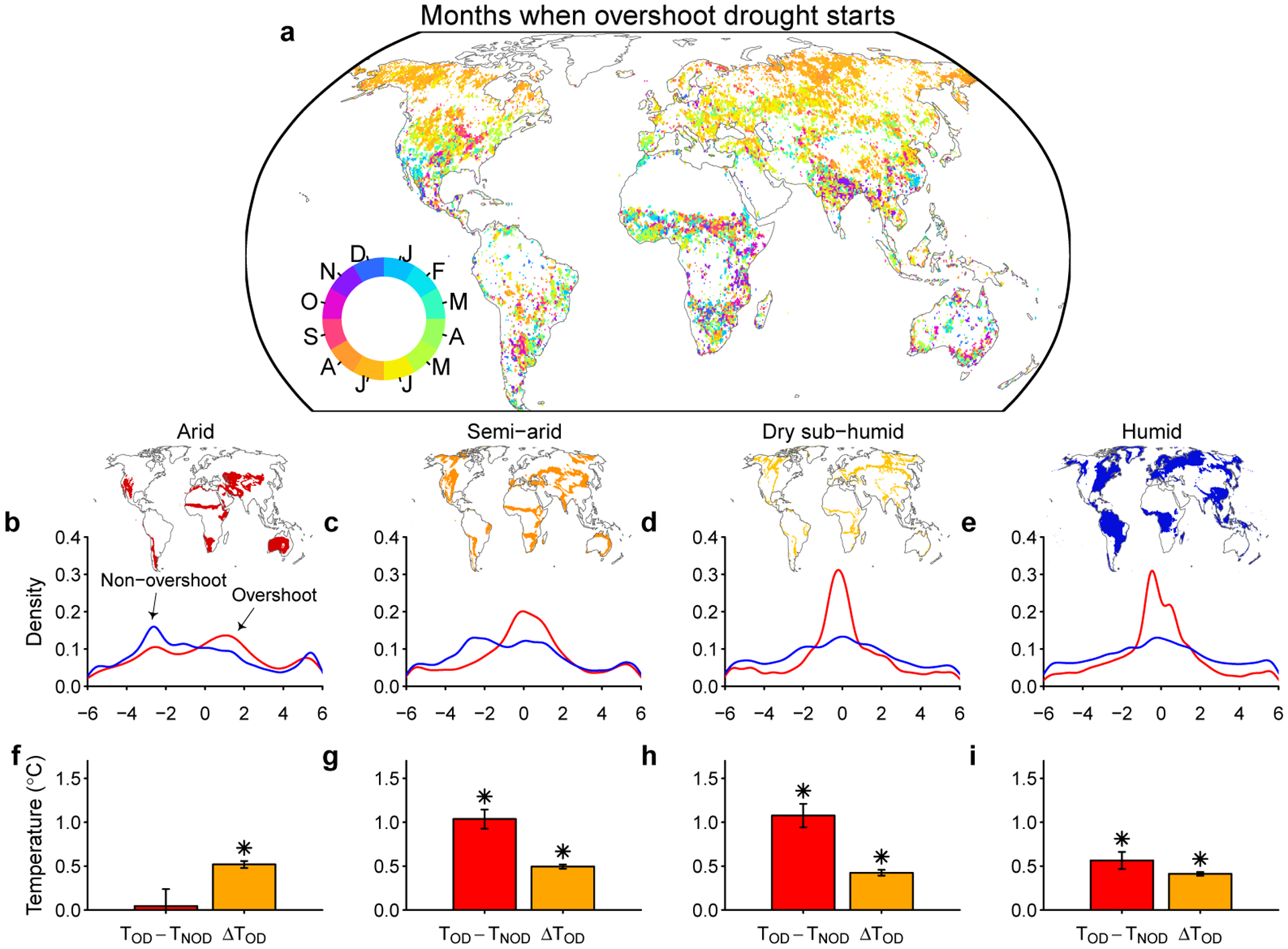
a Months when overshoot droughts are most likely to start. b-e temporal distribution of overshoot (red) and non-overshoot (blue) droughts for four aridity regions using peak growing season as a reference (b arid, c semi-arid, d dry sub-humid, e humid). Negative values indicate the droughts happen before the growing season peaks (in months). f-i temperature differences for overshoot droughts for four aridity regions. Red bars indicate the mean climatological temperature difference for overshoot (TOD) and non-overshoot (TNOD) drought events. Climatological temperature for each month is calculated during 1981–2015 for each pixel. Orange bars indicate the mean temperature anomaly for overshoot droughts after removing the climatological mean (ΔTOD). Error bars indicate the 95% confidence interval from bootstrap analysis (n=2000). An asterisk above the bar indicates the temperature difference is significantly different from zero (P<0.0001, paired two-sided t-test).
Overshoot and the development speed of drought impacts
Globally, overshoot droughts are associated with a faster NDVI decline than non-overshoot droughts (P<0.0001, paired two-sided t-test) (Fig. 4). Similar patterns can also be found if comparing the maximum NDVI decrease speed or the NDVI changes at the zero-crossing month (Extended Data Fig. 6). This faster decrease in NDVI is often accompanied with larger differences in NDVI anomalies between the start and end of the drought development period (Fig. 4b–g). Using soil moisture data from ERA5 reanalysis24 and a machine learning approach25, we also find faster soil moisture decline for overshoot droughts than non-overshoot droughts (P<0.0001, paired two-sided t-test) (Extended Data Fig. 7). However, the differences in soil moisture changes are much smaller than the differences in vegetation declines (P<0.0001, unpaired two-sided t-test), potentially because the interannual variations of vegetation is not used as a forcing in these datasets, and their effects on soil moisture may thus be underestimated.
Fig. 4 |. A comparison of the development speed of drought impacts on vegetation between overshoot and non-overshoot drought events.
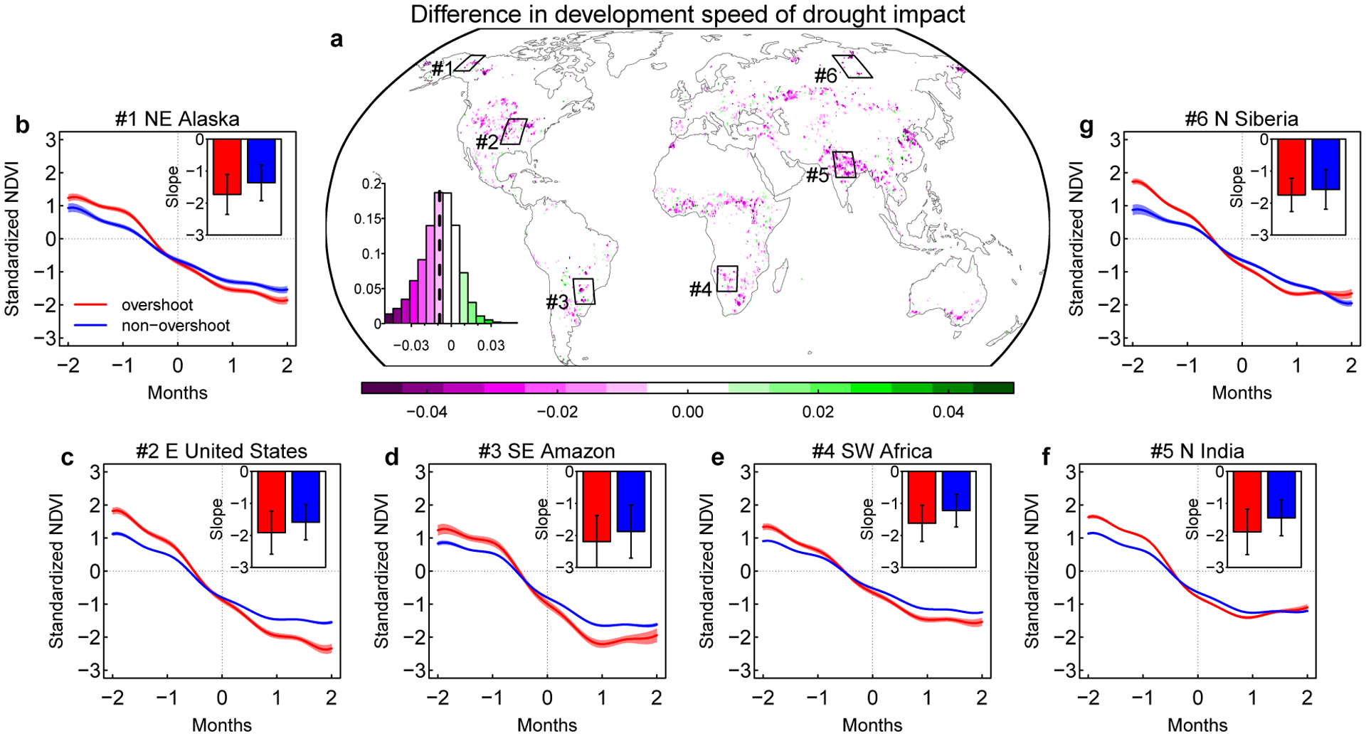
a Differences between mean development speed of drought impacts for all overshoot and non-overshoot drought events. The inset in a shows the histogram of these differences, with the dashed vertical line showing the mean value. The development speed for each drought event is calculated as the median value of the NDVI change rate during the drought development period. b-g changes in standardized NDVI anomalies during drought development periods for six regions across the globe. The de-seasonalized detrended NDVI anomalies are standardized using their standard deviations so that changes can be compared across pixels in each region. Month 0 corresponds to the start of the drought event (first negative NDVI anomaly). Subsets in each region show the comparison between NDVI decline speed during the drought development stage for overshoot (red) and non-overshoot (blue) drought events (see Methods). The mean and s.d. are calculated from all drought events within the region.
Due to the rapid onset and intensification of vegetation deterioration, the majority of overshoot droughts we identify can also be classified as flash droughts26,27. Flash droughts occur most frequently in mid latitude semi-arid or dry sub-humid regions where overshoot impacts are dominated by the sub-seasonal and seasonal lagged effects (Extended Data Fig. 3). Most overshoot droughts develop very quickly (mostly 2–3 months), and are on average 1–2 months shorter than non-overshoot droughts in these semi-arid regions (Extended Data Fig. 8).
In addition, overshoot droughts usually lead to stronger drought impacts for dry sub-humid and humid regions, as shown by a more negative NDVI anomaly compared to the standardized precipitation evapotranspiration index (SPEI) anomaly (Extended Data Fig. 9). SPEI is a widely used drought severity indicator which calculates the standardized surface water balance anomaly from meteorological variables. To understand how overshoot modulates the drought severity (assessed by minimum SPEI) and impact (assessed by minimum of standardized NDVI, NDVIz) relationship, we build three nested linear models to predict NDVIz anomalies from SPEI values during droughts. The first model does not consider overshoot effect. The second considers the effect on intercepts only, and the third considers the effect on both the regression slopes and intercepts (Methods, Extended Data Fig. 10). The results from this model comparison can be summarized into five types of severity-impact responses (see Methods, Fig. 5b). For about a quarter of the area where the three models are evaluated, overshoot exacerbates drought impact to the same degree across different drought severities (Type 1 in Fig. 5). The nested models predict an additional NDVIz decline of −0.58±0.30. In another quarter of area, overshoot leads to stronger impact when drought severity is low, causing a decrease of NDVIz by −0.07±0.28 (Type 2 in Fig. 5). By contrast, only 3% of area indicates overshoot has stronger impact when drought severity is high, with an additional NDVIz decline by −0.27±0.24 (Type 3 in Fig. 5). Overshoot alleviates the drought impact for only 4% of the area (Type 4 in Fig. 5). This may be due to a mismatch in timing when drought or overshoot impact reach their maximum.
Fig. 5. NDVI changes due to overshoot.
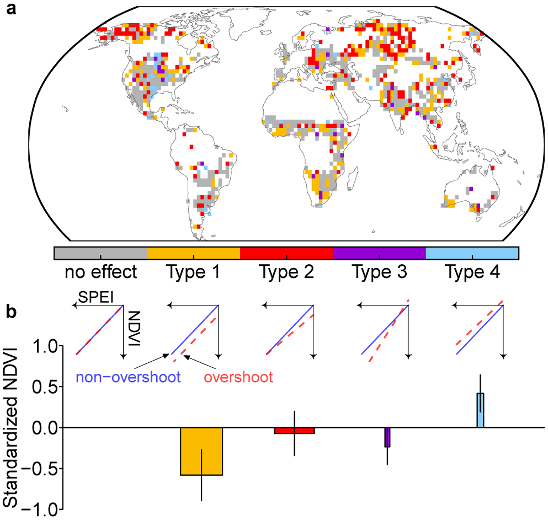
a The spatial pattern of different types of overshoot effects on modulating drought impact based on results from three nested models. White area indicates insufficient samples for model fitting (see Methods). b Average NDVI changes due to overshoot. These changes are predicted by the nested models together with the mean SPEI values for all overshoot droughts. The widths of the bars indicate the areal fractions for each type. Error bars indicate the s.d. of spatial variations. The subplots in b show five types of responses of how overshoot modifies the NDVI and SPEI relationship. These five types of responses differ in their regression intercepts and slopes for overshoot and non-overshoot droughts. The x-axis indicates the drought severity (minimum SPEI values during drought) and the y-axis indicates the drought impact (minimum standardized NDVI). The direction of arrows indicates a decrease for both (stronger drought severity and impact).
Our analysis, based on a dynamic statistical learning approach applied to long-term satellite vegetation records, provides a global understanding of the role of vegetation structural overshoot in the timing, speed and impact of drought events. Overshoot droughts are found to develop faster and be more likely to compound with extreme heat than non-overshoot droughts, exacerbating the drought impact on ecosystem function and the associated societal services. Overshoot droughts are also expected to be associated with increased competition, changes in species composition and functional groups. It is not possible however to analyze these ecological processes at global scales in our study and they therefore warrant further analysis. Soil water balance may be the key to link the lagged adverse effects, but land-atmosphere feedbacks28,29 and other processes such as plant phenology30,31, and fire disturbance play potentially important roles. Current drought indices, including those relying on potential evapotranspiration, do not consider vegetation status in calculating the water balance, may therefore underestimate drought severity when structural overshoot happens. Global climate change can promote faster vegetation growth32 and soil water depletion33, together with more frequent and severe climate extremes, potentially increasing the overshoot drought occurrence and impact. Continuous satellite monitoring and improved model simulation are needed to help better understand the changes of overshoot and improve the prediction of future drought impacts.
Methods
GIMMS NDVI and Climate datasets
We use the normalized difference vegetation index (NDVI) from Global Inventory Monitoring and Modeling System (GIMMS) 3gv1 (1981–2015, ref13) which provides long-term records for vegetation activity. NDVI is a remotely sensed indicator based on the unique spectral characteristics of vegetation and has been demonstrated to be strongly related to ecosystem leaf area index and photosynthetic capacity34–36. It can therefore represent the aggregated ecosystem response to climatic anomalies and drought stress. This dataset is first quality checked and aggregated to monthly 0.5° × 0.5° resolution to match the resolution of other datasets and to reduce the uncertainty. In many northern regions, the quality flags are not always effective, especially when mixed snow pixels exist. Since the DLM is sensitive to these de-seasonalized anomalies, and drought and water limitations are not likely to happen during these cold and snow-covered periods, we therefore use an additional temperature threshold to filter out these potential contaminated pixels: if the mean air temperature for a specific month is below 0 °C, the land surface may be covered by snow and the corresponding NDVI is set to NA.
We use both precipitation and temperature as environmental variables in the DLM. The precipitation dataset is from the Global Precipitation Climatology Centre (GPCC)37. This dataset provides monthly precipitation at a 0.5° × 0.5° spatial resolution. The dataset is generated using a spatial statistical method based on observations from global gauge network which extends beyond Global Historical Climatology Network (GHCN). Compared to other precipitation datasets (for example, the Climatic Research Unit gridded Time Series (CRU TS4.04)), this dataset uses more stations and is often considered to be a more reliable estimate of precipitation at the global scale39. We use the monthly air temperature dataset from CRU TS 4.04 (ref38). CRU generates gridded climate dataset from weather station data and a spatial statistical method. We also use a standardized precipitation evapotranspiration index (SPEI40) dataset for drought identification and drought severity assessment. SPEI is a widely used climatological drought index that calculates the standardized water balance anomalies (precipitation minus potential evapotranspiration) at different time scales. It is therefore an optimal index to evaluate the drought severity-impact relationship and the role overshoot plays in this process. We use a 3-month SPEI dataset based on the CRU dataset so that it can capture the short-term water deficit.
Bayesian multivariate dynamic linear model (DLM)
The multivariate dynamic linear model is a type of linear model for time series analysis12. Compared to a multivariate regression model, it allows the regression coefficients to change over time, which can better capture the time-varying relationship between vegetation status in the past and at present. This method was introduced by Harrison and Stevens41 and well documented by West and Harrison12. In this study, we modify the model structure used by Liu et al. (ref42), by further considering the lagged effect of vegetation anomalies from previous months along with concurrent climate anomalies. For each pixel, the DLM predicts the time series of the target variable (yt, satellite retrieved NDVI) using an observation equation (Eq. 1) and a state evolution equation (Eq. 2):
| (1) |
| (2) |
where yt is the observed NDVI at each month t after removing the mean. Ft is a vector consisting of three components, a constant for local mean and trend (Ftrend = [1,0]), a constant for three seasonal components (Fseas = [1,0,1,0,1,0]), and a regression component including the temperature, precipitation and NDVI anomalies (δ) from previous months which change with time t (Freg,t = [δTempt, δPrect−1,t−3, δNDVIt−1, δNDVIt−2,t−3, δNDVIt−4,t−6, δNDVIt−7,t−12, δNDVIt−13,t−24]).
The subscript of each variable indicates the starting and ending months used to calculate the mean value, using the de-seasonalized and detrended temperature, precipitation and NDVI. We do not consider radiation in this default model setup because the interannual variations of radiation is small and can have strong correlation with temperature or precipitation at monthly scale. θt is the state vector at time t, which also consists of three components: coefficients representing local mean and trend, coefficients representing seasonal dynamic and regression coefficients for the previous months’ NDVI, as well as environmental factors (previous months precipitation, current month temperature). υt is the state evolution noise at time t assuming it has a zero mean with a Gaussian distribution. G is a known state evolution matrix that is block diagonally connected with three small matrices, corresponding to the local mean and trend component, the seasonal component, and the regression component. wt is the state evolution noise at time t, following a zero mean multivariate Gaussian distribution. Starting with non-informative priors of θ0 and noises of υt and wt, we estimate the posterior distribution of θt using the forward filtering method. This method uses Kalman Filtering to get the posterior of yt, and takes a step further to back propagate the difference between prior and posterior estimates of yt to get the posterior estimates of θt. In this study, we focus on the posterior estimates of the regression coefficients for the previous months’ NDVI, named DLM sensitivities. These sensitivities, together with their corresponding NDVI anomalies (contributions to the predicted current month NDVI from each of the previous months’ NDVI, e.g., δNDVIt−2,t−3 × θt) were used to identify overshoot droughts. Since the DLM uses a Kalman Filter at each time step, in order to get a reliable prediction of the coefficient, especially in the early study period, we use a “spin-up” period by recycling the first five years (1981–1986) of satellite NDVI and climate observations two times prior to the start of the dataset. It should be noted that although the model is a class of “linear models”, its sensitivities change through time, and thus can capture temporal non-linearity. A detailed description of this method can be found in the Supplementary Text 1. In addition to this “default model” setup which considers both temperature and precipitation in the regression component, we also test a “reduced model” which does not consider temperature, and an “extended model” that considers precipitation, temperature, and radiation. A detailed description on these experimental setups together with other sensitivity analysis can be found in Supplementary Text 2.
Drought and overshoot identification
We use a combination of SPEI and NDVI together with outputs from the DLM to identify drought events. Both indices are directly calculated from observations and represent the climatological drought severity and the drought impact on vegetation, respectively. After the NDVI time series for each pixel is decomposed by the DLM, we identify all negative anomalies from the de-seasonalized and detrended NDVI (original NDVI time series minus trend and seasonal components obtained from DLM decomposition). For each consecutive negative NDVI anomaly time window, a minimum value is first retrieved. A drought starts when the NDVI anomaly turns negative and ends when the NDVI anomaly recovers above 70% of the minimum value. Three criteria need to be met in order to be considered as a drought event: (1) drought should be at least two months long and the minimum NDVI anomaly should be smaller (more negative) than 10% of the mean NDVI in order to exclude events due to random noise in NDVI; (2) the average SPEI during the corresponding period is below −0.5. It should be noted that we used a relaxed threshold for SPEI (“−0.5” compared to commonly used “−1”), since overshoot droughts may happen with only moderate precipitation decline; (3) the temperature component during the drought period should be greater than the precipitation component (less negative) or the temperature sensitivity (coefficient for δTempt) should be negative. This is to exclude the NDVI decline due to low temperature rather than low soil water.
Overshoot in this study is defined as vegetation’s temporary exceedance of the ecosystem carrying capacity, which leads to increased soil water consumption and causes a lagged adverse effect on latter vegetation activity due to water stress. It should be noted that because of the seasonal dynamics of vegetation and climatic factors, the carrying capacity, i.e., the maximum plant canopy that can be supported, is also time-varying. Soil water dynamics contain the overshoot information but cannot be directly observed, so the approach we use to identify structural overshoot is to examine the lagged adverse linkage between de-seasonalized anomalies of NDVI.
In practice, after drought events are identified for each pixel, we calculate the average NDVI anomaly and DLM sensitivity during each drought period for each of the four previous-month NDVI components, i.e., previous 2–3 months, previous 4–6 months, previous 7–12 months, and previous 13–24 months (Extended Data Fig. 1). For each drought event, if any of the four previous-month NDVI components have a positive anomaly associated with a significantly negative (CI=0.9) sensitivity coefficient, that is, the total contribution (the product of NDVI anomaly and sensitivity) to the prediction of current NDVI is negative, this NDVI component is regarded as an overshoot component. For a drought event, if the summation of all overshoot component contributions is greater than the non-overshoot contributions by absolute value, and the minimum of the overshoot component is less than −0.01, this drought event is considered as an overshoot drought event. Since we use several arbitrary thresholds in the drought and overshoot drought identification, we also test the uncertainties caused by the model structure and thresholds chosen. The results show that different models and thresholds can affect the absolute number of droughts and overshoot droughts, however, the spatial patterns are quite similar and the fraction of overshoot drought numbers to total drought numbers is conservative, ranging from 9.93% to 18.49%, with a median value of 11.22%. Detailed information is provided in Supplementary Text 2, Supplementary Table 1 and Supplementary Fig. 5–11. In addition to GIMMS NDVI, we also use NDVI from the Moderate Resolution Image Spectrometer (MODIS) MOD13C2 and identify overshoot during 2000–2018. The resulting spatial patterns are similar with those obtained using GIMMS NDVI (Supplementary Fig. 12).
To understand the differences in development speed of drought impact between overshoot and non-overshoot drought, we first define a drought development period which begins with the monotonical decrease of the de-seasonalized detrended NDVI anomalies and ends when it reaches its minimum within a drought event. Within each drought development period, we first calculate the speed of changes as the differences in de-seasonalized detrended NDVI anomalies between months. We compare three metrics to characterize the development speed of drought impact: the speed of changes at its maximum (75 percentile), median (50 percentile) and at the zero-crossing month (i.e., when the NDVI anomalies shift from positive to negative).
Timing of overshoot
We identify the starting month for each drought event to examine drought timing. For each pixel, the average starting months for overshoot and non-overshoot drought events are calculated separately. We fit a probability density function (PDF) of the overshoot drought starting date for each pixel and determined the months when the probability reaches its maximum. Since December and January are also nearby months but the PDF cannot be correctly fitted under this condition, we shift the starting date by 3- 6- 9- months and fitted three other PDFs. The final starting date is determined by the month that corresponds to the maximum probability across all four PDFs. If the maximum probabilities for the four PDFs are the same, it indicates that the starting dates of overshoot drought do not have any tendency and this pixel is not used. This only happens for a very small proportion of the total area (~0.55%). To make these timings comparable across space, we normalize the starting months of each drought event by the peak growing season. These differences are then rescaled to −6 to +6 months.
Drought impact assessment
Drought impact on vegetation is often related to meteorological water deficit, however, this relationship may be altered when overshoot happens. We use three nested models to assess the overshoot impact on this relationship:
| (3) |
| (4) |
| (5) |
The first model (null model) only considers water deficit as indicated by 3-month SPEI. The second model assumes that when overshoot happens, it will change the intercept of the regression. The third model assumes that when overshoot happens, both the intercept and the sensitivity of SPEI will change. Since there is a limited number of overshoot drought events for each pixel, we evaluate these three models on 2.5° × 2.5° windows, so that each window has at least 10 overshoot droughts and 10 non-overshoot droughts during the study period. To make NDVI declines comparable within each window, the NDVI declines are standardized by the standard deviation of de-seasonalized detrended anomalies (NDVIz, z-score). The best model is selected based on an ANOVA comparison, second and third models are only selected when they are significantly better than the first model (p<0.1).
Based on the comparison of these three models, we categorize overshoot impact into five groups (Fig. 5). (1) overshoot has no effect on the NDVI-SPEI relationship. This is considered when the first model is chosen; (2) overshoot decreases the intercept of the NDVI response to SPEI, but the NDVI response to SPEI remain the same. This is considered when the second model is chosen and coefficient b is negative; (3) overshoot decreases the intercept of the NDVI response to SPEI, but the sensitivity of NDVI to SPEI is reduced. This is considered when the third model is chosen and both coefficient b and c are negative. (4) overshoot increases the intercept of the NDVI response to SPEI, and the sensitivity of NDVI to SPEI is increased. This is considered when the third model is chosen and both coefficient b and c are positive. (5) overshoot alleviates the drought impact. This is considered when all other cases happen. To assess the overshoot impact on drought, we predict the effect related to overshoot based on the best model selected and average SPEI values for all overshoot drought events within this 2.5° ×2.5° window.
Randomized experiment
We set up a randomized experiment to test if the DLM can effectively capture the linkages between the previous positive NDVI anomalies and current NDVI decline, that is, the overshoot. It has the following four steps:
Twelve months are grouped into 6 groups, with each group have two consecutive months (e.g., January and February, March and April).
NDVI, temperature, and 3-month precipitation and SPEI for each group are shuffled together across years, so that the NDVI for each month still corresponds to the temperature and precipitation for that month, and their relative positions within a year remain unchanged, e.g., July and August from 2012 may be swapped to July and August, 1998, following May and June from 2007.
Using this randomized dataset, we again run the DLM model and identified the drought and overshoot drought events for 1981–2015.
This process is repeated 5 times with different random seed for the step (2). After the drought and overshoot drought events are identified, we swap them back to their original position so that they are comparable between randomized experiments. If three out of five experiments identify any two months as a drought event, this event is considered as a valid drought event. If three out of five experiments identify a drought event as an overshoot drought event, this event is considered as a valid overshoot drought event.
We swap the months by 2-month group sizes because during the drought identification step, a negative anomaly should be at least two-month long so that it can be considered as a potential drought event. This step should have limited effect on drought identification since droughts are identified based on NDVI with concurrent climate anomalies which are swapped together. In the randomized experiment, however, this random swap is likely to break up most of the lagged effects.
We also test if the lagged effect can be partially retained if we choose larger group sizes. To do so, instead of swapping the NDVI by two-month groups in step (1), we use larger group sizes of 6-month, and 24-month during the swap. For example, March to August in 2012 will be moved together to March to August in 1999 (6-month group) or September 2010 to August 2012 will be moved together to September 1982 to August 1984 (24-month group). By using larger groups, partial lagged effects may be retained, for example, the lagged effects at sub-seasonal scale may be kept using the 6-month group size, and the effect at intra-annual scale may be kept if we use 24-month group size.
We find that when using a group size of two months, the spatial pattern of drought numbers does not change much, while most of the overshoot droughts are no longer identified. With the increase of the group sizes, more overshoot drought events are identified, and the spatial patterns become similar to the one we obtained without randomization. This suggests the DLM can effectively capture the lagged effect and help identify overshoot drought events. More detailed information is provided in Supplementary Text 3 and Supplementary Fig. 14–16.
Synthetic data experiment
We also generate a synthetic dataset to test if overshoot drought events can be effectively identified using our methodology. To do this, we first build a simple vegetation model that considers both the direct effect of environment and the lagged effect of previous months NDVI through soil water dynamics (Supplementary Text 4). We focus on the 2012 overshoot drought in central US8. Using this simple model, we set up four different scenarios to simulate vegetation dynamics, and applied the overshoot identification algorithm used in this study:
Control run, spring warming and low summer precipitation
No spring warming, low summer precipitation
Spring warming, normal summer precipitation
Spring warming, abundant summer precipitation but with other disturbances
These four scenarios differ in their environmental drivers and, consequently, NDVI anomalies simulated by the simple model. Based on the synthetic data, only Scenario 1 is considered as an overshoot drought event, while for the other three, they either do not exhibit a lagged adverse effect or the NDVI decline is not caused by drought. It should be noted that in the real world, Scenario 3 may develop into overshoot drought for certain ecosystems. Our objective here is not to verify the performance of the simple model, but to test the effectiveness of the overshoot identification algorithm based on these synthetic data. Our overshoot identification algorithm correctly identifies the overshoot drought in Scenario 1, and correctly identifies the other scenarios as non-overshoot droughts (Supplementary Fig. 17–19). This experiment demonstrates the effectiveness of our algorithm in identifying the overshoot drought. More detailed information is provided in Supplementary Text 4 and Supplementary Fig. 17–19.
Machine learning models to predict the numbers and impacts of overshoot drought events
We use two random forest algorithms with 13 independent variables each to predict the fraction of drought events related to overshoot and the fraction of lagged effect to the total impacts of overshoot droughts, respectively. The 13 shared variables include climate variables, e.g., mean annual temperature (MAT), interannual variation of MAT, mean precipitation, interannual variation of precipitation, asynchronicity between the months of maximum temperature and precipitation; ecosystem characteristics, including biodiversity, i.e., number of native species within a grid (Data available from http://ecotope.org/anthromes/biodiversity/plants/data/), mean NDVI, interannual variability of NDVI, length of the growing season (from MODIS derived phenology, data available from https://vip.arizona.edu/); hydroclimate indicators, e.g., aridity index (precipitation over potential evapotranspiration), terrestrial water decay time from GRACE (GRACE τ)43; and soil characteristic, e.g., the fraction of clay calculated as the average of clay fraction for the top layer and the lower layer (data from Regridded Harmonized World Soil Database v1.2, https://daac.ornl.gov/SOILS/guides/HWSD.html). The climate variables are all calculated using the CRU dataset during 1982–2015. As the contribution of one precipitation event to the total water storage decays exponentially over time, GRACEτ describes the time length (in days) when the contribution decreases to 1/e (≈ 37%) of its initial value. Drought recovery time44 and elevation are also tested in the model, but both showed very little contribution (<0.001) and are not used in the analysis. In addition to these two random forest models, we also build two other models which directly predict the overshoot numbers and lagged impacts, with the total drought number and total NDVI decline during overshoot droughts as additional independent variables, respectively.
The random forest is a machine learning algorithm consisting of multiple regression tress using bootstrapped samples. In this study, each random forest consists of 500 regression trees with a leaf node size no smaller than 5. A regression tree recursively splits samples into two categories (i.e., branches) using a binary rule at each step (for one independent variable), minimizing the variance within each branch. Based on the number of times each variable is used for the split, the variable importance metric can be calculated using the fitted random forest and the entire dataset. A larger number of splits indicates the variable is more important for the prediction of the response variable. The variable importance factors are normalized to unity (summation equals to one) for the two random forests.
The response function of fraction of overshoot drought numbers or impacts to each individual factor is shown as a partial dependent plot (PDP). The PDP calculates the predicted mean response of the target variable (e.g., number or impact of overshoot drought) to one independent variable (e.g., biodiversity), allowing other variables to change in their domain. In practice, it can be calculated as:
where is partial dependent function with respect to variable xs, xc are the other variables used in the random forest. The superscript “(i)” indicates one incident in the dataset.
Data Availability
The NDVI 3g v1 dataset is available at https://ecocast.arc.nasa.gov/data/pub/gimms/, the CRU climate dataset is available at https://crudata.uea.ac.uk/cru/data/hrg/, the GPCC precipitation data is available at https://www.dwd.de/EN/ourservices/gpcc/gpcc.html, phenology metrics derived from MODIS are available at https://vip.arizona.edu/viplab_data_explorer.php, the SPEI dataset is available at https://spei.csic.es/database.htmlt, the ERA5 soil moisture data is available at https://cds.climate.copernicus.eu/cdsapp#!/dataset/reanalysis-era5-land-monthly-means, the SoMo.ml soil moisture data is from https://www.bgc-jena.mpg.de/geodb/projects/Home.php. The source data for the figures are publicly available (https://doi.org/10.6084/m9.figshare.15086535)
Code Availability
The codes for the dynamic linear model and overshoot identification are available at https://github.com/zhangyaonju/Overshoot/.
Extended Data
Extended Data Fig. 1. Framework of DLM.
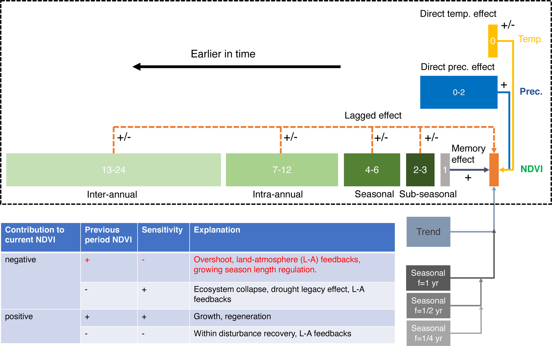
The DLM is composed of five terms, i.e., temperature component, precipitation component, direct and lagged vegetation components from previous months, trend component, and seasonal components. Numbers in the dashed box indicate the previous months used to calculate anomalies for NDVI, precipitation and temperature. The three seasonal components are harmonic functions with different frequencies.
Extended Data Fig. 2. An example of DLM decomposition of the NDVI time series, and the identification of an overshoot drought event.
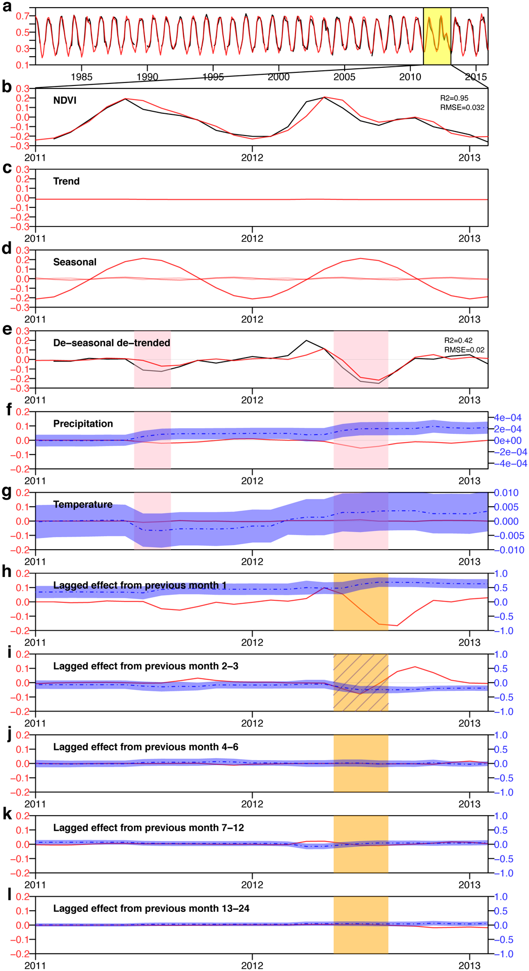
a Satellite retrieved time series of NDVI (black) and DLM predicted NDVI (red) in a grassland at Kansas, USA (latitude = 38.05°N, longitude = 96.44°W). b-k, Zoom-in comparison of DLM components during 2011–2012. b NDVI anomalies (NDVI minus long-term mean). c Trend component in DLM. d Three seasonal components. e de-seasonalized detrended NDVI observation (black, NDVI observation – trend and seasonal components) and predicted by the DLM (red, summation of precipitation, temperature components and previous month NDVI components). Pink shade indicates drought period. f Precipitation component (solid red line, left axis) and coefficient for precipitation (dashed blue line, right axis). g Temperature component (solid red line, left axis) and coefficient for temperature (dashed blue line, right axis). h-l Lagged effects (left-axis) and the corresponding coefficients (right-axis) from previous months (h), 2–3 months (sub-seasonal) (i), 4–6 months (seasonal) (j), 7–12 months (intra-annual) (k), 13–24 months (inter-annual) (l). Orange shades indicate the overshoot periods, with hatched ones indicate the overshoot components identified by our algorithm. Shaded areas around the blue dashed lines represent the 90% confidence interval. Take this 2012 summer drought event as an example, among the four lagged effects, previous month 2–3 shows a strong negative sensitivity and a negative contribution during the drought period, therefore it is considered as an overshoot component, its contribution also dominates all the lagged effects during the drought, this drought event is therefore considered as an overshoot drought event.
Extended Data Fig. 3. Contribution of each component to the overshoot number and impact.
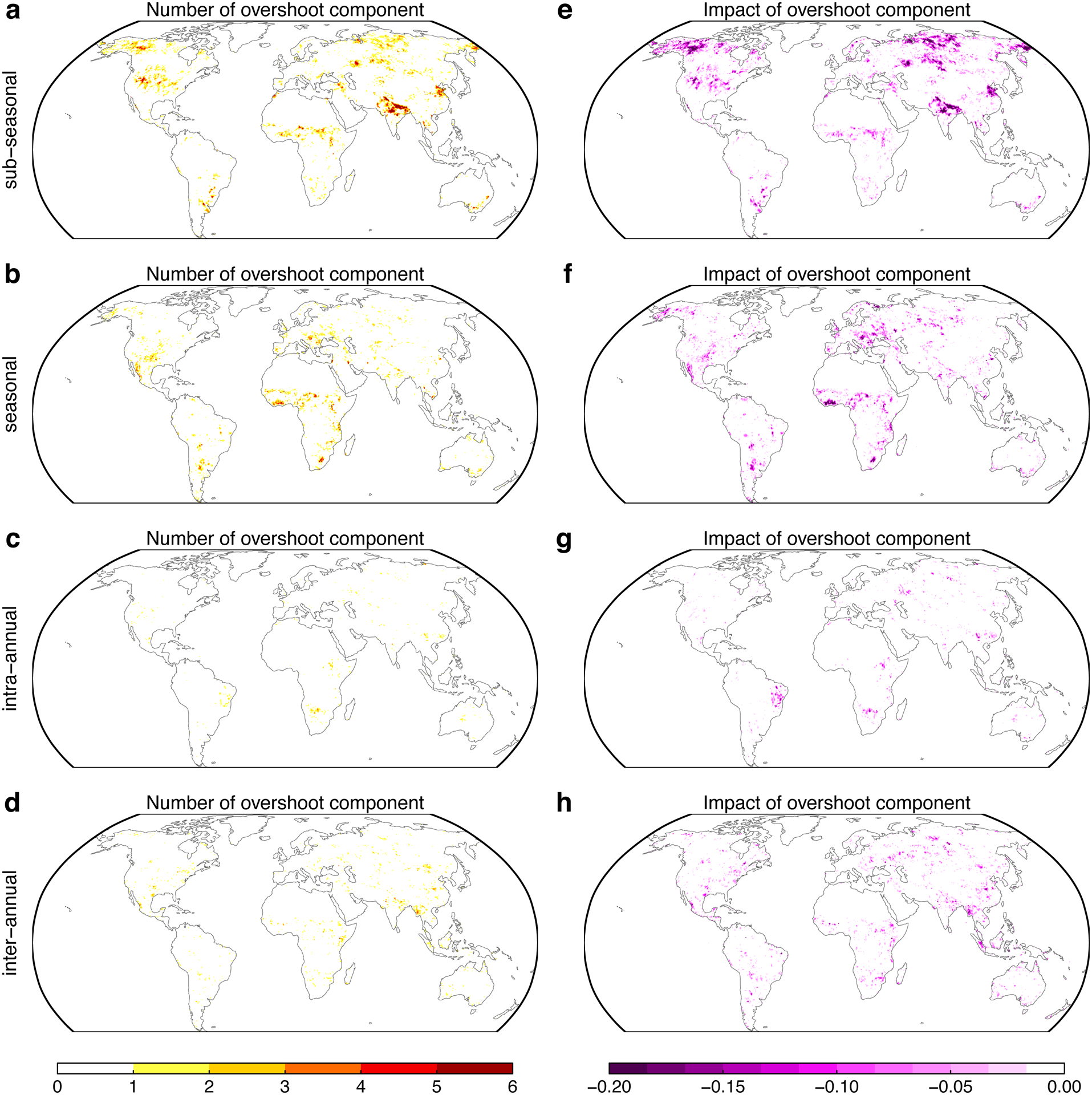
a-d Numbers of overshoot component at different time scales. e-h Impact of overshoot component at different time scales. Sub-seasonal indicates lagged effect from previous 2–3 months, seasonal indicates previous 4–6 months, intra-annual for previous 7–12 and inter-annual for previous 13–24 months.
Extended Data Fig. 4. The dominant overshoot component along the growing season length.
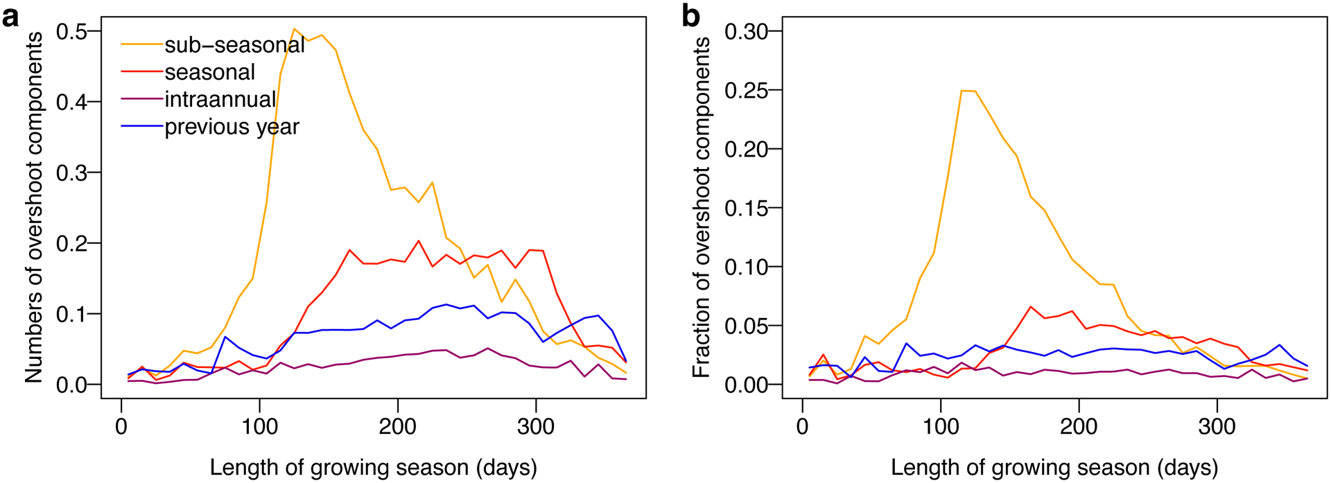
a Average number of overshoot component along the growing season length. b Average fraction of overshoot component numbers to drought numbers along the growing season length.
Extended Data Fig. 5. Differences in temperature for the overshoot droughts.
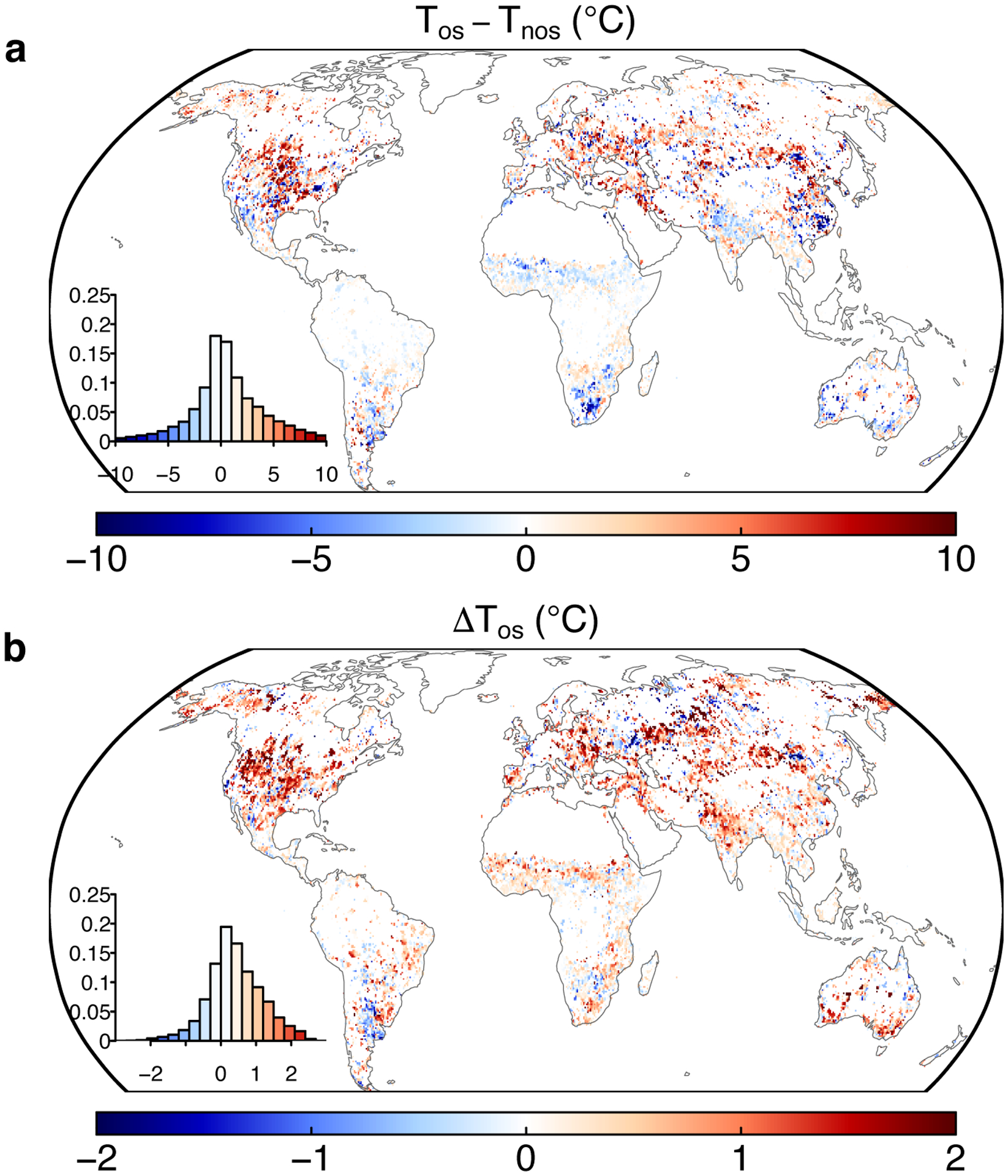
a Temperature differences between overshoot and non-overshoot droughts with the climatological means. b Average temperature anomalies relative to the climatological means for the overshoot droughts. Insets show the histograms of the anomalies.
Extended Data Fig. 6. Comparisons of the development speed of drought impact between overshoot and non-overshoot drought events.
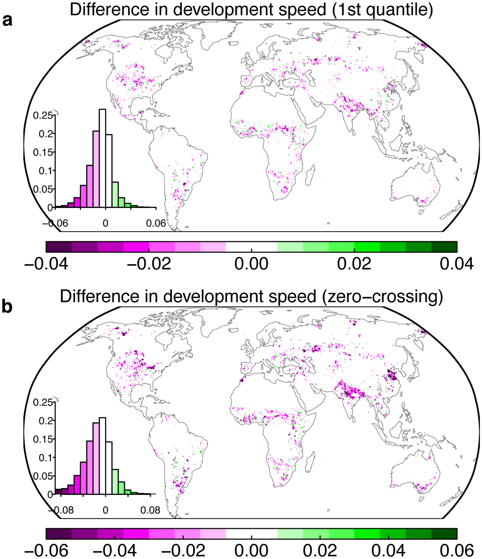
a The development speed is calculated as the 1st quantile value of the NDVI changes during the start of the decline to the minimum of the de-seasonalized detrended NDVI anomalies for each drought event. b Same as a, but using the change of NDVI at the zero-crossing date based on the de-seasonalized detrended NDVI anomalies. Insets show the histogram of the development speed.
Extended Data Fig. 7. Differences in the soil moisture declining speed between overshoot and non-overshoot drought events.
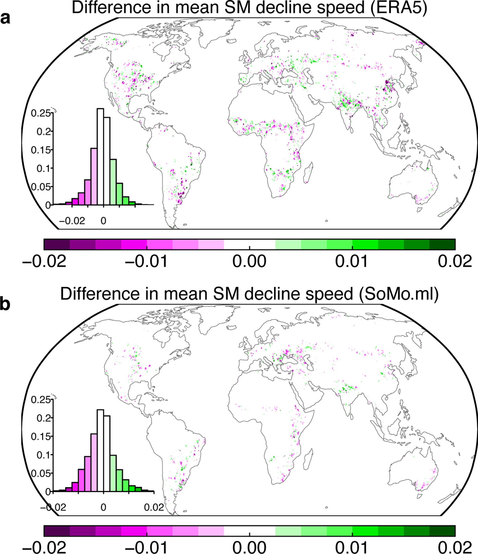
a Speed differences from ERA5 reanalysis soil moisture during 1981–2015. b Speed differences from a machine learning based soil moisture dataset (SoMo.ml) during 2000–2018. For ERA5, we used overshoot droughts derived from GIMMS NDVI (Fig. 1); for SoMo.ml, we used overshoot droughts derived from MODIS NDVI (Supplementary Fig. S12). Both soil moisture datasets were de-seasonalized and detrended first so that we only focus on the soil moisture anomalies. Soil moisture were integrated for top 1m for ERA5 and 0.5m for SoMo.ml. The pixel-level comparisons were only conducted when at least two overshoot and two non-overshoot drought events happened during the study period. The insets show the histogram of the differences, with negative values indicating average soil moisture declining speed is greater (more negative) for overshoot drought than non-overshoot drought. Units are in m3 m−3 mon−1.
Extended Data Fig. 8. Comparisons between the drought development time and drought lengths.
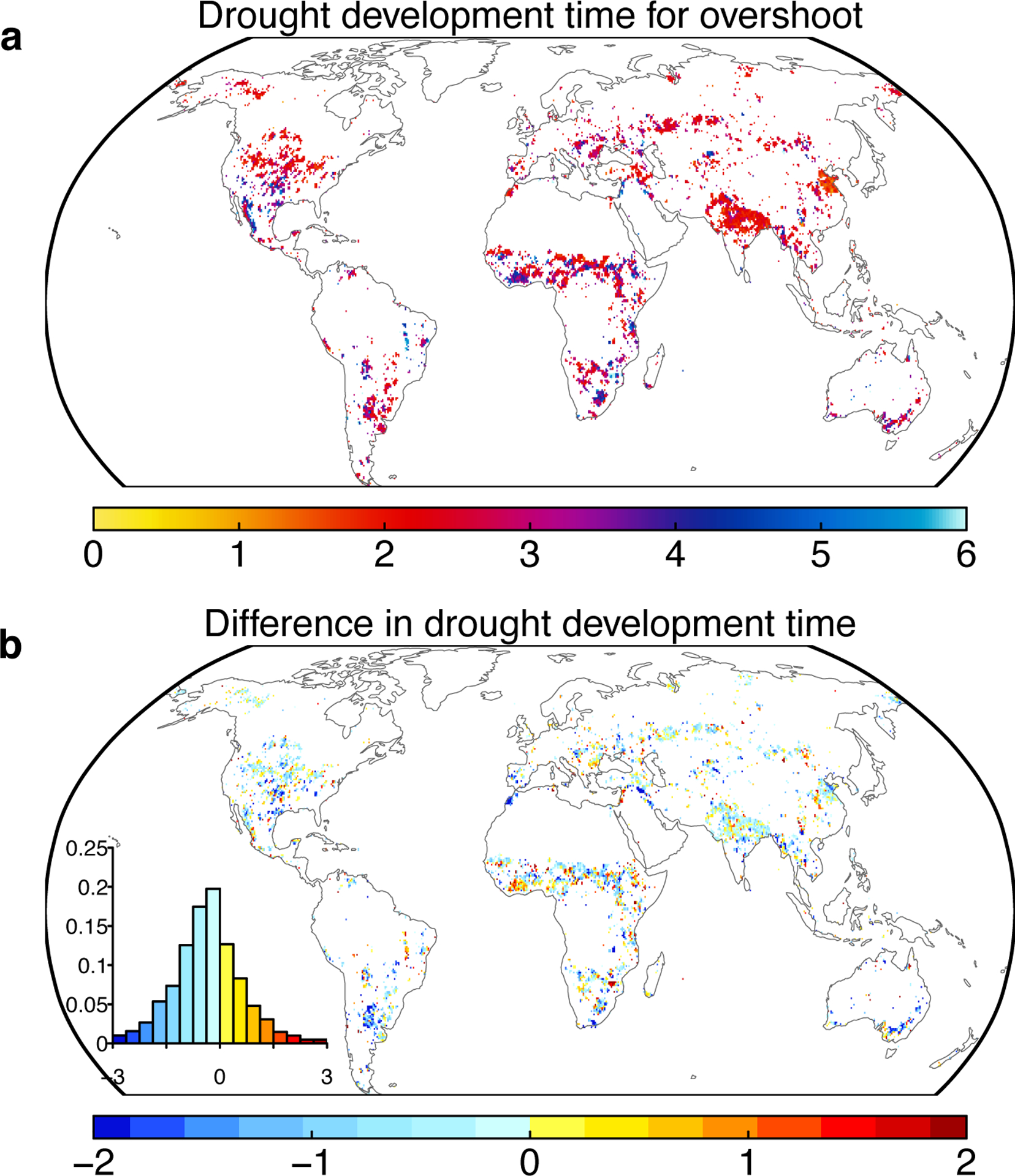
a average drought development time for overshoot drought event (in months). b Differences in drought development time between overshoot and non-overshoot droughts (in months). Drought development time is defined as the monotonical decrease period from local maximum to local minimum in the de-seasonalized detrended NDVI anomalies. Inset in b show the histogram of the differences.
Extended Data Fig. 9. Comparisons of drought severity and impact between overshoot and non-overshoot droughts.
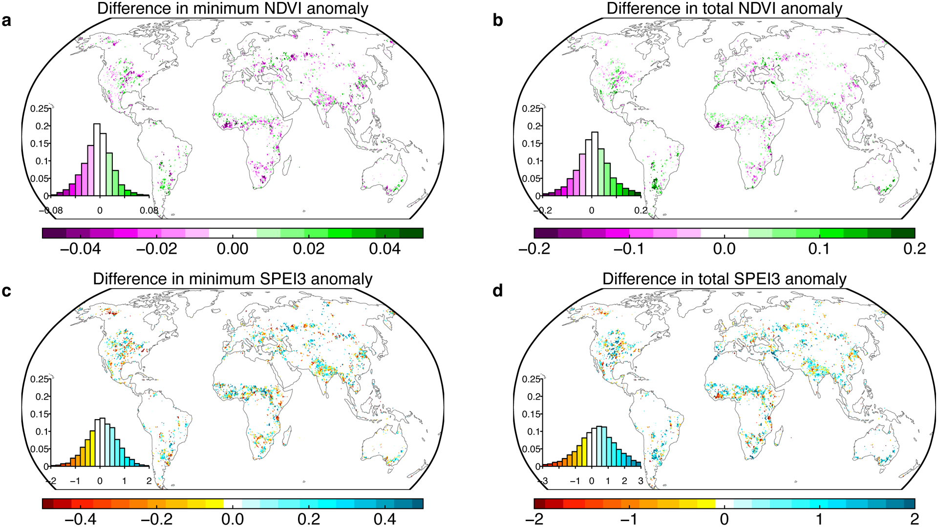
a Differences in minimum de-seasonalized detrended NDVI between overshoot and non-overshoot drought events. c Differences in minimum 3-month SPEI anomalies between overshoot and non-overshoot drought events. b and d, similar as a and c, but for differences of integrated sum of NDVI and SPEI during drought. Overshoot droughts, compared to the non-overshoot ones, usually have weaker drought stress (bottom panel), but relatively stronger impact on vegetation (upper panel). Insets show the histogram of differences in anomalies.
Extended Data Fig. 10. Comparison of the coefficients of the nested models that predict drought impact as a function of drought severity and overshoot occurrence.
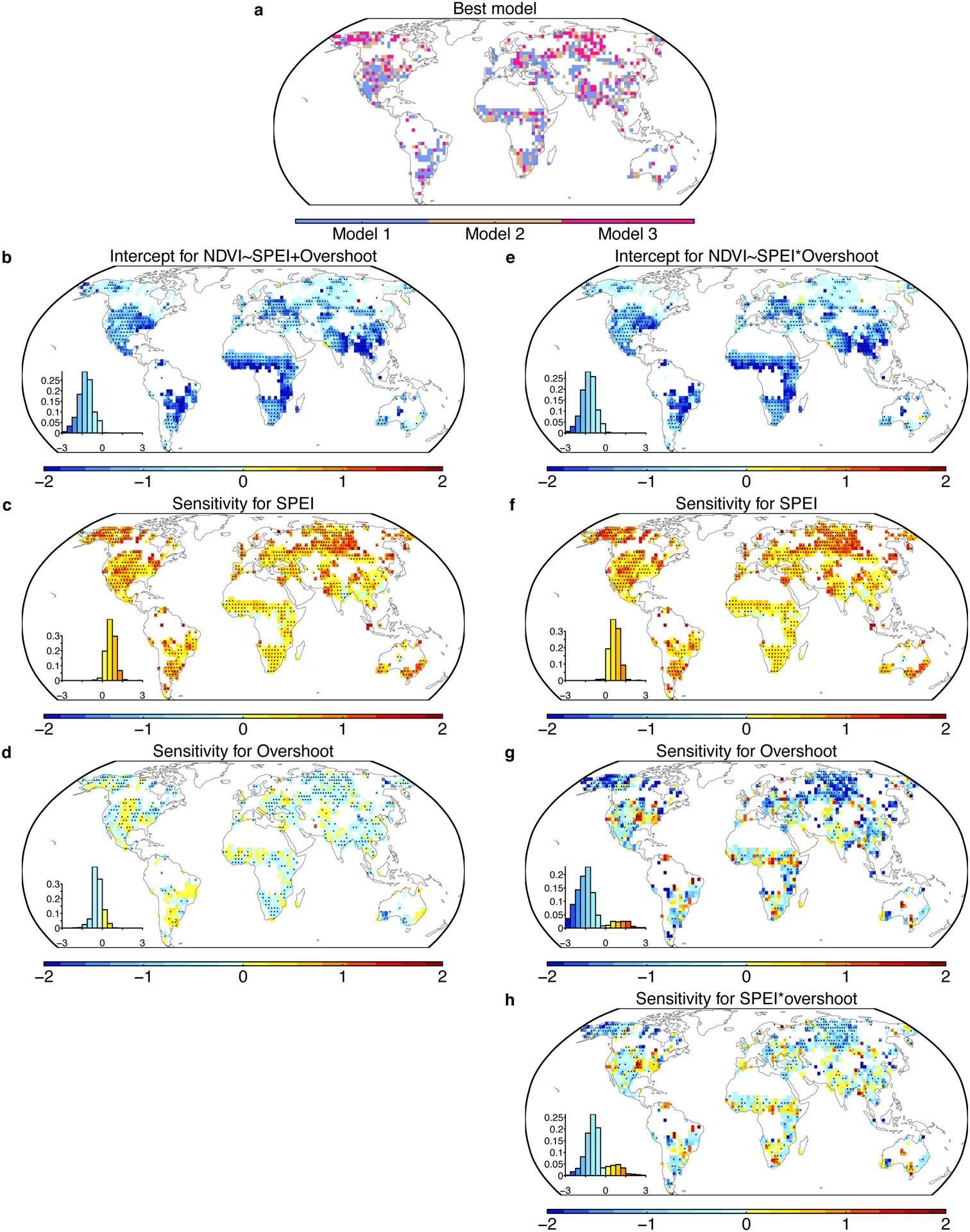
a spatial pattern of the best model being selected (see Methods). b-d coefficients for the model that overshoot only affects intercept. e-h coefficients for the model that overshoot affects both intercept and regression slope between NDVIz and SPEI. Insets show the histogram of the coefficients. Dotted areas indicate that the coefficient is significant at p<0.05.
Supplementary Material
Acknowledgements
YZ, TFK acknowledge support from the NASA IDS Award NNH17AE861. TFK acknowledges additional support from the US Department of Energy (DOE) under Contract DE-AC02-05CH11231 as part of the RuBiSCo SFA, a DOE Early Career Research Program award #DE-SC0021023, and an NSF PREEVENTS award #1854945. We thank Rene Orth for providing the SoMo.ml soil moisture data, and Vincent Humphrey for providing the GRACEτ data. We thank Yanlan Liu for discussion on the dynamic linear model method.
Footnotes
Competing Interests
The authors declare no competing interests.
References
- 1.Allen CD et al. A global overview of drought and heat-induced tree mortality reveals emerging climate change risks for forests. Forest Ecology and Management 259, 660–684 (2010). [Google Scholar]
- 2.Ciais P et al. Europe-wide reduction in primary productivity caused by the heat and drought in 2003. Nature 437, 529–533 (2005). [DOI] [PubMed] [Google Scholar]
- 3.Zhao M & Running SW Drought-Induced Reduction in Global Terrestrial Net Primary Production from 2000 Through 2009. Science 329, 940–943 (2010). [DOI] [PubMed] [Google Scholar]
- 4.Orth R & Destouni G Drought reduces blue-water fluxes more strongly than green-water fluxes in Europe. Nature Communications 9, 3602 (2018). [DOI] [PMC free article] [PubMed] [Google Scholar]
- 5.Doughty CE et al. Drought impact on forest carbon dynamics and fluxes in Amazonia. Nature 519, 78–82 (2015). [DOI] [PubMed] [Google Scholar]
- 6.Schwalm CR et al. Reduction in carbon uptake during turn of the century drought in western North America. Nature Geoscience 5, 551–556 (2012). [Google Scholar]
- 7.Bastos A et al. Direct and seasonal legacy effects of the 2018 heat wave and drought on European ecosystem productivity. Science Advances 6, eaba2724 (2020). [DOI] [PMC free article] [PubMed] [Google Scholar]
- 8.Wolf S et al. Warm spring reduced carbon cycle impact of the 2012 US summer drought. Proceedings of the National Academy of Sciences 113, 5880–5885 (2016). [DOI] [PMC free article] [PubMed] [Google Scholar]
- 9.Jump AS et al. Structural overshoot of tree growth with climate variability and the global spectrum of drought‐induced forest dieback. Global Change Biology 23, 3742–3757 (2017). [DOI] [PubMed] [Google Scholar]
- 10.Buermann W et al. Widespread seasonal compensation effects of spring warming on northern plant productivity. Nature 562, 110–114 (2018). [DOI] [PubMed] [Google Scholar]
- 11.Goulden ML & Bales RC California forest die-off linked to multi-year deep soil drying in 2012–2015 drought. Nat. Geosci 12, 632–637 (2019). [Google Scholar]
- 12.West M & Harrison J Bayesian forecasting and dynamic models. (Springer, 1997). [Google Scholar]
- 13.Pinzon JE & Tucker CJ A non-stationary 1981–2012 AVHRR NDVI3g time series. Remote Sensing 6, 6929–6960 (2014). [Google Scholar]
- 14.Nemani RR Climate-Driven Increases in Global Terrestrial Net Primary Production from 1982 to 1999. Science 300, 1560–1563 (2003). [DOI] [PubMed] [Google Scholar]
- 15.Zhang X, Friedl MA, Schaaf CB & Strahler AH Climate controls on vegetation phenological patterns in northern mid- and high latitudes inferred from MODIS data. Global Change Biology 10, 1133–1145 (2004). [Google Scholar]
- 16.Zeng Z et al. Impact of Earth Greening on the Terrestrial Water Cycle. J. Climate 31, 2633–2650 (2018). [Google Scholar]
- 17.Vicente-Serrano SM et al. Response of vegetation to drought time-scales across global land biomes. Proceedings of the National Academy of Sciences 110, 52–57 (2013). [DOI] [PMC free article] [PubMed] [Google Scholar]
- 18.Anderegg WRL et al. Hydraulic diversity of forests regulates ecosystem resilience during drought. Nature 561, 538–541 (2018). [DOI] [PubMed] [Google Scholar]
- 19.Isbell F et al. Biodiversity increases the resistance of ecosystem productivity to climate extremes. Nature 526, 574–577 (2015). [DOI] [PubMed] [Google Scholar]
- 20.Lian X et al. Partitioning global land evapotranspiration using CMIP5 models constrained by observations. Nature Climate Change 8, 640–646 (2018). [Google Scholar]
- 21.Zscheischler J et al. Future climate risk from compound events. Nature Clim Change 8, 469–477 (2018). [Google Scholar]
- 22.Zscheischler J et al. A typology of compound weather and climate events. Nat Rev Earth Environ 1, 333–347 (2020). [Google Scholar]
- 23.Zhou S, Zhang Y, Williams AP & Gentine P Projected increases in intensity, frequency, and terrestrial carbon costs of compound drought and aridity events. Science Advances 5, eaau5740 (2019). [DOI] [PMC free article] [PubMed] [Google Scholar]
- 24.Hersbach H et al. The ERA5 global reanalysis. Q.J.R. Meteorol. Soc 146, 1999–2049 (2020). [Google Scholar]
- 25.O S & Orth R Global soil moisture data derived through machine learning trained with in-situ measurements. Sci Data 8, 170 (2021). [DOI] [PMC free article] [PubMed] [Google Scholar]
- 26.Pendergrass AG et al. Flash droughts present a new challenge for subseasonal-to-seasonal prediction. Nature Climate Change 10, 191–199 (2020). [Google Scholar]
- 27.Otkin JA et al. Flash Droughts: A Review and Assessment of the Challenges Imposed by Rapid-Onset Droughts in the United States. Bulletin of the American Meteorological Society 99, 911–919 (2018). [Google Scholar]
- 28.Lian X et al. Summer soil drying exacerbated by earlier spring greening of northern vegetation. Science Advances 6, eaax0255 (2020). [DOI] [PMC free article] [PubMed] [Google Scholar]
- 29.Green JK et al. Regionally strong feedbacks between the atmosphere and terrestrial biosphere. Nature Geoscience 10, 410–414 (2017). [DOI] [PMC free article] [PubMed] [Google Scholar]
- 30.Keenan TF & Richardson AD The timing of autumn senescence is affected by the timing of spring phenology: implications for predictive models. Global Change Biology 21, 2634–2641 (2015). [DOI] [PubMed] [Google Scholar]
- 31.Zani D, Crowther TW, Mo L, Renner SS & Zohner CM Increased growing-season productivity drives earlier autumn leaf senescence in temperate trees. Science 7 (2020). [DOI] [PubMed] [Google Scholar]
- 32.Buitenwerf R, Rose L & Higgins SI Three decades of multi-dimensional change in global leaf phenology. Nature Climate Change 5, 364–368 (2015). [Google Scholar]
- 33.Douville H, Ribes A, Decharme B, Alkama R & Sheffield J Anthropogenic influence on multidecadal changes in reconstructed global evapotranspiration. Nature Climate Change 3, 59–62 (2013). [Google Scholar]
- 34.Asrar G, Fuchs M, Kanemasu ET & Hatfield JL Estimating Absorbed Photosynthetic Radiation and Leaf Area Index from Spectral Reflectance in Wheat. Agronomy Journal 76, 300–306 (1984). [Google Scholar]
- 35.Chen JM & Cihlar J Retrieving leaf area index of boreal conifer forests using Landsat TM images. Remote Sensing of Environment 55, 153–162 (1996). [Google Scholar]
- 36.Piao S et al. Characteristics, drivers and feedbacks of global greening. Nature Reviews Earth & Environment 1, 14–27 (2020). [Google Scholar]
- 37.Becker A et al. A description of the global land-surface precipitation data products of the Global Precipitation Climatology Centre with sample applications including centennial (trend) analysis from 1901–present. Earth System Science Data 5, 71–99 (2013). [Google Scholar]
- 38.Harris I, Osborn TJ, Jones P & Lister D Version 4 of the CRU TS monthly high-resolution gridded multivariate climate dataset. Scientific Data 7, (2020). [DOI] [PMC free article] [PubMed] [Google Scholar]
- 39.Sun Q et al. A Review of Global Precipitation Data Sets: Data Sources, Estimation, and Intercomparisons. Rev. Geophys 56, 79–107 (2018). [Google Scholar]
- 40.Vicente-Serrano SM, Beguería S & López-Moreno JI A Multiscalar Drought Index Sensitive to Global Warming: The Standardized Precipitation Evapotranspiration Index. Journal of Climate 23, 1696–1718 (2010). [Google Scholar]
- 41.Harrison PJ & Stevens CF Bayesian Forecasting. Journal of the Royal Statistical Society. Series B (Methodological) 38, 205–247 (1976). [Google Scholar]
- 42.Liu Y, Kumar M, Katul GG & Porporato A Reduced resilience as an early warning signal of forest mortality. Nat. Clim. Chang 9, 880–885 (2019). [Google Scholar]
- 43.Humphrey V, Gudmundsson L & Seneviratne SI Assessing Global Water Storage Variability from GRACE: Trends, Seasonal Cycle, Subseasonal Anomalies and Extremes. Surv Geophys 37, 357–395 (2016). [DOI] [PMC free article] [PubMed] [Google Scholar]
- 44.Schwalm CR et al. Global patterns of drought recovery. Nature 548, 202–205 (2017). [DOI] [PubMed] [Google Scholar]
Associated Data
This section collects any data citations, data availability statements, or supplementary materials included in this article.
Supplementary Materials
Data Availability Statement
The NDVI 3g v1 dataset is available at https://ecocast.arc.nasa.gov/data/pub/gimms/, the CRU climate dataset is available at https://crudata.uea.ac.uk/cru/data/hrg/, the GPCC precipitation data is available at https://www.dwd.de/EN/ourservices/gpcc/gpcc.html, phenology metrics derived from MODIS are available at https://vip.arizona.edu/viplab_data_explorer.php, the SPEI dataset is available at https://spei.csic.es/database.htmlt, the ERA5 soil moisture data is available at https://cds.climate.copernicus.eu/cdsapp#!/dataset/reanalysis-era5-land-monthly-means, the SoMo.ml soil moisture data is from https://www.bgc-jena.mpg.de/geodb/projects/Home.php. The source data for the figures are publicly available (https://doi.org/10.6084/m9.figshare.15086535)


