

Summary
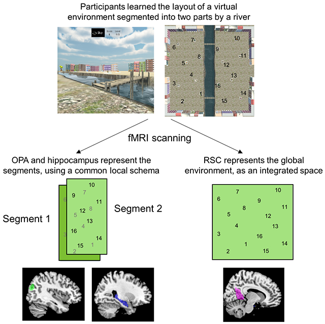
Humans and animals use cognitive maps to represent the spatial structure of the environment. Although these maps are typically conceptualized as extending in an equipotential manner across known space, behavioral evidence suggests that people mentally segment complex environments into subspaces. To understand the neurocognitive mechanisms behind this operation, we familiarized participants with a virtual courtyard that was divided into two halves by a river; we then used behavioral testing and fMRI to understand how spatial locations were encoded within this environment. Participants’ spatial judgments and multivoxel activation patterns were affected by the division of the courtyard, indicating that the presence of a boundary can induce mental segmentation even when all parts of the environment are co-visible. In the hippocampus and occipital place area (OPA), the segmented organization of the environment manifested in schematic spatial codes that represented geometrically-equivalent locations in the two subspaces as similar. In the retrosplenial complex (RSC), responses were more consistent with an integrated spatial map. These results demonstrate that people use both local spatial schemas and integrated spatial maps to represent segmented environment. We hypothesize that schematization may serve as a general mechanism for organizing complex knowledge structures in terms of their component elements.
Keywords: RSC, OPA, hippocampus, fMRI, cognitive map, spatial memory, scene perception
eTOC
Navigable environments can often be segmented into subspaces or regions. Peer and Epstein show that when people learn a virtual environment containing multiple subspaces, OPA and hippocampus encode local maps that reflect the common geometric structure of the subspaces. These spatial schemas may be a key component of cognitive maps.
Graphical Abstract
Introduction
To navigate in space, humans and animals form cognitive maps of their environment. In the classical formulation, these maps are Euclidean reference frames that extend across space in a global and equipotential manner1. In contrast, alternative models suggest that cognitive maps are segmented into multiple local representations, which are then organized into a hierarchy or graph2–8. Consistent with the latter view, psychological studies have reported effects of segmentation on spatial memory, spatial priming, navigational strategies, and episodic memory9–13. Segmentation effects are also observed in the temporal domain, where the mind/brain appears to divide experience into discrete events14–16. Thus, segmentation might be a general principle by which the mind-brain organizes both spatial and nonspatial information. However, the neural underpinnings of mental segmentation are not well understood6,17.
Some insight into this issue comes from studies that have examined neural representations in environments with multiple subspaces. When rodents explore mazes with several connected compartments, place and grid cells in the hippocampal formation can distinguish the compartments in several ways18,19. First, by repeating the same firing fields in geometrically equivalent locations in different compartments, a phenomenon we refer to as schematization because it suggests the use of a spatial schema that applies across different subspaces20–24. Second, by forming distinct representations of each compartment22,25, a phenomenon known as remapping22,26,27. Human fMRI studies have found evidence for schematization in hippocampus28, entorhinal cortex29 and the retrosplenial/medial parietal cortex30 when participants are tested on environments with connected subspaces, and evidence for remapping in hippocampus when participants are tested on unconnected environments31,32. In addition, a third possible mechanism for spatial segmentation was observed in a recent study that found representational discontinuities across texture boundaries in hippocampal place cells33. Under this phenomenon, which we call grouping, items within the same subspace are representationally more similar than items in different subspaces. In humans, grouping been observed in the hippocampus and prefrontal cortex when people view temporal sequences of items34,35 or watch movies15.
Human psychological work has observed behavioral patterns that are consistent with schematization36 and grouping3,10,37–43. However, interpretation of these results—and also previous neural findings—is complicated by the fact that most previous studies used environments in which subspaces were defined by boundaries that restricted the view between segments37,38,40,44 and constrained participants’ movements such that they tended to spend time in each subspace before moving to the next one45,46. Therefore, many previously observed segmentation effects could be a byproduct of the brain’s proclivity to organize memories by shared perceptual context14,47 or temporal and probabilistic contiguity16,34,48. However, some behavioral findings indicate that segmentation effects can occur without walls, e.g. between shopping and business districts of a city9,10,13, suggesting that segmentation into subspaces can be induced in a top-down manner, based on spatial or conceptual organization.
In the current experiment, we aimed to identify the neural mechanisms behind such top-down spatial segmentation, with the specific goal of determining if behavioral segmentation effects are accompanied by neural effects of schematization, grouping or remapping. We trained participants to locate 16 objects in a segmented environment for which visibility, spatial relations and the probability of transition between objects were matched within and between segments. We then used fMRI to identify object-specific activity patterns, and we investigated how these neural representations were affected by the spatial segmentation. To anticipate, we observed behavioral and neural effects of segmentation; the neural effects were observed in the hippocampus and scene-selective regions of the visual system, and they manifested primarily as schematization.
Results
Division of the environment into subspaces induces mental segmentation
To encourage the formation of segmented spatial representations, we familiarized participants with a virtual courtyard that was divided into two segments by a river crossable at two bridges (Fig. 1). The river blocked movement (except at the bridges), but it did not block visibility. Participants learned the locations of 16 objects within the courtyard through a multi-stage learning procedure in which they were required to navigate to named objects in succession. The order of these navigational targets was randomized so that that participants’ navigational paths were not related to the proximity of the objects or the division of the environment into subspaces. Initially all objects were visible, but as training progressed, increasing numbers of the objects were obscured to induce reliance on spatial memory (see Experimental Procedures). By the end of the learning procedure, all of the participants included in the experiment could navigate to all object locations without error, even when all the objects were obscured (Fig. S1A). The learning stage took 28 minutes on average (range: 16-51 minutes).
Figure 1: Experimental design and procedure.
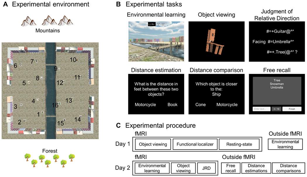
A) Participants were familiarized with a virtual environment consisting of a square courtyard surrounded by buildings. A river separated the environment into two segments and two bridges allowed crossing from one segment to the other. Sixteen objects were located in the environment, with their locations balanced such that distances and directions between objects were similar within each segment and between segments (e.g. objects 1 and 5, 5 and 9, 9 and 13, 13 and 1 are equally distant from each other). B) Experimental tasks. C) Experimental procedure. Note that the object viewing and judgment of relative direction tasks were performed in the fMRI scanner, while the free recall, distance estimation, and distance comparison tasks were performed outside the scanner. For full details on the tasks and procedure, see STAR Methods.
Behavioral assessments confirmed that participants formed segmented spatial representations that reflected the division of the courtyard into two subspaces (Fig. 2). When participants were asked to estimate distances between objects (distance estimation task), their responses were significantly more accurate for object pairs on same side of the river compared to object pairs on opposite sides of the river (correlation between real and estimated distances – r=0.72 within segment; r=0.60 between segment; difference – Z=2.32, p=0.02, effect size r=0.47; Fig. 2A left). Similarly, when participants were asked to make three-way distance comparisons between objects (distance comparison task, e.g. “which object is closer to object A: object B or object C?”), they made more correct responses when all three objects were on the same side of the river compared to when the anchor and target objects were on opposite sides (average accuracy=86% within segment; 77% between segment; difference – Z=2.87, p=0.004, effect size r=0.59; Fig. 2A right). For both distance tasks, trials were constructed so that average Euclidean distance was equal for within-segment and between-segment conditions. Results were similar when data were analyzed using shortest path distance instead of Euclidean distance as the ground truth (within-segment vs. between-segments accuracy: Z=3.23, p=0.001, effect size r=0.66 for distance estimations; Z=2.93, p=0.003, effect size r=0.60 for distance comparisons; note that Euclidean and path distances were highly correlated to each other, when considering either all distances [r=0.92] or only the between-segment distances [r=0.86]).
Figure 2: Behavioral evidence for segmented spatial representations.
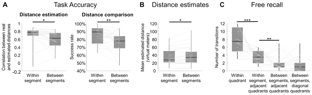
A) In the distance estimation and distance comparison tasks, performance was higher for within-segment judgments than between-segment judgments, demonstrating that within-segment spatial relationships were more accurately represented. B) In the distance estimation task, estimates were larger for between-segment distances than within-segment distances, even though the true distances were matched across these two conditions. C) In the free recall task, consecutive recall of objects within the same quadrant was the most common, demonstrating an effect of spatial proximity. In addition, sequential recall of objects in the adjacent quadrant of the same segment was more frequent than sequential recall of objects in the adjacent quadrant in the other segment, demonstrating an effect of segmentation. Box plot whiskers indicate minimum to maximum values, horizontal lines inside boxes indicate medians across participants, and boxes indicate values between the upper and lower data quartiles. Asterisks represent significant differences (p<0.05, two-tailed Wilcoxon signed-rank tests across participants). See Fig. S1 for additional behavioral results.
Further analyses of the data from the distance estimation task revealed that participants estimated distances as being larger for between-segment compared to within-segment object pairs, even though the actual distances were matched between these conditions (Z=2.01, p=0.047, effect size r=0.41; Fig. 2B). Analysis of reaction times did not reveal any segment-related priming in the distance estimation task, which was not surprising given the unspeeded nature of the required response. In the distance comparison task, however, we did observe priming: responses on within-segment triads preceded by another within-segment triad were faster if both triads were on the same side of the river (Z=3.0, p=0.003, effect size r=0.61). Overall, these results support the idea that the segments have some degree of representational distinction, which manifests as distortions in the accuracy and magnitude of distance representations, and also as behavioral priming.
Segmentation effects were also observed in the free recall task. Participants in this task were asked to name the objects in any order (Fig. 2C). All participants recalled all 16 object names except for one participant who recalled 15 names. The order of spatial recall was shaped by spatial proximity and by the division into subspaces. Objects were significantly more likely to be remembered in sequence if they were close to each other in the environment (average spatial distance between consecutively-recalled objects / average distance between objects if chosen randomly = 0.70, Z=4.26, p<0.0001, effect size r=0.87)49. In addition, sequential recall of objects from the same segment was more likely than sequential recall of objects from different segments (considering only adjacent-quadrant object pairs to control for distance; Z=2.72, p=0.007, effect size r=0.55; Fig. 2C).
Finally, when participants were asked to report the size of the environment along each direction, 74% gave different values for the length and width, indicating that they remembered the courtyard as being rectangular when in fact it was a perfect square (Fig. S1B).
Multivoxel patterns contain information about the spatial locations of objects
We then turned towards the main question of the study: how is the spatial structure of the segmented courtyard encoded in the brain? To this end, we scanned participants with fMRI while they performed two tasks that were designed to activate mnemonic representations of the environment (i.e. cognitive maps). On each trial of the judgment of relative direction (JRD) task, participants imagined themselves standing at one object (starting object) while facing a second object (facing object) and indicated whether a third object (target object) would be on their left or right from the imagined point of view. On each trial of the object viewing task, participants viewed an image of a single object shown outside of any spatial context and indicated if it was in an upright or slightly tilted orientation. These tasks allowed us to probe neural responses related to the spatial locations of the 16 objects, but in different ways: in the JRD task, participants explicitly retrieved spatial information from memory, whereas in the object viewing task, they implicitly retrieved spatial information embedded in object representations. Previous work has shown that spatial codes in RSC are most often observed during explicit tasks30,50–53 while spatial codes in hippocampus are most often observed in implicit tasks54–57. We included both tasks to get a full picture of how spatial representations are affected by segmentation.
We used representational similarity analysis to investigate the spatial codes elicited during each task. Representational similarity matrices (RSMs) were constructed based on multivoxel activity patterns elicited by the 16 objects. These neural RSMs were then compared to model RSMs, which were constructed to reflect the predicted similarities between the objects under different spatial coding schemes. Our analyses focused on five regions of interest (ROIs) that have been previously implicated in the coding of spatial scenes and cognitive maps: retrosplenial complex (RSC), parahippocampal place area (PPA), occipital place area (OPA), hippocampus, and entorhinal cortex (ERC). To obtain voxels involved in task-related mnemonic recall58, RSC, PPA and OPA were defined by selecting the most active voxels for each task within a pre-defined search space (see Fig. S2 for comparison to ROIs defined using a scene perception localizer). The hippocampus and ERC were defined anatomically (Fig. S2). In this section, we report analyses of the data in terms of the veridical Euclidean distances between the objects, as a first pass method for identifying map-like spatial codes. We refer to this model as the integration model, because it assumes full integration between all parts of the environment, irrespective of the division into subspaces.
Participants performed the JRD task at above-chance level (percent correct answers – 68%, Z=3.72, p=0.0002, effect size r=0.76) but accuracy did not depend on whether the starting, facing, and target objects were all in the same segment or not (within-segment vs. between-segment comparison: Z=0.1, p=0.92, effect size r=0.02). For each ROI, we calculated RSMs based on the starting objects on each trial, as these objects indicated the imagined location of the participant. Comparison of these neural RSMs to the Euclidean distance RSM (Fig. 3) revealed coding of inter-object distances in RSC (Z=2.81, p=0.012, effect size r=0.59) and OPA (Z=2.37, p=0.021, effect size r=0.49), with a marginal trend in PPA (Z=1.64, p=0.086, effect size r=0.34; all p-values FDR-corrected for multiple comparisons across ROIs). There were no significant effects in hippocampus or ERC (all Zs≤0.72, all ps≥0.29).
Figure 3: fMRI activity patterns contain information about distances between objects.
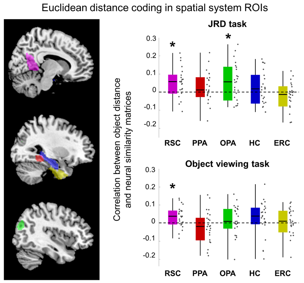
Left panel shows the anatomical extent of hippocampus and ERC, and the parcels used to define RSC, PPA, and OPA. Right panel shows results of representational similarity analyses. For each region of interest (ROI), a neural similarity matrix was calculated based on multivoxel patterns elicited by the 16 objects, separately for the judgment of relative direction (JRD) and object viewing tasks. These neural matrices were compared to a model similarity matrix based on the veridical Euclidean (i.e. straight-line) distances between objects. Significant coding of distances between objects was found in RSC and OPA (asterisks indicate p-values < 0.05, one-sample Wilcoxon signed-rank test across participants, FDR-corrected for multiple comparisons across ROIs). Distance coding effects in PPA in the JRD task and in hippocampus in the object viewing task were close to significance (p=0.086 and p=0.096, respectively). RSC – retrosplenial complex, PPA – parahippocampal place area, OPA – occipital place area, HC – hippocampus, ERC – entorhinal cortex. Dots indicate individual data points. Box plot elements are the same as in Figure 2.
The object viewing task was administered twice: once before participants were familiarized with the virtual environment (day 1), and once again after environmental learning (day 2). Performance on both days was near ceiling (average accuracy – 94%, Z=4.3, p=0.00002, effect size r=0.88). On day 2, we observed spatial priming: response times on each trial were correlated with the distance between the observed object and the object shown on the preceding trial (average correlation r=0.03, Z=2.69, p=0.007, effect size r=0.55); this effect was not observed on day 1 (Z=1.1, p=0.26, effect size r=0.22). However, we did not observe day 2 priming related to the consecutive presentation of objects from the same segment (Z=1.07, p=0.28, effect size r=0.21). To investigate the spatial codes induced in the brain by environmental learning, we calculated neural RSMs based on the multivoxel patterns elicited by each object on day 1 and day 2 and then calculated the difference between these two matrices. This approach minimizes the contribution of non-learning related factors that may affect the similarity between neural patterns (e.g. semantic or perceptual similarity)56. Comparison of this neural pattern difference matrix to the Euclidean distance RSM revealed significant Euclidean distance coding in RSC (Z=2.61, p=0.02, effect size r=0.53), and a marginal trend in hippocampus (Z=1.77, p=0.096, effect size r=0.36), but not in any other ROI (all ps>0.19).
Schematization effects are observed in scene-selective areas and the hippocampus
We next tested the fMRI responses in each ROI for evidence of three possible spatial segmentation effects: schematization, grouping, and remapping. Figure 4 shows the results of these analysis in ROIs exhibiting significant effects, and Figure S3 shows the results for all ROIs.
Figure 4: fMRI evidence for schematic and integrated representation of spatial segments.
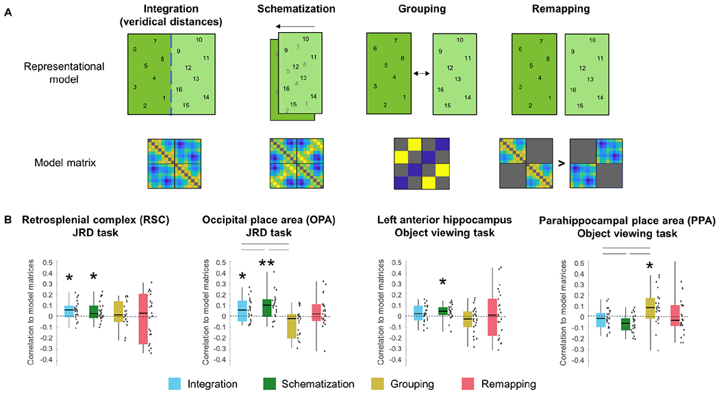
A) Top row graphically depicts four different models of spatial coding, with numbers indicating the locations of the 16 objects within the putative representational space; second row shows the corresponding representational similarity matrices (See text for details; note that the Integration Model is the same as the Euclidean distance model plotted in Fig. 3.) B) Significant correlations between model matrices and neural pattern similarity matrices were observed in RSC, OPA, left anterior hippocampus and PPA (see Fig. S3 for results in all ROIs). The integration and schematization models predict neural pattern similarities in RSC and OPA during the JRD task, while the schematization model predicts neural pattern similarity in left anterior hippocampus during the object viewing task. The grouping model predicted neural similarities in the PPA during the object viewing task, although this effect was not replicated using a different grouping measure (see Results). The remapping model did not predict neural similarities in any ROI. Asterisks denote significant effects (* p<0.05; ** p<0.01; One-tailed one-sample Wilcoxon signed-rank test for each model in each ROI, p-values for each task and model are FDR-corrected for multiple comparisons across ROIs). RSC – retrosplenial complex, PPA – parahippocampal place area, OPA – occipital place area. Lines represent significant differences between models (Wilcoxon signed-rank pairwise tests, FDR-corrected for comparisons between the integration, schematization and grouping models). Dots indicate individual data points. Box plot elements are the same as in Figure 2. See Fig. S4 for exploration of different schematization models.
Under the schematization scenario, locations are coded with respect to the geometry of each segment, but in a manner that generalizes across segments. In the current environment, schematization can be conceptualized as overlaying the two segments onto a single common space, such that (for example) an object in the “Northeast” corner of one segment will be assigned the same spatial coordinates as an object in the “Northeast” corner of the other segment. To test for these effects, we created a model RSM under the assumption of overlay and compared to neural pattern similarities in each ROI (see Fig. S4 for exploration of other possible schematization models). In the JRD task, we observed significant schematization effects in RSC (Z=2.27, p=0.029, effect size r=0.47) and OPA (Z=3.39, p=0.002, effect size r=0.71), but not in PPA, hippocampus or entorhinal cortex (all Zs≤0.07, all ps≥0.66; Figs. 4, S3). In the object viewing task, we observed a schematization effect in hippocampus (Z=2.38, p=0.046, effect size r=0.49) but not in the other four ROIs (all Zs≤1.5, all ps≥0.2; Fig. S3).
Analysis of effects in each hemisphere separately demonstrated that schematization occurred in left RSC and left OPA during the JRD task (although the effect was close to significance in right OPA), and in left hippocampus during the object viewing task (Fig. S3). For the hippocampus, we further divided each hemisphere into anterior and posterior portions, in light of previous studies that have found spatial codes that are restricted to the left anterior subregion28,54,55. Consistent with these earlier results, the schematization effect during the object viewing task was significant in left anterior hippocampus (Z=2.99, p=0.01, effect size r=0.61; Fig. 4D) but not in the other three hippocampal subregions (all Zs≤0.1.2, all ps≥0.2, FDR-corrected across all ROIs including the four hippocampal subregions).
Under the grouping scenario, within-segment distances are compressed compared to between-segment distances, over and beyond what would be expected based on Euclidean distance. To measure grouping, we calculated the average neural similarity for within-segment and between-segment object pairs and compared these two values, using only distances between objects in adjacent quadrants to control for Euclidean distance. No significant grouping effect was found in any ROI in the JRD task (all Zs≤1, all ps≥0.3). In the object-viewing task, a significant grouping effect was found in the PPA (Z=2.53, p=0.021, effect size r=0.54), but not in other ROIs (all Zs≤0.8, all ps≥0.5; Fig. 4). We also examined a different measure of grouping that takes into account the distances between all the objects, including objects in the same quadrant and non-adjacent quadrants (see STAR Methods); this measure found no significant grouping effects in any ROI, including the PPA (all Zs<1.1, all ps>0.48). Therefore, grouping might be present in the PPA, but this finding is inconclusive.
Under the remapping scenario, the two segments should have distinct spatial representations, which would be independent of each other in the case of complete remapping. Thus, neural distances within each segment should reflect distances in the virtual world, whereas neural distances across segments should not. Following this logic, we indexed remapping by calculating the average correlation between neural distances and Euclidean distances, separately for within-segment and between-segment object pairs, and taking the difference between these two values. We did not find evidence for remapping in any ROI in either the JRD task (all Zs≤1.8, all ps≥0.1) or in the object viewing task (all Zs≤1.4, all ps≥0.4; Fig. 4).
Thus, we found evidence for both schematization and integration in OPA and RSC during the JRD task, and evidence for schematization in left anterior hippocampus and grouping in the PPA during the object viewing task (although the PPA finding was inconclusive). The OPA and RSC findings were further supported by results from a previous study that examined object codes in a multi-chamber environment during a JRD task30; a re-analysis of these data found evidence for integration and schematization in both regions (Fig. S5). We did not find evidence for remapping in any region (although see Discussion).
The schematization and integration models are correlated to each other (r=0.63; this can be easily seen by considering the fact the dimension along the river is the same in both models). Thus, it is not surprising that both models fit the neural data in OPA and RSC. To compare these models, we used two approaches. First, we used two-tailed paired-sample Wilcoxon signed-rank tests to compare correlation values between the schematization and integration models. For completeness, we also included the grouping model in this analysis, because it was also indexed by a correlation value. In OPA, the schematization model provided a better fit to the neural RDM than the integration model (Z=2.28, p=0.02, effect size r=0.48) or the grouping model (Z=2.28, p=0.02, effect size r=0.48). The fits of the three models did not differ in RSC (all Zs<1.07, all ps>0.64) or left anterior hippocampus (all Zs<0.86, all ps>0.67; results FDR-corrected within each ROI for all comparisons across the integration, schematization and grouping models). Second, we used partial correlation to determine if the schematization models remained significant when regressing out the variance explained by the integration model, and vice versa. In OPA and left anterior hippocampus, the schematization model remained significant when accounting for the variance of the integration model (Z=3.15,2.07, p=0.0008,0.02, effect size r=0.66,0.43, respectively), but the integration model did not remain significant when accounting for the variance of the schematization model (p=0.57,0.36, respectively). In RSC, by contrast, the integration model remained significant when controlling for the schematization model (Z=1.75, p=0.04, effect size r=0.36), but the schematization model did not remain significant when controlling for the integration model (p=0.27). These results suggest that responses in OPA and left anterior hippocampus are best explained by the schematization model, whereas responses in RSC are best explained by the integration model.
Searchlight analyses confirm schematization and integration effects
To investigate spatial coding outside of the ROIs, we performed whole-brain searchlight analyses of integration, schematization, grouping and remapping. No effects survived correction for multiple comparisons across the entire brain, but when analyses were restricted to a search space encompassing the five ROIs (hippocampus, entorhinal cortex, and the parcels used to define PPA, RSC, and OPA), right RSC demonstrated significant correlation to the integration and schematization models in the JRD task (Fig. 5A–B). No significant effects were observed in OPA, possibly due to the small size of this parcel. We also performed an exploratory searchlight analysis using the medial temporal lobe (hippocampus and entorhinal cortex) as an anatomical mask, due to the importance of this region in spatial representation. This analysis identified a significant schematization effect in left anterior hippocampus in the object viewing task (Fig. 5C), consistent with the results from the analysis of hippocampal subregions. No other models were significant in any region. These results corroborate the ROI findings of schematization and integration effects in RSC and schematization effects in left anterior hippocampus.
Figure 5: Searchlight analysis reveals integration and schematization effects.
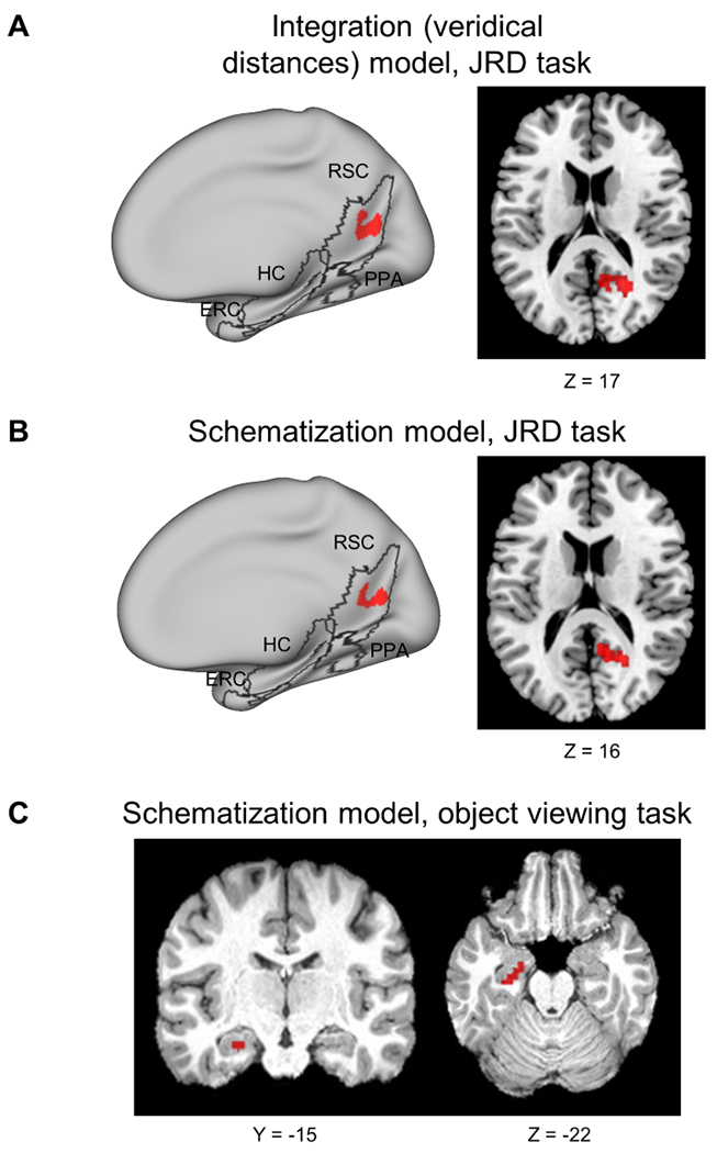
A) Integration (veridical Euclidean distance) model predicts fMRI pattern similarity in RSC during the JRD task (291 significant voxels; searchlight constrained to all-ROIs mask). B) Schematization model predicts fMRI pattern similarity in RSC during JRD task (221 significant voxels; searchlight constrained to all-ROIs mask). C) Schematization model predicts fMRI pattern similarity in left anterior hippocampus during the object-viewing task data (55 significant voxels; searchlight constrained to bilateral hippocampus and entorhinal cortex). Red – significant clusters, Monte-Carlo permutation testing, TFCE corrected for multiple comparisons, p<0.05. ROI outlines (RSC, PPA, OPA, HC, EC) are marked in black. RSC – retrosplenial complex, PPA – parahippocampal place area, OPA – occipital place area, HC – hippocampus, ERC – entorhinal cortex.
Visualization of schematization effects through multidimensional scaling of neural patterns
To provide a visualization of how schematization manifests in neural similarity space, we performed multidimensional scaling (MDS) on the pattern similarity matrices from OPA, RSC, and left anterior hippocampus. The results in OPA were consistent with the use of a single spatial representation that is overlaid onto to both subspaces (Fig. 6). Objects from the two segments were representationally interdigitated, but objects were separable along the spatial dimension parallel to the river (“North” vs. “South”), which is common to both segments. Moreover, objects were separable along the dimension perpendicular to the river (“East” vs. “West”) when this dimension was put into a common local space by considering it within each segment. These results illustrate that objects are represented in OPA according to their location relative to the geometric structure that is common to both segments. The MDS results in RSC (Fig. S6, top) were most easily interpreted in terms of the integrative model, and MDS results in left anterior hippocampus (Fig. S6, bottom) were not easily interpretable though there was some evidence for separation of objects along the North/South axis.
Figure 6: Visualization of the schematization in the occipital place area (OPA) using multidimensional scaling of fMRI pattern similarities.
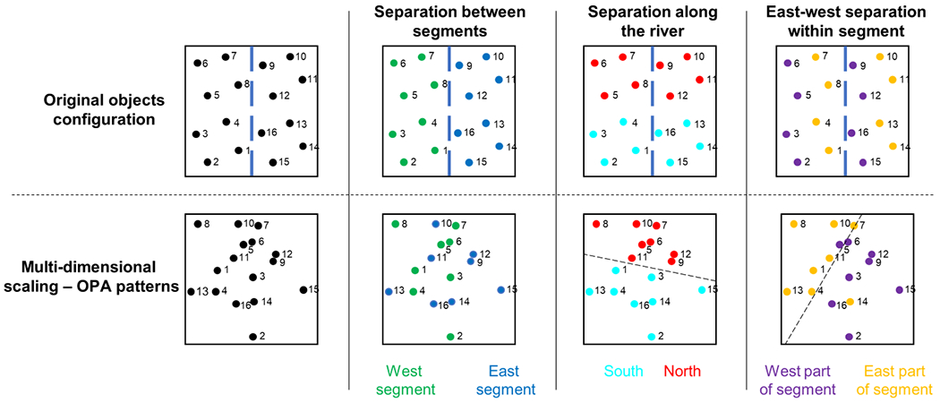
Top row shows the true configuration of the objects in the environment; bottom row shows the results of multidimensional scaling of activity patterns in OPA, from the JRD task data. OPA does not distinguish between objects in different segments (second column), but it does distinguish between objects in the upper (“north”) and lower (“south”) parts of the environment (third column), and between objects in the left (“west”) and right (“east”) parts of each segment (fourth column). These findings suggest that OPA represents the subspaces as overlaid on each other, such that the common North/South axis is preserved, and East/West is represented within but not across segments. Dashed blue line in top row indicates the location of the river; dashed black lines in bottom row illustrate the separability of neural patterns. See Fig. S6 for multidimensional scaling results in RSC and hippocampus.
Discussion
The principal goal of this study was to understand how the human brain represents the segmented structure of complex spatial environments. We familiarized participants with a virtual courtyard that was divided into two halves by a river, and we assessed their representations of this environment using behavioral testing and fMRI. We found that the division of the environment into subspaces affected participants’ distance judgments, free recall order, and sketch maps. Crucially, segmentation effects were also observed in fMRI signals. Multivoxel activation patterns in the medial temporal lobe (hippocampus) and scene regions (RSC and OPA) contained information about the distances between objects, but these distance codes were distorted from Euclidean ground-truth by the subspace organization. In hippocampus and OPA, objects in geometrically similar locations across subspaces elicited similar activation patterns, consistent with the use of local spatial schemas to represent the subspaces. In RSC, distances between objects were better fit by an integrated Euclidean code. These results suggest that the brain uses both local spatial schemas and integrated spatial codes to represent segmented environments. Below we consider the implications of these results for our understanding of how segmented spaces are represented, the role of the hippocampus and scene regions in mediating these spatial codes, and how segmentation mechanisms might apply to cognition more broadly.
Mechanisms for segmentation and integration
Our results illuminate several longstanding issues in spatial cognition. Under the classical view, space is represented by a Euclidean reference frame that extends in an equipotential manner across an entire environment1. This view is challenged, however, by evidence from cognitive psychology that suggests that spatial representations are segmented rather than unified. Division into subspaces affects the accuracy of distance and direction judgments, with between-segment judgments tending to be less veridical than within-segment judgments3,9,10,12,39,41,42,59–62. Segmentation also induces priming between objects in the same subspace28,41, shapes the order of free recall3,42, affects the accuracy of spatial and episodic memories11,36, and biases the routes that people choose during navigation13. Some have taken these results to indicate that spatial knowledge does not take the form of a global and integrated Euclidean map, but rather is better characterized as a combination of separate local maps connected by a graph4–8 or organized as a hierarchy3. Our results provide some evidence in support this view, as participants exhibited several segmentation effects in their behavior. However, their distance and direction estimates were broadly accurate, even for between-segment comparisons, indicating that global spatial relationships were also encoded. Consistent with these behavioral results, fMRI analyses revealed evidence for segmented spatial codes in OPA and hippocampus, whereas the results in RSC were more consistent with an integrated spatial code. Overall, the combination of behavioral and neural results suggests the use a mixture of spatial codes that allow participants to represent local subspaces while retaining an understanding of the global environmental structure.
The neural segmentation effects we observed primarily took the form of schematization. Schematization is a representational scheme that has two aspects. First, items are coded relative to a local spatial reference frame. Second, the same local spatial reference frame is applied in parallel to subspaces with similar spatial organization (e.g. similar geometries). Our findings build on previous studies that have reported evidence for schematization in the hippocampal formation and neocortical regions. When rodents explore environments containing multiple connected subspaces that are geometrically similar to each other, hippocampal place cells and entorhinal grid cells often exhibit repetition of firing fields in equivalent locations across compartments20–24,63. In humans, left anterior hippocampus exhibits fMRI adaptation between items in geometrically equivalent corners of different rooms28, and scene regions exhibit multivoxel patterns that are similar for geometrically equivalent locations and headings in different rooms30. Behavioral evidence for schematization comes from reports that both rodents and humans confuse equivalent locations in geometrically similar compartments18,22,36 and from priming and alignment effects30,64,65. More broadly, the local geometry of space has been shown to guide navigational behavior in humans, rodents, and other species66–70. Notably, in most of these previous studies, subspaces were delineated by opaque walls. The current results show that schematization can also be induced by more subtle cues to spatial organization, such as the presence of a river that provides a navigational boundary but does not block visibility.
In contrast to the schematization effects in OPA and hippocampus, we observed some evidence for grouping in PPA, although this finding was inconclusive because it was only found for one of two grouping measures. Previous work suggests that PPA represents scenes and landmarks71–74, but also represents associations between objects driven by spatial and temporal contiguities75–77. A recent study identified a grouping effect in right PPA and the hippocampus for objects in different rooms using a passive viewing task similar to the one we use here78, and other studies have identified grouping effects in hippocampus for items that are experienced together in time35. We suspect that grouping effects would have been stronger in the current study if we had not controlled for visual co-occurrence across segments by making all objects co-visible and controlled for temporal proximity by constraining the order in which objects were searched for during learning.
We did not find evidence for neural segmentation effects caused by remapping. Previous MVPA studies have found indirect evidence for remapping by showing that hippocampal activation patterns distinguish between environments that have distinct spatial or geometric features31,32,79,80. Here we tested for remapping in a novel way by extracting multivoxel patterns for specific objects within the environment (rather than the environment as a whole) and testing their correspondence to physical distances within and across segments. The differences between the two halves of the courtyard may have been too subtle to induce remapping, as both halves were similar in their visual appearance, geometry, and object configuration. In addition, our remapping measure was designed to identify global remapping. There are other forms of remapping described in the literature, such as rate remapping or partial remapping, for which neuronal firing is approximately similar in geometrically-equivalent locations across environments81. Thus, these forms of remapping would appear as schematization in our analyses. More broadly, though we observed schematization (and possibly grouping) in the current paradigm, we expect that in other circumstances behavioral segmentation might be accompanied by neural effects of remapping. Indeed, the prior literature suggests that the manifestation of integration, schematization, grouping and/or remapping, depends on several factors, including the amount of experience with the environment allowing subspaces to be integrated82,83 or differentiated26, the separability of geometric and featural cues18,19,24, and the temporal order in which the environment was experienced45,84.
Spatial functions of the hippocampus, RSC, and OPA
Our results also speak to the specific roles that medial temporal lobe and scene regions might play in spatial coding. We found that multivoxel patterns in the hippocampus, RSC, and OPA contained information about the distances between objects in the virtual environment. Several previous studies have reported fMRI signals related to inter-object distances in the hippocampus 50,54–57 and RSC 30,50,52,57. The finding of distance-related coding in OPA is novel. Previous studies have implicated this region in the coding of the spatial structure of visual scenes from particular points of view85–87, but to our knowledge there have been no previous reports of an allocentric spatial code in this region.
It is notable that the spatial codes we observed showed some degree of task dependence. Distance codes were observed in RSC in both tasks, but distance codes were only found in OPA in the JRD task, and distance effects were only found in hippocampus in the object viewing task. The JRD task requires explicit retrieval of information about particular locations and views, whereas the object viewing task does not. Thus one possibility is that the spatial representations in OPA are a byproduct of a spatial imagery process that operates during explicit but not implicit retrieval88. In contrast, the spatial representations in hippocampus may be intertwined with object representations and hence automatically retrieved when an object is viewed. It is unclear why spatial representation were not observed in the hippocampus during the JRD task, though this finding is consistent with earlier studies30,51,52 (but see 50). This lacuna may have been an artifact of the analysis procedure. For the object viewing task, we obtained object codes before and after learning, and compared the two patterns. This approach, which was used in earlier studies (56,89; although see 35,55), allowed us to identify pattern changes related to spatial learning while controlling for baseline object similarity. If the hippocampus represents objects and their similarities along multiple feature dimensions, then this approach (which could not be implemented for the JRD task) might be necessary to isolate representational associated with spatial learning.
How general is the involvement of the hippocampus, RSC, and OPA in spatial coding of segmented environments? Our study used an open, co-visible space. Real-life environments are often larger and extend beyond a single visible scene. OPA has been implicated in processing local scene elements such as boundaries and local navigational affordances86,90, and thus might be less involved in representing spatial relations in larger spaces. In contrast, RSC has been shown to be active during spatial judgments in larger environments that are not entirely co-visible91. The hippocampus also appears to have a general role in representing spatial relations across multiple scales, as previous studies have found spatial coding for both single spaces92 and larger environments55,56,93. An important issue for future studies is understanding how our findings generalize to spaces with a range of spatial scales and co-visibilities93–95.
Segmentation in non-physical spaces
The idea that spatial representations have a broad role in organizing thought has gained wide currency in recent years36,96–99. This view suggests the possibility that the spatial segmentation mechanism observed here may play a more general role in cognition. Segmentation effects have been observed in the temporal domain, where the division of experience into events has been extensively investigated14,100. Temporal distances between events are judged as longer than temporal distances within events16,101–103, and within-event temporal order judgments are more accurate than between-event judgments104. Event boundaries can create differentiation between events17,34,35,105,106, but can also induce schematization where the same representation is applied to similarly-structured events107,108. At the neural level, temporal segmentation effects have been observed in the hippocampus15,109 and in regions of the medial and lateral parietal cortex that are close to (and potentially overlapping with) OPA and RSC15. Thus, spatial and temporal segmentation may be induced by common mechanisms. We speculate that these mechanisms might also be applied to other types of knowledge, such as social grouping or semantic categorization6,17,97,98,110.
STAR Methods
RESOURCE AVAILABILITY
Lead contact
Further information and requests for resources should be directed to and will be fulfilled by the lead contact, Dr. Michael Peer (mpeer@sas.upenn.edu).
Materials availability
This study did not generate new unique reagents.
Data and code availability
All of the experimental results (average correlations to matrices, behavioral analyses, and more) and our analysis codes are available at https://github.com/michaelpeer1/segmentation.
EXPERIMENTAL MODEL AND SUBJECT DETAILS
Participants
Twenty-four healthy individuals (9 male, mean age 26 y, SD = 4.9) from the University of Pennsylvania community participated in the experiment. All had normal or corrected-to-normal vision and provided written informed consent in compliance with procedures approved by the University of Pennsylvania Institutional Review Board. Four additional participants started the experiment but failed to complete the spatial learning task in the allotted time on day 1 and were not tested further.
METHOD DETAILS
MRI acquisition
Participants were scanned on a Siemens 3.0 T Prisma scanner using a 64-channel head coil. T1-weighted images for anatomical localization were acquired using an MPRAGE protocol [repetition time (TR) = 2,200 ms, echo time (TE) = 4.67 ms, flip angle = 8°, matrix size = 192 × 256 × 160, voxel size = 1 × 1 × 1 mm]. Functional T2*-weighted images sensitive to blood oxygen level dependent contrasts were acquired using a gradient echo planar imaging (EPI – EPFID) sequence (TR = 2,000 ms, TE = 25 ms, flip angle = 70°, matrix size = 96 × 96 × 81, voxel size = 2 × 2 × 2 mm).
Virtual environment
The learning environment was a virtual park of size 150 x 150 virtual meters, whose boundaries were marked by rows of buildings on all four sides (Fig. 1A). A river ran through the center of the park, dividing it into two segments, which were connected by two bridges over the river. Landmarks were located outside of the park boundaries on the sides of the environment defined by the river axis: a mountain range on one side and a forest on the other. The whole park was visible from any location within it. The environment was created using Unity 3D software, and all items and environmental features were taken from the Unity asset store.
Sixteen objects were located within the park, situated on stone pedestals. Four objects were located in each environmental quadrant; objects in adjacent quadrants were organized in corresponding locations with 90 degrees of rotation between adjacent quadrants. These placements ensured that distances and directions between objects in adjacent quadrants were identical (both for adjacent quadrants on the same side of the river and for adjacent quadrants on opposite sides of the river). The sixteen objects were: traffic cone, lamp, motorcycle, guitar, water hydrant, pyramid, book, statue of a person, bell, dinner table, treasure chest, umbrella, tree, ship, snowman, and chair. The assignment of these objects to the sixteen locations was randomized across participants.
Experimental sequence
The experiment consisted of two sessions, performed on consecutive days (except for two participants who had longer gaps of 2 and 4 days due to MRI scheduling issues). Behavioral and MRI data were collected on both days. This section describes the sequence of tasks. The following section describes each task in detail.
On day 1, participants were first briefly familiarized with the objects used in the experiment (object familiarization task). They were then scanned with fMRI while performing two runs of the object viewing task, which involved viewing the objects one at a time while making simple perceptual judgments. Also included in the MRI scanning portion of the day 1 session were functional localizer scans, anatomical T1 acquisition scans, and a resting-state scan in which participants were instructed to keep their eyes open and make no response. After exiting the scanner, participants performed the environmental learning task, which provided intensive training on the spatial layout of the environment and the locations of the objects within it. This was the first time they saw the objects in the context of the virtual environment. They were then given brief initial training on the judgment of relative direction (JRD) task, in preparation for using the task the next day (data from these day 1 training trials were not analyzed). All told, session 1 lasted approximately 82 minutes: 42 min for the fMRI session and 40 min for the post-scan environmental training.
On day 2, participants entered the MRI scanner and performed 10 additional minutes of the environmental learning task to refresh their memory of the spatial layout of the virtual environment. They then performed 2 runs of the object viewing task. These were identical to the day 1 runs, but in this case the data were obtained after participants had gained knowledge of the spatial locations of the objects. They then performed 3 runs of the JRD task, which served to elicit MRI activity corresponding to explicit retrieval of spatial information. They then exited the scanner and performed three behavioral tasks that further queried their spatial memories for the virtual environment (free recall, distance estimation, and distance comparison), followed by a post-experiment questionnaire. All told, session 2 lasted approximately 92 minutes (50 min for the fMRI session and 42 min for the post-scan behavioral tests).
Experimental tasks
Experimental tasks were programmed in Unity 3D and Psychopy 3111, and stimuli sequences were selected using custom Matlab code and using the webseq tool at https://cfn.upenn.edu/aguirre/webseq/ for carryover sequences112.
Object familiarization task.
Participants viewed the sixteen objects in random order on a black background, and were instructed to pay attention to the object images and names.
Environmental learning task.
Participants freely navigated within the virtual environment while performing a memory encoding/retrieval task on the locations of the objects. On each trial, they were given the name and image of an object and navigated to its location. Participants only saw the environment from a first-person perspective. The task was divided into five learning stages of increasing difficulty: in stage 1, all sixteen objects were completely visible; in stage 2, four objects were covered with wooden planks during each trial so that they were not visible; in stage 3, eight objects were covered; and in stages 4 and 5, all sixteen objects were covered. The objects that were covered in stages 2 and 3 varied randomly from trial to trial, but always included the goal object. The order of the goal objects was randomized to ensure that participants’ navigational experience was not related to the proximity of the objects or the division of the environment into subspaces.
Participants started stage 1 in a random position within the park, and started each subsequent stage from the ending position of the previous stage. Each stage began with short instructions, after which the name and image of the first object to be found was shown at the top of the screen. Participants were required to navigate to a position just facing the pedestal supporting this object (from any direction) and press the “down” key. If they selected the correct pedestal, a green light appeared and the next goal object was indicated. If they selected an incorrect pedestal, a red light appeared, and any occluding planks around the object were briefly removed. They then continued to search until they found the correct pedestal before moving on to the next trial. After all sixteen objects were found, participants were re-tested on any objects that they had made errors on, until they had found each object at least once without making a mistake; only then did they pass to the next stage. In stage 5, all objects had to be found in sequence without making any mistakes in order to finish the task; if a mistake was made, the whole stage started anew. A counter at the top of the screen indicated how many objects had been found successfully during the current stage.
We established pre-set limits of 32 mistakes for stage 4, 15 mistakes for stage 5, and one hour overall to complete the task. Participants who exceeded any of these limits were excluded from the rest of the experiment. The gradual learning, repetition of incorrectly remembered objects at the end of each stage, and requirement for perfect object-finding at the last stage were intended to ensure that participants accurately encoded all of the object locations. Participants performed the full learning task on day 1 until it was finished. On day 2, they performed 10 minutes of the task to refresh their memory of the environment, starting from stage 1. See Video S1 for a short demonstration of the environmental learning task.
Object viewing task.
Participants viewed the objects presented one at a time for 1 s each followed by a 1 s interstimulus interval. Objects were shown on a black background and a fixation cross remained on the screen through the whole experiment. To maintain attention, participants performed an incidental perceptual judgment on the orientation of the objects, which were shown in an upright orientation on half the trials and in a tilted orientation (15° to the right or 15° to the left) on the other half. Participants used a button box to indicate whether the object on each trial was upright, rotated to the right, or rotated to the left. Fixation periods were interspersed throughout the experiment, each lasting four seconds. The seventeen trial types (sixteen objects and fixation) were ordered in a Type 1 index 1 continuous carryover sequence within each scan run, such that each stimulus preceded and followed every other condition an equal number of times112. In accordance with these requirements, each scan run consisted of 289 trials (272 object trials and 17 fixation trials) and was 632 s long. Two unique carryover sequences were used for each participant in day 1 and these same sequences were repeated in day 2. Prior to the first run on day 1, participants performed a short training sequence with one presentation of each stimulus to familiarize them with the task.
Judgment of Relative Direction (JRD) task.
On each trial, participants were presented with the names of three objects. They were instructed to imagine that they were standing at the location of the first object (starting object), facing towards the second object (facing object), and to indicate by button press whether the third object (target object) would be to the left or to the right of this imagined line of sight. The starting and facing object were always in the same quadrant, while the target object was always from an adjacent quadrant (either the adjacent quadrant within the same segment or the adjacent quadrant immediately across the river). Each trial lasted 5 s and the names of the objects remained on the screen the entire time. Trials were followed by a variable inter-stimulus interval of 1 s (3/8 of the trials), 3 s (3/8 of the trials), or 5 s (1/4 of the trials). Object names were padded with non-letter characters to eliminate any fMRI response differences related to the number of letters in the object names.
There were three JRD runs, each lasting 392 seconds, with 48 unique trials per run. Starting objects and facing objects were chosen so that every possible within-quadrant combination (6 per quadrant; 24 total) was shown twice per run, once with a target in the adjoining quadrant in the same segment and once with a target in the adjoining quadrant in the opposite segment. Targets were equally distributed across objects, so that each object was used 3 times per run as a starting object, 3 times as a facing object, and 3 times as a target. Thus, differences between the conditions can be attributed to the spatial aspects of how the objects are combined within a trial, rather than to the objects themselves. These three JRD runs were performed in the scanner on day 2. A training version of fifteen self-paced trials followed by fifteen timed trials was run outside the scanner on day 1, using object combinations that were not shown in the day 2 runs.
Distance estimation task.
On each trial, participants saw the names of two objects on the left and right of the screen. They used the computer keyboard to type their estimate of the distance in feet between the two objects. Objects were always from two adjacent environmental quadrants: either two quadrants within the same segment or adjacent quadrants across the river, thus keeping real distances balanced between these conditions. All possible pairs of objects in adjacent quadrants were used, resulting in 64 trials. The task was self-paced.
Distance comparison task.
On each trial, participants saw the name of one anchor object on top of the screen and two target objects below it on the left and right sides of the screen. They pressed the left or right button to indicate which of the two target objects was closer to the anchor object. The two target objects were always in the same quadrant, which was adjacent to the quadrant containing the anchor object (either the adjacent quadrant within the same segment or the adjacent quadrant across the river). Each object was used exactly 4 times as an anchor and 4 times as a target, resulting in 64 total trials. The task was self-paced.
Free recall task.
Participants were instructed to type the name of each object they could recall in the environment, in any order. They were instructed to press return after entering each word and press a “finish” button when they had written down as many names as they could recall. Participants saw all of the words they have already entered on the screen (on different lines), as well as a counter indicating the number of words they have entered, but they could not go back and erase words they already entered. The task was self-paced.
Post-experiment questionnaire.
Participants were asked to write down their strategy for solving each task, draw an image of the environment, and estimate the environment’s size. The environmental size estimate along the north-south axis was divided by the size estimate along the east-west axis to obtain a directional and normalized environmental distortion measure (this measure was equal to 1 if subjects correctly identified the environment as square). Participants were also asked to rate on a scale of 1-10: how difficult each task was, how well they felt they knew the environment on day 1, how well they remembered the environment on day 2, how much they imagined the environment from egocentric and allocentric perspectives while doing the tasks.
QUANTIFICATION AND STATISTICAL ANALYSIS
Behavioral analyses
Object viewing task.
We examined the effects of distance and segmentation on response times. For each participant, we calculated the correlation between response time to each item and the distance between this item and the previous one, and then we compared these values against zero using a one-sample two-tailed Wilcoxon signed-rank test. To examine priming related to segmentation, we compared the average response times for items preceded by items within the same segment vs. the other segment.
Judgment of Relative Direction (JRD) task.
To test for possible segmentation effects, accuracy (number of correct responses) for within-segment JRD estimations was compared to accuracy for between-segment JRD estimations. The assignment of trials to these conditions was determined by the location of the target object relative to the starting and facing objects.
Distance estimation task.
We examined three possible signatures of segmentation. First, to test for decrease of accuracy when comparing locations across segments, we calculated the correlation between real and estimated distances, separately for within-segment and between-segment object pairs, and compared the two values. This calculation was then repeated using shortest-path distances instead of Euclidean distances. Second, to test for elongation of distance estimates between segments, distance estimates were z-scored across trials for each participant, and average distance estimates were compared for within-segment and between-segment object pairs. Third, to test for priming of responses related to segmentation, we calculated response times for within-segment trials that were preceded by a within-segment trial from the same segment and within-segment trials that were preceded by a within-segment trial from the other segment. We then compared these two values with a two-tailed paired sample Wilcoxon signed-rank test. Response times with a deviation of more than three standard deviations from the mean were treated as outliers and removed from the priming analysis.
Distance comparison task.
To test for segmentation, we compared success rates for within-segment vs. between-segment trials, under the rationale that distance representations should be more accurate within a segment. Correct responses were determined by Euclidean distances between the objects. The analysis was then repeated using shortest path distances to determine correct responses. We also tested for priming related to segmentation by examining response times on within-segment trials. We used a two-tailed paired-sample Wilcoxon signed-rank test to compare RTs when these trials were preceded by another within-segment trial from the same segment vs. a different segment. Response times with a deviation of more than three standard deviations from the mean were treated as outliers and removed from this analysis.
Free recall task.
We examined effects of distance and segmentation on the order of recall. For each participant, we calculated the average Euclidean distance between consecutively remembered objects, and we also calculated the average distance between consecutively remembered objects for a simulation of random transition strings (without repetition) run 1000 times. We then subtracted this average simulated distance from each participant’s average consecutively remembered objects’ distance, and compared the resulting difference values to zero. To test for segment effects on object sequential recall probabilities while controlling for spatial distance, the number of within-segment adjacent-quadrant consecutive object recalls was compared to the number of between-segment adjacent-quadrant consecutive object recalls.
MRI preprocessing
Preprocessing was performed using fMRIPrep 1.2.6-1 (RRID:SCR_016216)113, which is based on Nipype 1.1.7 (RRID:SCR_002502)114. The T1-weighted (T1w) structural image was corrected for intensity non-uniformity (INU) using N4BiasFieldCorrection (ANTs 2.2.0)115, and used as T1w-reference throughout the workflow. The T1w-reference was then skull-stripped using antsBrainExtraction.sh (ANTs 2.2.0), using OASIS as target template. Brain parcellations into anatomical regions were defined using recon-all (FreeSurfer 6.0.1, RRID:SCR_001847)116. Spatial normalization to the ICBM 152 Nonlinear Asymmetrical template version 2009c (RRID:SCR_008796)117 was performed through nonlinear registration with antsRegistration (ANTs 2.2.0, RRID:SCR_004757)118, using brain-extracted versions of both T1w volume and template. Brain tissue segmentation of cerebrospinal fluid (CSF), white-matter (WM) and gray-matter (GM) was performed on the brain-extracted T1w using the fast tool (FSL 5.0.9, RRID:SCR_002823)119.
For functional T2*-weighted scan runs, the following preprocessing was performed. First, a T2* reference volume and its skull-stripped version were generated using a custom methodology of fMRIPrep. A deformation field to correct for susceptibility distortions was estimated based on a field map that was co-registered to the T2* reference, using a custom workflow of fMRIPrep derived from D. Greve’s epidewarp.fsl script and further improvements of HCP Pipelines120. Based on the estimated susceptibility distortion, an unwarped T2* reference was calculated for a more accurate co-registration with the T1w reference. The T2* reference was then co-registered to the T1w reference using bbregister (FreeSurfer) which implements boundary-based registration121. Co-registration utilized nine degrees of freedom to account for distortions remaining in the T2* reference. Head-motion was estimated by comparing the functional T2* images to the T2* reference, using mcflirt (FSL 5.0.9)122 with three translational and three rotational degrees of freedom. Gridded (volumetric) resamplings for head motion transformation and co-registration were performed using antsApplyTransforms (ANTs), configured with Lanczos interpolation to minimize the smoothing effects of other kernels123. Functional images were slice-time corrected using 3dTshift from AFNI 20160207 (RRID:SCR_005927)124 and resampled to MNI152NLin2009cAsym standard space. To measure potential confound variables, head motion framewise displacement (FD) was calculated for each preprocessed functional run, using its implementation in Nipype (following the definitions by 125); average signals were also extracted from the CSF and the white matter. Finally, functional data runs were smoothed with a Gaussian kernel (3mm full width at half maximum) using SPM12 (Wellcome Trust Centre for Neuroimaging).
Functional MRI analysis
Estimation of fMRI responses.
Voxelwise blood-oxygen level dependent responses to the 16 objects were estimated using general linear models (GLMs) implemented in SPM12 (Wellcome Trust Centre for Neuroimaging) and MATLAB (R2019a, Mathworks). Separate GLMs were implemented for each task (JRD, object viewing day 1, object viewing day 2). Trials on object viewing task runs were assigned to conditions based on the object being viewed; trials on JRD task runs were assigned to conditions based on the starting object on each trial (which indicated the imagined location). GLMs included regressors for each of the sixteen objects, constructed as impulse functions convolved with a canonical hemodynamic response function. Also included were regressors for the following variables of no interest: head motion parameters (6 regressors), overall framewise displacement of the head125, average signals from the CSF and white matter (2 regressors), and differences between scan runs. Temporal autocorrelations were modeled with a first-order autoregressive model.
Definition of regions of interest (ROIs).
PPA, OPA and RSC were defined using functional data from individual participants and group-level masks (parcels) that specified these regions’ average location in a previous study126. For each ROI and task (JRD, day 2 object viewing), we chose the 100 voxels with the highest activity within the corresponding parcel in each hemisphere. Activity was defined by the average response of the voxel across all 16 objects; the response to each object was determined by a t-test contrasting the object’s parameter estimate against the resting baseline127. These hemisphere-specific ROIs were then combined to create bilateral ROIs (200 voxels per ROI).
We chose to focus on the task-based ROIs for the main analysis, because we were primarily interested in mnemonic rather than perceptual codes, and recent reports suggest an anatomical separation between brain loci activated by spatial memory vs. spatial perception58,73,128,129. For comparison, we also defined ROIs based on scene selectivity during the functional localizer runs. Participants performed a 1-back repetition detection task while viewing 16 s blocks of faces, scenes, objects and scrambled objects, with each stimulus presented for 600ms followed by 400ms of fixation. fMRI responses were estimated by a GLM that included boxcar regressors for each of the four stimulus categories convolved with the canonical HRF. ROIs were defined as the 100 voxels with each parcel and hemisphere showing the greatest contrast between scenes and three other stimulus categories. In line with previous reports58, these localizer-based ROIs were posterior to the task-based ROIs (Fig. S2). However, the localizer-based and task-based ROIs had on average 34% overlap between them (average overlap across participants: 16% in RSC, 24% in PPA, 62% in OPA). Therefore, these regions of interest seem to reflect partially-overlapping subregions within the larger scene-selective ROI masks, and not completely distinct regions. In any case, we obtained mostly similar results when using perceptual localizer-based ROI definitions (Fig. S2C). Note that the choice of the most active voxels to define the scene-selective ROIs did not bias further analyses, as activity was averaged for each voxel across all conditions, and the subsequent representational similarity analyses measure multivoxel pattern similarities between the different conditions.
The ROIs for hippocampus and entorhinal cortex were defined from each participant’s anatomical parcellation as obtained from Freesurfer. In this case we did not use activation values to select a smaller subset of voxels. This decision was based on an analysis of the distribution of activity across voxels. Within RSC, PPA, and OPA, the histogram of response values across the entire parcel showed a significant positive skew across participants, indicating that some voxels were reliably more activated than others (two-tailed one-sample Wilcoxon signed-rank test across participants, Pearson’s nonparametric skew measure, p<0.05 in all ROIs in both tasks except for RSC in the object viewing task). Within the hippocampus and entorhinal cortex, on the other hand, we observed no skew in the activity values across voxels (all p-values > 0.05). This suggests that all voxels within the hippocampus and entorhinal cortex were equally implicated in the tasks, and that the anatomically-defined structure is the most appropriate ROI. Finally, to measure the effects in hippocampal subregions, we divided the group-level hippocampal anatomical mask in each hemisphere into posterior and anterior portions by dividing along the middle hippocampal y-axis coordinate.
The temporal signal-to-noise ratio (tSNR – mean ROI signal intensity divided by its standard deviation across time, averaged across runs) differed between ROIs (175.1,228.3,269.4,302.3,230.0, for RSC, PPA, OPA, hippocampus and ERC, respectively). Therefore, distance codes might be more easily detectable in some ROIs than in others.
Representational similarity analysis (RSA).
To evaluate the representational space within each ROI for each participant, neural representational similarity matrices (RSMs) were constructed for each task (JRD, object viewing day 1, object viewing day 2). First, multivariate noise normalization was applied to the voxelwise beta values (i.e., responses to each object), using a regularized estimate of the noise covariance matrix130 implemented with code from the Decoding Toolbox131. Voxels from all participant-specific ROIs (PPA, OPA, RSC, hippocampus, entorhinal cortex) were included in this normalization procedure. Multivoxel activation patterns for each object were then created by averaging the normalized beta values across runs and then concatenating across all voxels within the ROI. The cocktail mean pattern (mean activity in each voxel across all objects) was subtracted from the 16 object patterns, and the resulting object-specific patterns were then compared using Fisher z-transformed Pearson correlations to create 16 x 16 RSMs.
For the JRD task, the resulting RSMs were then assessed for the hypothesized effects described below. For the object viewing task, the day 1 RSMs were subtracted from the corresponding day 2 RSMs to create matrices that reflected the change in neural similarity following environmental learning56, and these were assessed for the effects described below. Note that because the object presentation order was identical in days 1 and 2, this procedure allows us to isolate neural pattern differences that relate to spatial learning while controlling for any order effects56,89. Moreover, because the assignment of objects to locations was randomized across participants, there should be no reliable relationship between the day 1 neural pattern correlations and inter-object distances, and indeed we verified that this was the case (average similarity between day 1 patterns and the integration model described below, r=−0.0006.across participants and ROIs). We tested for the following spatial codes:
1. Integration – Under integration, neural distances between objects should correspond to veridical Euclidean distances, irrespective of the division of the environment by the river. To test for integration, we constructed a 16x16 inter-object distance matrix corresponding to the Euclidean distances between all objects in the virtual environment. This distance matrix was then normalized to a range of zero to one, converted to a similarity matrix by subtraction from 1, and compared to the neural RSMs using Spearman correlation. Since the matrices were symmetrical, only the lower triangle of each RSM (excluding the diagonal) was used in this calculation.
2. Schematization – Schematization implies that the same spatial schema is used to represent both segments; therefore, geometrically-equivalent locations in both segments (e.g. the northeast corners of the two segments) should have similar neural codes. To test for this effect, we constructed a 16x16 model matrix corresponding to inter-object distances after one segment was shifted along the x-axis (perpendicular to the river) so that it was overlaid on the other segment. Specifically, we subtracted the width of a segment (i.e. 75 vm) from the x-axis coordinates of the objects in the shifted segment, while keeping the coordinates for the objects in the other segment unchanged. We then recalculated Euclidean distances between all objects using the original coordinates for one segment and the shifted coordinates for the other segment. The model matrix was then converted to a similarity matrix as described above and compared to the neural RSMs using Spearman correlation.
3. Grouping—To assess possible grouping effects, we calculated two grouping indices. The first grouping index reflected the extent to which objects in different segments were more representationally distinct than objects within the same segment. To measure this, we created a model RSM with 1 for within-segment object pairs and −1 for between-segment pairs. To control for Euclidean distance differences, only object pairs in adjacent quadrants were analyzed; the rest of the matrix cells were converted to NaN values. The model matrix was then compared to the neural RSMs using Spearman correlation on the off-diagonal elements. The second grouping index utilized the full distance matrix between all objects. For this index, we first calculated the expected mean difference between within-segment and between-segment distances under a Euclidean model (using the integration model matrix). We then compared this value to the actual difference between within-segment and between-segment neural similarities to test whether the latter was larger.
Remapping—To assess possible remapping effects, we computed a remapping index that reflected the extent to which the two segments utilized a common distance code. We calculated the correlation between the neural RSM and the inter-object Euclidean distance RSM, separately for within-segment and between-segment object pairs, and then took the difference between these two values. If the entire environment is represented using a single map, then Euclidean distance effects should be found for both within-segment and between-segment pairs, and the remapping index should be close to zero. In contrast, if there is remapping between the segments, then Euclidean distance effects should be found for within-segment but not between-segment pairs, and the remapping index should be positive. Note that this remapping measure is sensitive but not specific to remapping: it will be positive if remapping exists, but it can also be positive in other situations, such as grouping.
The measures corresponding to the strength of evidence for each effect (integration, schematization, grouping and remapping) were computed for each participant, ROI, and task (JRD and object viewing). The significance of each effect in each task was assessed by one-tailed Wilcoxon signed rank test. The resulting p values were FDR-corrected for multiple comparisons across ROIs using Matlab’s mafdr function with the Benjamini-Hochberg algorithm132. To control for possible confounds of co-occurrence and response similarity in the JRD data, matrices were computed for each participant indicating how many times each pair of objects appeared together in the same JRD questions (co-occurrence) and the percent of right button presses vs. left button presses for each object pair (response similarity). A partial correlation analysis was then performed with Matlab’s partialcorr function to test whether the integration and schematization models remained significant predictors of the neural RSMs when controlling for variance explained by object co-occurrences and response similarity. This analysis revealed that the integration model remained significant in RSC (Z=2.75, p=0.003, effect size r=0.57) and the schematization model remained significant in both RSC and OPA (Z=1.84,3.30, p=0.03,0.0005, effect size r=0.38,0.69, respectively).
In ROIs where effects were found, we assessed their relative strength using two measures. First, we directly compared the integration, schematization, and grouping model fits within each ROI using two-tailed Wilcoxon signed rank tests across participants, FDR-corrected for multiple comparisons across model pairs. The remapping model was not compared to the others as its measure of fit is a subtraction between the fit to the within- and between-segment distance model matrices, resulting in a different range of values than the other three models. Second, we performed a partial correlation analysis to obtain the correlation between the neural pattern similarity matrix and the schematization model matrix when controlling for the variance explained by the integration model matrix, and the correlation to the integration model matrix when controlling for the variance explained by the schematization model.
Finally, in addition to the main schematization model described above, which we also refer to as the overlay model, we also tested four additional schematization models (reported in Fig. S4):
Mirroring – This model assumes that segments are overlaid on each other by flipping them along the river axis, so that they are the mirror image of each other. To create this model, we implemented the following steps: (i) aligned the two segments to each other the using the method described for the overlay model; (ii) reset the origin of the common coordinate frame to be the midpoint of the overlaid segments; (iii) “flipped” one segment by multiplying its x-coordinates by −1; (iv) constructed a 16x16 Euclidean distance matrix using the new coordinates.
Rotation – This model assumes an overlay of the segments with 180 degrees rotation. To create this model, we implemented the following steps: (i) aligned the two segments to each other using the method described for the overlay model; (ii) reset the origin of the common coordinate frame to be the midpoint of the overlaid segments; (iii) rotated one segment relative to the other by multiplying its coordinates by a transformation matrix corresponding to a 180 degree rotation; (iv) constructed a 16x16 Euclidean distance matrix using the new coordinates.
Principal axis organization – this model assumes that objects are organized according to their location along the river, irrespective of their distance from it. The model matrix was created by calculating the inter-object distances using only their y-axis coordinates.
Quadrant schematization – this model assumes an overlay of all 4 quadrants on each other. This model was created using a similar procedure to the overlay model, but in this case, the shifting procedure was applied to both the x and y coordinates, to bring all four quadrants to a common space.
Searchlight Analyses.
For each participant, a searchlight sphere of radius three voxels was placed around every gray-matter voxel (as defined by freesurfer) in turn. The variance-normalized response to each object was calculated for every voxel in the sphere and these values were concatenated to obtain multivoxel activation patterns. Neural RSMs were created from these patterns and then analyzed for integration, schematization, grouping and remapping effects as described in the preceding section; the resulting values were then assigned to the central voxel of the sphere. The resulting maps of coefficients were smoothed with a 4mm Gaussian kernel using SPM12. We then tested the significance of the results across participants in three search spaces: the whole-brain, a space combining all ROIs (OPA, RSC, PPA, hippocampus and entorhinal cortex bilaterally), and the medial temporal lobe (bilateral hippocampus and entorhinal cortex only). The whole-brain mask was created using the AAL3 parcellation133. The all-ROI mask was created by combining the individual participants’ hippocampal and entorhinal masks, as defined by freesurfer, with the full scene-selective parcels from 126. The medial temporal lobe mask included only the hippocampal and entorhinal masks from freesurfer. Significance was assessed across participants for each search space separately using Monte-Carlo permutation with threshold-free cluster enhancement in the CosmoMVPA package, with exclusion of clusters smaller than 5 voxels134. Searchlight results were visualized using Connectome Workbench 1.4.2 135.
Multi-dimensional scaling.
ROI-specific neural similarity matrices were averaged across participants, for the JRD and object viewing task data (day 2 minus day 1 patterns) separately. Each matrix was normalized to the range of zero to one, and the cmdscale Matlab function was used to calculate the multi-dimensional scaling of the data to two-dimensional space. A numerical gradient descent algorithm was used to rotate and translate each resulting two-dimensional embedding to most closely fit to the real object locations.
Re-analysis of data from Marchette et al. 2014.
Data consisted of multivoxel activity patterns in RSC, PPA, OPA and hippocampus, obtained while participants performed a JRD task that required them to imagine standing at the locations of 16 different objects located in two rectangular subspaces (“museums”). The museums were bounded by opaque walls, physically separated from each other, and had main axes that were offset by 90° within a larger environment (see original paper30 for a full description of the experimental environment and data acquisition and processing). We re-analyzed these data by calculating distances between the objects in either the global reference frame (integration model) or a common local reference frame created by rotating the two museums into alignment and overlaying them on top of each other (schematization model; Fig. S5). Neural RSMs were created for each ROI in each participant by calculating Pearson correlations between the multivoxel patterns elicited by each object; these neural RSMs were then compared to the model matrices by Spearman correlation. The significance of the fits was tested against zero using a one-sample one-tailed Wilcoxon signed-rank test, and p-values were corrected across ROIs using the FDR multiple comparisons correction.
Statistical analyses.
All statistical tests were performed across participants. Behavioral effects’ significance was measured by one-sample Wilcoxon signed-rank tests across participants, or paired-samples Wilcoxon signed-rank tests across participants for comparison of within-segment and between-segment values. All tests were two-tailed. Significance of correlation between fMRI neural pattern similarity matrices and model matrices was tested by one-tailed one-sample Wilcoxon signed-rank tests across participants, compared to chance correlation of zero (tests were one-tailed due to the preliminary hypothesis that model matrices will be positively correlated to neural RSMs in case an effect exists, based on previous literature (e.g. 30,50,56)). Comparisons between model fits to the integration, schematization and grouping models were done using two-tailed paired-sample Wilcoxon signed-rank tests for all pairwise model comparisons136. Whenever multiple ROIs were tested, and for the pairwise comparisons between multiple models, p-values were corrected for multiple comparisons across ROIs or across model pairs respectively using the false discovery rate (FDR) correction (Benjamini-Hochberg method as implemented in Matlab’s mafdr function). Effect sizes for all Wilcoxon signed-rank tests were calculated as r = Z/√N.
Supplementary Material
Video S1: Demonstration of a short segment of the environmental learning task, related to STAR Methods section “Environmental learning task”.
KEY RESOURCES TABLE
| Software and algorithms | ||
| Matlab 2020a | Mathworks Inc., Natick, MA, USA | https://www.mathworks.com/products/matlab.html |
| SPM12 | SPM software package, WellcomeDepartment, London, UK | https://www.fil.ion.ucl.ac.uk/spm |
| fMRIPrep 1.2.6-1 | 113 | https://fmriprep.org/en/stable/ |
| FreeSurfer 6.0.1 | 116 | https://surfer.nmr.mgh.harvard.edu |
| CoSMoMVPA toolbox | 134 | http://www.cosmomvpa.org/ |
| Unity 3D 2018.4.8f1 | Unity technologies | https://unity.com/ |
| Psychopy 3 | 111 | https://www.psychopy.org/ |
| Webseq | 112 | https://cfn.upenn.edu/aguirre/webseq/ |
| The Decoding Toolbox | 131 | https://sites.google.com/site/tdtdecodingtoolbox/ |
| Group-constrained Subject-Specific (GSS) regions of interest (PPA, OPA, RSC) | 126 | https://web.mit.edu/bcs/nklab/GSS.shtml |
| Other | ||
| Siemens 3T Prisma | Siemens | https://www.siemens-healthineers.com/ |
Highlights.
Participants were familiarized with a virtual environment bisected by a river
Behavioral tests indicated that they mentally divided the space into two subspaces
OPA and hippocampus represented these subspaces using local spatial schemas
Cognitive maps may be constituted from both local representations and global codes
Acknowledgements
MP is supported by the Fulbright and Zuckerman STEM Leadership fellowships. This research was supported by NIH grants R01EY022350 and R01EY031286 to RE. We thank Catherine Nadar for help with data collection, and Alexander Miller and the UPenn VR lab for providing tools for Unity data logging.
Footnotes
Publisher's Disclaimer: This is a PDF file of an unedited manuscript that has been accepted for publication. As a service to our customers we are providing this early version of the manuscript. The manuscript will undergo copyediting, typesetting, and review of the resulting proof before it is published in its final form. Please note that during the production process errors may be discovered which could affect the content, and all legal disclaimers that apply to the journal pertain.
Declaration of interests
The authors declare no competing interests.
References
- 1.O’Keefe J, and Nadel L (1978). The Hippocampus As A Cognitive Map (Clarendon Press Oxford; ). [Google Scholar]
- 2.Lynch K (1960). The image of the city (MIT press; ). [Google Scholar]
- 3.Hirtle SC, and Jonides J (1985). Evidence of hierarchies in cognitive maps. Mem. Cognit 13, 208–217. [DOI] [PubMed] [Google Scholar]
- 4.Meilinger T (2008). The network of reference frames theory: A synthesis of graphs and cognitive maps. In Spatial cognition VI. Learning, reasoning, and talking about space (Springer; ), pp. 344–360. [Google Scholar]
- 5.Warren WH (2019). Non-euclidean navigation. J. Exp. Biol 222. [DOI] [PubMed] [Google Scholar]
- 6.Peer M, Brunec IK, Newcombe N, and Epstein RA (2021). Structuring Knowledge with Cognitive Maps and Cognitive Graphs. Trends Cogn. Sci 25, 37–54. [DOI] [PMC free article] [PubMed] [Google Scholar]
- 7.Kuipers B (1982). The“ map in the head” metaphor. Environ. Behav 14, 202–220. [Google Scholar]
- 8.Chrastil ER, and Warren WH (2014). From cognitive maps to cognitive graphs. PLoS One 9, e112544. [DOI] [PMC free article] [PubMed] [Google Scholar]
- 9.Han X, and Becker S (2014). One spatial map or many? Spatial coding of connected environments. J. Exp. Psychol. Learn. Mem. Cogn 40, 511. [DOI] [PubMed] [Google Scholar]
- 10.McNamara TP, Hardy JK, and Hirtle SC (1989). Subjective hierarchies in spatial memory. J. Exp. Psychol. Learn. Mem. Cogn 15, 211. [DOI] [PubMed] [Google Scholar]
- 11.Radvansky GA, and Copeland DE (2006). Walking through doorways causes forgetting: Situation models and experienced space. Mem. Cognit 34, 1150–1156. [DOI] [PubMed] [Google Scholar]
- 12.Stevens A, and Coupe P (1978). Distortions in judged spatial relations. Cogn. Psychol 10, 422–437. [DOI] [PubMed] [Google Scholar]
- 13.Wiener JM, and Mallot HA (2003). ‘Fine-to-coarse’route planning and navigation in regionalized environments. Spat. Cogn. Comput 3, 331–358. [Google Scholar]
- 14.Zacks JM, and Swallow KM (2007). Event segmentation. Curr. Dir. Psychol. Sci 16, 80–84. [DOI] [PMC free article] [PubMed] [Google Scholar]
- 15.Baldassano C, Chen J, Zadbood A, Pillow JW, Hasson U, and Norman KA (2017). Discovering event structure in continuous narrative perception and memory. Neuron 95, 709–721. [DOI] [PMC free article] [PubMed] [Google Scholar]
- 16.Ezzyat Y, and Davachi L (2014). Similarity breeds proximity: pattern similarity within and across contexts is related to later mnemonic judgments of temporal proximity. Neuron 81, 1179–89. [DOI] [PMC free article] [PubMed] [Google Scholar]
- 17.Brunec IK, Moscovitch M, and Barense MD (2018). Boundaries shape cognitive representations of spaces and events. Trends Cogn. Sci 22, 637–650. [DOI] [PubMed] [Google Scholar]
- 18.Grieves RM, Duvelle É, Wood ER, and Dudchenko PA (2017). Field repetition and local mapping in the hippocampus and the medial entorhinal cortex. J. Neurophysiol 118, 2378–2388. [DOI] [PMC free article] [PubMed] [Google Scholar]
- 19.Jeffery KJ (2017). Spatial Memory. In Learning and Memory: A Comprehensive Reference, Volume 3: Memory Systems, Byrne J and Eichenbaum H, eds. (Oxford: Academic Press; ), pp. 209–231. [Google Scholar]
- 20.Spiers HJ, Hayman RMA, Jovalekic A, Marozzi E, and Jeffery KJ (2013). Place field repetition and purely local remapping in a multicompartment environment. Cereb. Cortex 25, 10–25. [DOI] [PMC free article] [PubMed] [Google Scholar]
- 21.Derdikman D, Whitlock JR, Tsao A, Fyhn M, Hafting T, Moser M-B, and Moser EI (2009). Fragmentation of grid cell maps in a multicompartment environment. Nat. Neurosci 12, 1325–1332. [DOI] [PubMed] [Google Scholar]
- 22.Grieves RM, Jenkins BW, Harland BC, Wood ER, and Dudchenko PA (2016). Place field repetition and spatial learning in a multicompartment environment. Hippocampus 26, 118–134. [DOI] [PMC free article] [PubMed] [Google Scholar]
- 23.Skaggs WE, and McNaughton BL (1998). Spatial firing properties of hippocampal CA1 populations in an environment containing two visually identical regions. J. Neurosci 18, 8455–8466. [DOI] [PMC free article] [PubMed] [Google Scholar]
- 24.Fuhs MC, VanRhoads SR, Casale AE, McNaughton B, and Touretzky DS (2005). Influence of path integration versus environmental orientation on place cell remapping between visually identical environments. J. Neurophysiol 94, 2603–2616. [DOI] [PubMed] [Google Scholar]
- 25.Paz-Villagrán V, Save E, and Poucet B (2004). Independent coding of connected environments by place cells. Eur. J. Neurosci 20, 1379–1390. [DOI] [PubMed] [Google Scholar]
- 26.Lever C, Wills T, Cacucci F, Burgess N, and O’keefe J (2002). Long-term plasticity in hippocampal place-cell representation of environmental geometry. Nature 416, 90–94. [DOI] [PubMed] [Google Scholar]
- 27.Alme CB, Miao C, Jezek K, Treves A, Moser EI, and Moser M-B (2014). Place cells in the hippocampus: eleven maps for eleven rooms. Proc. Natl. Acad. Sci 111, 18428–18435. [DOI] [PMC free article] [PubMed] [Google Scholar]
- 28.Kim M, and Maguire EA (2018). Hippocampus, retrosplenial and parahippocampal cortices encode multicompartment 3D space in a hierarchical manner. Cereb. Cortex 28, 1898–1909. [DOI] [PMC free article] [PubMed] [Google Scholar]
- 29.He Q, and Brown TI (2019). Environmental barriers disrupt grid-like representations in humans during navigation. Curr. Biol 29, 2718–2722. [DOI] [PMC free article] [PubMed] [Google Scholar]
- 30.Marchette SA, Vass LK, Ryan J, and Epstein RA (2014). Anchoring the neural compass: coding of local spatial reference frames in human medial parietal lobe. Nat. Neurosci 17, 1598–1606. [DOI] [PMC free article] [PubMed] [Google Scholar]
- 31.Kyle CT, Stokes JD, Lieberman JS, Hassan AS, and Ekstrom AD (2015). Successful retrieval of competing spatial environments in humans involves hippocampal pattern separation mechanisms. Elife 4, e10499. [DOI] [PMC free article] [PubMed] [Google Scholar]
- 32.Steemers B, Vicente-Grabovetsky A, Barry C, Smulders P, Schröder TN, Burgess N, and Doeller CF (2016). Hippocampal attractor dynamics predict memory-based decision making. Curr. Biol 26, 1750–1757. [DOI] [PubMed] [Google Scholar]
- 33.Wang C-H, Monaco JD, and Knierim JJ (2020). Hippocampal place cells encode local surface-texture boundaries. Curr. Biol 30, 1397–1409. [DOI] [PMC free article] [PubMed] [Google Scholar]
- 34.Schapiro AC, Rogers TT, Cordova NI, Turk-Browne NB, and Botvinick MM (2013). Neural representations of events arise from temporal community structure. Nat. Neurosci 16, 486. [DOI] [PMC free article] [PubMed] [Google Scholar]
- 35.Schapiro AC, Turk-Browne NB, Norman KA, and Botvinick MM (2016). Statistical learning of temporal community structure in the hippocampus. Hippocampus 26, 3–8. [DOI] [PMC free article] [PubMed] [Google Scholar]
- 36.Marchette SA, Ryan J, and Epstein RA (2017). Schematic representations of local environmental space guide goal-directed navigation. Cognition 158, 68–80. [DOI] [PMC free article] [PubMed] [Google Scholar]
- 37.Kosslyn SM, Pick HL Jr, and Fariello GR (1974). Cognitive maps in children and men. Child Dev, 707–716. [PubMed] [Google Scholar]
- 38.Sherman RC, Croxton J, and Smith M (1979). Movement and structure as determinants of spatial representations. J. Nonverbal Behav 4, 27–39. [Google Scholar]
- 39.Allen GL (1981). A developmental perspective on the effects of “subdividing” macrospatial experience. J. Exp. Psychol. Hum. Learn. Mem 7, 120. [Google Scholar]
- 40.Newcombe N, and Liben LS (1982). Barrier effects in the cognitive maps of children and adults. J. Exp. Child Psychol 34, 46–58. [DOI] [PubMed] [Google Scholar]
- 41.McNamara TP (1986). Mental representations of spatial relations. Cogn. Psychol 18, 87–121. [DOI] [PubMed] [Google Scholar]
- 42.Holding CS (1992). Clusters and reference points in cognitive representations of the environment. J. Environ. Psychol 12, 45–55. [Google Scholar]
- 43.Jansen-Osmann P, and Berendt B (2005). What makes a route appear longer? An experimental perspective on features, route segmentation, and distance knowledge. Q. J. Exp. Psychol. Sect. A 58, 1390–1414. [DOI] [PubMed] [Google Scholar]
- 44.He Q, McNamara TP, and Brown TI (2019). Manipulating the visibility of barriers to improve spatial navigation efficiency and cognitive mapping. Sci. Rep 9, 1–12. [DOI] [PMC free article] [PubMed] [Google Scholar]
- 45.Clayton K, and Habibi A (1991). Contribution of temporal contiguity to the spatial priming effect. J. Exp. Psychol. Learn. Mem. Cogn 17, 263. [Google Scholar]
- 46.Sherman RC, and Lim KM (1991). Determinants of spatial priming in environmental memory. Mem. Cognit 19, 283–292. [DOI] [PubMed] [Google Scholar]
- 47.Heft H (1983). Way-finding as the perception of information overtime. Popul. Environ 6, 133–150. [Google Scholar]
- 48.Locke J (1690). An essay concerning human understanding [Google Scholar]
- 49.Miller JF, Lazarus EM, Polyn SM, and Kahana MJ (2013). Spatial clustering during memory search. J. Exp. Psychol. Learn. Mem. Cogn 39, 773. [DOI] [PMC free article] [PubMed] [Google Scholar]
- 50.Huffman DJ, and Ekstrom AD (2019). A modality-independent network underlies the retrieval of large-scale spatial environments in the human brain. Neuron 104, 611–622. [DOI] [PMC free article] [PubMed] [Google Scholar]
- 51.Vass LK, and Epstein RA (2013). Abstract representations of location and facing direction in the human brain. J. Neurosci 33, 6133–6142. [DOI] [PMC free article] [PubMed] [Google Scholar]
- 52.Persichetti AS, and Dilks DD (2019). Distinct representations of spatial and categorical relationships across human scene-selective cortex. Proc. Natl. Acad. Sci 116, 21312–21317. [DOI] [PMC free article] [PubMed] [Google Scholar]
- 53.Vass LK, and Epstein RA (2017). Common neural representations for visually guided reorientation and spatial imagery. Cereb. cortex 27, 1457–1471. [DOI] [PMC free article] [PubMed] [Google Scholar]
- 54.Morgan LK, MacEvoy SP, Aguirre GK, and Epstein RA (2011). Distances between real-world locations are represented in the human hippocampus. J. Neurosci 31, 1238–1245. [DOI] [PMC free article] [PubMed] [Google Scholar]
- 55.Nielson DM, Smith TA, Sreekumar V, Dennis S, and Sederberg PB (2015). Human hippocampus represents space and time during retrieval of real-world memories. Proc. Natl. Acad. Sci 112, 11078–11083. [DOI] [PMC free article] [PubMed] [Google Scholar]
- 56.Deuker L, Bellmund JLS, Schröder TN, and Doeller CF (2016). An event map of memory space in the hippocampus. Elife 5, e16534. [DOI] [PMC free article] [PubMed] [Google Scholar]
- 57.Sulpizio V, Committeri G, and Galati G (2014). Distributed cognitive maps reflecting real distances between places and views in the human brain. Front. Hum. Neurosci 8, 716. [DOI] [PMC free article] [PubMed] [Google Scholar]
- 58.Steel A, Billings MM, Silson EH, and Robertson CE (2021). A network linking scene perception and spatial memory systems in posterior cerebral cortex. Nat. Commun 12, 2632. [DOI] [PMC free article] [PubMed] [Google Scholar]
- 59.Montello DR, and Pick HL Jr (1993). Integrating knowledge of vertically aligned large-scale spaces. Environ. Behav 25, 457–484. [Google Scholar]
- 60.Byrne RW (1979). Memory for urban geography. Q. J. Exp. Psychol 31, 147–154. [Google Scholar]
- 61.Huttenlocher J, Hedges LV, and Duncan S (1991). Categories and particulars: prototype effects in estimating spatial location. Psychol. Rev 98, 352. [DOI] [PubMed] [Google Scholar]
- 62.Maki RH (1981). Categorization and distance effects with spatial linear orders. J. Exp. Psychol. Hum. Learn. Mem 7, 15–32. [Google Scholar]
- 63.Nitz DA (2011). Path shape impacts the extent of CA1 pattern recurrence both within and across environments. J. Neurophysiol 105, 1815–1824. [DOI] [PubMed] [Google Scholar]
- 64.Wang Y, Yu X, Dou Y, McNamara TP, and Li J (2020). Mental representations of recently learned nested environments. Psychol. Res, 1–13. [DOI] [PubMed] [Google Scholar]
- 65.Avraamides MN, and Kelly JW (2010). Multiple systems of spatial memory: Evidence from described scenes. J. Exp. Psychol. Learn. Mem. Cogn 36, 635. [DOI] [PubMed] [Google Scholar]
- 66.Julian JB, Keinath AT, Marchette SA, and Epstein RA (2018). The neurocognitive basis of spatial reorientation. Curr. Biol 28, R1059–R1073. [DOI] [PMC free article] [PubMed] [Google Scholar]
- 67.Lee SA (2017). The boundary-based view of spatial cognition: a synthesis. Curr. Opin. Behav. Sci 16, 58–65. [Google Scholar]
- 68.Lee SA, and Spelke ES (2010). A modular geometric mechanism for reorientation in children. Cogn. Psychol 61, 152–176. [DOI] [PMC free article] [PubMed] [Google Scholar]
- 69.Cheng K (1986). A purely geometric module in the rat’s spatial representation. Cognition 23, 149–178. [DOI] [PubMed] [Google Scholar]
- 70.Gallistel CR (1990). The organization of learning. (The MIT Press; ). [Google Scholar]
- 71.Epstein R, and Kanwisher N (1998). A cortical representation of the local visual environment. Nature 392, 598. [DOI] [PubMed] [Google Scholar]
- 72.Marchette SA, Vass LK, Ryan J, and Epstein RA (2015). Outside looking in: landmark generalization in the human navigational system. J. Neurosci 35, 14896–14908. [DOI] [PMC free article] [PubMed] [Google Scholar]
- 73.Epstein RA, and Baker CI (2019). Scene perception in the human brain. Ann. Rev. Vis. Sci 5, 373–397. [DOI] [PMC free article] [PubMed] [Google Scholar]
- 74.Janzen G, and Van Turennout M (2004). Selective neural representation of objects relevant for navigation. Nat. Neurosci 7, 673–677. [DOI] [PubMed] [Google Scholar]
- 75.Turk-Browne NB, Simon MG, and Sederberg PB (2012). Scene representations in parahippocampal cortex depend on temporal context. J. Neurosci 32, 7202–7207. [DOI] [PMC free article] [PubMed] [Google Scholar]
- 76.Aminoff EM, Kveraga K, and Bar M (2013). The role of the parahippocampal cortex in cognition. Trends Cogn. Sci 17, 379–390. [DOI] [PMC free article] [PubMed] [Google Scholar]
- 77.Bonner MF, and Epstein RA (2021). Object representations in the human brain reflect the co-occurrence statistics of vision and language. Nat. Commun 12, 1–12. [DOI] [PMC free article] [PubMed] [Google Scholar]
- 78.Sun L, Frank SM, Epstein RA, and Peter UT (2021). The parahippocampal place area and hippocampus encode the spatial significance of landmark objects. Neuroimage 236, 118081. [DOI] [PubMed] [Google Scholar]
- 79.Copara MS, Hassan AS, Kyle CT, Libby LA, Ranganath C, and Ekstrom AD (2014). Complementary roles of human hippocampal subregions during retrieval of spatiotemporal context. J. Neurosci 34, 6834–6842. [DOI] [PMC free article] [PubMed] [Google Scholar]
- 80.Stokes J, Kyle C, and Ekstrom AD (2015). Complementary roles of human hippocampal subfields in differentiation and integration of spatial context. J. Cogn. Neurosci 27, 546–559. [DOI] [PMC free article] [PubMed] [Google Scholar]
- 81.Leutgeb S, Leutgeb JK, Barnes CA, Moser EI, McNaughton BL, and Moser M-B (2005). Independent codes for spatial and episodic memory in hippocampal neuronal ensembles. Science. 309, 619–623. [DOI] [PubMed] [Google Scholar]
- 82.Carpenter F, Manson D, Jeffery K, Burgess N, and Barry C (2015). Grid cells form a global representation of connected environments. Curr. Biol 25, 1176–1182. [DOI] [PMC free article] [PubMed] [Google Scholar]
- 83.Wernle T, Waaga T, M∅rreaunet M, Treves A, Moser M-B, and Moser EI (2018). Integration of grid maps in merged environments. Nat. Neurosci 21, 92–101. [DOI] [PubMed] [Google Scholar]
- 84.McNamara TP, Halpin JA, and Hardy JK (1992). Spatial and temporal contributions to the structure of spatial memory. J. Exp. Psychol. Learn. Mem. Cogn 18, 555. [DOI] [PubMed] [Google Scholar]
- 85.Henriksson L, Mur M, and Kriegeskorte N (2019). Rapid invariant encoding of scene layout in human OPA. Neuron 103, 161–171. [DOI] [PubMed] [Google Scholar]
- 86.Bonner MF, and Epstein RA (2017). Coding of navigational affordances in the human visual system. Proc. Natl. Acad. Sci 114, 4793–4798. [DOI] [PMC free article] [PubMed] [Google Scholar]
- 87.Dilks DD, Julian JB, Paunov AM, and Kanwisher N (2013). The occipital place area is causally and selectively involved in scene perception. J. Neurosci 33, 1331–1336. [DOI] [PMC free article] [PubMed] [Google Scholar]
- 88.Byrne P, Becker S, and Burgess N (2007). Remembering the past and imagining the future: a neural model of spatial memory and imagery. Psychol. Rev 114, 340–375. [DOI] [PMC free article] [PubMed] [Google Scholar]
- 89.Schapiro AC, Kustner LV, and Turk-Browne NB (2012). Shaping of object representations in the human medial temporal lobe based on temporal regularities. Curr. Biol 22, 1622–1627. [DOI] [PMC free article] [PubMed] [Google Scholar]
- 90.Julian JB, Ryan J, Hamilton RH, and Epstein RA (2016). The occipital place area is causally involved in representing environmental boundaries during navigation. Curr. Biol 26, 1104–1109. [DOI] [PMC free article] [PubMed] [Google Scholar]
- 91.Epstein RA, Parker WE, and Feiler AM (2007). Where am I now? Distinct roles for parahippocampal and retrosplenial cortices in place recognition. J. Neurosci 27, 6141–6149. [DOI] [PMC free article] [PubMed] [Google Scholar]
- 92.Hassabis D, Chu C, Rees G, Weiskopf N, Molyneux PD, and Maguire EA (2009). Decoding neuronal ensembles in the human hippocampus. Curr. Biol 19, 546–554. [DOI] [PMC free article] [PubMed] [Google Scholar]
- 93.Brunec IK, Bellana B, Ozubko JD, Man V, Robin J, Liu Z-X, Grady C, Rosenbaum RS, Winocur G, Barense MD, et al. (2018). Multiple scales of representation along the hippocampal anteroposterior axis in humans. Curr. Biol 28, 2129–2135. [DOI] [PubMed] [Google Scholar]
- 94.Peer M, Ron Y, Monsa R, and Arzy S (2019). Processing of different spatial scales in the human brain. Elife 8, e47492. [DOI] [PMC free article] [PubMed] [Google Scholar]
- 95.Wolbers T, and Wiener JM (2014). Challenges for identifying the neural mechanisms that support spatial navigation: the impact of spatial scale. Front. Hum. Neurosci 8, 571. [DOI] [PMC free article] [PubMed] [Google Scholar]
- 96.Bellmund JLS, Gärdenfors P, Moser EI, and Doeller CF (2018). Navigating cognition: Spatial codes for human thinking. Science. 362, eaat6766. [DOI] [PubMed] [Google Scholar]
- 97.Behrens TEJ, Muller TH, Whittington JCR, Mark S, Baram AB, Stachenfeld KL, and Kurth-Nelson Z (2018). What is a cognitive map? Organizing knowledge for flexible behavior. Neuron 100, 490–509. [DOI] [PubMed] [Google Scholar]
- 98.Peer M, Salomon R, Goldberg I, Blanke O, and Arzy S (2015). Brain system for mental orientation in space, time, and person. Proc. Natl. Acad. Sci. U. S. A 112, 11072–11077. [DOI] [PMC free article] [PubMed] [Google Scholar]
- 99.Schiller D, Eichenbaum H, Buffalo EA, Davachi L, Foster DJ, Leutgeb S, and Ranganath C (2015). Memory and space: towards an understanding of the cognitive map. J. Neurosci 35, 13904–13911. [DOI] [PMC free article] [PubMed] [Google Scholar]
- 100.Zacks JM, Braver TS, Sheridan MA, Donaldson DI, Snyder AZ, Ollinger JM, Buckner RL, and Raichle ME (2001). Human brain activity time-locked to perceptual event boundaries. Nat. Neurosci 4, 651. [DOI] [PubMed] [Google Scholar]
- 101.Skowronski JJ, Ritchie TD, Walker WR, Betz AL, Sedikides C, Bethencourt LA, and Martin AL (2007). Ordering our world: The quest for traces of temporal organization in autobiographical memory. J. Exp. Soc. Psychol 43, 850–856. [Google Scholar]
- 102.Clewett D, Gasser C, and Davachi L (2020). Pupil-linked arousal signals track the temporal organization of events in memory. Nat. Commun 11, 1–14. [DOI] [PMC free article] [PubMed] [Google Scholar]
- 103.Bangert AS, Kurby CA, Hughes AS, and Carrasco O (2019). Crossing event boundaries changes prospective perceptions of temporal length and proximity. Attention, Perception, Psychophys, 1–14. [DOI] [PubMed] [Google Scholar]
- 104.Ezzyat Y, and Davachi L (2011). What constitutes an episode in episodic memory? Psychol. Sci 22, 243–252. [DOI] [PMC free article] [PubMed] [Google Scholar]
- 105.Horner AJ, Bisby JA, Wang A, Bogus K, and Burgess N (2016). The role of spatial boundaries in shaping long-term event representations. Cognition 154, 151–164. [DOI] [PMC free article] [PubMed] [Google Scholar]
- 106.Clewett D, and Davachi L (2017). The ebb and flow of experience determines the temporal structure of memory. Curr. Opin. Behav. Sci 17, 186–193. [DOI] [PMC free article] [PubMed] [Google Scholar]
- 107.Avrahami J, and Kareev Y (1994). The emergence of events. Cognition 53, 239–261. [DOI] [PubMed] [Google Scholar]
- 108.Baldassano C, Hasson U, and Norman KA (2018). Representation of real-world event schemas during narrative perception. J. Neurosci 38, 9689–9699. [DOI] [PMC free article] [PubMed] [Google Scholar]
- 109.Ben-Yakov A, and Dudai Y (2011). Constructing realistic engrams: poststimulus activity of hippocampus and dorsal striatum predicts subsequent episodic memory. J. Neurosci 31, 9032–9042. [DOI] [PMC free article] [PubMed] [Google Scholar]
- 110.Peer M, Hayman M, Tamir B, and Arzy S Brain coding of social network structure. J. Neurosci 41, 4897–4909. [DOI] [PMC free article] [PubMed] [Google Scholar]
- 111.Peirce J, Gray JR, Simpson S, MacAskill M, Höchenberger R, Sogo H, Kastman E, and Lindel∅v JK (2019). PsychoPy2: Experiments in behavior made easy. Behav. Res. Methods 51, 195–203. [DOI] [PMC free article] [PubMed] [Google Scholar]
- 112.Aguirre GK (2007). Continuous carry-over designs for fMRI. Neuroimage 35, 1480–1494. [DOI] [PMC free article] [PubMed] [Google Scholar]
- 113.Esteban O, Markiewicz CJ, Blair RW, Moodie CA, Isik AI, Erramuzpe A, Kent JD, Goncalves M, DuPre E, and Snyder M (2019). fMRIPrep: a robust preprocessing pipeline for functional MRI. Nat. Methods 16, 111–116. [DOI] [PMC free article] [PubMed] [Google Scholar]
- 114.Gorgolewski K, Burns CD, Madison C, Clark D, Halchenko YO, Waskom ML, and Ghosh SS (2011). Nipype: a flexible, lightweight and extensible neuroimaging data processing framework in python. Front. Neuroinform 5, 13. [DOI] [PMC free article] [PubMed] [Google Scholar]
- 115.Tustison NJ, Avants BB, Cook PA, Zheng Y, Egan A, Yushkevich PA, and Gee JC (2010). N4ITK: improved N3 bias correction. IEEE Trans. Med. Imaging 29, 1310–1320. [DOI] [PMC free article] [PubMed] [Google Scholar]
- 116.Dale AM, Fischl B, and Sereno MI (1999). Cortical surface-based analysis: I. Segmentation and surface reconstruction. Neuroimage 9, 179–194. [DOI] [PubMed] [Google Scholar]
- 117.Fonov VS, Evans AC, McKinstry RC, Almli CR, and Collins DL (2009). Unbiased nonlinear average age-appropriate brain templates from birth to adulthood. Neuroimage 47, S102. [Google Scholar]
- 118.Avants BB, Epstein CL, Grossman M, and Gee JC (2008). Symmetric diffeomorphic image registration with cross-correlation: evaluating automated labeling of elderly and neurodegenerative brain. Med. Image Anal 12, 26–41. [DOI] [PMC free article] [PubMed] [Google Scholar]
- 119.Zhang Y, Brady M, and Smith S (2001). Segmentation of brain MR images through a hidden Markov random field model and the expectation-maximization algorithm. IEEE Trans. Med. Imaging 20, 45–57. [DOI] [PubMed] [Google Scholar]
- 120.Glasser MF, Sotiropoulos SN, Wilson JA, Coalson TS, Fischl B, Andersson JL, Xu J, Jbabdi S, Webster M, and Polimeni JR (2013). The minimal preprocessing pipelines for the Human Connectome Project. Neuroimage 80, 105–124. [DOI] [PMC free article] [PubMed] [Google Scholar]
- 121.Greve DN, and Fischl B (2009). Accurate and robust brain image alignment using boundary-based registration. Neuroimage 48, 63–72. [DOI] [PMC free article] [PubMed] [Google Scholar]
- 122.Jenkinson M, Bannister P, Brady M, and Smith S (2002). Improved optimization for the robust and accurate linear registration and motion correction of brain images. Neuroimage 17, 825–841. [DOI] [PubMed] [Google Scholar]
- 123.Lanczos C (1964). Evaluation of noisy data. J. Soc. Ind. Appl. Math. Ser. B Numer. Anal 1, 76–85. [Google Scholar]
- 124.Cox RW, and Hyde JS (1997). Software tools for analysis and visualization of fMRI data. NMR Biomed. An Int. J. Devoted to Dev. Appl. Magn. Reson. Vivo 10, 171–178. [DOI] [PubMed] [Google Scholar]
- 125.Power JD, Mitra A, Laumann TO, Snyder AZ, Schlaggar BL, and Petersen SE (2014). Methods to detect, characterize, and remove motion artifact in resting state fMRI. Neuroimage 84, 320–341. [DOI] [PMC free article] [PubMed] [Google Scholar]
- 126.Julian JB, Fedorenko E, Webster J, and Kanwisher N (2012). An algorithmic method for functionally defining regions of interest in the ventral visual pathway. Neuroimage 60, 2357–2364. [DOI] [PubMed] [Google Scholar]
- 127.Misaki M, Kim Y, Bandettini PA, and Kriegeskorte N (2010). Comparison of multivariate classifiers and response normalizations for pattern-information fMRI. Neuroimage 53, 103–118. [DOI] [PMC free article] [PubMed] [Google Scholar]
- 128.Silson EH, Gilmore AW, Kalinowski SE, Steel A, Kidder A, Martin A, and Baker CI (2019). A posterior-anterior distinction between scene perception and scene construction in human medial parietal cortex. J. Neurosci 39, 705–717. [DOI] [PMC free article] [PubMed] [Google Scholar]
- 129.Baldassano C, Esteva A, Fei-Fei L, and Beck DM (2016). Two distinct scene-processing networks connecting vision and memory. Eneuro 3. [DOI] [PMC free article] [PubMed] [Google Scholar]
- 130.Walther A, Nili H, Ejaz N, Alink A, Kriegeskorte N, and Diedrichsen J (2016). Reliability of dissimilarity measures for multi-voxel pattern analysis. Neuroimage 137, 188–200. [DOI] [PubMed] [Google Scholar]
- 131.Hebart MN, Gӧrgen K, and Haynes J-D (2015). The Decoding Toolbox (TDT): a versatile software package for multivariate analyses of functional imaging data. Front. Neuroinform 8, 88. [DOI] [PMC free article] [PubMed] [Google Scholar]
- 132.Benjamini Y, and Hochberg Y (1995). Controlling the false discovery rate: a practical and powerful approach to multiple testing. J. R. Stat. Soc. B 57, 289–300. [Google Scholar]
- 133.Rolls ET, Huang C-C, Lin C-P, Feng J, and Joliot M (2020). Automated anatomical labelling atlas 3. Neuroimage 206, 116189. [DOI] [PubMed] [Google Scholar]
- 134.Oosterhof NN, Connolly AC, and Haxby JV (2016). CoSMoMVPA: multi-modal multivariate pattern analysis of neuroimaging data in Matlab/GNU Octave. Front. Neuroinform 10, 27. [DOI] [PMC free article] [PubMed] [Google Scholar]
- 135.Marcus D, Harwell J, Olsen T, Hodge M, Glasser M, Prior F, Jenkinson M, Laumann T, Curtiss S, and Van Essen D (2011). Informatics and data mining tools and strategies for the human connectome project. Front. Neuroinform 5, 4. [DOI] [PMC free article] [PubMed] [Google Scholar]
- 136.Nili H, Wingfield C, Walther A, Su L, Marslen-Wilson W, and Kriegeskorte N (2014). A toolbox for representational similarity analysis. PLoS Comput. Biol 10, e1003553. [DOI] [PMC free article] [PubMed] [Google Scholar]
- 137.Silson EH, Steel AD, and Baker CI (2016). Scene-selectivity and retinotopy in medial parietal cortex. Front. Hum. Neurosci 10, 412. [DOI] [PMC free article] [PubMed] [Google Scholar]
- 138.Burles F, Umiltá A, McFarlane L, Potocki K, and laria G (2018). Ventral-dorsal functional contribution of the posterior cingulate cortex in human spatial orientation: A meta-analysis. Front. Hum. Neurosci 12, 190. [DOI] [PMC free article] [PubMed] [Google Scholar]
- 139.Baldassano C, Beck DM, and Fei-Fei L (2013). Differential connectivity within the parahippocampal place area. Neuroimage 75, 228–237. [DOI] [PMC free article] [PubMed] [Google Scholar]
Associated Data
This section collects any data citations, data availability statements, or supplementary materials included in this article.
Supplementary Materials
Video S1: Demonstration of a short segment of the environmental learning task, related to STAR Methods section “Environmental learning task”.
Data Availability Statement
All of the experimental results (average correlations to matrices, behavioral analyses, and more) and our analysis codes are available at https://github.com/michaelpeer1/segmentation.