Dissecting mammalian spermatogenesis using spatial transcriptomics

SUMMARY

Single-cell RNA sequencing has revealed extensive molecular diversity in gene programs governing mammalian spermatogenesis but fails to delineate their dynamics in the native context of seminiferous tubules, the spatially confined functional units of spermatogenesis. Here, we use Slide-seq, a spatial transcriptomics technology, to generate an atlas that captures the spatial gene expression patterns at near-single-cell resolution in the mouse and human testis. Using Slide-seq data, we devise a computational framework that accurately localizes testicular cell types in individual seminiferous tubules. Unbiased analysis systematically identifies spatially patterned genes and gene programs. Combining Slide-seq with targeted in situ RNA sequencing, we demonstrate significant differences in the cellular compositions of spermatogonial microenvironment between mouse and human testes. Finally, a comparison of the spatial atlas generated from the wild-type and diabetic mouse testis reveals a disruption in the spatial cellular organization of seminiferous tubules as a potential mechanism of diabetes-induced male infertility.

Graphical Abstract

In brief

Chen et al. generate a spatial transcriptome atlas of the mammalian testis at near-single-cell resolution that recapitulates spermatogenesis by accurately localizing testicular cell types and reconstructing tissue structures. The atlas is used to reveal the spatial organization of testicular microenvironment and profile its changes under diabetic conditions.

INTRODUCTION

Spermatogenesis, the biological process of sperm production, plays a crucial role in controlling male fertility. However, our understanding of the molecular basis underlying spermatogenesis remains largely incomplete. This is due to a lack of experimental approaches that can faithfully recapitulate spermatogenesis in vitro despite recent advances in three-dimensional germ cell cultures (Mahmoud, 2012; Alves-Lopes and Stukenborg, 2018), as well as a lack of tools to systematically profile spermatogenesis in vivo.

The high-throughput molecular profiling technology single-cell RNA sequencing (scRNA-seq) provides an attractive alternative to study spermatogenesis, as it captures the heterogeneity in gene expression profiles of germ cells at each stage of development (Green et al., 2018; Lukassen et al., 2018; Wang et al., 2018; Guo et al., 2018; Hermann et al., 2018). However, scRNA-seq fails to profile developing germ cells in the native context of a seminiferous tubule, the spatially confined functional unit of spermatogenesis, due to cell dissociation. The difficulty of studying spermatogenesis using scRNA-seq is further compounded by somatic cell types co-existing with the germ cells in the testis (Chen et al., 2017; Griswold, 2018; Smith and Walker, 2014). Failure of scRNA-seq to capture the spatial interaction between the germ cell lineage and the somatic cell lineage impedes a comprehensive understanding of spermatogenesis. Previous methods for extracting spatial transcriptomic information from the tissues such as individual-cell laser-capture microdissection or multiplexed in situ hybridization are low throughput and require prior knowledge of the cell types or the genes to be targeted (Jan et al., 2017; Shalek and Satija, 2015). Therefore, an unbiased, high-throughput molecular profiling method capable of capturing the spatial context of testicular cells at high resolution is needed to truly recapitulate spermatogenesis in vivo.

We have recently developed Slide-seq, a spatial transcriptomics technology that enables high-throughput spatial genomics at 10-μm resolution (Rodriques et al., 2019; Stickels et al., 2021). Here, we apply Slide-seq to both adult mouse and adult human testis samples and developed an algorithmic pipeline to build a spatial transcriptome atlas for mammalian spermatogenesis, localizing testicular cell types within seminiferous tubules with high accuracy. Using this spatial atlas, we systematically identified spatially patterned (SP) genes with distinct biological functions for both the mouse and human testis. Among those SP genes, we discover Habp4 (hyaluronan binding protein 4) as a potential regulator of chromatin remodeling in developing germ cells. Furthermore, we use the mouse spatial atlas to capture the stage-dependent gene expression patterns of somatic-cell-type Leydig cells and macrophages. Moreover, we provide evidence that the cellular compositions of the spermatogonial microenvironment in the mouse testis are markedly different than those in the human testis. Finally, we find that a disruption in the spatial structure of seminiferous tubules is a potential mechanism underlying diabetes-induced male infertility. Together, we demonstrate the power of high-resolution spatial transcriptomics in revealing cellular and molecular information of mammalian spermatogenesis.

RESULTS

Building a spatial transcriptome atlas for mouse spermatogenesis

A workflow was established to enable the capture of testicular mRNAs onto Slide-seq arrays (Figures 1A and 1B). Each array is composed of 10-μm beads with unique spatial barcodes that are sequenced in situ to assign each bead to a unique spatial location (Figure 1A). Next, a thin frozen testis cross section (~10 μm) was placed on top of the spatially indexed bead array during cryosectioning, and mRNA from the testis section was captured by the beads. The subsequent sequencing data from barcoded libraries can be uniquely matched to the spatial coordinates on the bead array (Figure 1B). The Slide-seq array diameter (3 mm) allowed for a full coverage of an adult mouse testis cross section. Using this workflow, we routinely obtained a high mRNA capture rate at an average of 784 ± 25 (mean ± SEM, n = 3 experiments) transcripts (unique molecular identifiers [UMIs]) per bead with an average total number of beads of 29,333 ± 1,514 (mean ± SEM, n = 3 arrays) per array. Mapping of testicular cell types onto Slide-seq beads using a non-negative matrix factorization regression (NMFreg)-based statistical method (Rodriques et al., 2019) and a scRNA-seq reference (Green et al., 2018) yielded cell-type assignments reflecting structures of seminiferous tubules (Figure 1C) and known positions of testicular cell types (Figure 1D). For example, beads assigned as elongating/elongated spermatids (ESs) were accurately assigned to the center of the seminiferous tubules, whereas beads assigned as Leydig cells distributed as clusters in the interstitial space between seminiferous tubules (Figure 1D). In general, germ cells tend to have a higher number of total transcripts (number of UMIs) (Figure S1A), consistent with previous findings from scRNA-seq experiments (Shami et al., 2020). The accuracy of the cell-type assignment was further confirmed by the enrichment of cell-type marker genes in the corresponding cell-type cluster (Figure S1B).

Figure 1. Establishment of the mouse testicular spatial transcriptome atlas.

(A) Sequence schematic of the Slide-seq bead oligonucleotides.

(B) Slide-seq workflow for testicular samples.

(C) Spatial mapping of testicular cell types. ES, elongating/elongated spermatid; RS, round spermatid; SPC, spermatocyte; SPG, spermatogonium. Scale bar, 300 μm.

(D) Spatial mapping of individual testicular cell types. Scale bar, 300 μm.

(E) Pseudotime reconstruction of the germ cell developmental trajectory. Scale bar, 300 μm.

(F) Digital segmentation of the seminiferous tubules. Scale bar, 300 μm.

(G) UMAP projection of the seminiferous tubules in gene expression space. Tubule clusters were colored by genes with known stage-specific expression patterns.

(H) Spatial mapping of the four stage clusters. Scale bar, 300 μm.

Following the cell-type assignment, we sought to assign information of the seminiferous tube and the stage of the seminiferous epithelium cycle to each bead. To this end, we first performed pseudotime analysis to rank each bead along a transcriptional trajectory (Figures S1C and S1D; STAR Methods). This analysis recapitulated the known germ cell developmental trajectory, which originates from the basement membrane and migrates toward the lumen of the seminiferous tubules (Figure 1E). Next, we developed a computational pipeline to automatically group Slide-seq beads belonging to the same seminiferous tubule (Figures 1F and S1E; STAR Methods) based on the observation that the reconstructed pseudotime image retained the morphological details of seminiferous tubule cross sections (Figure S1D). Finally, a spermatogenic cycle can be divided into substages, with each stage containing a distinct association of germ cell subtypes (Clermont and Trott, 1969). By projecting the expression profiles of genes with known stage-dependent expression pattern (e.g., Prm1) onto the UMAP (uniform manifold approximation and projection) embedding of the segmented seminiferous tubules (Figure 1G), we assigned each tubule to one of the four major stage clusters (stages I–III, IV–VI, VII–VIII, and IX–XII) (Figure 1H). Additional genes with known stage-specific expression patterns (Klaus et al., 2016) were used to validate the stage assignment (STAR Methods). Together, we generated a spatial atlas for mouse spermatogenesis from the ground up by assigning each Slide-seq bead to its corresponding cell type, seminiferous tubule, and stage.

A systematic identification of SP genes in seminiferous tubules

Testicular cell types are organized in a spatially segregated fashion at the level of seminiferous tubules. Therefore, genes with spatially non-random distribution may exert functions in different cell types or sub-cell types. To this end, we used the spatial transcriptome atlas to identify genes with spatially non-random distribution (hereafter referred to as SP genes) at the level of individual seminiferous tubules. By applying a generalized-linear-spatial-model-based statistical method (Sun et al., 2020) to 103 seminiferous tubules gathered from three normal mouse samples, we systematically identified 277, 702, 298, and 665 SP genes for stages I–III, IV–VI, VII–VIII, and IX–XII tubules, respectively (Table S1), with many of them being genes whose spatial expression patterns had not been previously characterized (Figure 2A). Of all SP genes, 57.9% (589) are previously identified cell-type-enriched genes. We confirmed the accuracy of the SP gene identification using single-molecule fluorescence in situ hybridization (smFISH) (Figures 2B, S2A, and S2B). For example, Smcp (sperm mitochondrial-associated cysteine-rich protein), shown by our analysis as a SP gene with high expression near the center of the seminiferous tubule, was found in the smFISH experiment to be mainly expressed in elongating spermatids near the tubule lumen (Figure 2B), whereas the SP gene Lyar, which encodes the cell-growth-regulating nucleolar protein involved in processing of preribosomal RNA (Miyazawa et al., 2014), was enriched in spermatocytes near the basement membrane, as shown by smFISH data, consistent with our observation (Figure 2B). Moreover, the spatial expression patterns of some SP genes are restricted to only one of the four stage clusters (Table S1). For example, the gene Tnp1 (transition protein 1) was highly expressed only near the tubule lumen in a stage IX–XII tubule (Figure 2C), consistent with the previous finding that the expression of TNP1 protein was restricted to mouse spermatids of steps 9–12 (Klaus et al., 2016).

Figure 2. Systematic identification of spatially patterned (SP) genes in the seminiferous tubules.

(A) The number of genes with previously known spatial patterns versus the number of newly identified genes using the spatial transcriptome atlas at each stage of the seminiferous epithelium cycle.

(B) The spatial expression pattern of Smcp and Lyar revealed by both the spatial transcriptome atlas and single-molecule fluorescence in situ hybridization (smFISH). Scale bars represent 30 μm for the digitally reconstructed seminiferous tubule images and 50 μm for the smFISH images.

(C) The spatial transcriptome atlas reveals the stage-dependent spatial expression pattern of Tnp1. ES, elongating/elongated spermatid; RS, round spermatid; SPC, spermatocyte; SPG, spermatogonium.

(D) Gene ontology (GO) enrichment analysis on SP genes of the four stage clusters.

(E) The temporal expression dynamics of SP genes enriched in nucleus organization during spermiogenesis.

(F) The spatial transcriptome atlas and smFISH reveal the stage-dependent spatial expression pattern of Habp4.

(G) Co-localization of Habp4 protein with the acetylated histone 4 (Acetyl H4) in mouse and human spermatids. Scale bars represent 40 μm for mouse images and 10 μm for the inset. Scale bars represent 40 μm for human images and 15 μm for the inset.

Next, we performed gene ontology (GO) enrichment analysis on the identified SP genes. Although signaling pathways such as spermatid development and differentiation were shared across all stages, we found that certain signaling pathways were stage enriched (Figure 2D). For example, genes involved in acrosome assembly were enriched in stages IV–VI. Processes related to cell division (e.g., meiotic nuclear division), including genes such as the Sycp family, were enriched in stages IX–XII (Figure 2E; Table S1), consistent with the observation that meiosis mainly takes place in stage IX–XII tubules.

In addition, the GO enrichment analysis identified a group of SP genes enriched in signaling pathways related to chromatin remodeling (e.g., DNA conformation change, DNA packaging, and nucleus organization). During spermiogenesis (the final stage of spermatogenesis), post-meiosis spermatids undergo a remarkable chromatin remodeling process in which most histones in haploid spermatids are replaced with protamine (O’Donnell, 2015; Bao and Bedford, 2016; Rathke et al., 2014). However, our understanding of genes participating in this process remains incomplete. To this end, we focused on SP genes enriched in the signaling pathways of DNA conformation change, DNA packaging, and nucleus organization. These genes included the somatic histone component H3f3b; the testis-specific histone variants Hils1, H2bl1 (also known as 1700024P04Rik), and H1fnt; the transition protein genes Tnp1 and Tnp2, and the protamine genes Prm1 and Prm2. We looked at their gene expression profiles along the progression of spermiogenesis by extracting Slide-seq beads assigned as spermatids from the atlas and ordered them based on the stage they belonged to (Figures 2E and S2D; STAR Methods). As expected, somatic histone variant H3f3b was highly expressed in early round spermatids (RSs), but its expression level decreased as spermiogenesis proceeded. A previous study suggested that the perturbation of H3f3b caused male infertility phenotypes (Tang et al., 2015). In contrast, testis-specific histone variants showed highest expression in elongating spermatids. Among these testis-specific histone variants, Hils1 expression decreased toward the late stages, similar to that of the transition protein genes Tnp1 and Tnp2. However, the expression of H1fnt and H2bl1 persisted toward the late stages of spermatid differentiation, similar to that of Prm1, suggesting a role for these histone variants during the final stage of chromatin condensation. Finally, we captured a difference in timing for Prm1 and Prm2 to reach their peak expression level (Figure 2E), indicating a potential functional divergence of the two protamine genes. Taken together, we successfully used the spatial transcriptome data to recapitulate the temporal dynamics of histone-to-protamine transition during spermiogenesis.

Habp4 is associated with chromatin remodeling in spermatids

Two additional SP genes, Tssk6 and Habp4, were also enriched in the signaling pathways related to chromatin remodeling. The expression of Tssk6 and Habp4 was both enriched in mouse elongating spermatids (Figure 2E). TSSK6, a testis-specific serine/threonine kinase, has been shown to be necessary for histone-to-protamine transition during spermiogenesis (Jha et al., 2017). In contrast, the functional role of Habp4 in the testis is unclear. To start unraveling the biological function of Habp4, we first profiled its spatial expression pattern across all stage clusters using the spatial atlas and smFISH (Figure 2F). We found that Habp4 was highly expressed near the tubule lumen among the spermatid population but mainly at stage I–III and IX–XII tubules (Figure 2F).

Next, we hypothesized that the similar temporal expression pattern of Tssk6 and Habp4 as shown in Figure 2E might also suggest functional similarities. Displacement of histones by transition proteins and protamines is accompanied by several histone post-translational modifications. Biochemical studies indicated that histone acetylation, especially histone H4 acetylation (acetyl H4), facilitated the displacement of histones (Meistrich et al., 1992; Awe and Renkawitz-Pohl, 2010). Immunofluorescence analysis showed co-localization of acetyl H4 with HABP4 proteins in elongating spermatids both in the mouse and human testis (Figure 2G), indicating a role of HABP4 in the chromatin remodeling process during histone-protamine transition. Moreover, DNA strand breaks (DSBs) have been observed in spermatocytes and spermatids and are proposed as a mechanism to facilitate DNA conformational changes during spermiogenesis (Marcon and Boissonneault, 2004). The active, phosphorylated form of H2AX (H2A histone family, member X [H2AFX]), γH2AX, is present with the DSBs (Leduc et al., 2008). Although we observed minimal co-localization of HABP4 protein and γH2AX in the mouse testis, we found that these two proteins co-localized within a subset of spermatocytes in the human testis (Figure S2C). This finding suggests a possible separate function of HABP4 in the human testis that is likely associated with the formation or repair of DSBs.

Temporal expression dynamics of X-chromosome-linked escape genes in spermatids

Inspired by the approach of using the spatial atlas to infer the temporal dynamics of genes involved in chromatin remodeling as described above, we sought to use the same approach to profile the expression dynamics of X-chromosome-linked genes during spermatogenesis as they undergo a silencing event termed meiotic sex chromosome inactivation (MSCI) (Daish and Grützner, 2010; Turner, 2007). A subgroup of these genes can escape the MSCI in that these genes show increased expression after meiosis. Ranking the Slide-seq beads along the temporal axis of spermatogenesis allowed us to distinguish spermatid-specific X-chromosome-linked escape genes from the MSCI genes (Figures S2E and S2F). These escape genes include previously annotated escape genes such as Akap4, Prdx4, Pgrmc1, Tspan6, Eif1ax, Ctag2, and Cypt3. Their reactivation has been shown to be dependent on a RNF8- and SCML2-mediated mechanism (Adams et al., 2018). Moreover, our data demonstrated that certain X-linked escape genes exhibited three distinct temporal expression patterns during spermatid development (Figure S2E). The first pattern showed a peak expression in RSs directly following meiosis. The second pattern represented an upregulation of expression only at the early stages of elongating spermatid development, whereas the genes with the third expression pattern were upregulated throughout the entire developmental process of elongating spermatids. The different timing in the reactivation of these X-linked escape genes suggests their potential functional divergence in regulating spermatid development.

Identifying the stage-specific expression patterns of Leydig cells and macrophages

Following a detailed profiling of the SP genes using the spatial transcriptome atlas, we next turned to genes with stage-specific expression patterns in different testicular cell types. Stage-specific gene expression has been shown to be a fundamental characteristic of germ cells as well as somatic cells in the testis (Green et al., 2018; Johnston et al., 2008; Linder et al., 1991; Sugimoto et al., 2012). However, the stage-specific expression patterns of somatic cells in the interstitial and peritubular space remains largely unexplored. To this end, we used the spatial transcriptome atlas to perform differential gene expression analysis for Leydig cells and macrophages. We first identified stage-specific genes of Leydig cells in the stage clusters of I–III, IV–VI, and VII–VIII, respectively (Figure 3A). Three of these genes (Ankar, Tekt2, and Pdilt) have been previously reported to be stage-dependently expressed in Leydig cells (Jauregui et al., 2018). To further validate the result, we used smFISH to confirm the stage-specificity of 1700017N19Rik in stage IV–VI-associated Leydig cells (Figure 3B, one-way ANOVA, p < 10⁻⁴). Of interest, we noticed that Leydig cells expressing 1700017N19Rik were preferentially localized close to the peritubular space (Figure 3B). The sparsity and the spatial localization of the 1700017N19Rik-expressing Leydig cells resembled those of the stem Leydig cells (Li et al., 2016). Indeed, we found that 98.48% ± 0.03% (mean ± SD, n = 3 mice) of the 1700017N19Rik-expressing Leydig cells also expressed the stem Leydig cell marker Nr2f2 (Figure S3A), indicating that 1700017N19Rik may be involved in the regulation of stem Leydig cell functions.

Figure 3. Stage-dependent gene expression patterns in Leydig cells and macrophages.

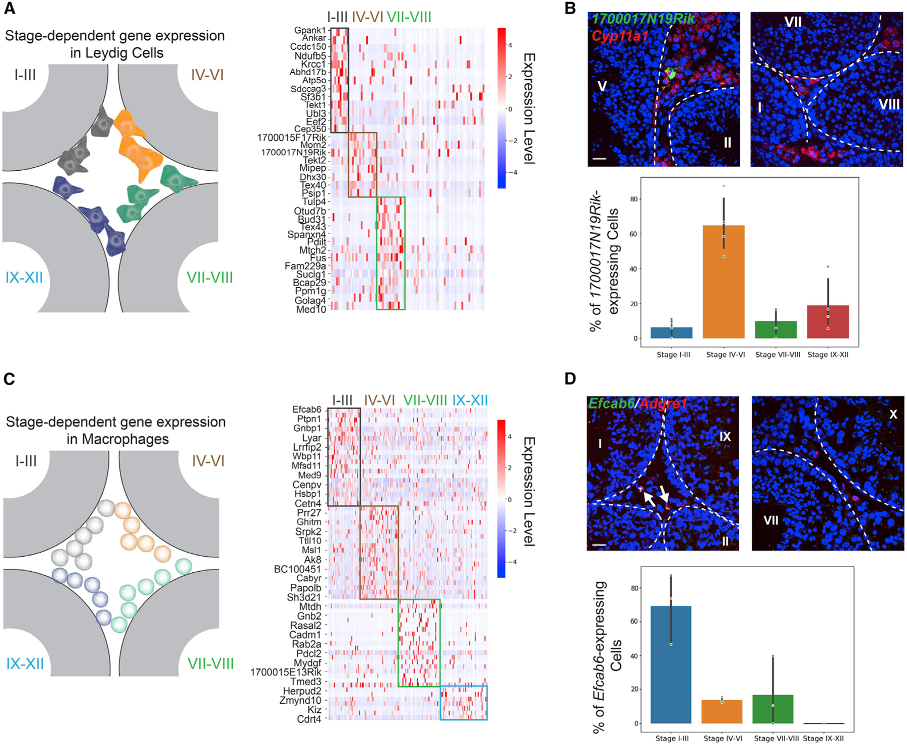
(A) Left: schematic of the spatial localizations of Leydig cells. Right: genes exhibiting stage-dependent expression patterns in Leydig cells.

(B) Upper panel:1700017N19Rik-expressing Leydig cells (marked by Cyp11a1) localize near a stage IV–VI seminiferous tubule, but not close to tubules at other stages. The basement membrane is outlined by white dashed lines. Scale bar, 20 μm. Lower panel: bar graph summarizing the percentages of 1700017N19Rik-expressing Leydig near seminiferous tubules at different stage groups. One-way ANOVA, p < 10⁻⁴, n = 4 biological replicates.

(C) Left: schematic of the spatial localizations of macrophages. Right: genes exhibiting stage-dependent expression patterns in macrophages.

(D) Upper panel: Efcab6-expressing macrophages (marked by Adgre1) localize near stage I–III seminiferous tubules, but not close to tubules at other stages. The basement membrane is outlined by white dashed lines. Scale bar, 20 μm. Lower panel: bar graph summarizing the percentages of Efcab6-expressing macrophages near seminiferous tubules at different stage groups. One-way ANOVA, p < 0.005. n = 3 biological replicates.

Similar to the analysis done on the Leydig cells, a differential gene expression analysis was performed on the macrophage populations (Figure 3C). We then used smFISH to confirm the stage-specific expression pattern of Efcab6 (Figure 3D; one-way ANOVA, p < 0.005). Moreover, recent studies have uncovered two populations of macrophages from two distinct lineages, with one population localized in the interstitial space and the other in the peritubular space (DeFalco et al., 2015; Mossadegh-Keller et al., 2017). We distinguished these two populations in the spatial transcriptome atlas based on their relative spatial position with Leydig cell beads, since Leydig cells are known to occupy the interstitial space (Figure S3B; STAR Methods). Indeed, we found that beads assigned as peritubular macrophages exclusively expressed H2-Ab1 and Il1b genes (Figure S3C), consistent with previous findings that these two genes are marker genes for peritubular macrophages (Mossadegh-Keller et al., 2017). Together, we demonstrated how the cycle of the seminiferous epithelium influenced the molecular compositions of Leydig cells and macrophages by identifying the stage-dependent gene expression programs. Our analysis also successfully distinguished the two lineages of testicular macrophages based on their spatial localization.

Building a spatial transcriptome atlas for human spermatogenesis

Given the successful establishment of the mouse testicular spatial transcriptome atlas, we next used the same computational pipeline to spatially map human testicular cell types (Figure S4A). The accuracy of the cell-type assignment was validated by the enrichment of cell-type marker genes (Figure S4C). Moreover, the structure of the reconstructed pseudotime image using the human Slide-seq data agreed with the morphology of the adjacent cross section (Figure S4B). Using the same method, we identified 788 human SP genes (Table S1; examples are shown in Figures S4D and S4E), of which 580 genes showed matching spatial expression patterns with data from the Human Protein Atlas (https://www.proteinatlas.org/) (Uhlén et al., 2015). The rest of genes were either not covered in the database or showed nonspecific immunostaining signals. We further validated some of these SP genes, including ACTRT3, ACRBP, CLDN11, LPIN1, and TNP1, using smFISH (Figure S4F). Finally, GO enrichment analysis of human SP genes showed that they were enriched in RNA processing and protein targeting pathways, as well as pathways regulating spermatid development and differentiation (Figure S4G).

Spatial profiling of the spermatogonial microenvironment with in situ RNA sequencing

The spermatogonia (SPG) contain the stem cell population. Previous studies have suggested that the self-renewal and differentiation of SPG is influenced by their surrounding microenvironment (Phillips et al., 2010; de Rooij, 2017). To systematically profile the spermatogonial microenvironment, we first spatially mapped populations of undifferentiated and differentiating SPG in both the mouse (Figures 4A and S5A) and human (Figures 4E and S5F) testis. Using a K-nearest neighbor (KNN)-based approach (Figure 4B; STAR Methods), we calculated the cellular compositions of the microenvironment surrounding each SPG. We found that in both mouse and human testis, undifferentiated and differentiating SPGs are in spatial proximity to themselves while also spatially segregating with each other (Figures 4B and 4F). Next, we asked if the spatial compositions of non-SPG cell types differ in the microenvironment surrounding the undifferentiated versus differentiating SPGs. Of interest, we observed no such difference in the mouse testis (Figure 4B). This observation was consistent across different Ks (K = 5, 10, and 15) and three replicates (Figures S5B and S5C). To perform a microscopy-based measurement of the spermatogonial microenvironment, we performed in situ RNA sequencing targeting 22 genes simultaneously in the mouse testis, with 12 cell-type-specific marker genes (Figures 4C and S5D). This independent dataset further supported the finding from the Slide-seq data (Figures 4D and S5E). The similar spatial composition of non-SPG cell types prompted us to examine if non-SPG cell types in the two SPG microenvironment are at different cellular states. To this end, we devised a differential gene expression test (STAR Methods), which, of interest, did not yield significantly differentially expressed (DE) genes (Table S3), suggesting that non-SPG cells surrounding undifferentiated and differentiating SPGs are at similar transcriptional states. Together, our data suggested a mouse spermatogonial microenvironment where spatially segregated spermatogonial subpopulations are exposed to seemingly uniformly distributed extracellular signals.

Figure 4. Differential stem cell microenvironment in mouse versus human testes.

(A) Spatial mapping of mouse undifferentiated and differentiating spermatogonia using the Slide-seq data. Scale bar, 300 μm.

(B) K nearest neighbor (KNN) approach to calculate cell-type compositions in the microenvironment surrounding each mouse spermatogonium using Slide-seq data. Comparison of cell-type compositions of the microenvironment surrounding undifferentiated versus differentiating spermatogonia with K = 5 neighbors is shown here. Plots showing K = 10 and 15 are shown in Figure S5B. Two additional biological replicates are shown in Figure S5C. n.s., not significant; ES, elongating/elongated spermatids; RS, round spermatids; SPC, spermatocytes; Diff SPG, differentiating spermatogonia; Undiff SPG, undifferentiated spermatogonia.

(C) In situ sequencing of mouse testis samples targeting 22 genes. ES, elongating/elongated spermatids; RS, round spermatids; Diff SPG, differentiating spermatogonia; Undiff SPG, undifferentiated spermatogonia; Endo, endothelial cells. White dashed lines outline the seminiferous tubules in the image. Scale bars represent 20 μm (2 μm for the inset).

(D) KNN calculation of cell-type compositions of microenvironment surrounding mouse undifferentiated versus differentiating spermatogonia using data generated in (C). K = 5 neighbors was used. Plots showing K = 10 and 15 are shown in Figure S5E. n.s., not significant; ES, elongating/elongated spermatids; RS, round spermatids; SPC, spermatocytes; Diff SPG, differentiating spermatogonia; Undiff SPG, undifferentiated spermatogonia.

(E) Spatial mapping of human undifferentiated and differentiating spermatogonia using the Slide-seq data. Scale bar, 300 μm.

(F) Comparison of cell-type compositions of the microenvironment surrounding human undifferentiated versus differentiating spermatogonia. K = 10 neighbors was used. Plots showing K = 15, as well as for a different replicate are shown in Figure S5G. n.s., not significant; ES, elongating/elongated spermatids; RS, round spermatids; SPC, spermatocytes; Diff SPG, differentiating spermatogonia; Undiff SPG, undifferentiated spermatogonia.

(G) Comparison in endothelial cell composition of microenvironment surrounding human undifferentiated versus differentiating spermatogonia using multiplexed smFISH data. Diff SPG, differentiating spermatogonia; Undiff SPG, undifferentiated spermatogonia. Red arrowhead, endothelial cells; magenta arrowhead, undifferentiated spermatogonium; green arrowhead, differentiating spermatogonium. White dashed lines outline the seminiferous tubules in the image. Scale bars represent 70 μm (10 μm for the inset).

To our surprise, in contrast to the mouse, we found significant differences in the spatial cellular compositions of the microenvironment surrounding the human undifferentiated versus differentiating SPGs (Figures 4F and S5G). This was especially true for somatic cell types such as Leydig cells, endothelial cells, and macrophages, but not for Sertoli cells and myoid cells, suggesting potentially differential roles in shaping the spermatogonial microenvironment among these somatic cell types in the human testis. Finally, we confirmed this finding using multiplexed smFISH, showing differential enrichment of endothelial cells in the microenvironment surrounding the human undifferentiated versus differentiating SPGs (Figure 4G). Together, our data revealed significant differences in the spatial structure of the spermatogonial microenvironment between mouse and human, indicating differential regulatory mechanisms governing the early stage of spermatogenesis between the two species.

Diabetes induces testicular injuries by disrupting the spatial structures of seminiferous tubules

Finally, we envisioned that the Slide-seq workflow and the accompanying computational pipelines could also be applied to profile pathological changes in spermatogenesis. To this end, we generated Slide-seq data from three leptin-deficient diabetic mice (ob/ob) and three matching wild-type (WT) mice (one representative dataset is shown in Figure 5A). An important complication of diabetes mellitus (DM) is the disturbance in the male reproductive system. Numerous reports are available on impaired spermatogenesis under diabetic conditions (Alves et al., 2013; Ding et al., 2015; Jangir and Jain, 2014; Maresch et al., 2019), although the underlying mechanisms have not been fully appreciated. We first used the Slide-seq data to identify DE genes between the ob/ob and WT samples in each testicular cell type (Table S3). We found that genes mainly expressed in ESs such as Prm1, Prm2, Odf1, and Smcp were significantly downregulated in the ob/ob testes, consistent with the phenotype of ES/spermatozoon loss in ob/ob testes reported by a previous study (Bhat et al., 2006). In contrast, multiple mitochondrial genes such as mt-Nd1, mt-Rnr1, and mt-Rnr2, as well as the non-coding RNA Malat1, were among the genes whose expression was significantly elevated in ob/ob testes. This was also consistent with the observations that the increased expression levels of mitochondrial-encoded genes were associated with mtDNA damage and mitochondrial dysfunction in the pathogenicity of DM (Antonetti et al., 1995) and that the expression of Malat1 was elevated in multiple diabetic-related diseases (Abdulle et al., 2019). In addition, we also found genes involved in meiosis such as Ubb, Mael, and Hspa2 were DE, which echoed the findings in the ovary, where meiotic regulation in oocytes was altered in diabetic mice and rats (Colton et al., 2002; Kim et al., 2007). Together, these results demonstrated the ability of the spatial transcriptome atlas to capture the molecular changes in diabetic testes.

Figure 5. Diabetes causes disruptions in spatial arrangements of testicular cell types in the seminiferous tubules.

(A) Spatial mapping of testicular cell types for wild-type (WT) and ob/ob samples. Scale bar, 500 μm.

(B) The spatial expression pattern of Smcp is disrupted in a representative ob/ob seminiferous tubule. ES, elongating/elongated spermatid; RS, round spermatid; SPC, spermatocyte; SPG, spermatogonium. Scale bar, 30 μm.

(C) The ES purity score for each Slide-seq bead in a representative WT and ob/ob seminiferous tubule, respectively. The mean purity score for the beads with non-zero value in each tubule is also shown. Scale bar, 30 μm.

(D) The mean purity score for each seminiferous tubule with at least 50 ES beads from the WT and ob/ob samples (n = 3 biological replicates per condition). Comparison of the purity score between the two conditions was performed using the Mann-Whitney U test.

(E) Left: two clusters of WT seminiferous tubule structures revealed by the principal components of pairwise spatial contact frequencies in WT seminiferous tubules. The stage information of each tubule is labeled. Right: projection of ob/ob seminiferous tubules onto the two clusters shown in the left plot.

(F) Mann-Whitney U test (n = 3 biological replicates per condition) on pairwise spatial cellular contact frequencies between WT and ob/ob seminiferous tubules under the two clusters. Signed p values of significant increases (positive) and decreases (negative) in spatial contact frequencies between cell types are shown.

Next, we sought to spatially map the expressions of the identified DE genes. Of interest, we noticed that some of the DE genes, such as Smcp, Odf1, and Malat1, showed altered spatial expression patterns in ob/ob testis cross sections (Figures S5H and S5I). By zooming into individual seminiferous tubules, we found that the spatial expression pattern of Smcp was disrupted in ob/ob seminiferous tubules (Figure 5B). Since we have shown that the spatial expression pattern of Smcp was not stage dependent (Table S1), this disruption was not likely due to differences in stages of the seminiferous epithelium cycle. A close examination of the ob/ob tubules indicated that the changes in gene expression pattern were due in part (if not entirely) to an alteration in the spatial cellular organization, especially among the spermatid population. To profile such changes systematically and quantitatively in the ob/ob seminiferous tubules, we first devised a metric termed purity score to evaluate the extent of the spatial mixing between ES beads and beads of other cell types (STAR Methods). In a WT seminiferous tube, ES beads clustered together at the center, showing a high average purity score (Figure 5C, left). In contrast, such spatial organization was disrupted in the ob/ob seminiferous tubules, where ES beads were more likely to make spatial contacts with beads of other cell types, showing a low purity score (Figure 5C, right). We then calculated the average purity scores for 72 WT tubules and 136 ob/ob tubules across three replicates and found that the scores were significantly lower in ob/ob tubules than in WT tubules (Figure 5D; Mann-Whitney U test). Next, we quantified the spatial arrangements of all the cell types within a seminiferous tubule by calculating their pairwise spatial contact frequencies (STAR Methods). Principal-component (PC) analysis of the WT seminiferous tubules based on the pairwise spatial contact frequencies revealed two major clusters (Figure 5E, left, showing the first two PCs of the clusters). The separation of these two clusters was mainly contributed by differences in cell-type proportions under different stages of the seminiferous epithelium cycle (Figure 5E, left). We then clustered the ob/ob seminiferous tubules in the same PC space with the WT tubules (Figure 5E, right). By comparing each pairwise spatial contact frequency between the WT and ob/ob seminiferous tubules under the same cluster, we effectively eliminated the influence of the tubule stages on cell-type proportions. Consistent with the purity score measurement, we observed significant changes in the spatial arrangements between ES beads and beads of all other cell types (Figure 5F). Moreover, the spatial contacts between RSs and other cell types, especially macrophages, were also markedly enhanced in the ob/ob tubules (Figure 5F), suggesting that the spatial arrangement of spermatids was the most susceptible to the disruptive effects under diabetic conditions. Taken together, our analysis shows that the disruption of the spatial structure of seminiferous tubules is a potential mechanism of diabetes-induced testicular injuries.

DISCUSSION

Spermatogenesis takes place in the spatially confined environment of seminiferous tubules and is constantly influenced by the somatic cell types in the peritubular and interstitial space. However, there has been a lack of tools to comprehensively profile spermatogenesis within the native context of seminiferous tubules. Moreover, within any given testis cross section, each seminiferous tubule is at a specific stage, and each stage is associated with unique combinations of germ cell subtypes and biological events, making it challenging to obtain stage-specific spermatogenesis with molecular resolution. Using Slide-seq, we have generated an unbiased spatial transcriptome atlas for the mouse and human spermatogenesis at near-single-cell resolution. By applying a custom computational pipeline, we were able to assign information of cell type, seminiferous tubule, and stage to each Slide-seq bead with high accuracy. Our data provide a framework to systematically evaluate the spatial dynamics in gene expressions and in cellular structures both within and surrounding the seminiferous tubules with high resolution.

The spatial transcriptome atlas as a platform for profiling spatial gene expression dynamics in spermatogenesis

The testis expresses the largest number of genes of any mammalian organ, and many of these genes are testis specific (Brawand et al., 2011; Djureinovic et al., 2014; Melé et al., 2015). However, the localization and biological functions of these genes remain largely unexplored. Here, we show that the spatial transcriptome atlas is a powerful platform for profiling spatial gene expression dynamics. (1) Using the spatial atlas, we systemically localized genes at the level of individual seminiferous tubules in both the mouse and human testis. (2) We observed changes in the spatial expression pattern of the same gene under different stages of the seminiferous epithelium cycle. (3) Due to the cyclic nature of spermatogenesis and the availability of the stage information, we were able to use the spatial transcriptomic data to infer temporal expression dynamics of genes along the developmental trajectory of germ cells. This provided information on the germ cell developmental stages during which these genes are likely to exert their functions. (4) By grouping the SP genes based on their involvement in different signaling pathways, we nominated genes with previously underappreciated functions. (5) Besides SP genes, we used the spatial transcriptome atlas to also identify genes with stage-specific expression in two somatic cell types of the testis, Leydig cells and macrophages. These genes may exert their functions in a stage-dependent manner.

The spatial transcriptome atlas as a platform for profiling spatial cellular structures of seminiferous tubules

In both mouse and human testis, testicular cell types are spatially organized in a stereotypic pattern within and surrounding the seminiferous tubules to support spermatogenesis. In this study, we spatially mapped undifferentiated and differentiating SPG in mouse and human seminiferous tubules, respectively. A microenvironment analysis identified major differences in the patterns of cellular composition surrounding the undifferentiated and differentiating SPG between mouse and human testis. Future research on how these differences are linked to differential regulation of spermatogonial stem cell activities in the two species may provide insights into the regulatory mechanisms of mammalian spermatogenesis.

In addition to profiling normal testis samples, we also systematically compared the spatial cellular structures between WT and diabetic seminiferous tubules. By calculating the extent of spatial mixing and pairwise cell-cell contact frequencies between different cell types, we observed a significant disruption in the spatial cellular organization of the diabetic seminiferous tubules. Of interest, a previous study using second-order stereology has indicated that the spatial arrangement of Sertoli cells and SPG is significantly disrupted in the diabetic testes (Sajadi et al., 2019). Indeed, our analysis showed a significant change in the spatial contact frequencies between Sertoli cells and SPG. Taken together, a disruption in the spatial cellular organization at the level of seminiferous tubules may serve as a mechanism by which diabetes impairs male fertility. Although we only applied Slide-seq to the diabetic models, we envision that it can be readily adapted to profile the spatial cellular structures in other perturbation models as well as testicular biopsy specimens from infertile patients or patients with testicular cancers.

Limitations of study

Enhanced capture efficiency of testicular RNA would allow for higher statistical power for accurate cell-type assignment, such as assigning beads to myoid cells (which have narrow spindle-like shapes that may pose challenges for RNA capture); stage-dependent gene expression analysis in all testicular cell types, especially Sertoli cells; distinguishing subpopulations of SPG (e.g., Ngn3-negative and Ngn3-positive populations); and dissecting how these molecularly distinct subpopulations spatially interact with each other. Recent advances in machine learning approaches may enable even more accurate cell-type decomposition on each Slide-seq bead (Cable et al., 2021) and facilitate further investigation of cell-cell interactions, such as the spatial ligand-receptor relationship (Li et al., 2021).

In summary, the mouse and human testicular spatial transcriptome atlas is a valuable resource to comprehensively reveal the detailed spatial molecular and cellular information that instructs spermatogenesis. The Slide-seq protocol and analytical framework can be readily adapted to other stereotypically structured tissues and developing animals and might be applicable to more perturbation models as well.

STAR★METHODS

RESOURCE AVAILABILITY

Lead contact

Further information and requests for resources and reagents should be directed to and will be fulfilled by the lead contact, Fei Chen (chenf@broadinstitute.org).

Materials availability

Reagents generated in this study will be made available on request, considering the terms of materials transfer agreement (MTA) for the modified reagents. We may require a completed MTA if there is potential for commercial application.

Data and code availability

The raw sequencing data supporting the findings of this study are available in NCBI BioProject database with BioProject ID: PRJNA668433. The processed data including the gene expression matrices, bead location matrices, and the NMFreg-enabled cell type assignment matrices are available at https://www.dropbox.com/s/ygzpj0d0oh67br0/Testis_Slideseq_Data.zip?dl=0.

Custom code is available at https://github.com/thechenlab/Testis_Slide-seq.

Any additional information required to reanalyze the data reported in this paper is available from the lead contact upon request.

EXPERIMENTAL MODEL AND SUBJECT DETAILS

Mice

All animal experiments were carried out with prior approval of the Broad Institute of MIT and Harvard on Use and Care of Animals (Protocol ID: 0211-06-18), in accordance with the guidelines established by the National Research Council Guide for the Care and Use of Laboratory Animals. The following mice were purchased from the Jackson laboratories: C57BL/6J (JAX, #000664) and B6.Cg-Lepob/J (JAX #000632). Mice were housed in the Broad Institute animal facility, in an environment controlled for light (12 hours on/off) and temperature (21 to 23°C) with ad libitum access to water and food. Testicular tissues were harvested from adult male mice of 3–10-month-old.

Human testicular biopsies

Adult human testicular samples for Slide-seq and smFISH were from two healthy men (donor #1: 25 years old; donor #2: 32 years old); Samples were obtained through the University of Utah Andrology laboratory and Intermountain Donor Service. Both samples were de-identified.

METHOD DETAILS

Transcardial Perfusion

Mice were anesthetized by administration of isoflurane in a gas chamber flowing 3% isoflurane for 1 minute. Anesthesia was confirmed by checking for a negative tail pinch response. Animals were moved to a dissection tray and anesthesia was prolonged via a nose cone flowing 3% isoflurane for the duration of the procedure. Transcardial perfusions were performed with ice cold pH 7.4 PBS to remove blood from the testes. Testes were removed and frozen for 3 minutes in liquid nitrogen vapor and moved to −80°C for long term storage.

Slide-seq workflow

The workflow of Slide-seq was described previously (Stickels et al., 2021). Briefly, the 10-μm polyT barcoded beads were synthesized in house. Each bead oligo contains a linker sequence, a spatial barcode, a UMI sequence, and a polyT tail. The bead arrays were prepared by pipetting the synthesized beads which were pelleted and resuspended in water + 10% DMSO at a concentration between 20,000 and 50,000 beads/μL, into each position on a gasket. The coverslip-gasket filled with beads was then centrifuged at 40°C, 850 g for at least 30 minutes until the surface was dry. In situ sequencing of the bead array to extract the spatial barcodes on the beads were performed in a Bioptechs FCS2 flow cell using a RP-1 peristaltic pump (Rainin), and a modular valve positioner (Hamilton MVP). Flow rates between 1 mL/min and 3 mL/min were used during sequencing. Imaging was performed using a Nikon Eclipse Ti microscope with a Yokogawa CSU-W1 confocal scanner unit and an Andor Zyla 4.2 Plus camera. Images were acquired using a Nikon Plan Apo 10x/0.45 objective. Sequencing was performed using a sequencing-by-ligation approach. Image processing was performed using a custom MATLAB package (https://github.com/MacoskoLab/PuckCaller/).

Fresh frozen testis tissue was warmed to −20°C in a cryostat (Leica CM3050S) for 20 minutes prior to handling. Tissue was then mounted onto a cutting block with OCT and sliced at 10 μm thickness. Sequenced bead arrays were then placed on the cutting stage and tissue was maneuvered onto the pucks. The tissue was then melted onto the array by moving the array off the stage and placing a finger on the bottom side of the glass. The array was then removed from the cryostat and placed into a 1.5 mL eppendorf tube. The sample library was then prepared as below. The remaining tissue was re-deposited at −80°C and stored for processing later.

Bead arrays with tissue sections were immediately immersed in 200 μL of hybridization buffer (6x SSC with 2 U/μL Lucigen NxGen RNase inhibitor) for 30 minutes at room temperature to allow for binding of the mRNA to the oligos on the beads. Subsequently, first strand synthesis was performed by incubating the pucks in 200 μL of reverse transcription solution (Maxima 1x RT Buffer, 1 mM dNTPs, 2 U/μL Lucigen NxGen RNase inhibitor, 2.5 μM template switch oligo with QIAGEN #339414YCO0076714, 10 U/μL Maxima H minus reverse transcriptase) for 1.5 hours at 52°C. 200 μL of 2x tissue digestion buffer (200 mM Tris-Cl pH 8, 400 mM NaCl, 4% SDS, 10 mM EDTA, 32 U/mL Proteinase K) was then added directly to the reverse transcription solution and the mixture was incubated at 37°C for 30 minutes. The solution was then pipetted up and down vigorously to remove beads from the glass surface, and the glass substrate was removed from the tube using forceps and discarded. 200 μL of wash buffer (10 mM Tris pH 8.0, 1 mM EDTA, 0.01% Tween-20) was then added to the solution mix and the tube was then centrifuged for 3 minutes at 3000 RCF. The supernatant was then removed from the bead pellet, the beads were resuspended in 200 μL of wash buffer and were centrifuged again. This was repeated a total of three times. The supernatant was then removed from the pellet. The beads were then resuspended in 200 μL of 1 U/μL Exonuclease I and incubated at 37°C for 50 minutes. After Exonuclease I treatment the beads were centrifuged for 3 minutes at 3000 RCF. The supernatant was then removed from the bead pellet, the beads were resuspended in 200 μL of wash buffer and were centrifuged again. This was repeated a total of three times. The supernatant was then removed from the pellet. The pellet was then resuspended in 200 μL of 0.1 N NaOH and incubated for 5 minutes at room temp. To quench the reaction 200 μL of wash buffer was added and beads were centrifuged for 3 minutes at 3000 RCF. The supernatant was then removed from the bead pellet, the beads were resuspended in 200 μL of wash buffer and were centrifuged again. This was repeated a total of three times. Second strand synthesis was then performed on the beads by incubating the pellet in 200 μL of second strand mix (Maxima 1x RT Buffer, 1 mM dNTPs, 10 μm dN-SMRT oligo, 0.125 U/μL Klenow fragment) at 37°C for 1 hour. After the second strand synthesis 200 μL of wash buffer was added and the beads were centrifuged for 3 minutes at 3000 RCF. The supernatant was then removed from the bead pellet, and the beads were resuspended in 200 μL of wash buffer and were centrifuged again. This was repeated a total of three times. 200 μL of water was then added to the bead pellet and the beads were moved into a 200 μL PCR strip tube, pelleted in a minifuge, and resuspended in 200 μL of water. The beads were then pelleted and resuspended in PCR mix (1x Terra Direct PCR mix buffer, 0.25 U/μL Terra polymerase, 2 μM Truseq PCR handle primer, 2 μM SMART PCR primer) and PCR was performed using the following program: 95°C 3 minutes; 4 cycles of: 98°C for 20 s, 65°C for 45 s, 72°C for 3 min and 9 cycles of: 98°C for 20 s, 67°C for 20 s, 72°C for 3 min; 72°C for 5 min and hold at 4°C. The PCR product was then purified using 30 μL of Ampure XP beads (Beckman) according to manufacturer’s instructions and resuspended into 50 μL of water and the cleanup was repeated and resuspended in a final volume of 10 μL. 1 μL of the library was quantified on an Agilent Bioanalyzer High sensitivity DNA chip (Agilent). Then, 600 pg of PCR product was prepared into Illumina sequencing libraries through tagmentation with a Nextera XT kit (Illumina). Tagmentation was performed according to manufacturer’s instructions and the library was amplified with primers Truseq5 and N700 series barcoded index primers. The PCR program was as follows: 72°C for 3 min and 95°C for 30 s; 12 cycles of: 95°C for 10 s, 55°C for 30 s, 72°C for 30 s; 72°C for 5 min and hold at 10°C. Samples were cleaned with Ampure XP beads in accordance with manufacturer’s instructions at a 0.6x bead/sample ratio (30 μL of beads to 50 μL of sample) and resuspended in 10 μL of water. Library quantification was performed using the Bioanalyzer. Finally, the library concentration was normalized to 4 nM for sequencing. Samples were sequenced on the Illumina NovaSeq S2 flow cell 100 cycle kit with 12 samples per run (6 samples per lane) with the read structure 42 bases Read 1, 8 bases i7 index read, 50 bases Read 2. Each bead array received approximately 150–200 million reads, corresponding to ~2,000–2,500 reads per bead.

Targeted in situ RNA sequencing

The in situ RNA sequencing protocol was adapted from previous studies (Alon et al., 2021; Payne et al., 2021). The inner surface of a glass-bottom plate was incubated for 1 minute with 3-(Trimethoxysilyl) propyl methacrylate (Sigma) diluted 1:1000 in 80% ethanol, 2% acetic acid, 18% H2O, and then washed 3 times in ethanol to functionalize the glass surface with methacrylate moieties. Frozen mouse testis sections at 10 μm thickness were placed in the coated wells and were fixed in 10% Formalin for 15 min at room temperature. Following two washes with PBS at room temperature, permeabilization of tissues was done with ice-cold 70% EtOH for 2 hr - overnight at −20°C. After 3 washes with PBS, sections were preconditioned for 30 min at room temperature with the wash buffer (2X SSC, 20% formamide (v/v)) supplemented with 0.4 U/μl RNase Inhibitor (Lucigen). Pooled padlock probes targeting 22 genes (probe sequences available in Table S4) were diluted in the wash buffer so that each padlock probe was at 0.1 μM final concentration. 200 μL of probe solution was applied to each well and the sections were incubated overnight at 37°C. After 3 washes with the wash buffer at 37°C (30 min each) and 1 wash with PBS for 30 min at 37°C, sections were equilibrated with 1X SplintR ligase buffer (NEB) at room temperature for 30 min. Sections were then incubated with SplintR ligase (NEB) at a concentration of 1.25U/μL at 37°C for 6 hr - overnight. Following a wash in 2X SSC buffer for 30 min at room temperature, a 500 nM rolling circle amplification (RCA) primer solution (TCTTCAGCGTTCCCGA*G*A, *phosphorothioates; prepared in the wash buffer) was incubated with sections for 2 hr at 37°C. After a wash with the wash buffer for 30 min at 37°C, a wash with 1XPBS for 15min at 37°C, and a wash with 1X Phi29 Buffer (QIAGEN) for 15 min at room temperature, an RCA mix (1X Phi29 Buffer, 250 μM dNTP (NEB), 40 μM Aminoallyl dUTP (aa-dUTP, ThermoFisher) and 1 U/μL Phi29 DNA Polymerase (QIAGEN)) was applied to sections and incubated for overnight at 30°C. The reaction was terminated by washing the sections with 1X PBS for 30 min, and a crosslinking mix (5 mM BS(PEG)9 (ThermoFisher) in PBS) was incubated with the sections for 2 hr at room temperature. The reaction was then quenched by washing with 1 M Tris pH 8 for 15 min at room temperature. To detect RCA products, sections were washed with the wash-10 buffer (2X SSC, 10% formamide (v/v) in water) for 20 min at room temperature, and incubated with a 100 nM amplicon detection probe solution (/5Alex546N/TCTCGGGAACGCTGAAGA, prepared in the wash-10 buffer) for 1 hr at 37°C. Following a wash with the wash-10 buffer for 20 min at 37°C and a wash in 1X PBS for 20min at 37°C, sections were imaged using a 40X water objective. After imaging, a stripping solution (80% formamide (v/v), 0.01% Triton X-100 (v/v) in water) heated to 80°C was used to wash the sections 3 times with for 10 min each at room temperature. The sections were then washed twice with 1X PBS for 10 min each.

To perform tissue clearing, a cut piece of a glass microscope slide, which would be used in casting the polyacrylamide gels, was incubated with Sigmacote (Sigma) for 1 minute and then washed 3 times in H₂O to make the surface hydrophobic. Near each edge of the hydrophobic glass, two layers of Invisible Tape (Universal) were attached to the glass to form spacers roughly 100 μm thick. A preincubation solution (4% acrylamide/bis 19:1, 40% (w/v) (VWR), 1X PBS, 0.2% (w/v) ammonium persulfate (Sigma), 0.2% (w/v) N,N,N′,N′-tetramethylethylenediamine (Sigma), 0.005% (w/v) 4-Hydroxy-TEMPO (Sigma)) was first applied to the sections and was incubated at 4°C for 30 min. Next, 10 μL of gelation solution (4% acrylamide/bis 19:1, 40% (w/v) (VWR), 1X PBS, 0.2% (w/v) ammonium persulfate (Sigma), 0.2% (w/v) N,N,N′,N′-tetramethylethylenediamine (Sigma)) was added to cover each section and the taped hydrophobic glass was immediately applied over the gelation solution to form a gelation chamber. The samples were put on a hot plate at 45°C for 3 min and were then transferred into a humidified container and incubated for 2 hr at 37°C. Finally, the glass was removed, and the sections were digested with a digestion solution (50 mM Tris pH 8.0, 1mM EDTA, 0.5% (v/v) Triton X-100, 500mM NaCl, 8U/mL Proteinase K) overnight at room temperature.

To perform in situ sequencing, the sections were first washed four times with the instrument buffer (50 mM Tris acetate, pH 7, 0.05% (v/v) Triton X-100) at room temperature. The sections were then treated with QuickCIP solution (1X CutSmart buffer, 250U/mL QuickCIP (NEB)) for 45 min at room temperature, followed by five washes with the instrument buffer for 5 min each. A 2.5 μM sequencing primer solution (/5phos/TCTCGGGAACGCTGAAGA for round 1 and 2; /5phos/CTCGGGAACGCTGAAGA for round 3 and 4; /5phos/TCGGGAACGCTGAAGA for round 5) was prepared by diluting the 100 μM primer stock into the 5X SASC buffer (0.75 M sodium acetate, 75 mM sodium citrate, pH7.5). The sections were incubated with the sequencing primer solution for 45 min at room temperature, followed by 2 washes with the instrument buffer at room temperature. The sections were then incubated with a ligation mix of 1X T4 DNA ligase buffer (QIAGEN), 1 mg/mL UltraPure BSA (ThermoFisher), 60 U/μL Rapid T4 DNA ligase (QIAGEN), 1:200 dilution of SOLiD sequencing oligos (ThermoFisher) for 90 min at room temperature, followed by 3 washes with the instrument buffer at room temperature.

Sequencing was performed using an inverted Nikon CSU-W1 Yokogawa spinning disk confocal microscope using a Nikon CFI APO LWD 40X/1.15 water immersion objective and an Andor Zyla sCMOS camera. Images were acquired in the following channels: 488-nm excitation with a 525/36-nm emission filter (MVI, 77074803), 561-nm excitation with a 582/15-nm emission filter (MVI, FF01-582/15-25), 561-nm excitation with a 624/40-nm emission filter (MVI, FF01-624/40-25) and 647-nm excitation with a 705/720-nm emission filter (MVI, 77074329). NIS-Elements AR software (v4.30.01, Nikon) was used for image capture. A total of 12 fields of views (FOVs) were captured with an interval of 0.4 μm at the z axis. The sections were incubated with the QuickCIP solution for 45 min at room temperature after each round of sequencing. Following the 1st and the 3rd round of sequencing, a cleavage step was performed to expose the 5′ phosphates for the next round of ligation. The cleavage was done by first treating the sections with the cleavage-1 buffer (50 mM AgNO₃ in water) twice for 5 min each at room temperature and then by incubating the sections twice with the cleavage-2 buffer (50 mM 2-mercaptoethanolsulfate, 30 mM sodium citrate, 300 mM sodium acetate, pH 7.5) for 5 min each at room temperature. After the 2nd and the 4th round of sequencing, the sequencing primers were stripped by incubating the sections with the stripping solution twice for 10 min each as described before. DAPI stain was performed before each round of sequencing.

Immunofluorescence

Slides with tissue sections were fixed in 4% PFA (in PBS) and washed three times in PBS for 5 minutes each, blocked 30 minutes in 4% BSA (in PBST), incubated with primary antibodies overnight at 4°C, washed three times in PBS for 5 minutes each, and then incubated with secondary antibodies at for 1 hour at room temperature. Slides were then washed twice in PBS for 5 minutes each and then for 10 minutes with a PBS containing DAPI (D9542, Sigma-Aldrich). Lastly, slides were mounted using ProLong Gold Antifade Mountant (P36934, Thermo Fisher Scientific) and sealed. Antibodies used for IF: Rabbit Anti-HABP4 antibody (1:100, HPA055969, Millipore Sigma), mouse anti-phospho-histone H2A.X (Ser139) antibody, FITC conjugate (1:100, 16-202A, Millipore Sigma), Sheep anti-acetyl histone H4 antibody (1:100, AF5215, R&D Systems), and Alexa Fluor 594-, and 647-conjugated secondary antibodies (Thermo Fisher Scientific) were used.

Single Molecule RNA HCR

Single molecule RNA HCR was performed as described by Choi et al. (2018) with small modifications. Briefly, frozen testes were sectioned into (3-Aminopropyl) triethoxysilane-treated glass bottom 24-well plates. Sections were cross-linked with 10% Formalin for 15 min, washed with 1X PBS for three times, and permeabilized in 70% ethanol for 2 hours - overnight at −20°C. Sections were then rehydrated with 2X SSC (ThermoFisher Scientific) for three times and equilibrated in HCR hybridization buffer (Molecular Instruments, Inc.) for 10 minutes at 37°C. Gene probes were added to the sections at a final concentration of 2 nM in HCR hybridization buffer and hybridized overnight in a humidified chamber at 37°C. Custom probe sets were designed and synthesized by Molecular Instruments, Inc. After hybridization, samples were washed four times in HCR wash buffer (Molecular Instruments, Inc.) for 15min at 37°C and then three times for 5 minutes at room temperature in 5X SSCT (ThermoFisher Scientific). The probe sets were amplified with HCR hairpins for 12–16 hours at room temperature in HCR amplification buffer (Molecular Instruments, Inc.). Fluorescently-conjugated DNA hairpins used in the amplification were ordered from Molecular Instruments, Inc.. Prior to use, the hairpins were ‘snap cooled’ by heating at 95°C for 90 s and letting cool to room temperature for 30 min in the dark. After amplification, the samples were washed in 5X SSCT and stained with 20ng/mL DAPI (Sigma) before imaging. Microscopy was performed using an inverted Nikon CSU-W1 Yokogawa spinning disk confocal microscope with 488 nm, 640nm, 561nm, and 405 nm lasers, a Nikon CFI APO LWD 40X/1.15 water immersion objective, and an Andor Zyla sCMOS camera. NIS-Elements AR software (v4.30.01, Nikon) was used for image capture.

Computational Methods for Slide-seq Data

Preprocessing of Slide-seq Data

The Slide-seq tools (https://github.com/MacoskoLab/slideseq-tools) were used for processing raw sequencing data. In brief, the Slide-seq tools extracted the barcode for each read in an Illumina lane from Illumina BCL files, collected, demultiplexed, and sorted reads across all of the tiles of a lane via barcode, and produced an unmapped bam file for each lane. The bam file was tagged with cellular barcode (bead barcode) and molecular barcode (UMI). Low-quality reads were filtered, and reads were trimmed with starting sequence and adaptor-aware poly A. STAR (Dobin et al., 2013) was used to align reads to genome sequence. The unmapped bam and sorted aligned bam were merged and tagged with interval and gene function. For each of those barcodes with short read sequencing, hamming distances were calculated between it and all the bead barcodes from in situ sequencing. The list of unique matched Illumina barcodes with hamming distance ≤ 1 along with the matched bead barcodes were outputted. The final output from the Slide-seq tools were a digital gene expression matrix (bead barcodes X genes) and barcode location matrix (bead barcodes X spatial coordinates). For each Slide-seq bead, the total number of UMIs were calculated and beads with less than 20 UMIs were filtered out. A trimming step was also applied to exclude beads located outside the main bead array area.

Gene Count Normalization

To normalize the Slide-seq gene count data, we calculated the Pearson residuals (response residuals divided by the expected standard deviation) by fitting the UMI count data into a regularized negative binomial regression model where cellular sequencing depth is utilized as a covariate in a generalized linear model (Hafemeister and Satija, 2019). These Pearson residuals can be treated as normalized gene expression levels. Positive residuals for a given gene in each cell indicate that more UMIs than expected are observed given the gene’s average expression in the population and cellular sequencing depth, while negative residuals indicate the converse. This approach omits the need for heuristic steps including pseudocount addition or log-transformation and ensures that both lowly and highly expressed genes are transformed onto a common scale. We used the R package sctransform implemented in Seurat v3 to calculate the Pearson residuals which are referred to as expression level throughout all the graphs in the figures unless otherwise indicated.

Cell Type Assignment

To accurately assign cell type to each Slide-seq bead, the contribution of each cell type to the RNA on the bead was computed using a custom method, termed NMFreg (Non-Negative Matrix Factorization Regression) (Rodriques et al., 2019). The method consisted of two main steps: first, single-cell atlas data previously annotated with cell type identities was used to derive a basis in reduced gene space (via NMF), and second, non-negative least-squares (NNLS) regression was used to compute the loadings for each bead in that basis. To perform NMF on the mouse slide-seq data, we used scRNA-seq data from a study by Green et al. (2018). For the human, we used data from Guo et al. as a reference (Guo et al., 2018). The cell type of the bead was assigned based on the identity of the maximum factor loading determined by NMFreg.

Pseudotime Reconstruction

To assign pseudotime value to each Slide-seq bead, first we took a testicular germ cell scRNA-seq dataset as an input and assigned a pseudotime value to each cell from that dataset using Monocle (Qiu et al., 2017). For the mouse, we used a published scRNA-seq dataset from Lukassen et al. (2018). For the human, we used the data from Guo et al. (2018). Next, we used Monocle to identify 1000 genes whose expression changed as a function of pseudotime. We then selected genes whose expression co-varied the most with pseudotime using L1 regularization. For the mouse data, we iterated the feature selection process through 1–20 genes and selected 14 genes which minimized the number of genes to be used while maximizing the fidelity of pseudotime reconstruction. The resulting linear function returned by L1 regularization included 6 genes with negative weights (hereafter referred as negative genes) and 8 genes with positive weights (positive genes) (Figure S1C). The negative genes and the corresponding coefficients are: mt-Nd1: 2.240772116330779, Tuba3b: 20.0, Stmn1: 4.661355144844998, Cypt4: 2.914946084728282, mt-Cytb: 7.940721195057547, Hsp90aa1: 7.719926741335844; The positive genes and the corresponding coefficients are Tnp2: 2.2300113564016115, Smcp: 20.0, Gsg1: 10.749147113890643, Oaz3: 13.684470608169942, Hmgb4: 11.19717467780924, Lyar: 3.205774497366639, Prm1: 1.8021648809899742, Dbil5: 2.4081140269931445. For the human, we selected 11 negative genes and 6 genes with positive genes. The negative genes and the corresponding coefficients are TNP1: 0.9106007166752985, RPL39: 9.212049749934977, PTGDS: 5.771773680502793, RPLP2: 20.0, FTH1: 19.992459791415897, MALAT1: 17.76205459561361, DCN: 19.475013103219712, RPLP1: 18.860848405765406, CFD: 7.067158789040227, FTL: 16.55433814467757; The positive genes and their corresponding coefficients are TSACC: 1.3896196907421736, NUPR2: 20.0, TMSB4X: 3.638712833769793, PRM2: 1.2032600855690998, PRM1: 0.4449200139269451. We then extracted the UMI count for each gene in the gene list from the Slide-seq data and multiplied that with the corresponding weight. The pseudotime value for each slide-seq bead was calculated by summing the weighted UMI count value from every gene in the gene list. Figure 1E was constructed using the Slide-seq beads assigned as germ cells. We also calculated the pseudotime values for the somatic cell types using the same genes and weights as described above. However, these values for somatic cells do not indicate that they are in the same developmental trajectory as the germ cells. Rather, they are solely used for the purpose of seminiferous tubule segmentation as described below.

Segmentation of Seminiferous Tubules

The fact that the image of pseudotime reconstruction retains the morphological structure of seminiferous tubules suggests that the image can be used to extract tubule information. Each slide-seq bead can be treated as a pixel and the pseudotime value assigned to each bead can be viewed as the pixel value. To this end, we developed a custom computational pipeline to first convert the bead pseudotime data into a grayscale image. Next, the grayscale image was smoothed using Gaussian blur with a sigma of 2. The smoothed image was then thresholded with an arbitrary pixel value cutoff which isolated individual tubes while retaining a maximum number of pixels passing the threshold. This was followed by a standard watershed workflow to find local maxima, perform distance transform, and segment individual seminiferous tubules. Finally, we performed K-nearest neighbor analysis to assign beads which were excluded during the thresholding step back to the nearest tubules. The segmented tubules were plotted and visually inspected. Wrongly assigned beads (for example, ES beads belonging to an adjacent seminiferous tubule but assigned to the periphery of the tubule inspected; beads assigned as Leydig cells, myoid cells, endothelial cells and macrophages but found within the seminiferous tubules) were excluded for subsequent analysis. This filtering was done to data from both the WT and ob/ob samples under the assumption that under both conditions the germline cells should localize within the confinement of seminiferous tubules and cells at the interstitial space should not be able to enter the tubules. We also excluded beads with low cell type certainty as determined in the NMFreg step (that is, the maximum loading of the cell type < 0.2). The number of beads excluded in this step for each sample is shown in Table S2.

Assignment of stages

Segmented seminiferous tubules with a total number of beads less than 20 and more than 700 were first filtered out. This was because tubules with less than 20 beads usually only represented a small portion of a tubule and tubules containing more than 700 beads represented two tubules which were not properly separated by the algorithm. Next, the raw UMI count data was normalized and variance-stabilized using the function SCTransform for Seurat V3 (Hafemeister and Satija, 2019). The normalized gene expression values of the Slide-seq beads within the same tubule were aggregated. Uniform manifold approximation and projection (UMAP) for dimension reduction of the aggregated gene expression data were performed using the top 3000 highly variable genes (HVGs) under the assumption that seminiferous tubules at similar stages should share similar transcriptional profiles. Finally, genes whose expressions are known to be stage-specific (Johnston et al., 2008; Klaus et al., 2016) were used to assign stages to each cluster. These genes include Tnp1, Prm1, Prm2, Serpina3a, Smcp, Ssxb1, Taf2, Pcaf, H2A, Ezh2, Brd8, Taf5, Trim24, and Brd2.

Ordering of the Slide-seq beads along the germ cell developmental trajectory

Spermatogenesis is a mostly unidirectional, timely regulated biological process which starts at spermatogonia and ends with spermatozoa, with other germ cell sub-cell types ranked in-between that follows the order of the germ cell development. Since each stage of the seminiferous epithelium cycle is composed of a unique combination of several germ cell subtypes, knowing the stage of each seminiferous tubule allows us to pinpoint where each germ cell subtype in that tubule is along the trajectory of germ cell development. Figure S2D shows how each stage of the seminiferous epithelium cycle corresponds to different combinations of germ cell sub-cell types. To generate the heatmap shown in Figure 2E, we first selected all the beads assigned as the cell type RS and ES since these are most-meiosis spermatids. We then grouped those RS and ES beads into sub-cell types. For example, the sub-cell type step 1–3 spermatids (S1–3) were beads assigned as RS from stage I–III seminiferous tubules; Sub-cell type S4–6 were RS beads from stage IV–VI seminiferous tubules; S9–12 were ES beads from stage IX–XII seminiferous tubules; and S16 were ES beads from stage VII–VIII seminiferous tubules. Slide-seq beads in Figures S2E and S2F were ordered using the same approach except that in this case all the beads from the germ cell lineage were used.

GO analysis

For each SP gene group identified by spatial profiling, GO analysis was performed using the clusterProfiler package (Yu et al., 2012). Cellular components from the org.Mm.eg.db genome wide annotation for the mouse and org.Hs.eg.db for the human was used for the ontology database.

Assignment of interstitial and peritubular macrophages

A pairwise distance matrix was first calculated between macrophages and Leydig cell beads. Next, all macrophage beads were ranked based on their distances to the nearest Leydig cell beads. Macrophage beads with a distance less than 30 μm were assigned as interstitial, and the rest of the macrophage beads were peritubular.

Calculation of cellular compositions in the spermatogonial compartment

For each Slide-seq dataset (n = 3 replicates were used), K-nearest neighboring beads (K = 5, 10, and 15 were tested) for each undifferentiated and differentiating spermatogonium bead were identified and the cell type frequencies of each neighborhood were calculated. The resulting data were pooled and grouped by the undifferentiated and differentiating spermatogonium neighborhood, and the cellular composition for each cell type (i.e., the cell type frequency) was compared using the Kolmogorov–Smirnov test. Given the difference in the number of the undifferentiated and differentiating spermatogonium beads (the number of differentiating spermatogonium beads is approximately 10 times more than that of the undifferentiated spermatogonium beads), we performed bootstrapping to rule out false discoveries. Briefly, we randomly drew a sample with the size that equals to the total number of undifferentiated spermatogonium beads from the entire population of the differentiating spermatogonium beads and compared the cell type compositions between the sample and the entire population of differentiating spermatogonium beads using the same method as described above. We then repeated this step 10,000 times and generated a null distribution of p values from the Kolmogorov–Smirnov test. The experimental p value (i.e., the p value generated by comparing the cell type compositions between the undifferentiated and differentiating spermatogonium beads) was compared with this null distribution. Only the experimental p value that was smaller than the 5th percentile of the null distribution of the p values was considered statistically significant.

Differential gene expression analysis for the spermatogonial compartment

Non-SPG cell type beads surrounding each SPG bead were extracted using the KNN approach (K = 5) as described above. Each non-SPG cell type bead was treated as a sample and labeled as ‘Undiff’ or ‘Diff’ based on its neighborhood identify. The gene expression matrices for these beads were used as input to compute differentially expressed genes using edgeR (Robinson et al., 2010). To increase statistical power, samples from 3 slide-seq arrays were used. When testing for differentiation expression on the neighborhood variable (i.e., ‘Undiff’ versus ‘Diff’), cell type and replicate information were used as co-variables. Genes with FDR < 0.05 were considered differentially expressed.

Differential gene expression analysis between WT and ob/ob Slide-seq data

To enable directly comparative analyses within cell types between WT and ob/ob samples, we used Seurat 3 (v3.1) (Stuart et al., 2019) to perform joint analysis. The top 2,000 highly HVGs were identified using the function FindVariableFeatures with the vst method. CCA was used to identify common sources of variation between WT and ob/ob cells. The first 20 dimensions of the CCA were chosen to integrate the Slide-seq datasets from the two conditions. After integration, the expression level of HVGs in the cells was scaled and centered for each gene across cells, and PCA analysis was performed on the scaled data. The DE genes for each cell type was identified using the function FindMarkers.

Calculation of the purity score

To quantify the extent of spatial mixing between ES beads and beads of other cell types, we calculated the purity score of the ES bead neighborhoods. In short, a K-nearest neighbor was performed for each ES bead in a seminiferous tubule (K = 5 in this case). The percentage of the ES bead in each neighborhood (i.e., the purity of the neighborhood) was calculated. The purity scores for all the ES beads in the tubule were averaged to determine the mean purity score. Only tubules with at least 50 and less than 250 ES beads were considered. This analysis was performed on data generated from three replicates of WT and ob/ob samples, respectively.

Calculation of the pairwise spatial contact frequency

For each bead in a seminiferous tubule, we counted the number of edges (i.e., spatial contacts) between that bead and its 10 nearest neighboring beads whose cell types were also recorded. The spatial contacts between two cell types were normalized by the total number of spatial contacts among all the beads. A total of 45 pairwise spatial contact frequencies were calculated for each seminiferous tubule and were used for the principal component analysis.

Computational Methods for Imaging Data

Targeted in situ RNA sequencing data analysis

The bleed-through between the Cy3 channel (561-nm excitation with a 582/15-nm emission filter) and the Texas Red channel (561-nm excitation with a 624/40-nm emission filter) was corrected by subtracting the bleed-through pixel intensities from the Texas Red channel. For all fields of view, 3D image stacks for each sequencing round and DAPI stains were registered to round 1 using normalized cross-correlation to correct for shifts that may have occurred between imaging rounds. A five-dimensional (x by y by z by channel by round) image stack was created for each FOV, and stacks were deconvolved using a high pass Gaussian filter with sigma = 2 to improve the resolution of densely packed RCA products in the cells. RCA product centers were identified by applying a 3D peak finder to the deconvolved image stacks, with peaks under a percentile-based threshold being removed from downstream analysis. Images from each round were normalized by applying quantile normalization such that the total fluorescence values from each channel were equal. A fine registration of images across rounds were performed using geometric transformation on peaks with pixel intensities > 200 in one of the four channels. For each round, peak intensities were quantile normalized across channels. A purity value for each peak at each round was calculated by dividing the maximum squared peak intensity out of the 4 channels by the sum of squared intensities of all 4 channels. A purity score was then calculated by summing the purity values of peaks with a purity > 0.6 across rounds. Peaks with a purity score > = 4 were used for gene assignment. Out of the 12 FOVs, the entire 22 genes targeted were successfully assigned in 7 FOVs. These FOVs were used for downstream analysis. 3D segmentation of each FOV was performed on the DAPI channel using a custom pipeline in CellProfiler. The number of genes in each cell was calculated by summing the number of peaks in each segmented nucleus. Cell type-enriched genes were used to assign cell type information to each segmented cell. The following criteria were used to filter out segmentation artifacts: 1) cells expressing two or more different cell type-enriched genes, with the count number of each of these genes all more than 10; 2) cells expressing no cell type-enriched genes; and 3) cells expressing at least one cell type-enriched genes, with the count number of each of these genes all less than 10.

HCR image analysis

The stage information of seminiferous tubules in the HCR images was assigned based on the different morphologies of germ cell nuclei (especially the nuclei of spermatids) (Tang et al., 2016), the spatial localizations of spermatids, as well as the different combinations of germ cell sub-cell types as shown in Figure S2D. For example, there are no round spermatids in stage IX–XII seminiferous tubules; In stage VII–VIII seminiferous tubules, elongated spermatids align near the tubule lumen; In stage V seminiferous tubules, some of the elongating spermatids are spatially close to the Sertoli cell nuclei.

To calculate the cellular composition of endothelial cells in the human undifferentiated and differentiating SPG microenvironment, the HCR images from two patient samples were first segmented on the DAPI channel using a custom pipeline in CellProfiler. The segmented cells were then assigned the identity of undifferentiated SPG, differentiating SPG, endothelial cells or others based on the integrated intensities of ID4, DMRT1, and VWF. Calculation of cellular compositions in the spermatogonial compartments were performed using the method as described in the Slide-seq data analysis section.

QUANTIFICATION AND STATISTICAL ANALYSIS

All statistical analysis was performed in Python and R. Data are presented as mean ± SD (standard deviation) or mean ± SEM (Standard error of the mean) as indicated in the text. Comparisons between three or more groups were analyzed with a one-way ANOVA. Comparison of the cellular composition for each cell type at the undifferentiated and differentiating spermatogonium neighborhood was done using the Kolmogorov–Smirnov test. For datasets with only two groups without multiple comparisons, a Mann-Whitney U test was performed. The n for each dataset is defined in the figure legends and text. No methods were used to determine whether the data met assumptions of the statistical approach.

KEY RESOURCES TABLE

REAGENT or RESOURCE	SOURCE	IDENTIFIER
Antibodies
Rabbit anti-HABP4 Antibody	Millipore Sigma	Cat#: HPA055969; RRID:AB_2682991
Sheep anti-Acetyl Histone H4 Antibody	R&D Systems	Cat#: AF5215; RRID:AB_10891529
Mouse anti-phospho-Histone H2A.X (Ser139) Antibody, clone JBW301, FITC conjugate	Millipore Sigma	Cat#: 16-202A; RRID:AB_568825
Biological Samples
Human Testicular Biopsies	University of Utah Andrology laboratory and Intermountain Donor Service	N/A
Mouse Testis Samples	Collected from Mice Purchased from the Jackson Laboratory	Cat#: 000664 and 000632
Chemicals, peptides, and recombinant proteins
UltraPure SSC, 20X	ThermoFisher	Cat#: 15557044
Formalin 10%	Electron Microscopy Sciences	Cat#: 15742-10
Proteinase K Solution	New England Biolabs	Cat#: P8107S
UltraPure BSA	ThermoFisher	Cat#: AM2616
PBS, pH 7.4	ThermoFisher	Cat#: 10010023
Acrylamide:Bis Solution 19:1	Calbiochem	Cat#: 1300-500mL
HCR Probe Wash Buffer	Molecular Instruments	N/A
HCR Probe Hybridization Buffer	Molecular Instruments	N/A
HCR Amplification Buffer	Molecular Instruments	N/A
N,N,N′,N′-Tetramethylethylenediamine (TEMED)	Millipore Sigma	Cat#: T9281-25mL
Silver Nitrate	Millipore Sigma	Cat#: 58157-25G
4-Hydroxy-Tempo	Millipore Sigma	Cat#: 176141-5G
Trisodium Citrate Dihydrate	Millipore Sigma	Cat#: S1804-500G
phi29 DNA Polymerase (High Concentration)	Enzymatics	Cat#: P7020-HC-L
Aminoallyl-dUTP Solution	ThermoFisher	Cat#: R0091
dNTP	New England Biolabs	Cat#: N0447L
NxGen® RNase Inhibitor	Lucigen	Cat#: 30281
SplintR Ligase	New England Biolabs	Cat#: M0375L
Terra PCR Direct Polymerase Mix	Takara Bio.	Cat#: 639271
Critical commercial assays
Nextera XT DNA Library Preparation Kit (96 samples)	Illumina	Cat#: FC-131-1096
NextSeq 500/550 High Output Kit v2.5 (75 Cycles)	Illumina	Cat#: 20024906
NextSeq 500/550 Mid Output Kit v2.5 (150 Cycles)	Illumina	Cat#: 20024904
Deposited data
Next Generation Sequencing Data	NCBI BioProject Database	BioProject ID PRJNA668433
Experimental models: Organisms/strains
Mouse: C57BL/6J	The Jackson Laboratory	Cat #: 000664
Mouse: B6.Cg-Lepob/J	The Jackson Laboratory	Cat #: 000632
Oligonucleotides
Template Switch Oligo (AAGCAGTGGTATCAACGCAGAGTGAATrG+GrG)	This paper	N/A
SMART_PCR_Primer (AAGCAGTGGTATCAACGCAGAGT)	This paper	N/A
Truseq_PCR_Handle (CTACACGACGCTCTTCCGATCT)	This paper	N/A
Truseq P5 (AATGATACGGCGACCACCGAGATCTACACTCTTTCCCTACACGACGC TCTTCCGATCT)	This paper	N/A
dN-SMRT oligo (AAGCAGTGGTATCAACGCAGAGTGANNNGGNNNB)	This paper
Padlock Probes for Targeted in situ RNA Sequencing	See Table S4 for Complete Nucleotide Sequences	N/A
Targeted in situ RNA Sequencing Primer 1 (/5phos/TCTCGGGAACGCTGAA)	This Paper	N/A
Targeted in situ RNA Sequencing Primer 2 (/5phos/CTCGGGAACGCTGAA)	This Paper	N/A
Targeted in situ RNA Sequencing Primer 3 (/5phos/TCGGGAACGCTGAAGA)	This Paper	N/A
Targeted in situ RNA Sequencing Amplicon Detection Probe (/5Alex546N/TCTCGGGAA CGCTGAAGA)	This Paper	N/A
Targeted in situ RNA Sequencing RCA Primer (TCTTCAGCGTTCCCGA*G*A)	This Paper	N/A
Software and algorithms
edgeR	Robinson et al., 2010	https://bioconductor.org/packages/release/bioc/html/edgeR.html
The Slide-seq Tools	In House	https://github.com/MacoskoLab/slideseq-tools
Testis Slide-seq data analysis and Targeted in situ RNA sequencing analysis software	In House	https://github.com/thechenlab/Testis_Slide-seq
R	Open Source	https://www.r-project.org/

Highlights.

• A spatial transcriptome atlas for mammalian spermatogenesis

• Systemic identification of spatially patterned genes and gene programs

• Structural difference in the spermatogonial compartment between mouse and human testes

• Diabetes induces a disruption in the cellular organization of seminiferous tubules

REFERENCES

- Abdulle LE, Hao J-L, Pant OP, Liu X-F, Zhou D-D, Gao Y, Suwal A, and Lu C-W (2019). MALAT1 as a Diagnostic and Therapeutic Target in Diabetes-Related Complications: A Promising Long-Noncoding RNA. Int. J. Med. Sci 16, 548–555. [DOI] [PMC free article] [PubMed] [Google Scholar]
- Adams SR, Maezawa S, Alavattam KG, Abe H, Sakashita A, Shroder M, Broering TJ, Sroga Rios J, Thomas MA, Lin X, et al. (2018). RNF8 and SCML2 cooperate to regulate ubiquitination and H3K27 acetylation for escape gene activation on the sex chromosomes. PLoS Genet. 14, e1007233. [DOI] [PMC free article] [PubMed] [Google Scholar]
- Alon S, Goodwin DR, Sinha A, Wassie AT, Chen F, Daugharthy ER, Bando Y, Kajita A, Xue AG, Marrett K, et al. (2021). Expansion sequencing: Spatially precise in situ transcriptomics in intact biological systems. Science 371, eaax2656. [DOI] [PMC free article] [PubMed] [Google Scholar]
- Alves MG, Martins AD, Cavaco JE, Socorro S, and Oliveira PF (2013). Diabetes, insulin-mediated glucose metabolism and Sertoli/blood-testis barrier function. Tissue Barriers 1, e23992. [DOI] [PMC free article] [PubMed] [Google Scholar]
- Alves-Lopes JP, and Stukenborg J-B (2018). Testicular organoids: a new model to study the testicular microenvironment in vitro? Hum. Reprod. Update 24, 176–191. [DOI] [PubMed] [Google Scholar]
- Antonetti DA, Reynet C, and Kahn CR (1995). Increased expression of mitochondrial-encoded genes in skeletal muscle of humans with diabetes mellitus. J. Clin. Invest 95, 1383–1388. [DOI] [PMC free article] [PubMed] [Google Scholar]
- Awe S, and Renkawitz-Pohl R (2010). Histone H4 acetylation is essential to proceed from a histone- to a protamine-based chromatin structure in spermatid nuclei of Drosophila melanogaster. Syst Biol Reprod Med 56, 44–61. [DOI] [PubMed] [Google Scholar]
- Bao J, and Bedford MT (2016). Epigenetic regulation of the histone-to-protamine transition during spermiogenesis. Reproduction 151, R55–R70. [DOI] [PMC free article] [PubMed] [Google Scholar]
- Bhat GK, Sea TL, Olatinwo MO, Simorangkir D, Ford GD, Ford BD, and Mann DR (2006). Influence of a leptin deficiency on testicular morphology, germ cell apoptosis, and expression levels of apoptosis-related genes in the mouse. J. Androl 27, 302–310. [DOI] [PubMed] [Google Scholar]
- Brawand D, Soumillon M, Necsulea A, Julien P, Csárdi G, Harrigan P, Weier M, Liechti A, Aximu-Petri A, Kircher M, et al. (2011). The evolution of gene expression levels in mammalian organs. Nature 478, 343–348. [DOI] [PubMed] [Google Scholar]
- Cable DM, Murray E, Zou LS, Goeva A, Macosko EZ, Chen F, and Irizarry RA (2021). Robust decomposition of cell type mixtures in spatial transcriptomics. Nat. Biotechnol 10.1038/s41587-021-00830-w. [DOI] [PMC free article] [PubMed] [Google Scholar]
- Chen H, Mruk D, Xiao X, and Cheng Y (2017). Human Spermatogenesis and Its Regulation. In Male Hypogonadism, Winters SJ and Huhtaniemi IT, eds. (Springer; ), pp. 49–72. [Google Scholar]
- Choi HMT, Schwarzkopf M, Fornace ME, Acharya A, Artavanis G, Stegmaier J, Cunha A, and Pierce NA (2018). Third-generation in situ hybridization chain reaction: multiplexed, quantitative, sensitive, versatile, robust. Development 145, 145. [DOI] [PMC free article] [PubMed] [Google Scholar]
- Clermont Y, and Trott M (1969). Duration of the cycle of the seminiferous epithelium in the mouse and hamster determined by means of 3H-thymidine and radioautography. Fertil. Steril 20, 805–817. [DOI] [PubMed] [Google Scholar]
- Colton SA, Pieper GM, and Downs SM (2002). Altered meiotic regulation in oocytes from diabetic mice. Biol. Reprod 67, 220–231. [DOI] [PubMed] [Google Scholar]
- Daish TJ, and Grützner F (2010). Meiotic Sex Chromosome Inactivation. Encyclopedia of Life Sciences (Wiley-Blackwell; ). [Google Scholar]
- de Rooij DG (2017). The nature and dynamics of spermatogonial stem cells. Development 144, 3022–3030. [DOI] [PubMed] [Google Scholar]
- DeFalco T, Potter SJ, Williams AV, Waller B, Kan MJ, and Capel B (2015). Macrophages Contribute to the Spermatogonial Niche in the Adult Testis. Cell Rep. 12, 1107–1119. [DOI] [PMC free article] [PubMed] [Google Scholar]
- Ding G-L, Liu Y, Liu M-E, Pan J-X, Guo M-X, Sheng J-Z, and Huang H-F (2015). The effects of diabetes on male fertility and epigenetic regulation during spermatogenesis. Asian J. Androl 17, 948–953. [DOI] [PMC free article] [PubMed] [Google Scholar]
- Djureinovic D, Fagerberg L, Hallström B, Danielsson A, Lindskog C, Uhlén M, and Pontén F (2014). The human testis-specific proteome defined by transcriptomics and antibody-based profiling. Mol. Hum. Reprod 20, 476–488. [DOI] [PubMed] [Google Scholar]
- Dobin A, Davis CA, Schlesinger F, Drenkow J, Zaleski C, Jha S, Batut P, Chaisson M, and Gingeras TR (2013). STAR: ultrafast universal RNA-seq aligner. Bioinformatics 29, 15–21. [DOI] [PMC free article] [PubMed] [Google Scholar]
- Green CD, Ma Q, Manske GL, Shami AN, Zheng X, Marini S, Moritz L, Sultan C, Gurczynski SJ, Moore BB, et al. (2018). A Comprehensive Roadmap of Murine Spermatogenesis Defined by Single-Cell RNA-Seq. Dev. Cell 46, 651–667.e10. [DOI] [PMC free article] [PubMed] [Google Scholar]
- Griswold MD (2018). 50 years of spermatogenesis: Sertoli cells and their interactions with germ cells. Biol. Reprod 99, 87–100. [DOI] [PMC free article] [PubMed] [Google Scholar]
- Guo J, Grow EJ, Mlcochova H, Maher GJ, Lindskog C, Nie X, Guo Y, Takei Y, Yun J, Cai L, et al. (2018). The adult human testis transcriptional cell atlas. Cell Res. 28, 1141–1157. [DOI] [PMC free article] [PubMed] [Google Scholar]
- Hafemeister C, and Satija R (2019). Normalization and variance stabilization of single-cell RNA-seq data using regularized negative binomial regression. Genome Biol. 20, 296. [DOI] [PMC free article] [PubMed] [Google Scholar]
- Hermann BP, Cheng K, Singh A, Roa-De La Cruz L, Mutoji KN, Chen I-C, Gildersleeve H, Lehle JD, Mayo M, Westernströer B, et al. (2018). The Mammalian Spermatogenesis Single-Cell Transcriptome, from Spermatogonial Stem Cells to Spermatids. Cell Rep. 25, 1650–1667.e8. [DOI] [PMC free article] [PubMed] [Google Scholar]
- Jan SZ, Vormer TL, Jongejan A, Röling MD, Silber SJ, de Rooij DG, Hamer G, Repping S, and van Pelt AMM (2017). Unraveling transcriptome dynamics in human spermatogenesis. Development 144, 3659–3673. [DOI] [PMC free article] [PubMed] [Google Scholar]
- Jangir RN, and Jain GC (2014). Diabetes mellitus induced impairment of male reproductive functions: a review. Curr. Diabetes Rev 10, 147–157. [DOI] [PubMed] [Google Scholar]
- Jauregui EJ, Mitchell D, Garza SM, Topping T, Hogarth CA, and Griswold MD (2018). Leydig cell genes change their expression and association with polysomes in a stage-specific manner in the adult mouse testis. Biol. Reprod 98, 722–738. [DOI] [PMC free article] [PubMed] [Google Scholar]
- Jha KN, Tripurani SK, and Johnson GR (2017). TSSK6 is required for γH2AX formation and the histone-to-protamine transition during spermiogenesis. J. Cell Sci 130, 1835–1844. [DOI] [PubMed] [Google Scholar]
- Johnston DS, Wright WW, Dicandeloro P, Wilson E, Kopf GS, and Jelinsky SA (2008). Stage-specific gene expression is a fundamental characteristic of rat spermatogenic cells and Sertoli cells. Proc. Natl. Acad. Sci. USA 105, 8315–8320. [DOI] [PMC free article] [PubMed] [Google Scholar]
- Kim K, Kim CH, Moley KH, and Cheon Y-P (2007). Disordered meiotic regulation of oocytes by duration of diabetes mellitus in BBdp rat. Reprod. Sci 14, 467–474. [DOI] [PubMed] [Google Scholar]
- Klaus ES, Gonzalez NH, Bergmann M, Bartkuhn M, Weidner W, Kliesch S, and Rathke C (2016). Murine and Human Spermatids Are Characterized by Numerous, Newly Synthesized and Differentially Expressed Transcription Factors and Bromodomain-Containing Proteins. Biol. Reprod 95, 4. [DOI] [PubMed] [Google Scholar]
- Leduc F, Maquennehan V, Nkoma GB, and Boissonneault G (2008). DNA damage response during chromatin remodeling in elongating spermatids of mice. Biol. Reprod 78, 324–332. [DOI] [PubMed] [Google Scholar]
- Li D, Ding J, and Bar-Joseph Z (2021). Identifying signaling genes in spatial single-cell expression data. Bioinformatics 37, 968–975. [DOI] [PMC free article] [PubMed] [Google Scholar]
- Li X, Wang Z, Jiang Z, Guo J, Zhang Y, Li C, Chung J, Folmer J, Liu J, Lian Q, et al. (2016). Regulation of seminiferous tubule-associated stem Leydig cells in adult rat testes. Proc. Natl. Acad. Sci. USA 113, 2666–2671. [DOI] [PMC free article] [PubMed] [Google Scholar]
- Linder CC, Heckert LL, Roberts KP, Kim KH, and Griswold MD (1991). Expression of receptors during the cycle of the seminiferous epithelium. Ann. N Y Acad. Sci 637, 313–321. [DOI] [PubMed] [Google Scholar]
- Lukassen S, Bosch E, Ekici AB, and Winterpacht A (2018). Single-cell RNA sequencing of adult mouse testes. Sci. Data 5, 180192. [DOI] [PMC free article] [PubMed] [Google Scholar]
- Mahmoud H (2012). Concise review: Spermatogenesis in an artificial three-dimensional system. Stem Cells 30, 2355–2360. [DOI] [PubMed] [Google Scholar]
- Marcon L, and Boissonneault G (2004). Transient DNA strand breaks during mouse and human spermiogenesis new insights in stage specificity and link to chromatin remodeling. Biol. Reprod 70, 910–918. [DOI] [PubMed] [Google Scholar]
- Maresch CC, Stute DC, Fleming T, Lin J, Hammes H-P, and Linn T (2019). Hyperglycemia induces spermatogenic disruption via major pathways of diabetes pathogenesis. Sci. Rep 9, 13074. [DOI] [PMC free article] [PubMed] [Google Scholar]
- Meistrich ML, Trostle-Weige PK, Lin R, Bhatnagar YM, and Allis CD (1992). Highly acetylated H4 is associated with histone displacement in rat spermatids. Mol. Reprod. Dev 31, 170–181. [DOI] [PubMed] [Google Scholar]
- Melé M, Ferreira PG, Reverter F, DeLuca DS, Monlong J, Sammeth M, Young TR, Goldmann JM, Pervouchine DD, Sullivan TJ, et al. ; GTEx Consortium (2015). Human genomics. The human transcriptome across tissues and individuals. Science 348, 660–665. [DOI] [PMC free article] [PubMed] [Google Scholar]
- Miyazawa N, Yoshikawa H, Magae S, Ishikawa H, Izumikawa K, Terukina G, Suzuki A, Nakamura-Fujiyama S, Miura Y, Hayano T, et al. (2014). Human cell growth regulator Ly-1 antibody reactive homologue accelerates processing of preribosomal RNA. Genes Cells 19, 273–286. [DOI] [PubMed] [Google Scholar]
- Mossadegh-Keller N, Gentek R, Gimenez G, Bigot S, Mailfert S, and Sieweke MH (2017). Developmental origin and maintenance of distinct testicular macrophage populations. J. Exp. Med 214, 2829–2841. [DOI] [PMC free article] [PubMed] [Google Scholar]
- O’Donnell L (2015). Mechanisms of spermiogenesis and spermiation and how they are disturbed. Spermatogenesis 4, e979623. [DOI] [PMC free article] [PubMed] [Google Scholar]
- Payne AC, Chiang ZD, Reginato PL, Mangiameli SM, Murray EM, Yao CC, Markoulaki S, Earl AS, Labade AS, Jaenisch R, et al. (2021). In situ genome sequencing resolves DNA sequence and structure in intact biological samples. Science 371, eaay3446. [DOI] [PMC free article] [PubMed] [Google Scholar]
- Phillips BT, Gassei K, and Orwig KE (2010). Spermatogonial stem cell regulation and spermatogenesis. Philos. Trans. R. Soc. Lond. B Biol. Sci 365, 1663–1678. [DOI] [PMC free article] [PubMed] [Google Scholar]
- Qiu X, Mao Q, Tang Y, Wang L, Chawla R, Pliner HA, and Trapnell C (2017). Reversed graph embedding resolves complex single-cell trajectories. Nat. Methods 14, 979–982. [DOI] [PMC free article] [PubMed] [Google Scholar]
- Rathke C, Baarends WM, Awe S, and Renkawitz-Pohl R (2014). Chromatin dynamics during spermiogenesis. Biochimica et Biophysica Acta (BBA) −. Gene Regulatory Mechanisms 1839, 155–168. [DOI] [PubMed] [Google Scholar]
- Robinson MD, McCarthy DJ, and Smyth GK (2010). edgeR: a Bioconductor package for differential expression analysis of digital gene expression data. Bioinformatics 26, 139–140. [DOI] [PMC free article] [PubMed] [Google Scholar]
- Rodriques SG, Stickels RR, Goeva A, Martin CA, Murray E, Vanderburg CR, Welch J, Chen LM, Chen F, and Macosko EZ (2019). Slide-seq: A scalable technology for measuring genome-wide expression at high spatial resolution. Science 363, 1463–1467. [DOI] [PMC free article] [PubMed] [Google Scholar]
- Sajadi E, Dadras S, Bayat M, Abdi S, Nazarian H, Ziaeipour S, Mazini F, Kazemi M, Bagheri M, Valizadeh A, and Abdollahifar MA (2019). Impaired spermatogenesis associated with changes in spatial arrangement of Sertoli and spermatogonial cells following induced diabetes. J. Cell. Biochem 120, 17312–17325. [DOI] [PubMed] [Google Scholar]
- Shalek AK, and Satija R (2015). MERFISHing for spatial context. Trends Immunol. 36, 390–391. [DOI] [PubMed] [Google Scholar]
- Shami AN, Zheng X, Munyoki SK, Ma Q, Manske GL, Green CD, Sukhwani M, Orwig KE, Li JZ, and Hammoud SS (2020). Single-Cell RNA Sequencing of Human, Macaque, and Mouse Testes Uncovers Conserved and Divergent Features of Mammalian Spermatogenesis. Dev. Cell 54, 529–547.e12. [DOI] [PMC free article] [PubMed] [Google Scholar]
- Smith LB, and Walker WH (2014). The regulation of spermatogenesis by androgens. Semin. Cell Dev. Biol 30, 2–13. [DOI] [PMC free article] [PubMed] [Google Scholar]
- Stickels RR, Murray E, Kumar P, Li J, Marshall JL, Di Bella D, Arlotta P, Macosko EZ, and Chen F (2021). Highly sensitive spatial transcriptomics at near-cellular resolution with Slide-seqV2. Nat. Biotechnol 39, 313–319. [DOI] [PMC free article] [PubMed] [Google Scholar]
- Stuart T, Butler A, Hoffman P, Hafemeister C, Papalexi E, Mauck WM 3rd, Hao Y, Stoeckius M, Smibert P, and Satija R (2019). Comprehensive Integration of Single-Cell Data. Cell 177, 1888–1902.e21. [DOI] [PMC free article] [PubMed] [Google Scholar]
- Sugimoto R, Nabeshima Y, and Yoshida S (2012). Retinoic acid metabolism links the periodical differentiation of germ cells with the cycle of Sertoli cells in mouse seminiferous epithelium. Mech. Dev 128, 610–624. [DOI] [PubMed] [Google Scholar]
- Sun S, Zhu J, and Zhou X (2020). Statistical analysis of spatial expression patterns for spatially resolved transcriptomic studies. Nat. Methods 17, 193–200. [DOI] [PMC free article] [PubMed] [Google Scholar]
- Tang MCW, Jacobs SA, Mattiske DM, Soh YM, Graham AN, Tran A, Lim SL, Hudson DF, Kalitsis P, O’Bryan MK, et al. (2015). Contribution of the two genes encoding histone variant h3.3 to viability and fertility in mice. PLoS Genet. 11, e1004964. [DOI] [PMC free article] [PubMed] [Google Scholar]
- Tang EI, Mruk DD, and Cheng CY (2016). Regulation of microtubule (MT)-based cytoskeleton in the seminiferous epithelium during spermatogenesis. Semin. Cell Dev. Biol 59, 35–45. [DOI] [PMC free article] [PubMed] [Google Scholar]
- Turner JMA (2007). Meiotic sex chromosome inactivation. Development 134, 1823–1831. [DOI] [PubMed] [Google Scholar]
- Uhlén M, Fagerberg L, Hallström BM, Lindskog C, Oksvold P, Mardinoglu A, Sivertsson Å, Kampf C, Sjöstedt E, Asplund A, et al. (2015). Proteomics. Tissue-based map of the human proteome. Science 347, 1260419. [DOI] [PubMed] [Google Scholar]
- Wang M, Liu X, Chang G, Chen Y, An G, Yan L, Gao S, Xu Y, Cui Y, Dong J, et al. (2018). Single-Cell RNA Sequencing Analysis Reveals Sequential Cell Fate Transition during Human Spermatogenesis. Cell Stem Cell 23, 599–614.e4. [DOI] [PubMed] [Google Scholar]
- Yu G, Wang L-G, Han Y, and He Q-Y (2012). clusterProfiler: an R package for comparing biological themes among gene clusters. OMICS 16, 284–287. [DOI] [PMC free article] [PubMed] [Google Scholar]
Associated Data
This section collects any data citations, data availability statements, or supplementary materials included in this article.
Supplementary Materials
Data Availability Statement