Batch-produced, GIS-informed range maps for birds based on provenanced, crowd-sourced data inform conservation assessments

Ryan M Huang; Wilderson Medina; Thomas M Brooks; Stuart H M Butchart; John W Fitzpatrick; Claudia Hermes; Clinton N Jenkins; Alison Johnston; Daniel J Lebbin; Binbin V Li; Natalia Ocampo-Peñuela; Mike Parr; Hannah Wheatley; David A Wiedenfeld; Christopher Wood; Stuart L Pimm

doi:10.1371/journal.pone.0259299

. 2021 Nov 24;16(11):e0259299. doi: 10.1371/journal.pone.0259299

Batch-produced, GIS-informed range maps for birds based on provenanced, crowd-sourced data inform conservation assessments

Ryan M Huang ¹, Wilderson Medina ¹, Thomas M Brooks ^2,^3,⁴, Stuart H M Butchart ^5,⁶, John W Fitzpatrick ⁷, Claudia Hermes ⁵, Clinton N Jenkins ^8,⁹, Alison Johnston ⁷, Daniel J Lebbin ¹⁰, Binbin V Li ^1,¹¹, Natalia Ocampo-Peñuela ¹², Mike Parr ¹⁰, Hannah Wheatley ⁵, David A Wiedenfeld ¹⁰, Christopher Wood ⁷, Stuart L Pimm ^1,^9,^*

Editor: Tim A Mousseau¹³

¹Nicholas School of the Environment, Duke University, Durham, North Carolina, United States of America

²IUCN, Gland, Switzerland

³World Agroforestry Center (ICRAF), University of the Philippines Los Baños, Los Baños, Laguna, The Philippines

⁴Institute for Marine & Antarctic Studies, University of Tasmania, Hobart, Tasmania, Australia

⁵BirdLife International, David Attenborough Building, Cambridge, United Kingdom

⁶Department of Zoology, University of Cambridge, Cambridge, United Kingdom

⁷Cornell Lab of Ornithology, Ithaca, New York, United States of America

⁸Department of Earth and Environment, Kimberly Green Latin American and Caribbean Center, Florida International University, Miami, Florida, United States of America

⁹Saving Nature, Durham, North Carolina, United States of America

¹⁰American Bird Conservancy, The Plains, Virginia, United States of America

¹¹Environmental Research Centre, Duke Kunshan University, Kunshan, China

¹²Department of Environmental Studies, University of California Santa Cruz, Santa Cruz, California, United States of America

¹³University of South Carolina, UNITED STATES

Competing Interests: The authors have declared that no competing interests exist. The views expressed in this publication do not necessarily reflect those of IUCN.

^✉

* E-mail: stuartpimm@me.com

Roles

Ryan M Huang: Conceptualization, Data curation, Formal analysis, Funding acquisition, Investigation, Methodology, Project administration, Resources, Software, Supervision, Validation, Visualization, Writing – original draft, Writing – review & editing

Wilderson Medina: Conceptualization, Data curation, Formal analysis, Investigation, Methodology, Project administration, Resources, Software, Writing – review & editing

Thomas M Brooks: Writing – review & editing

Stuart H M Butchart: Writing – review & editing

John W Fitzpatrick: Validation, Writing – review & editing

Claudia Hermes: Writing – review & editing

Clinton N Jenkins: Conceptualization, Methodology, Writing – review & editing

Alison Johnston: Methodology, Writing – review & editing

Daniel J Lebbin: Funding acquisition, Writing – review & editing

Binbin V Li: Conceptualization, Writing – review & editing

Natalia Ocampo-Peñuela: Conceptualization, Methodology, Writing – review & editing

Mike Parr: Writing – review & editing

Hannah Wheatley: Methodology, Writing – review & editing

David A Wiedenfeld: Methodology, Writing – review & editing

Christopher Wood: Writing – review & editing

Stuart L Pimm: Conceptualization, Funding acquisition, Project administration, Supervision, Writing – original draft, Writing – review & editing

Tim A Mousseau: Editor

PMCID: PMC8612558 PMID: 34818338

Abstract

Accurate maps of species ranges are essential to inform conservation, but time-consuming to produce and update. Given the pace of change of knowledge about species distributions and shifts in ranges under climate change and land use, a need exists for timely mapping approaches that enable batch processing employing widely available data. We develop a systematic approach of batch-processing range maps and derived Area of Habitat maps for terrestrial bird species with published ranges below 125,000 km² in Central and South America. (Area of Habitat is the habitat available to a species within its range.) We combine existing range maps with the rapidly expanding crowd-sourced eBird data of presences and absences from frequently surveyed locations, plus readily accessible, high resolution satellite data on forest cover and elevation to map the Area of Habitat available to each species. Users can interrogate the maps produced to see details of the observations that contributed to the ranges. Previous estimates of Areas of Habitat were constrained within the published ranges and thus were, by definition, smaller—typically about 30%. This reflects how little habitat within suitable elevation ranges exists within the published ranges. Our results show that on average, Areas of Habitat are 12% larger than published ranges, reflecting the often-considerable extent that eBird records expand the known distributions of species. Interestingly, there are substantial differences between threatened and non-threatened species. Some 40% of Critically Endangered, 43% of Endangered, and 55% of Vulnerable species have Areas of Habitat larger than their published ranges, compared with 31% for Near Threatened and Least Concern species. The important finding for conservation is that threatened species are generally more widespread than previously estimated.

Introduction

Species range maps play vital roles in ecology, biogeography, and conservation. Compiling them takes considerable effort and it is time-consuming to update them in response to both changing knowledge from new presence records and changing landcover and habitat availability. We introduce a novel approach to producing range maps to address these difficulties, capitalizing on the increasing availability of high-resolution remote sensing data and abundant crowd-sourced field observations. We illustrate our approach for the 1,151 terrestrial bird species occurring from Mexico southwards through South America for which BirdLife International and Handbook of the Birds of the World [1] estimate resident plus breeding ranges <125,000 km², and for which data are available. This region harbours the greatest bird diversity globally [2], most of its species are forest dependent, and this range threshold encompasses most species at risk of extinction due to habitat loss [2]. We examine how these new maps compare with those published previously and provide examples of how they may inform assessments of extinction risk. These new maps point to some species likely being more widespread than previously thought, while others appear surprisingly limited in their likely distribution. Importantly, our maps provide the underlying observations and GIS layers in a simple, transparent manner and allow ready updates as data expand or are corrected and updated.

The IUCN Red List of Threatened Species, hereafter referred to as ‘the IUCN Red List’ [3], requires a distribution map as part of each species’ assessment. For terrestrial vertebrates, these typically comprise polygons of range boundaries determined through expert interpretation of published and unpublished distribution records. These records derive from museum specimens, crowd-sourced initiatives, journal articles, distribution atlases, and unpublished reports, and are combined with data on elevation, habitat preferences, and the distribution of those habitats. Henceforth, for simplicity, we call the existing breeding plus resident range maps for birds on the IUCN Red List [3] the “published ranges.”

Using a set of five criteria, IUCN Red List assessments categorise species from Extinct through Critically Endangered, Endangered, Vulnerable—which together are known as ‘threatened’—to Near Threatened and Least Concern. These categories have quantitative thresholds relating to rates of decline, range size and structure, population size and structure and trends, and quantitative analysis of extinction probability [3]. One parameter that contributes to assessment is the “extent of occurrence”, or “the area contained within the shortest continuous imaginary boundary which can be drawn to encompass all the known, inferred or projected sites of present occurrence of a taxon, excluding cases of vagrancy” [3]. Recent work has defined another representation of a species’ distribution—the Area of Habitat or “the habitat available to a species, that is, habitat within its range”, which can also provide valuable insight into a species’ status [4]. One practical means of determining such an area is to refine a species range map by its known elevation range and suitable landcover [5]. Recent studies have suggested that Area of Habitat averages about 30% of the area of the published ranges for birds, although wide variation exists in how much smaller Areas of Habitat are compared to published ranges [5, 6].

Here, we develop a systematic approach of batch-processing range maps and deriving Area of Habitat maps. The title of this paper reflects the numerous advances these methods entail. First, dramatic changes have occurred recently in both the knowledge of species distributions as well as range shifts due to climate change and habitat loss. Therefore, mapping approaches that both enable batch processing and employ newly available data fill an important need.

Second, readily accessible, fine-scale global data now exist on relevant environmental variables, including elevation and land cover. Land cover is crucial in determining species distributions and yet human actions are rapidly shrinking [7] and fragmenting native habitats [8]. We focus on forest species because forest habitats can be readily distinguished from non-forested ones and because forests account for a high number of species. That said, these methods may be used with any landcover data of interest that can be matched to species’ habitat preferences.

Third, we use a consistent analysis of observation localities. The rapid increase in crowd-sourced data both for birds—for example, in eBird (www.ebird.org)—and for other taxa—for example, in iNaturalist (www.inaturalist.org)—allows methods that can systematically and periodically incorporate locality data in the generation of maps. Crucially, eBird also allows inference of species’ absences from non-detections. The often-expressed idea that “the absence of evidence is not evidence of absence” has obvious limits. Repeated visits to an area that consistently do not detect individuals may indeed provide evidence that a species is not present there [9]. Here, we consider 5km × 5km grid cells with ≥25 complete checklists without any presences of a given species as an indication of its absence. This interpretation is especially compelling given we only consider the subset of data comprising complete lists of all species recorded by an observer at a location.

Fourth, while understandable concerns exist about the quality of observational data, eBird has protocols in place to challenge and correct improbable observations [10]. A decision to exclude or include an outlying observation often requires knowing its provenance: who observed it, when, where, and under what circumstances, and how easy the species is to identify. Our protocol allows users to interrogate each datum and make their own decisions about its veracity. One strength of these methods is that one can easily re-run the models using only data in which the user has confidence.

This method for updating distribution maps using available landcover and observation data supports periodic reassessment of extinction risk as new datasets and observations become available, and thus facilitate timely conservation action.

Methods and materials

Initial filtering of species and data

Using birds as a model taxon for our methodology, we considered only terrestrial species, excluding those occupying marine or freshwater habitats. A priori, we excluded species that occur strictly in open habitats (see below) from our calculations of Area of Habitat. We identified these species from the habitat descriptions provided by www.birdlife.org and selected those for which the major habitats were grasslands, shrublands, and a few other open habitats. Most of these species occurred at high elevations and we estimated the thresholds of forest cover to be low.

We extracted the published range maps for all mainland bird species from Mexico southwards [11]. We included polygons with Presence codes of 1 (extant), Origin codes of 1 or 2 (native or reintroduced), and Season codes of 1or 2 (resident or breeding season ranges). All other polygons were excluded. Our initial target list consisted of the 1,228 species that have breeding plus resident ranges <125,000 km² (S1 Table). The 2019 taxonomy and Red List categories published in Handbook of the Birds of the World and BirdLife International [1] considered six of these species extinct or probably so, and eBird had no records of them. For 71 additional species, no qualifying eBird records existed (see below), so we excluded them from further analysis. Of these 71 species, 28 are threatened. An example of a non-threatened species with no qualifying records is the buff-breasted sabrewing, Campylopterus duidae (Least Concern), a poorly known, but apparently common hummingbird with a published range size of 102,777 km² in of the tepuis of Venezuela and northern Brazil. For 99 species, fewer than ten qualifying observations exist. Although these limited data produce a large scatter in estimates of Area of Habitat, we still included these species as these observations may inform map revisions that expand the published range of some species.

BirdLife International (and hence the IUCN Red List’s) taxonomy [1] currently differs from eBird, which follows [12], and occasionally splits eBird’s species into other species. It is possible to connect eBird observations to particular species in most of these cases because either the records have been entered in eBird for the specific taxon, or the relevant taxa are allopatric. For 29 species, however, this is not possible, as we discuss below.

After retrieving all approved and complete checklists for a species using eBird’s ‘auk’ package in R [13], we filtered out all checklists with Historical and Incidental protocols and those with a traveling protocol and travelling distance above 7 km or a duration of greater than 3 hours. (This follows eBird’s rule for best practices [14].) We removed Historical and Incidental checklists because we lacked confidence in the accuracy of these points, and the traveling restrictions serve as threshold of confidence in the recorded location (see S1 Text for a more detailed discussion). We used the same criteria when retrieving checklists for calculating absences where the species was undetected.

We devised this filtering protocol based on extensive review of eBird data combined with expert opinion on what makes for plausible data. This is in addition to eBird’s existing review process for removing false positives. Following this protocol results in the exclusion of the least plausible data and would allow new users to generate reasonable maps with confidence. This is not to say that this will generate the optimal map every time. Users may wish to make species-specific changes such as when this protocol is too conservative and removes legitimate observations in new areas.

Producing the maps

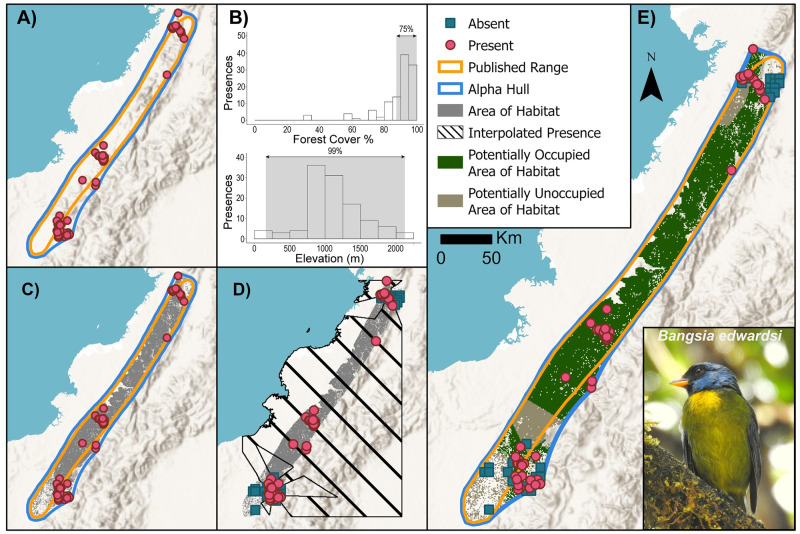
We created an alpha hull around the union of the range map vertices and the eBird presence points (Fig 1A) using the ‘alphahull’ package [15]. These alpha hulls “pinch in” the boundaries from a minimum convex polygon, thereby providing a more conservative range boundary. It is more tightly fitted to the underlying data, particularly where a species has a curved distribution, such as a species occurring along the Andes. The alpha value controls the degree of “pinching”. Infinite alphas result in a shape identical to a minimum convex polygon while very small alphas result in a polygon for each point. For our methods, we use the median inter-presence distance as the alpha value for each species. Therefore, if the points are evenly distributed, the resulting alpha hull will be a single polygon. If the point data are clustered, the resulting alpha hull will split into multiple polygons.

To create an estimate of elevational range for each species, we calculated the distribution of elevations at the presence points using the GLOBE 1 km digital elevation model [16]. To restrict the impact of outliers, we excluded the highest and lowest 1% of the elevation estimates. Inspection of eBird data along with personal experience suggests that some reported locations may be a convenient landmark, such as a nearby peak, settlement, or lake, which can thereby bias the elevational range. We then compared the 1^st and 99^th percentiles with the documented elevation preferences in the IUCN Red List assessment. We used the smaller of the calculated GLOBE and documented Red List elevations as the minimum and the larger of the GLOBE and Red List elevations as the maximum to determine the final elevational range of the species.

We created the habitat layer using the 30 m Hansen et al. forest cover dataset [17] bilinearly resampled to 1 km. We extracted the tree cover percentage for every observation from 2000 onward within a 1 km × 1km cell. We excluded all occurrences falling within 0% of tree cover as these observations weighted negatively for forest species and often represented lodges or trailheads rather than the specific location of observation. Using the distribution of tree cover values, we defined the habitat range as the upper 75% of the observed values. This criterion excluded unusually low values that often represent settlements below the actual location of the bird (Fig 1B). It should also be noted that the Hansen et al. forest cover data include plantations, which may be unsuitable habitat for some species. Unsurprisingly, our estimates of Area of Habitat are only as good as the quality of the habitat data. Future efforts could incorporate more accurate habitat data or utilise data on other habitat types to map more species.

We calculate Area of Habitat from the intersection between the elevational and forest layers within the alpha hull (Fig 1C). We then refined the Area of Habitat into Potentially Occupied Area of Habitat and Potentially Unoccupied Area of Habitat using a nearest-neighbour interpolation between presences and absences. We define absences as 5km × 5km grid cells that are surveyed with 25 or more complete checklists and no presences of the species of concern within the cell. When calculating these absences, we filtered the checklist data to keep only those that fall within pixels of the Area of Habitat. Thus, if a checklist falls in a location that is deemed to be inappropriate in terms of elevation or land cover, it is not counted towards the threshold for being absent, as one would not expect to find the species in unsuitable habitat. This choice differs from what we defined for presences, where all were retained even if they fall outside what we previously calculated as Area of Habitat. This was to allow for some approximation of recording a presence while we do not expect species to be recorded in checklists in unsuitable habitat. We used the centre of each absence cell for the interpolation (Fig 1D and 1E). For the final step, we compiled all layers and created the interactive HTML maps using the ‘leaflet’ package [18].

eBird Historical and Incidental, and GBIF

For comparison purposes and to evaluate the potential of incorporating more data, we included Historical and Incidental eBird records as well as data from Global Biodiversity Information Facility (GBIF, www.gbif.org), which include observations from iNaturalist (www.inaturalist.org). These data are displayed on the interactive maps, though we do not calculate ranges using these data. For GBIF data, we applied a strict filtering process to remove all locations with issues associated with geolocation and missing coordinates. We retained records with “Rounded Coordinate” since that did not impact our confidence in those points. We removed all eBird records from the GBIF dataset to avoid redundancy.

Results

We mapped the Area of Habitat for the 1,151 terrestrial bird species that have breeding and resident ranges from Mexico southwards. Of these, we are not confident in our estimates for 99 species that had fewer than 10 observation and for 92 desert, grassland, and shrubland species, given challenges in mapping these habitats.

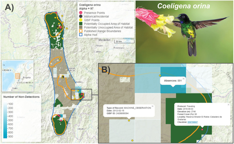
Fig 2 shows an exemplar map for a hummingbird, the glittering starfrontlet, Coeligena orina (Endangered). This species has a small range in the Western Andes of Colombia, west of Medellin. We map Area of Habitat, dividing it into Potentially Occupied Area of Habitat in dark green—these are cells nearer to sightings of the species—and Potentially Unoccupied Area of Habitat in brown—cells nearer to where observers have repeatedly not recorded the species. Some of the latter areas are consistently well surveyed without recording a presence, while others may represent a call for more exploration.

Unsurprisingly, estimates of Area of Habitat and Potentially Occupied Area of Habitat correlate positively with the extent of published ranges (Fig 3). As one might expect, estimates based on fewer than ten observations often relate to species with small ranges. They show a wider scatter, reflecting the small sample size. The outliers—either those with larger areas of habitat or smaller—suggest that re-evaluation of published ranges is warranted.

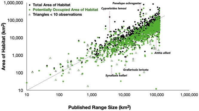
Fig 3 — Black symbols represent estimates of total Area of Habitat and green symbols represent Potentially Occupied Area of Habitat. Solid symbols represent species with ten or more observations, open triangles represent those with fewer than ten. The text discusses the five examples labelled. Dotted diagonal line shows identical values along the two axes.

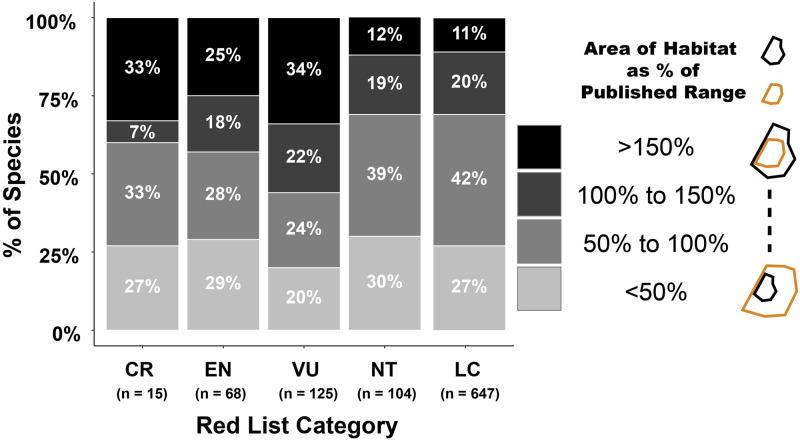
Although correlated, the relationship between the area of published ranges and our estimates of Area of Habitat varies widely (Fig 4). Across all forest species analysed, our estimates of Area of Habitat were on average 12% larger (σ = 185%) than the published ranges (S1 Table). Our estimates of Potentially Occupied Area of Habitat were on average 70% of the areas of published range (σ = 93%). Among threatened species (Vulnerable, Endangered, and Critically Endangered, n = 208), 24% have Areas of Habitat <50% of the published ranges due to lack of suitable habitat within the range. These proportions of species with Area of Habitat <50% of range are similar for Near Threatened (30%) and Least Concern (27%) species. Meanwhile, 31% of threatened species have Areas of Habitat >150% of the published ranges because eBird observations expand the range boundary beyond the published ranges. By contrast, the equivalent proportions are much smaller for Near Threatened (12%) and Least Concern (11%) species with Area of Habitat >150% of the published ranges. Such instances suggest that the species may be more widespread than previously recognised. Our approach facilitates checking of observations that expand known range and encourages their confirmation.

For some species, the published ranges include locations in which there are no eBird data (neither recorded presences nor absences inferred from complete checklists omitting the species). These may derive from information from remote areas that are inaccessible to most eBird observers (e.g., owing to current security concerns) or from areas that historical ornithological expeditions visited. These cases call for further research and exploration of the areas in search of the species. Alternatively, they may represent errors in the boundaries of published ranges or unoccupied areas within the species’ distributional limits. (The range maps represent range boundaries rather than occupancy.) In many cases, we found areas within the alpha hull boundary (whether within the published range or not), where there are no records, but which nonetheless have forest cover within the elevation range that may support the species.

Species for which Area of Habitat is greater than published range

Crowd-sourced data expanded the range boundaries of some species considerably (Fig 3). An extreme example is the white-chested swift, Cypseloides lemosi (Vulnerable). Known to science only since 1962 and then from the upper Cauca Valley in Central Colombia—which the published range represents—eBird records show it to occur widely in Colombia, Ecuador, Peru, and into Bolivia. For this species, we estimated an Area of Habitat that is >40 times the published range size.

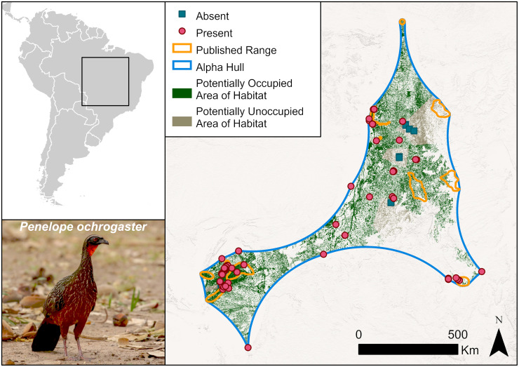
A second example is the chestnut-bellied guan, Penelope ochrogaster (Vulnerable) (Figs 3 and 5). The published range represents ten or so scattered locations in south-east Amazonia, while eBird records indicate a more continuous distribution.

Fig 5 — eBird records illustrate that the range of P. *ochrogaster* expands beyond the published range. Symbology is simplified to show absences (blues squares) as the centroids of absence grid cells. Base map provided by USGS and photo by Carlos Sanchez with permission.

We analysed 208 species listed as threatened. For 64 of these, our estimates of the Area of Habitat are >150% of the published ranges (Fig 4 and S1 Table). That crowd-sourced data considerably expand these published ranges need not necessarily change their Red List category. For example, some large-ranged species are listed as threatened owing to rapid rates of decline. Examples include various parrot species trapped for the pet trade and guan and curassow species that are heavily hunted. Other species with large published ranges may have small populations because their ranges are exceptionally fragmented [19, 20], or because the species occurs at naturally low densities. Nonetheless, some of these species may prove to be less threatened than currently considered.

Species for which Area of Habitat is smaller than published range

Of potential conservation concern are those species that have an Area of Habitat much smaller than the published range. A disadvantage of using polygons to map species distributions is that they mask areas lacking habitat within the range boundaries, often prevalent in regions experiencing rapid land cover changes. Lack of understanding of habitat distribution may lead to over-estimating population sizes (or underestimating decline rates) and hence underestimating the extinction risk of such species.

An extreme example is the hoary-throated spinetail, Synallaxis kollari (Critically Endangered) which has an Area of Habitat of only 6% of the published range (Fig 3 and S1 Table). It lives in narrow gallery forests along rivers in northern Brazil that transit areas that are otherwise grasslands [21]. Agricultural expansion threatens the remaining habitat. Dependence on forests explains its small Area of Habitat and points to the limitation of creating simple polygons to describe ranges. Only a much finer, more convoluted polygon would describe this range more accurately.

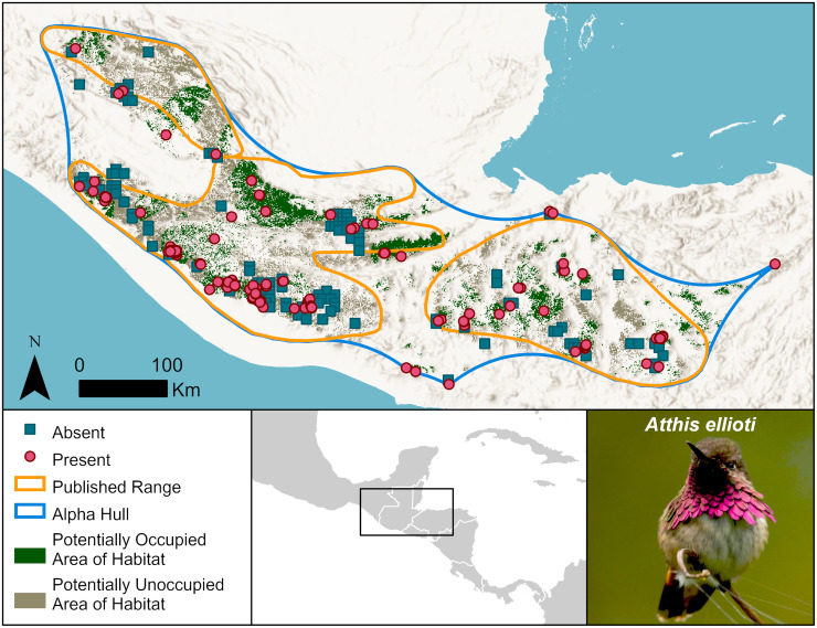
Two more examples are from Central America: the wine-throated hummingbird, Atthis ellioti (Least Concern) (Figs 3 and 6), and the black-throated jay, Cyanolyca pumilio (Least Concern). Both are listed as Least Concern because of their large Extent of Occurrence and inferred population sizes and lack of rapid population declines. The hummingbird has a published range of 94,985 km². eBird observations extend beyond its published range substantially south to mountains in El Salvador and well to the east in Honduras, yet we estimate the species’ Area of Habitat at only 25,804 km², falling to 12,594 km² if we consider only Potentially Occupied Area of Habitat. The black-throated jay resides in a highly fragmented landscape [22]. We estimate its Area of Habitat as 21,421 km² while its published range is 103,160 km². While the Extent of Occurrence for both species exceed the thresholds to trigger assessment as a threatened species, extensive and continuing deforestation leaves the remaining forests where these species occur in widely isolated fragments. These facts suggest the importance of careful monitoring of possible threats to these species is needed.

Fig 6 — The published range boundaries are large, but extensive deforestation has left the remaining forests few and fragmented, resulting in a much smaller Area of Habitat. Symbology is simplified to show absences (blues squares) as the centroids of absence grid cells. Basemap provided by USGS and photo provided by David Mora Vargas (Macaulay Library, ML296645721).

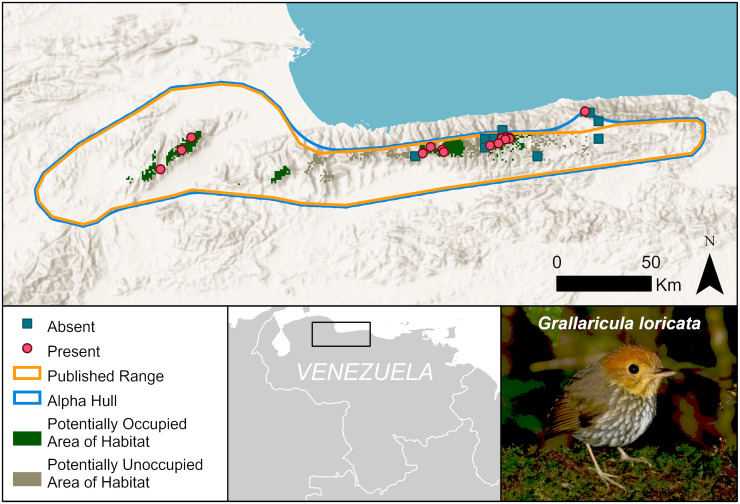
A final example is the scallop-breasted antpitta, Grallaricula loricata (Near Threatened) (Figs 3 and 7). We estimate an Area of Habitat to be only 447 km² in several widely separated forest patches. The new mapped distribution of this species may inform future reassessment of whether more than half the population occurs in small and isolated subpopulations (i.e. ‘‘severely fragmented”) or within fewer than 10 locations (as defined by threats, following the definitions of IUCN [3].

Fig 7 — Due to habitat loss and restricted elevational range, the Area of Habitat is much smaller than the current published range size. Symbology is simplified to show absences (blues squares) as the centroids of absence grid cells. Basemap provided by USGS and photo provided by Margareta Wieser (Macaulay Library, ML205392301).

Discussion

General findings

Previous estimates of Areas of Habitat were constrained within the published ranges and thus were, by definition, smaller—typically about 30% [6]. This reflects how little habitat within suitable elevation ranges exists within those published ranges for the species. Our results show that on average, Areas of Habitat are 12% larger than published ranges, reflecting the often-considerable extent that eBird records expand the known distributions of species beyond published ranges.

Interestingly, there are substantial differences between threatened and non-threatened species. Some 40% of Critically Endangered, 43% of Endangered, and 55% of Vulnerable species have Areas of Habitat larger than their published ranges, compared with 31% for Near Threatened and Least Concern species (Fig 4). This may be because non-threatened species are better known, more common, and have generally larger ranges than the threatened species. Alternatively, threatened species, particularly those with small ranges, may have been mapped at finer resolution than non-threatened species, i.e. their range boundaries have been delineated to exclude areas in which the species in absent, whereas those of non-threatened species are cruder approximations of the range limits. The important finding for conservation is that threatened species are generally more widespread than previously estimated.

Advantages

Transparency

The maps are explicit about what we know and what we do not. They predict Areas of Habitat where we expect the species to live but in which observers have not recorded it in eBird. They also predict areas within existing range maps where a species is unlikely to live because the elevations or habitat are outside its known preferences. For instance, in some areas within Central America (Fig 6), what habitat remains is massively fragmented, posing additional risk to species over and above the simple habitat loss [19, 20]. eBird’s data collection protocols, which by requiring observers to document whether or not every bird recorded is included in a checklist, allow assessment of absence and presence, and thus innovation to differentiate between Potentially Occupied Area of Habitat and Potentially Unoccupied Area of Habitat. Development and application of similar techniques for assessing absence using other crowd-sourced species datasets, such as iNaturalist, would be necessary to enable the extension of this innovation to taxa other than birds.

Our maps predict where further exploration would be prudent. Birdwatchers tend to visit known sites for particularly rare species, rather than explore new ones, to the detriment of modelling species ranges [23]. (Of course, in seeking rarities, they also document other species coincidentally.) Our maps also predict where the species might occur, but nearby surveys have not found it, thereby hopefully encouraging further exploration.

Provenance

Interactive maps permit users to interrogate the provenance of observations by querying individual records to check their likely validity. Without provenance, we cannot understand how maps are produced and what might be their limitations. Users can interpret that information as they see fit.

Revision

By design, we developed the methods herein to enable users to update maps at regular intervals as observations accumulate and forest cover changes. The methods can include other sources of records. We can explore how eBird data availability alters our maps, either through growth in the dataset over time or through analysing subsets or supersets of the data.

In addition, as further context, our maps display data from GBIF and historical observations from eBird that we did not use to calculate Areas of Habitat. Inspection of those data may suggest locations where species are unlikely to occur now because no habitat remains. Our maps afford the chance to study the changes in Areas of Habitat that have occurred and will likely occur in the future.

Limitations

High elevation, desert, and other open land species

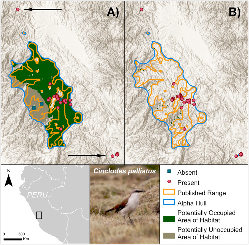
Given the habitat data we used, we were not confident in mapping Area of Habitat for 92 non-forest species (S1 Table). We checked these individually against the species’ known elevations and habitat preferences and excluded them from the statistical summaries. Nonetheless, eBird observations may still yet expand the species’ range beyond what is currently published. One such example is the white-bellied cinclodes, Cinclodes palliatus, an open area species that is Critically Endangered owing to small and declining populations. For such species, we can produce maps limited by elevation, but not habitat (Fig 8). These elevation-only maps often appear very similar to the published ranges. Although accessible, high-resolution vegetation datasets are predominantly available for forest habitat, our method has the potential to be expanded to other habitats when appropriate datasets become available. At present, we have not extended our approach to other habitats by matching landcover classes at points where eBird observations fall to habitat classes as coded on the IUCN Red List owing to errors of omission and commission in such matches.

Fig 8 — (A) Estimates of Area of Habitat for species that prefer open land are often similar to the published ranges when refined just by the estimated elevational ranges. (B) Further refining a species range using forest cover—not a preferred habitat—may lead to a significant underestimation of Area of Habitat. Despite lack of appropriate landcover data to refine Area of Habitat, eBird records beyond the published range (identified with arrows) inform us that the range of these species is wider than recognised. Symbology is simplified to show absences (blues squares) as the centroids of absence grid cells. Basemaps provided by USGS and photos provided by Stuart Pimm with permission.

Other habitat specialists

Some species specialise on narrow or monodominant vegetation types within forest but not distinguished by our forest cover data. Our Area of Habitat estimates are likely too extensive for these species, and additional analyses will be needed to estimate them more precisely (see S1 Text for a more detailed discussion). These include many bamboo habitat specialists [24–26], some of which are nomadic, depending on periodic mass seeding events, a strategy that may have doomed the purple-winged ground dove, Paraclaravis geoffroyi (Critically Endangered), to extinction. Its published range is nearly half a million square kilometres—the range over which it searched for seeding bamboo.

Some 7% of the Amazon Basin consists of white-sand ecosystems [27]. Together with other forest types limited to nutrient-poor soils, this ecosystem harbours many habitat specialists. Other species within the Amazon Basin are restricted to floodplain forests; examples include the wattled curassow, Crax globulosa (Endangered), and the pearly-breasted conebill, Conirostrum margaritae (Vulnerable). Mangrove specialists such as the mangrove hummingbird, Amazilia boucardi (Endangered), may pose a challenge because some landcover datasets do not differentiate mangroves and adjacent moist forests [28, 29].

Intra-tropical migratory birds

Although most of the species we analyse are mainly resident birds, some species (e.g., swifts, hummingbirds, and songbirds) make regular but poorly understood movements and migrations across altitudinal and wet-dry gradients. Likewise, some species are more prone to vagrancy than others, including Andean species that might occasionally descend to the lower elevations or even the lowlands as a temporary escape from harsh weather. Different mapping methods are required to distinguish breeding habitat from other habitats for these species.

Introduced species

eBird records include species outside their native range. For example, most eBird records of the red-crowned amazon, Amazona viridigenalis (Endangered) are from southern California, where it is introduced, and southern Texas, where it may be a colonist. Fewer observations exist in its known native range in Mexico, a fact evident for this species, but not always so for other introduced species.

Taxonomic issues

eBird and BirdLife International are working towards, but have not yet completed, a common taxonomy. Even a taxon as well-known as birds generates taxonomic debates, often prompted by improving knowledge. Debates among taxonomists will never disappear entirely, but the maps we produce can, nonetheless, provide useful insights into the issues.

Some differences merely involve different generic names. For 135 species in our sample, however, the issue is that Handbook of the Birds of the and BirdLife International [1] split out what eBird considers to be subspecies. Many occur in the Andes where the topography isolates montane taxa into separate populations. An example is the violet-throated starfrontlet, Coeligena violifer (Least Concern), which eBird considers to be one species but [1] treats as four separate species, splitting out C. dichroura (Least Concern), C. albicaudata (Least Concern), and C. osculans (Least Concern).

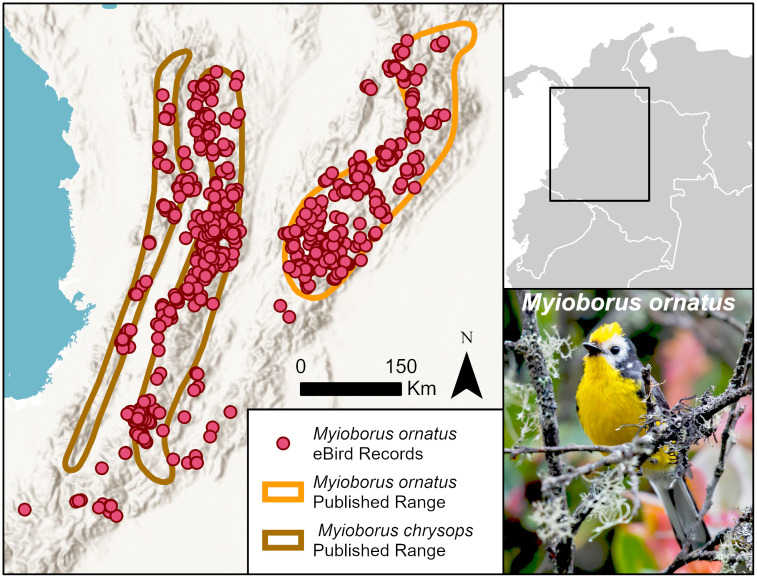
This easy separation is not always the case, whereupon eBird observations afford insights for how taxonomists might draw their conclusions. An example is the golden-fronted redstart, which [1] considers to be two species: yellow fronted redstart, Myioborus ornatus (Least Concern), and golden-fronted redstart, Myioborus chrysops (Least Concern) (Fig 9). The numerous eBird observations cluster into three separate mountain ranges in Colombia—the Western, Central, and Eastern Andes, but extend much further south in the last two ranges than the published ranges suggest. Analysis of the genetics of this species group would likely be informative.

Fig 9 — eBird considers *Myioborus ornatus* to be one species, but [1] treat it as two separate species: *Myioborus ornatus* in the Eastern Andes (orange polygon) and *Myioborus chrysops* in the Central and Western Andes (brown polygon). Basemap provided by USGS and photo provided by Juan José Arango with permission.

Of greatest concern from a conservation standpoint are species that, when split, are assessed as threatened on the IUCN Red List. Due to difficulties in assigning eBird records to the appropriate taxon, we were unable to produce maps for two such threatened species: the lilacine amazon, Amazona lilacina (Critically Endangered), and the white-tailed canastero, Asthenes usheri (Vulnerable).

Methodological decisions

Our methods include various decisions, including how we filter observations, the use of alpha-hulls and their parameterization, the selection of elevational limits, the grain of the elevation maps, the forest cover limits and others. All are arbitrary and the choices we make are motivated by pragmatism. We explored some of their consequences in the supplementary materials. Estimates of the elevational range for instance, may be dependent on the DEM resolution one uses in conjunction with eBird data. Therefore, taking the union with previously published range estimates is the more conservative solution. Importantly, because our methods are transparent and the maps we produce allow one to interrogate each datum, one can readily explore the consequences of the decisions we have made.

Conclusions

We present a novel and transparent approach to mapping and updating range maps for birds using crowd-sourced observation data and spatial elevation and land cover information. These maps, and the method used to produce them, are freely available, so that the maps can be periodically updated based on new observation and habitat data. The utility of these maps is broad, providing a basis for potentially evaluating species’ natural history, extinction risk, habitat threats, and conservation priorities.

This paper’s authors include representatives from the IUCN and BirdLife International (Red List Authority for birds, and hence responsible for their Red List assessments, including the production of maps of current ranges). Authors from American Bird Conservancy (www.abcbirds.org) and Saving Nature (www.savingnature.org) help acquire land for protection based on where threatened species live, hence depend on the best possible maps to identify priorities. Also represented is the Cornell Lab of Ornithology eBird team (www.ebird.org), an organization that has archived a billion crowd-sourced observations of birds globally. Lastly, included is a community of scientific users interested in bringing the rapidly expanding GIS data to bear on species mapping problems.

The maps produced inform the needs of these various constituencies, being transparent in the provenance of their data, straightforward to update when needed, and feasibly aggregated to identify areas of conservation concern and, as above, areas where further exploration would be helpful.

Supporting information

Each species’ mapped elevation ranges, forest cover thresholds, major habitat requirements, Area of Habitat estimates, published range sizes, and IUCN Red List category are given in S1 Table. The supplementary materials provides an extended technical description of methodology for combining published data on geographical ranges, elevations, and habitat preferences with crowd-sourced data. S2 Table provides a detail set of estimated elevational ranges of species. Additionally, we supply code in R for the algorithm described in the Methods.

S1 Text. Analysis and discussion of methodological choices on results.

(DOCX)

Click here for additional data file.^{(899.7KB, docx)}

S1 Code. Detailed description and full code base for reproducing methods.

(PDF)

Click here for additional data file.^{(1.1MB, pdf)}

S1 Table. Summary table of species analyzed.

Table detailing all target species identified, reason for exclusion from the analysis (if any) and all relevant metrics.

(XLSX)

Click here for additional data file.^{(236.6KB, xlsx)}

S2 Table. Summary table of elevational estimates.

Table of elevational estimates derived from BirdLife, Stotz et al. (1996), or from crowd-source data overlaid on either 90m or 1km DEM.

(XLSX)

Click here for additional data file.^{(279.3KB, xlsx)}

S3 Table. Effects of elevational estimates on Area of Habitat.

Comparison of using different estimates of elevational range in calculating Area of Habitat for the eight species with the largest discrepancies.

(XLSX)

Click here for additional data file.^{(15.9KB, xlsx)}

Acknowledgments

We would like to thank the community of eBird users who have contributed data, without which this work would not be possible, and the large number of contributors to BirdLife’s Red List assessments (including range maps) for all birds. The first generation of maps may be viewed at https://osf.io/snmk4/.

Data Availability

The data is now hosted in an approved data repository (OSF) and the updated link is provided in the Acknowledgements: (https://osf.io/snmk4/).

Funding Statement

The authors thank their home institutions for providing support.

References

1.Handbook of the Birds of the World and BirdLife International. Handbook of the Birds of the World and BirdLife International digital checklist of the birds of the world. Version 4. http://datazone.birdlife.org/userfiles/file/Species/Taxonomy/HBW-BirdLife_Checklist_v5_Dec20.zip. 2019.
2.Manne LL, Brooks TM, Pimm SL. Relative risk of extinction of passerine birds on continents and islands. Nature. 1999;399(6733):258–61. [Google Scholar]
3.IUCN. The IUCN Red List of Threatened Species; www.iucnredlist.org. 2021.
4.Brooks TM, Pimm SL, Akçakaya HR, Buchanan GM, Butchart SH, Foden W, et al. Measuring terrestrial area of habitat (AOH) and its utility for the IUCN Red List. Trends in ecology & evolution. 2019;34(11):977–86. [DOI] [PubMed] [Google Scholar]
5.Ocampo-Peñuela N, Jenkins CN, Vijay V, Li BV, Pimm SL. Incorporating explicit geospatial data shows more species at risk of extinction than the current Red List. Science Advances. 2016;2(11):e1601367. doi: 10.1126/sciadv.1601367 [DOI] [PMC free article] [PubMed] [Google Scholar]
6.Li BV, Hughes AC, Jenkins CN, Ocampo-Peñuela N, Pimm SL. Remotely sensed data informs Red List evaluations and conservation priorities in Southeast Asia. PloS one. 2016;11(8):e0160566. [DOI] [PMC free article] [PubMed] [Google Scholar]
7.Pimm SL, Jenkins CN, Abell R, Brooks TM, Gittleman JL, Joppa LN, et al. The biodiversity of species and their rates of extinction, distribution, and protection. science. 2014;344(6187). [DOI] [PubMed] [Google Scholar]
8.Haddad NM, Brudvig LA, Clobert J, Davies KF, Gonzalez A, Holt RD, et al. Habitat fragmentation and its lasting impact on Earth’s ecosystems. Science advances. 2015;1(2):e1500052. doi: 10.1126/sciadv.1500052 [DOI] [PMC free article] [PubMed] [Google Scholar]
9.Gu W, Swihart RK. Absent or undetected? Effects of non-detection of species occurrence on wildlife–habitat models. Biological Conservation. 2004;116(2):195–203. [Google Scholar]
10.Sullivan BL, Aycrigg JL, Barry JH, Bonney RE, Bruns N, Cooper CB, et al. The eBird enterprise: an integrated approach to development and application of citizen science. Biological Conservation. 2014;169:31–40. [Google Scholar]
11.BirdLife_International. Bird species distribution maps of the world. Version 2019.1. http://datazonebirdlifeorg/species/requestdis. 2019.
12.Clements J, Schulenberg T, Iliff M, Roberson D, Fredericks T, Sullivan B, et al. The eBird/Clements checklist of birds of the world: v2016. Extraído el. 2018;31(12):2018. [Google Scholar]
13.Strimas-Mackey M, Miller E, Hochachka W. auk: eBird Data Extraction and Processing with AWK. R package version. 2017.
14.Johnston A, Hochachka WM, Strimas‐Mackey ME, Ruiz Gutierrez V, Robinson OJ, Miller ET, et al. Analytical guidelines to increase the value of community science data: An example using eBird data to estimate species distributions. Diversity and Distributions. 2021. [Google Scholar]
15.Pateiro-Lopez B, Rodriguez-Casal A. alphahull: Generalization of the Convex Hull of a Sample of Points in the Plane, 2016. R package version. 2.
16.Team GT, Hastings D, Dunbar P, Elphingstone G, Bootz M, Murakami H, et al. The Global Land One-kilometer Base Elevation (GLOBE) Digital Elevation Model. 1998. [Google Scholar]
17.Hansen MC, Potapov PV, Moore R, Hancher M, Turubanova SA, Tyukavina A, et al. High-resolution global maps of 21st-century forest cover change. science. 2013;342(6160):850–3. doi: 10.1126/science.1244693 [DOI] [PubMed] [Google Scholar]
18.Cheng J, Karambelkar, Bhaskar, Xie, Yihui. leaflet: Create Interactive Web Maps with the JavaScript ’Leaflet’ Library. R package version 2.0.4.1. https://CRAN.R-project.org/package=leaflet. 2021.
19.Schnell JK, Harris GM, Pimm SL, Russell GJ. Quantitative analysis of forest fragmentation in the Atlantic Forest reveals more threatened bird species than the current Red List. PLoS One. 2013;8(5):e65357. doi: 10.1371/journal.pone.0065357 [DOI] [PMC free article] [PubMed] [Google Scholar]
20.Schnell JK, Harris GM, Pimm SL, Russell GJ. Estimating extinction risk with metapopulation models of large‐scale fragmentation. Conservation Biology. 2013;27(3):520–30. doi: 10.1111/cobi.12047 [DOI] [PubMed] [Google Scholar]
21.Vale MM, Bell JB, Alves MAS, Pimm SL. Abundance, distribution and conservation of Rio Branco Antbird Cercomacra carbonaria and Hoary-throated Spinetail Synallaxis kollari. Bird Conservation International. 2007;17(3):245–57. [Google Scholar]
22.Harris G, Pimm SL. Range size and extinction risk in forest birds. Conservation Biology. 2008;22(1):163–71. doi: 10.1111/j.1523-1739.2007.00798.x [DOI] [PubMed] [Google Scholar]
23.Pimm SL, Harris G, Jenkins CN, Ocampo‐Peñuela N, Li BV. Unfulfilled promise of data‐driven approaches: response to Peterson et al. Conservation Biology. 2017;31(4):944–7. doi: 10.1111/cobi.12928 [DOI] [PubMed] [Google Scholar]
24.Kratter AW. Bamboo Specialization by Amazonian Birds 1. Biotropica. 1997;29(1):100–10. [Google Scholar]
25.Areta JI, Cockle KL. A theoretical framework for understanding the ecology and conservation of bamboo-specialist birds. Journal of Ornithology. 2012;153(1):163–70. [Google Scholar]
26.Lebbin DJ. Nestedness and Patch Size of Bamboo-Specialist Bird Communities in Southeastern Peru: Anidamiento y Tamaño de Parche en Comunidades de Aves Especialistas de Bambú en el Sudeste de Perú. The Condor. 2013;115(2):230–6. [Google Scholar]
27.Adeney JM, Christensen NL, Vicentini A, Cohn‐Haft M. White‐sand ecosystems in Amazonia. Biotropica. 2016;48(1):7–23. [Google Scholar]
28.Huang R, Pimm SL, Giri C. Using metapopulation theory for practical conservation of mangrove endemic birds. Conservation Biology. 2020;34(1):266–75. doi: 10.1111/cobi.13364 [DOI] [PMC free article] [PubMed] [Google Scholar]
29.Giri C, Ochieng E, Tieszen LL, Zhu Z, Singh A, Loveland T, et al. Status and distribution of mangrove forests of the world using earth observation satellite data. Global Ecology and Biogeography. 2011;20(1):154–9. [Google Scholar]

PLoS One. doi: 10.1371/journal.pone.0259299.r001

Decision Letter 0

Tim A Mousseau

28 Sep 2021

PONE-D-21-23994Batch-produced, GIS-informed range maps for birds based on provenanced, crowd-sourced data inform conservation assessmentsPLOS ONE

Dear Stuart,

At long last, both reviews are in! Congratulations! Both the reviewers and I strongly feel this represents a very valuable (and useful) addition to the literature. However, there were a few small suggestions that probably should be tended to. Hence the "minor revision". But these are largely cosmetic and should not cause too much grief. Therefore, we invite you to submit a revised version of the manuscript that addresses the points raised during the review process.

Please submit your revised manuscript by Nov 12 2021 11:59PM. If you will need more time than this to complete your revisions, please reply to this message or contact the journal office at plosone@plos.org. When you're ready to submit your revision, log on to https://www.editorialmanager.com/pone/ and select the 'Submissions Needing Revision' folder to locate your manuscript file.

Please include the following items when submitting your revised manuscript:

A rebuttal letter that responds to each point raised by the academic editor and reviewer(s). You should upload this letter as a separate file labeled 'Response to Reviewers'.
A marked-up copy of your manuscript that highlights changes made to the original version. You should upload this as a separate file labeled 'Revised Manuscript with Track Changes'.
An unmarked version of your revised paper without tracked changes. You should upload this as a separate file labeled 'Manuscript'.

If you would like to make changes to your financial disclosure, please include your updated statement in your cover letter. Guidelines for resubmitting your figure files are available below the reviewer comments at the end of this letter.

If applicable, we recommend that you deposit your laboratory protocols in protocols.io to enhance the reproducibility of your results. Protocols.io assigns your protocol its own identifier (DOI) so that it can be cited independently in the future. For instructions see: https://journals.plos.org/plosone/s/submission-guidelines#loc-laboratory-protocols. Additionally, PLOS ONE offers an option for publishing peer-reviewed Lab Protocol articles, which describe protocols hosted on protocols.io. Read more information on sharing protocols at https://plos.org/protocols?utm_medium=editorial-email&utm_source=authorletters&utm_campaign=protocols.

We look forward to receiving your revised manuscript.

Kind regards,

Tim A. Mousseau

Academic Editor

PLOS ONE

Journal Requirements:

When submitting your revision, we need you to address these additional requirements.

1. Please ensure that your manuscript meets PLOS ONE's style requirements, including those for file naming. The PLOS ONE style templates can be found at

https://journals.plos.org/plosone/s/file?id=wjVg/PLOSOne_formatting_sample_main_body.pdf and

https://journals.plos.org/plosone/s/file?id=ba62/PLOSOne_formatting_sample_title_authors_affiliations.pdf

2. We note that Figure(s) 1 , in your submission contain [map/satellite] images which may be copyrighted. All PLOS content is published under the Creative Commons Attribution License (CC BY 4.0), which means that the manuscript, images, and Supporting Information files will be freely available online, and any third party is permitted to access, download, copy, distribute, and use these materials in any way, even commercially, with proper attribution. For these reasons, we cannot publish previously copyrighted maps or satellite images created using proprietary data, such as Google software (Google Maps, Street View, and Earth). For more information, see our copyright guidelines: http://journals.plos.org/plosone/s/licenses-and-copyright.

We require you to either (1) present written permission from the copyright holder to publish these figures specifically under the CC BY 4.0 license, or (2) remove the figures from your submission:

1. You may seek permission from the original copyright holder of Figure(s) [#] to publish the content specifically under the CC BY 4.0 license.

We recommend that you contact the original copyright holder with the Content Permission Form (http://journals.plos.org/plosone/s/file?id=7c09/content-permission-form.pdf) and the following text:

“I request permission for the open-access journal PLOS ONE to publish XXX under the Creative Commons Attribution License (CCAL) CC BY 4.0 (http://creativecommons.org/licenses/by/4.0/). Please be aware that this license allows unrestricted use and distribution, even commercially, by third parties. Please reply and provide explicit written permission to publish XXX under a CC BY license and complete the attached form.”

Please upload the completed Content Permission Form or other proof of granted permissions as an "Other" file with your submission.

In the figure caption of the copyrighted figure, please include the following text: “Reprinted from [ref] under a CC BY license, with permission from [name of publisher], original copyright [original copyright year].”

2. If you are unable to obtain permission from the original copyright holder to publish these figures under the CC BY 4.0 license or if the copyright holder’s requirements are incompatible with the CC BY 4.0 license, please either i) remove the figure or ii) supply a replacement figure that complies with the CC BY 4.0 license. Please check copyright information on all replacement figures and update the figure caption with source information. If applicable, please specify in the figure caption text when a figure is similar but not identical to the original image and is therefore for illustrative purposes only.

The following resources for replacing copyrighted map figures may be helpful:

USGS National Map Viewer (public domain): http://viewer.nationalmap.gov/viewer/

The Gateway to Astronaut Photography of Earth (public domain): http://eol.jsc.nasa.gov/sseop/clickmap/

Maps at the CIA (public domain): https://www.cia.gov/library/publications/the-world-factbook/index.html and https://www.cia.gov/library/publications/cia-maps-publications/index.html

NASA Earth Observatory (public domain): http://earthobservatory.nasa.gov/

Landsat: http://landsat.visibleearth.nasa.gov/

USGS EROS (Earth Resources Observatory and Science (EROS) Center) (public domain): http://eros.usgs.gov/#

Natural Earth (public domain): http://www.naturalearthdata.com/

3. Thank you for stating the following in the Acknowledgments Section of your manuscript:

"Funding: The authors thank their home institutions for providing support"

We note that you have provided funding information that is not currently declared in your Funding Statement. However, funding information should not appear in the Acknowledgments section or other areas of your manuscript. We will only publish funding information present in the Funding Statement section of the online submission form.

Please remove any funding-related text from the manuscript and let us know how you would like to update your Funding Statement. Currently, your Funding Statement reads as follows:

"The authors thank their home institutions for providing support"

Please include your amended statements within your cover letter; we will change the online submission form on your behalf

Please review your reference list to ensure that it is complete and correct. If you have cited papers that have been retracted, please include the rationale for doing so in the manuscript text, or remove these references and replace them with relevant current references. Any changes to the reference list should be mentioned in the rebuttal letter that accompanies your revised manuscript. If you need to cite a retracted article, indicate the article’s retracted status in the References list and also include a citation and full reference for the retraction notice.

[Note: HTML markup is below. Please do not edit.]

Reviewers' comments:

Reviewer's Responses to Questions

Comments to the Author

1. Is the manuscript technically sound, and do the data support the conclusions?

The manuscript must describe a technically sound piece of scientific research with data that supports the conclusions. Experiments must have been conducted rigorously, with appropriate controls, replication, and sample sizes. The conclusions must be drawn appropriately based on the data presented.

Reviewer #1: Yes

Reviewer #2: Yes

**********

2. Has the statistical analysis been performed appropriately and rigorously?

Reviewer #1: Yes

Reviewer #2: Yes

**********

3. Have the authors made all data underlying the findings in their manuscript fully available?

The PLOS Data policy requires authors to make all data underlying the findings described in their manuscript fully available without restriction, with rare exception (please refer to the Data Availability Statement in the manuscript PDF file). The data should be provided as part of the manuscript or its supporting information, or deposited to a public repository. For example, in addition to summary statistics, the data points behind means, medians and variance measures should be available. If there are restrictions on publicly sharing data—e.g. participant privacy or use of data from a third party—those must be specified.

Reviewer #1: Yes

Reviewer #2: Yes

**********

4. Is the manuscript presented in an intelligible fashion and written in standard English?

PLOS ONE does not copyedit accepted manuscripts, so the language in submitted articles must be clear, correct, and unambiguous. Any typographical or grammatical errors should be corrected at revision, so please note any specific errors here.

Reviewer #1: Yes

Reviewer #2: Yes

**********

5. Review Comments to the Author

Please use the space provided to explain your answers to the questions above. You may also include additional comments for the author, including concerns about dual publication, research ethics, or publication ethics. (Please upload your review as an attachment if it exceeds 20,000 characters)

Reviewer #1: The authors of this manuscript have produced a useful tool for generating provenanced range maps so that they can be used to inform conservation assessments. However, despite the apparent utility of the tool to batch process large numbers of species, the authors repeatedly mention the need for closer inspection of the data in order to filter out incorrect records. The title and the abstract both emphasise the batch processing aspects, but much of the main text refers to the need for careful inspection of the data, so it is not clear how much of the process is automated and how much additional time is needed to manually correct data. It would be good of the authors could provide some estimates of how much time it takes to collate the data sets, how long it takes the protocol to do the batch processing, and how much time has to be spent manually checking and correcting data.

The authors do admit to the concerns about the quality and reliability of the eBird data (lines 102-107) and explain that the protocol does allow users to check each data point to make decisions about its veracity. However, I feel that the authors have under-stated this issue and it may be a significant issue in other parts of the world with many amateur observers who use eBird as their personal listing software and who are not careful about recording the exact location of each observation and instead use it to record their observations over a much larger area than actually indicated. A stronger caveat on the reliability and quality of the data is required. It is not clear from the analysis to what extent the authors of the paper have inspected all the outlier records to check on their validity, as this is not stated I would assume not. Hence the results showing significant differences between the published ranges and the Areas of Habitat may be due to the inclusion of incorrect records and this needs to be clearly indicated. However, that said, it is clear from the results obtained that there are a number of cases where these differences warrant a re-evaluation of the published ranges. But it would help if the authors were a bit more up-front about the issues of using eBird (and other citizen science data – e.g. the iNaturalist data uploaded to GBIF may even be worse because of issues concerning how records are assigned ‘research grade’ status).

Applying the methodology to birds in other habitats clearly has its limitations as indicated by the authors (lines 384-416). It is even more limited for other taxonomic groups given the patchy nature of records held by other citizen science initiatives. The taxonomic issues (lines 429-444) will pose problems for all taxonomic groups and only the adoption of a common taxonomy would resolve this (see Garnett et. al. 2020 - https://journals.plos.org/plosbiology/article?id=10.1371/journal.pbio.3000736). Despite the limitations it is still a useful proof of concept and hopefully it will be easy to modify the code to allow users to add additional data sources in the future (as indicated in lines 374-382).

A minor point – on line 73, “Extent of Occurrence” is used, however, the IUCN Red List Categories and Criteria (https://portals.iucn.org/library/node/10315) and the Guidelines for Using the IUCN Red List Categories and Criteria (https://nc.iucnredlist.org/redlist/content/attachment_files/RedListGuidelines.pdf) both use “extent of occurrence”.

The authors are also to be congratulated on creating a tool that produces interactive HTML maps allowing users to zoom in on details and the opportunity to check individual data points and their metadata, etc. This kind of functionality helps to increase user confidence and certainly adds to the transparency of the process. A clear advantage of the protocol is its transparency and that it is explicit about what we know and what we don’t know.

I support the publication of this manuscript with some minor corrections to expand on the underlying caveats concerning the use of the eBird data, how automated the process really is, and how easy it can be extended to other taxonomic groups and data sources.

Reviewer #2: # Summary to author

As someone who has recently been working a lot on refining Red List/BirdLife range maps to Area of Habitat, I think anything that makes the process easier and more repeatable is a good thing. Thus, I like the underlying tools of this paper, particularly the transparency of the map-making process and its ability to be refined. The paper is generally well written and the examples given are informative. I really like the integration of eBird data - this is a great idea, and a huge advance.

Where I think the paper currently falls down is the justification for certain limitations of the study. In particular, I don’t follow the restriction to forest-dwelling species. I understand that forest cover data is widely available globally, at a high resolution, but why is that strictly necessary? Why didn’t the authors include all habitat types using, for example, the 2020 Jung et al. IUCN habitat types map? This would of course only give habitat presence/absence in a cell rather that any continuous measure, but then it could be applied at a much larger scale, to all species. I am not requesting that the authors completely re-do this analysis, but rather that they better justify in the text why the focus is on forest species, and how this limitation can/will be overcome in the future. There is some discussion of this point (e.g. lines 89-91), but I think it is insufficient at present.

My other comments are relatively minor, please see below. I think this is a very useful contribution to the field!

# Methods

Lines 114-118: I’m not entirely following this. You identified open habitat species using BirdLife habitat descriptions? And had made the decision a priori to exclude them because they occupy low forest cover habitat? Or you identified that you should exclude these species based on the discovery that they occupy low forest cover habitat?

Lines 129-131: this doesn’t make it clear what you ultimately did with these 99 species

Lines 138-139: can you add a citation for eBird’s best practices?

Line 144: I think more upfront explanation on what an alpha hull actually is (and why you used it) would be useful. Probably just move lines 224-227 up to here.

Line 167: be explicit in what these four values are (your min & max based on GLOBE, plus the Red List min and max?)

Lines 172-173: why 75%? I presume this is an arbitrary value that can be changed by the user?

Lines 178-179: this is crucial, so I think it should be more detailed. Or maybe have a flowchart? If I am following this correctly, the process is: (1) the alpha hull is created based on the range and occurrence points? (N.B. I don’t know what “median inter-presence distance” as the alpha actually means). (2) Min/max elevation and forest cover are identified based on distribution of occurrence points. (3) Alpha is refined to forest cover and elevation that falls within the range identified by (2)? (4) Within this AOH, you identify cells that are potentially occupied/unoccupied based solely on their proximity to presence/absence points, not anything to do with the environmental characteristics of that cell?

Line 184: what does “previously calculated” mean? By whom? You or the Red List? Or both, as in step (2) above?

Lines 185-186: I’m not sure what this means. Species would not be included on the checklist in cells where the habitat is thought to be unsuitable? Is the point that presences outside of range polygon can be included, while absences cannot (because they wouldn’t appear on the checklist)?

# Results

Line 230: many of the circle points also show a wide scatter

Lines 239-241: perhaps you should be more careful in the way the “AOH 12% larger than published ranges” finding is presented, since it includes the potentially unsuitable areas as well. It seems to me that the “potentially suitable AOH” is more accurate, since it is more strongly informed by actual observations. Probably (?) a lot of the “potentially unsuitable AOH” is indeed unsuitable but for reasons we can’t pick up through the environmental layers we currently have, only through repeatedly not observing the species there.

Lines 304-315: very interesting examples. Really exemplifies the utility of this approach.

# Discussion

Lines 3421-343: as above, I think more caution should be added to this point.

Lines 391-393: this starts to get at my concern discussed above re focus on forest species, but I’m not quite convinced. Surely you could limit by habitat, it would just be binary (habitat is present/absent in that cell) rather than a continuous measure like forest cover? But that will surely be true for a long time to come, because any continuous measure of non-forest “quality” is hard to measure remotely? Basically, I am concerned that we will be neglecting many non-forest species globally and for a long time if we ignore them until we have data as good as we have for forest species.

Lines 434-438: I would suggest adding some kind of text ref here before the numeric “[1]”, so that it is easier to read

Lines 457-458: could you add a very brief summary of the supplementary findings here for the lazy/busy reader?

# Figures and tables

As a general point, the figures are a bit low res at present. Please ensure they are provided at a higher resolution for publication.

Figure 1: in the legend it refers to blue lines, but I can’t really make them out in the figure.

Figure 3: please explain the solid black dots in more detail, in both the figure legend and its caption.

**********

6. PLOS authors have the option to publish the peer review history of their article (what does this mean?). If published, this will include your full peer review and any attached files.

If you choose “no”, your identity will remain anonymous but your review may still be made public.

Do you want your identity to be public for this peer review? For information about this choice, including consent withdrawal, please see our Privacy Policy.

Reviewer #1: No

Reviewer #2: No

[NOTE: If reviewer comments were submitted as an attachment file, they will be attached to this email and accessible via the submission site. Please log into your account, locate the manuscript record, and check for the action link "View Attachments". If this link does not appear, there are no attachment files.]

While revising your submission, please upload your figure files to the Preflight Analysis and Conversion Engine (PACE) digital diagnostic tool, https://pacev2.apexcovantage.com/. PACE helps ensure that figures meet PLOS requirements. To use PACE, you must first register as a user. Registration is free. Then, login and navigate to the UPLOAD tab, where you will find detailed instructions on how to use the tool. If you encounter any issues or have any questions when using PACE, please email PLOS at figures@plos.org. Please note that Supporting Information files do not need this step.

PLoS One. 2021 Nov 24;16(11):e0259299. doi: 10.1371/journal.pone.0259299.r002

Author response to Decision Letter 0

14 Oct 2021

Journal Requirements:

When submitting your revision, we need you to address these additional requirements.

1. Please ensure that your manuscript meets PLOS ONE's style requirements, including those for file naming. The PLOS ONE style templates can be found at

https://journals.plos.org/plosone/s/file?id=wjVg/PLOSOne_formatting_sample_main_body.pdf and

https://journals.plos.org/plosone/s/file?id=ba62/PLOSOne_formatting_sample_title_authors_affiliations.pdf

We require you to either (1) present written permission from the copyright holder to publish these figures specifically under the CC BY 4.0 license, or (2) remove the figures from your submission:

1. You may seek permission from the original copyright holder of Figure(s) [#] to publish the content specifically under the CC BY 4.0 license.

We recommend that you contact the original copyright holder with the Content Permission Form (http://journals.plos.org/plosone/s/file?id=7c09/content-permission-form.pdf) and the following text:

Please upload the completed Content Permission Form or other proof of granted permissions as an "Other" file with your submission.

The following resources for replacing copyrighted map figures may be helpful:

USGS National Map Viewer (public domain): http://viewer.nationalmap.gov/viewer/

The Gateway to Astronaut Photography of Earth (public domain): http://eol.jsc.nasa.gov/sseop/clickmap/

Maps at the CIA (public domain): https://www.cia.gov/library/publications/the-world-factbook/index.html and https://www.cia.gov/library/publications/cia-maps-publications/index.html

NASA Earth Observatory (public domain): http://earthobservatory.nasa.gov/

Landsat: http://landsat.visibleearth.nasa.gov/

USGS EROS (Earth Resources Observatory and Science (EROS) Center) (public domain): http://eros.usgs.gov/#

Natural Earth (public domain): http://www.naturalearthdata.com/

The original figure attributions were incorrect and the basemaps were derived from USGS data and the captions now reflect the correction. The only exception is Figure 2 which uses an ESRI basemap for which ESRI provides permission for reproduction for research purposes: https://www.esri.com/en-us/legal/copyright-trademarks

3. Thank you for stating the following in the Acknowledgments Section of your manuscript:

"Funding: The authors thank their home institutions for providing support"

Please remove any funding-related text from the manuscript and let us know how you would like to update your Funding Statement. Currently, your Funding Statement reads as follows:

"The authors thank their home institutions for providing support"

Please include your amended statements within your cover letter; we will change the online submission form on your behalf

We have now removed all funding references from the Acknowledgements section

The filtering methodology described in the paper is the result of spending a significant amount of time reviewing and investigating data for potential outliers. Together with eBird’s existing review process, the data are of higher quality than the reviewer implies here. As a result, the methods presented allow for batch processing. The issue of individual review is dependent on the ultimate use of the maps. Individual review may not be needed when aggregating result across many species, but applications focused on a single or few species will want a detailed review process, which our transparent methodology allows for. We have now included text that says so.

The science behind iNaturalist was conceived in the lab that produced this current paper and we remain keenly interested in its development. In addition, we are currently examining eBird, iNaturalist, and GBIF data for projects that naturally emerge from this effort. Our experiences are that mapping species distributions in the ways we do here is often the best way to identify outliers and check their plausibility. As we stress continually, transparency — the ability to check who claimed which species, where, and when is vital to such efforts.

We agree! Another motivation of this effort is its shining light on distributions that in turn inform taxonomic issues. In doing so, sometimes records show geographically distinct populations, but in others, continuous distributions for which more detailed studies might show clinal variation.

Changed to lower case

We appreciate the kind words and are very happy that the reviewer acknowledges the value of transparency!

We have added the relevant caveats and explanations

Reviewer #2: # Summary to author

We are exploring alternatives in current work to improve upon exactly this point. The idea of matching each observation to the mapped habitat at that location is indeed seductive and one of the author’s has done so in a paper in press at Conservation Biology (https://www.biorxiv.org/content/10.1101/2021.06.08.447053v1). Nonetheless, our experiences are (1) the habitat classification categories are too coarse, (2) when mapped, grasslands and other open area habitats are still subject to errors in accuracy, and (3) that even when one gets past these issues, the connection to species preferences is difficult. Jung et al. include one of this paper’s authors and we are familiar with it.

(1) Many of the habitat classification/global land cover data, such as the Jung et al or ESA CCI maps, divide the land into a relatively few number of categories. Instead, using a continuous scale of forest cover allows us to create maps of species ranges at a finer resolution which we believe is appropriate for what we consider the first version of a proof of concept.

(2) Accurate remote sensing and mapping of grasslands and their threats is difficult. Even by Jung et al’s own validation, their accuracy for many grassland and shrubland level 2 habitats is only ~50%. We do not intend for this to be a limit to our methodologies, but the resolution of such a challenge is beyond the scope of this paper.

(3) In current work, we are examining the habitat choices of ~100 endemic species that occur across a wide range of habitats. We ask which species occurrences are in habitats more often than one would expect by chance, given the habitat’s extent. One quickly sees that while there are some clear preferences, such habitats sometimes do not account for more than two-thirds of the species occurrences. So does one only include habitats in which the species occurs more often than by chance, or all habitats to include (say) 95% of the occurrences. The former has large errors of omission, the latter large errors of commission. Similarly, were we to use Jung et al.’s classification, would we use all habitats or only those top preferences?

Given these complications, we find the rigorously quantified measurement of forest cover provides a simple way forward. It’s one for which we can readily explain the consequences of changing the thresholds we employ. Yes, we do not cover all the species — which is why we are exploring extensions to our methods in current work. At the moment, we have added some text in the Limitations mentioning errors of omission and commission in a habitat class matching approach.

My other comments are relatively minor, please see below. I think this is a very useful contribution to the field!

# Methods

Because of the batch nature of our methods, we ran all the species based on range size and listed forest habitat cover statistics. When we did so, it was immediately apparent that some species were outliers — most of them known from our personal knowledge. Miners, cinclodes, and helmetcrest hummingbirds were obvious examples. With that insight, we then went to the BirdLife classifications and used the first-mentioned major habitat to decide whether the species was predominantly a grassland or shrubland species.

Lines 129-131: this doesn’t make it clear what you ultimately did with these 99 species

Now clarified

Lines 138-139: can you add a citation for eBird’s best practices?

Now included

Line 144: I think more upfront explanation on what an alpha hull actually is (and why you used it) would be useful. Probably just move lines 224-227 up to here.

Moved and expounded

Line 167: be explicit in what these four values are (your min & max based on GLOBE, plus the Red List min and max?)

Done

Lines 172-173: why 75%? I presume this is an arbitrary value that can be changed by the user?

That is correct

This is all correct. Figure 1 is intended to serve as a flow chart analog with a visual example and we believe a separate flowchart would be redundant. That being said, we have expounded on the alpha hull description for a clearer understanding for your N.B.

Line 184: what does “previously calculated” mean? By whom? You or the Red List? Or both, as in step (2) above?

Clarified in text

That is not the correct interpretation and we’ve now tried to clarify in the text. We don’t count checklists in unsuitable habitat for absences, but we do for presences since we are more conservative about what constitutes a true absence, but have higher confidence in what is considered a true presence.

# Results

Line 230: many of the circle points also show a wide scatter

We wrote “a wider scatter” — which is correct, but yes, all the points have a wide scatter.

The division in the two types of AOH are not based on “suitability” but rather potential occupancy. AOH by definition is all the area that appears to be suitable elevation and landcover and is originally defined in Brooks et al. 2019. For this reason we have chosen to keep the text unchanged.

Lines 304-315: very interesting examples. Really exemplifies the utility of this approach.

Thanks!

# Discussion

Lines 3421-343: as above, I think more caution should be added to this point.

See above response

Exactly so! There are 15 open habitat species that are threatened, of which the white-bellied cinclodes is critically endangered. Our using that as an example is not just because Pimm has a photograph of it. Based on habitat maps, this species should have a large amount of habitat. Clearly most of that is unsuitable, so existing habitat maps are a poor guide. (The species also occurs more widely than previously known, showing the importance of crowd-sourced data.). Mapping grassland species from remote sensing requires considerable care, as Pimm’s work on the Cape Sable seaside sparrow shows. Such efforts are likely to be one-off, specialized maps, so the best we can do is to acknowledge existing limitations.

Lines 434-438: I would suggest adding some kind of text ref here before the numeric “[1]”, so that it is easier to read

We’ve now added the subject

Lines 457-458: could you add a very brief summary of the supplementary findings here for the lazy/busy reader?

We have added a couple of sentences to this point.

# Figures and tables

As a general point, the figures are a bit low res at present. Please ensure they are provided at a higher resolution for publication.

Figure 1: in the legend it refers to blue lines, but I can’t really make them out in the figure.

Made clearer

Figure 3: please explain the solid black dots in more detail, in both the figure legend and its caption.

Explained

Attachment

Submitted filename: Response to Reviewers.docx

Click here for additional data file.^{(31.4KB, docx)}

PLoS One. doi: 10.1371/journal.pone.0259299.r003

Decision Letter 1

Tim A Mousseau

18 Oct 2021

Batch-produced, GIS-informed range maps for birds based on provenanced, crowd-sourced data inform conservation assessments

PONE-D-21-23994R1

Dear Stuart,

We’re pleased to inform you that your manuscript has been judged scientifically suitable for publication and will be formally accepted for publication once it meets all outstanding technical requirements.

Within one week, you’ll receive an e-mail detailing the required amendments. When these have been addressed, you’ll receive a formal acceptance letter and your manuscript will be scheduled for publication.

An invoice for payment will follow shortly after the formal acceptance. To ensure an efficient process, please log into Editorial Manager at http://www.editorialmanager.com/pone/, click the 'Update My Information' link at the top of the page, and double check that your user information is up-to-date. If you have any billing related questions, please contact our Author Billing department directly at authorbilling@plos.org.

If your institution or institutions have a press office, please notify them about your upcoming paper to help maximize its impact. If they’ll be preparing press materials, please inform our press team as soon as possible -- no later than 48 hours after receiving the formal acceptance. Your manuscript will remain under strict press embargo until 2 pm Eastern Time on the date of publication. For more information, please contact onepress@plos.org.

Kind regards,

Tim A. Mousseau

Academic Editor

PLOS ONE

PLoS One. doi: 10.1371/journal.pone.0259299.r004

Acceptance letter

Tim A Mousseau

3 Nov 2021

PONE-D-21-23994R1

Batch-produced, GIS-informed range maps for birds based on provenanced, crowd-sourced data inform conservation assessments

Dear Dr. Pimm:

I'm pleased to inform you that your manuscript has been deemed suitable for publication in PLOS ONE. Congratulations! Your manuscript is now with our production department.

If your institution or institutions have a press office, please let them know about your upcoming paper now to help maximize its impact. If they'll be preparing press materials, please inform our press team within the next 48 hours. Your manuscript will remain under strict press embargo until 2 pm Eastern Time on the date of publication. For more information please contact onepress@plos.org.

If we can help with anything else, please email us at plosone@plos.org.

Thank you for submitting your work to PLOS ONE and supporting open access.

Kind regards,

PLOS ONE Editorial Office Staff

on behalf of

Dr. Tim A. Mousseau

Academic Editor

PLOS ONE

Associated Data

This section collects any data citations, data availability statements, or supplementary materials included in this article.

Supplementary Materials

S1 Text. Analysis and discussion of methodological choices on results.

(DOCX)

Click here for additional data file.^{(899.7KB, docx)}

S1 Code. Detailed description and full code base for reproducing methods.

(PDF)

Click here for additional data file.^{(1.1MB, pdf)}

S1 Table. Summary table of species analyzed.

Table detailing all target species identified, reason for exclusion from the analysis (if any) and all relevant metrics.

(XLSX)

Click here for additional data file.^{(236.6KB, xlsx)}

S2 Table. Summary table of elevational estimates.

Table of elevational estimates derived from BirdLife, Stotz et al. (1996), or from crowd-source data overlaid on either 90m or 1km DEM.

(XLSX)

Click here for additional data file.^{(279.3KB, xlsx)}

S3 Table. Effects of elevational estimates on Area of Habitat.

Comparison of using different estimates of elevational range in calculating Area of Habitat for the eight species with the largest discrepancies.

(XLSX)

Click here for additional data file.^{(15.9KB, xlsx)}

Attachment

Submitted filename: Response to Reviewers.docx

Click here for additional data file.^{(31.4KB, docx)}

Data Availability Statement

The data is now hosted in an approved data repository (OSF) and the updated link is provided in the Acknowledgements: (https://osf.io/snmk4/).

[pone.0259299.ref001] 1.Handbook of the Birds of the World and BirdLife International. Handbook of the Birds of the World and BirdLife International digital checklist of the birds of the world. Version 4. http://datazone.birdlife.org/userfiles/file/Species/Taxonomy/HBW-BirdLife_Checklist_v5_Dec20.zip. 2019.

[pone.0259299.ref002] 2.Manne LL, Brooks TM, Pimm SL. Relative risk of extinction of passerine birds on continents and islands. Nature. 1999;399(6733):258–61. [Google Scholar]

[pone.0259299.ref003] 3.IUCN. The IUCN Red List of Threatened Species; www.iucnredlist.org. 2021.

[pone.0259299.ref004] 4.Brooks TM, Pimm SL, Akçakaya HR, Buchanan GM, Butchart SH, Foden W, et al. Measuring terrestrial area of habitat (AOH) and its utility for the IUCN Red List. Trends in ecology & evolution. 2019;34(11):977–86. [DOI] [PubMed] [Google Scholar]

[pone.0259299.ref005] 5.Ocampo-Peñuela N, Jenkins CN, Vijay V, Li BV, Pimm SL. Incorporating explicit geospatial data shows more species at risk of extinction than the current Red List. Science Advances. 2016;2(11):e1601367. doi: 10.1126/sciadv.1601367 [DOI] [PMC free article] [PubMed] [Google Scholar]

[pone.0259299.ref006] 6.Li BV, Hughes AC, Jenkins CN, Ocampo-Peñuela N, Pimm SL. Remotely sensed data informs Red List evaluations and conservation priorities in Southeast Asia. PloS one. 2016;11(8):e0160566. [DOI] [PMC free article] [PubMed] [Google Scholar]

[pone.0259299.ref007] 7.Pimm SL, Jenkins CN, Abell R, Brooks TM, Gittleman JL, Joppa LN, et al. The biodiversity of species and their rates of extinction, distribution, and protection. science. 2014;344(6187). [DOI] [PubMed] [Google Scholar]

[pone.0259299.ref008] 8.Haddad NM, Brudvig LA, Clobert J, Davies KF, Gonzalez A, Holt RD, et al. Habitat fragmentation and its lasting impact on Earth’s ecosystems. Science advances. 2015;1(2):e1500052. doi: 10.1126/sciadv.1500052 [DOI] [PMC free article] [PubMed] [Google Scholar]

[pone.0259299.ref009] 9.Gu W, Swihart RK. Absent or undetected? Effects of non-detection of species occurrence on wildlife–habitat models. Biological Conservation. 2004;116(2):195–203. [Google Scholar]

[pone.0259299.ref010] 10.Sullivan BL, Aycrigg JL, Barry JH, Bonney RE, Bruns N, Cooper CB, et al. The eBird enterprise: an integrated approach to development and application of citizen science. Biological Conservation. 2014;169:31–40. [Google Scholar]

[pone.0259299.ref011] 11.BirdLife_International. Bird species distribution maps of the world. Version 2019.1. http://datazonebirdlifeorg/species/requestdis. 2019.

[pone.0259299.ref012] 12.Clements J, Schulenberg T, Iliff M, Roberson D, Fredericks T, Sullivan B, et al. The eBird/Clements checklist of birds of the world: v2016. Extraído el. 2018;31(12):2018. [Google Scholar]

[pone.0259299.ref013] 13.Strimas-Mackey M, Miller E, Hochachka W. auk: eBird Data Extraction and Processing with AWK. R package version. 2017.

[pone.0259299.ref014] 14.Johnston A, Hochachka WM, Strimas‐Mackey ME, Ruiz Gutierrez V, Robinson OJ, Miller ET, et al. Analytical guidelines to increase the value of community science data: An example using eBird data to estimate species distributions. Diversity and Distributions. 2021. [Google Scholar]

[pone.0259299.ref015] 15.Pateiro-Lopez B, Rodriguez-Casal A. alphahull: Generalization of the Convex Hull of a Sample of Points in the Plane, 2016. R package version. 2.

[pone.0259299.ref016] 16.Team GT, Hastings D, Dunbar P, Elphingstone G, Bootz M, Murakami H, et al. The Global Land One-kilometer Base Elevation (GLOBE) Digital Elevation Model. 1998. [Google Scholar]

[pone.0259299.ref017] 17.Hansen MC, Potapov PV, Moore R, Hancher M, Turubanova SA, Tyukavina A, et al. High-resolution global maps of 21st-century forest cover change. science. 2013;342(6160):850–3. doi: 10.1126/science.1244693 [DOI] [PubMed] [Google Scholar]

[pone.0259299.ref018] 18.Cheng J, Karambelkar, Bhaskar, Xie, Yihui. leaflet: Create Interactive Web Maps with the JavaScript ’Leaflet’ Library. R package version 2.0.4.1. https://CRAN.R-project.org/package=leaflet. 2021.

[pone.0259299.ref019] 19.Schnell JK, Harris GM, Pimm SL, Russell GJ. Quantitative analysis of forest fragmentation in the Atlantic Forest reveals more threatened bird species than the current Red List. PLoS One. 2013;8(5):e65357. doi: 10.1371/journal.pone.0065357 [DOI] [PMC free article] [PubMed] [Google Scholar]

[pone.0259299.ref020] 20.Schnell JK, Harris GM, Pimm SL, Russell GJ. Estimating extinction risk with metapopulation models of large‐scale fragmentation. Conservation Biology. 2013;27(3):520–30. doi: 10.1111/cobi.12047 [DOI] [PubMed] [Google Scholar]

[pone.0259299.ref021] 21.Vale MM, Bell JB, Alves MAS, Pimm SL. Abundance, distribution and conservation of Rio Branco Antbird Cercomacra carbonaria and Hoary-throated Spinetail Synallaxis kollari. Bird Conservation International. 2007;17(3):245–57. [Google Scholar]

[pone.0259299.ref022] 22.Harris G, Pimm SL. Range size and extinction risk in forest birds. Conservation Biology. 2008;22(1):163–71. doi: 10.1111/j.1523-1739.2007.00798.x [DOI] [PubMed] [Google Scholar]

[pone.0259299.ref023] 23.Pimm SL, Harris G, Jenkins CN, Ocampo‐Peñuela N, Li BV. Unfulfilled promise of data‐driven approaches: response to Peterson et al. Conservation Biology. 2017;31(4):944–7. doi: 10.1111/cobi.12928 [DOI] [PubMed] [Google Scholar]

[pone.0259299.ref024] 24.Kratter AW. Bamboo Specialization by Amazonian Birds 1. Biotropica. 1997;29(1):100–10. [Google Scholar]

[pone.0259299.ref025] 25.Areta JI, Cockle KL. A theoretical framework for understanding the ecology and conservation of bamboo-specialist birds. Journal of Ornithology. 2012;153(1):163–70. [Google Scholar]

[pone.0259299.ref026] 26.Lebbin DJ. Nestedness and Patch Size of Bamboo-Specialist Bird Communities in Southeastern Peru: Anidamiento y Tamaño de Parche en Comunidades de Aves Especialistas de Bambú en el Sudeste de Perú. The Condor. 2013;115(2):230–6. [Google Scholar]

[pone.0259299.ref027] 27.Adeney JM, Christensen NL, Vicentini A, Cohn‐Haft M. White‐sand ecosystems in Amazonia. Biotropica. 2016;48(1):7–23. [Google Scholar]

[pone.0259299.ref028] 28.Huang R, Pimm SL, Giri C. Using metapopulation theory for practical conservation of mangrove endemic birds. Conservation Biology. 2020;34(1):266–75. doi: 10.1111/cobi.13364 [DOI] [PMC free article] [PubMed] [Google Scholar]

[pone.0259299.ref029] 29.Giri C, Ochieng E, Tieszen LL, Zhu Z, Singh A, Loveland T, et al. Status and distribution of mangrove forests of the world using earth observation satellite data. Global Ecology and Biogeography. 2011;20(1):154–9. [Google Scholar]

PERMALINK

Batch-produced, GIS-informed range maps for birds based on provenanced, crowd-sourced data inform conservation assessments

Ryan M Huang

Wilderson Medina

Thomas M Brooks

Stuart H M Butchart

John W Fitzpatrick

Claudia Hermes

Clinton N Jenkins

Alison Johnston

Daniel J Lebbin

Binbin V Li

Natalia Ocampo-Peñuela

Mike Parr

Hannah Wheatley

David A Wiedenfeld

Christopher Wood

Stuart L Pimm

Roles

Abstract

Introduction

Methods and materials

Initial filtering of species and data

Producing the maps

Fig 1. Overview of steps in creating a range map for moss-backed tanager Bangsia edwardsi.

eBird Historical and Incidental, and GBIF

Results

Fig 2. Example interactive range map for the glittering starfrontlet, Coeligena orina.

Fig 3. Area of Habitat and Potentially Occupied Area of Habitat versus the published range.

Fig 4. Area of Habitat estimates in relation to published range sizes for species in different IUCN Red List categories.

Species for which Area of Habitat is greater than published range

Fig 5. Distribution of the chestnut-bellied guan, Penelope ochrogaster.

Species for which Area of Habitat is smaller than published range

Fig 6. Distribution of the wine-throated hummingbird, Atthis ellioti.

Fig 7. Distribution of the scallop-breasted antpitta, Grallaricula loricata.

Discussion

General findings

Advantages

Transparency

Provenance

Revision

Limitations

High elevation, desert, and other open land species

Fig 8. Limitations of refining Area of Habitat for white-bellied cinclodes, Cinclodes palliatus.

Other habitat specialists

Intra-tropical migratory birds

Introduced species

Taxonomic issues

Fig 9. eBird observations of the Myioborus ornatus superspecies.

Methodological decisions

Conclusions

Supporting information

Acknowledgments

Data Availability

Funding Statement

References

Decision Letter 0

Tim A Mousseau

Roles

Author response to Decision Letter 0

Decision Letter 1

Tim A Mousseau

Roles

Acceptance letter

Tim A Mousseau

Roles

Associated Data

Supplementary Materials

Data Availability Statement

ACTIONS

PERMALINK

RESOURCES

Similar articles

Cited by other articles

Links to NCBI Databases