Abstract
The Arrhenius plot (logarithmic plot vs. inverse temperature) is represented by a straight line if the Arrhenius equation holds. A curved Arrhenius plot (mostly concave) is usually described phenomenologically, often using polynomials of T or 1/T. Many modifications of the Arrhenius equation based on different models have also been published, which fit the experimental data better or worse. This paper proposes two solutions for the concave-curved Arrhenius plot. The first is based on consecutive A→B→C reaction with rate constants k1 ≪ k2 at higher temperatures and k1 ≫ k2 (or at least k1 > k2) at lower temperatures. The second is based on the substitution of the temperature T the by temperature difference T − T0 in the Arrhenius equation, where T0 is the maximum temperature at which the Arrheniusprocess under study does not yet occur.
Keywords: Arrhenius equation, curved Arrhenius plot, curved Kissinger plot, austenitization kinetics, crystallization kinetics, food spoilage kinetics, growth rate of bacterial cultures, plant leaf respiration rate, temperature dependence of ant creeping, temperature dependence of heartbeat rate
1. Introduction
The Arrhenius equation was published in 1889 [1]. It describes very accurately the temperature dependence of the kinetics of chemical reactions of simple chemicals (cane sugar was studied in the cited paper). According to the Arrhenius equation, the reaction rates at very low temperatures are very small but non-zero. The Arrhenius equation is also used in materials science and biology, for example in describing the kinetics of austenitization [2], the respiration rate of plant leaves [3], or the heartbeat rate of terrapins [4]. In these cases, kinetics at low temperatures are meaningless: austenitization can only take place at temperatures above Ac1 and many living organisms die or at least their bodily processes stop at body temperatures below freezing. This seems to be one of the main reasons for the invalidity of the Arrhenius equation, which is manifested by the curved Arrhenius plot.
The Arrhenius equation for rate constant k is
| (1) |
where pre-exponential factor k∞ is formally rate constant for infinite temperature, E is the activation energy, R is the universal gas constant and T is the absolute temperature. After logarithmization
| (2) |
a linear dependence of lnk on 1/T with slope −E/R is obtained, which is represented graphically is called the Arrhenius plot.
Differential scanning calorimetry (DSC) is used in many phase transformations studies when samples are heated (or cooled) over a wide range of heating (or cooling) rates. Maximum heat flow for different rates β is obtained at different “peak” temperatures Tp. The dependence of β on Tp is described by the Kissinger equation (see e.g., [5])
| (3) |
where C is a constant coefficient. From a formal point of view, the Kissinger and the Arrhenius equations are the same types of dependence, so the results of the DSC examination, which are readily available, can be used for further considerations.
The Kissinger equation, published in 1957 [6], received many thousands of citations and Kissinger became probably the most important figure in the field of differential thermal analysis (DTA) [7]. Šesták et al. [8,9] accounted for the thermal inertia component of the heat flow omitted by Kissinger, leading to a more accurate determination of the activation energy and to distinguish the temperature of the extreme deviation of the DTA from the temperature at which the reaction rate is maximum. For the purposes of the presented paper, Equation (3) is sufficient. Temperatures corresponding to the maximum reaction rates would be useful, but unfortunately, the authors of the papers whose data are used for regression calculations presented here have not mentioned their values.
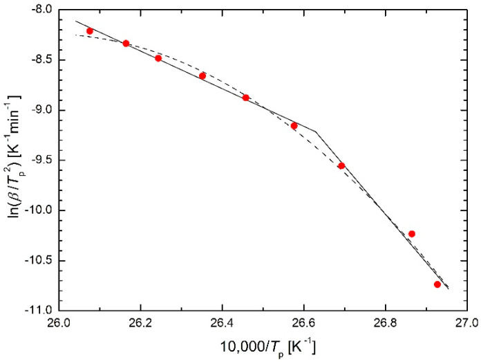
Zhou et al. [5] studied the kinetics of martensitic transformations in Ni-Mn-In-Mg shape memory alloys and obtained a curved Kissinger (Arrhenius) plot. They decided to fit it using two straight lines, see Figure 1 (solid line).
Figure 1.
“Double” Kissinger plot for Ni-Mn-In-Mg shape memory alloy (see [5], Figure 7, solid line) and Kissinger plot based on the analogy of the Equation (5) (dashed line).
This is the simplest approach, giving two very different activation energy values, 156 kJ/mol and 402 kJ/mol. However, it raises more questions than answers:
In terms of materials science: why is the activation energy for heating rates higher than 9.2 K/min 2.5 times lower than for heating rates lower than 9.2 K/min? What is the reason for this step change?
In terms of regression: is it correct to replace an almost smooth arc with two straight lines? If, in a study [5], the heating at heating rates of, e.g., 40 K/min and 35 K/min is not performed and heating at, e.g., 2 K/min and 1 K/min is added, then very likely the straight lines in the Kissinger plot will change their positions substantially, i.e., not only the two values of activation energy will change substantially, but also the value of heating rate separating these straight lines. What is the usefulness of the results obtained in this way?
Deviation from the linear shape of the Arrhenius plot (from “Arrhenius behaviour”) is often referred to as the “non-Arrhenius behaviour” [10] and is distinguished into the “super-Arrhenius behaviour” (concave curve) and “sub-Arrhenius behaviour” (convex curve), e.g., [10,11]. Many authors distinguish only between “concave Arrhenius plot” and “convex Arrhenius plot”, but some of them interchange the terms “concave” and “convex”, e.g., [12]. Many models have been published, especially recently, but almost without exception they are extremely complicated, designed for a very specific scientific problem, without any generality. The aim of this paper is to find a model or relation with similar generality to the original Arrhenius equation.
One of the classical approaches to describing curved Arrhenius plots consisted in a phenomenological description of their shape, mostly using several initial terms of convergent mathematical series in the Arrhenius equation. These were sometimes called “extended Arrhenius equations”, e.g., in [13]. Dozens of papers with extended Arrhenius equations were published especially in the 1970s and 1980s. For example, a logarithmic equation with coefficients A to E (or more) was published by Kanerva et al. [14]:
| (4) |
where the extension consisting in the polynomial of T is supplemented by a ClnT term leading to a multiplicand TC in the original equation. Yang et al. [15] also published a logarithmic equation
| (5) |
where the extension consists of an additional term of the polynomial of 1/T. All of these equations containing three or more parameters usually give a very good fit, but their regression parameters have no physical meaning, i.e., their meaningful interpretation is virtually impossible. An example application of Equation (5) (in fact, its analogy) is given in Figure 1 (dashed line).
Some authors have tried to solve the curvature of the Kissinger plot theoretically. Elder [16,17] suggested adding a term Tm in the Kissinger equation to obtain the so-called generalized Kissinger equation:
| (6) |
where α is the dimensionless degree of reaction or transformation and f(α) is the suitable function that can be described by a suitable dependence on T, R, and E. Parameter m can take the following values [16,17]:
m = 0 leads to the standard Kissinger equation (the Arrhenius assumption is followed [16])
m = 0.5 is predicted by collision theory in the homogeneous gas phase and
m = 1 is predicted by transition state theory.
The author of this paper attempted to use Equation (6) as a regression function in many cases of curved Arrhenius or Kissinger plots, but values of m = 0.5 or m = 1 did not noticeably change the linearity of these plots. Some curvature appeared for values of m in the tens, hundreds, or even thousands, but such values of m have no physical meaning. Formally, Equation (6) corresponds to the Equation (4) in which the first three terms are considered.
Norwisz [18] and, apparently independently, Dutta and Ryan [19] modified the Kissinger equation into the form:
| (7) |
for DSC linear heating with time t:
| (8) |
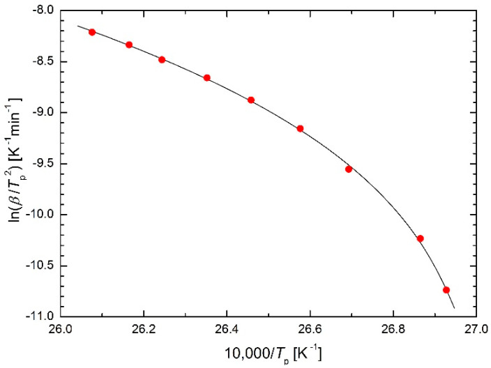
where the initial temperature of heating T0 is taken into account. This modification is indeed able to curve the Arrhenius plot, but it contains one logical weakness: if the heating starts sufficiently low below the temperatures at which the reaction or transformation under study takes place, the initial heating temperature T0 may have hardly any noticeably effect on the kinetics of the process, whereas it plays a crucial role in Equation (7). To clarify the role of T0 in Equation (7), the experimental data from [5] were fitted using Equation (7) as a regression function where T0 is the calculated regression parameter. The successful regression is shown in Figure 2 whereas the calculated value of parameter T0 is quite surprising: T0 = 396 K. Figure 6 in [5] shows that this temperature value T0 cannot be the initial temperature of heating, but it is the temperature at which the heat flux in DSC returns to its constant value after reaching the maximum value, namely for the highest heating rate. In other words, this temperature characterizes the end of the transformation process. From this point of view, Equation (7) can hardly be considered a useful result of theoretical derivation, rather it is a phenomenological equation of the type:
| (9) |
or:
| (10) |
representing only another variant of phenomenological Equations (4) and (5).
Figure 2.
Kissinger plot for Ni-Mn-In-Mg shape memory alloy [5] using Equation (7) as regression function.
A possible explanation for the deviation from the Arrhenius equation is that the reaction does not proceed through a single-step rate-determining mechanism, but proceeds through an intermediate B, e.g., as follows [12]:
| (11) |
Then for the rate constant k of the reaction as a whole, one can write [12,20]:
| (12) |
This equation can be simplified:
| (13) |
The reaction scheme (11) is probably the simplest published scheme used for this reason; a number of more complex schemes can be found in some papers.
Based on Equations (11)–(13), the author of this paper proposed a simpler scheme:
| (14) |
where:
| (15) |
Then the analogy of the Equation (12) can be reconstructed retrospectively:
| (16) |
where the Arrhenius equation can be used for k1 and k2. The resulting regression function then contains the four regression parameters k∞1, k∞2, E1, and E2. However, for better stability of regression calculations, it is better to write the relations for rate constants k1 and k2 in the form:
| (17) |
where T12 is the temperature at which k1 = k2 = k12. For a concave-curved Arrhenius plot (super-Arrhenius behavior) E1 < E2, then k1 < k2 for T < T12 and k1 > k2 for T > T12. Then the resulting regression function contains the four regression parameters k12, T12, E1, and E2.
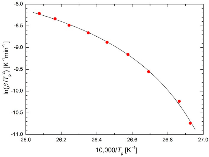
Again, the experimental data from [5] were fitted to validate the presented approach, see Figure 3. As it can be seen, the fitting is successful in this case as well, similar to Figure 2. The regression calculations give a value of temperature T12 = 372 K, which characterizes the position of the curve bending. The calculated activation energies of 143 kJ/mol and 799 kJ/mol can be compared with the values of 156 kJ/mol and 402 kJ/mol [5] obtained by fitting with two straight lines (see also Figure 1): while the E1 values are comparable, the E2 values are in a 2:1 ratio. The sensitivity to adding or removing experimental points at the edges of the test temperature range was also modeled. While the fit with two straight lines is extremely sensitive to such changes, the sensitivity of the fit using regression function (16) is substantially lower, but far from negligible.
Figure 3.
Kissinger plot for Ni-Mn-In-Mg shape memory alloy [5] using Equations (16) and (17) as regression functions.
Formally, the same procedure can be used for a convexly curved Arrhenius plot (sub-Arrhenius behavior), only the regression function (16) must be replaced by k = k1 + k2.
2. Derivation of the Modified Arrhenius Equation
The linearization plot is used not only in the case of the Arrhenius equation. The cumulative distribution function (cdf) of the Weibull distribution used in survival analysis, reliability engineering, failure analysis, etc., is as follows:
| (18) |
where a is the scale parameter and b is the shape parameter. This cdf can be linearized:
| (19) |
that is, the term on the left side of this equation is a linear function of ln x. The plot with axes:
| (20) |
where is empirical cdf, is called the Weibull plot. If in a concave-curved Weibull plot, its left-end points to the lnx0 on the x-axis, it is an unmistakable indication that the three-parameter Weibull distribution:
| (21) |
should be used, i.e., formally x is replaced by x − x0. By analogy, if in a concave-curved Arrhenius plot its right end tends towards the 1/T0 on 1/T-axis, the replacement of the temperature T by the temperature difference T − T0 should be considered in the Arrhenius equation:
| (22) |
For a three-parameter Weibull distribution, the relation x > x0 must be held. According to Equation (22), k = 0 for T→T0 but for many reasons it should be zero even for T < T0. Then Equation (22) must be replaced by the more accurate equation:
| (23) |
Before discussing the newly derived regression function (23), let it be used for fitting the experimental data from [5], see Figure 4. It can be seen that the regression is again very successful. The regression calculations give T0 = 363 K. Figure 6 in [5] shows that at this temperature the heat flux in DSC starts to increase from its constant values at all heating rates. This means that this temperature is the initial temperature of the described transformation, in this case austenitization. Thus, only one parameter with a well-defined physical meaning has been added to the original Arrhenius equation (in the previous case they were two parameters), which causes the required curvature of the Arrhenius plot. This achieved the desired goal of this paper. It now remains to verify the suitability of the regression function (23) in the widest possible range of scientific research. Therefore, some specific cases will be presented.
Figure 4.
Kissinger plot for Ni-Mn-In-Mg shape memory alloy [5] using the modified Arrhenius Equation (23) as regression function.
Formally, for convexly curved Arrhenius plot (sub-Arrhenius behavior) the regression function:
| (24) |
can be applied (some of the first attempts look very promising). However, the physical interpretation of temperature T0 is likely to be a very difficult problem in this case.
3. Verification of the Suitability of the Modified Arrhenius Equation
3.1. Materials Science
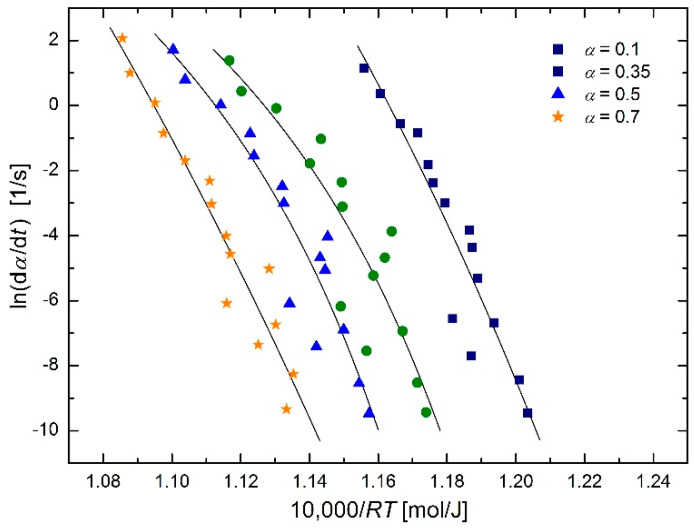
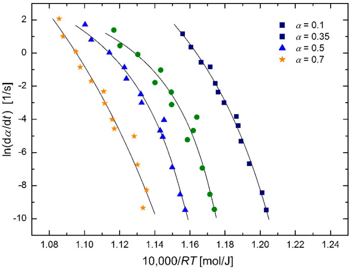
The austenitization kinetics of SA 508 Gr.3 steel was studied by Luo et al. [2] using an isoconversional method. They described the dependence of the phase transformation rate on temperature using the Arrhenius equation (see Figure 5 in [2]):
| (25) |
where α is the extent of conversion. The authors replaced the product Af (α) by a new pre-exponential factor B(α) and took into account the dependence of effective activation energy on the extent of conversion E(α):
| (26) |
Results of regression using the modified regression function:
| (27) |
are shown in Figure 5; the temperature T0 values (means and standard deviations) for different extents of conversion α are given in Table 1.
Figure 5.
Arrhenius plot for austenitization of SA 508 Gr.3 steel using isoconversional method [2] based on the modified Arrhenius equation in the form of Equation (27).
Table 1.
T0 temperatures for different conversions corresponding to the plots in Figure 5.
| Conversion α | 0.1 | 0.35 | 0.5 | 0.7 | Mean ± s.d. |
|---|---|---|---|---|---|
| temperature T0 [K] | 801 | 943 | 959 | 753 | 864 ± 51 |
| temperature T0 [°C] | 528 | 670 | 686 | 480 | 591 ± 51 |
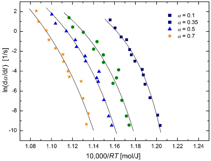
Plots in Figure 5 show certain curvatures. However, a closer look at the figure reveals that every third and fifth lowest experimental point for all conversions appear to be outliers. Without performing any statistical test for outliers, these eight points (i.e., the points with y-values ≈ −6.3 and ≈ −7.5) were removed and the previous regression calculations were repeated. The results are shown in Figure 6 and Table 2.
Figure 6.
Arrhenius plot for austenitization of SA 508 Gr.3 steel using isoconversional method [2] (reduced data) based on the modified Arrhenius equation in the form of Equation (27).
Table 2.
T0 temperatures for different conversions corresponding to the plots in Figure 6 (reduced data).
| Conversion α | 0.1 | 0.35 | 0.5 | 0.7 | Mean ± s.d. |
|---|---|---|---|---|---|
| temperature T0 [K] | 904 | 997 | 1005 | 938 | 971 ± 17 |
| temperature T0 [°C] | 671 | 724 | 732 | 665 | 698 ± 17 |
It can be seen that the T0 values in Table 2 are higher and closer together than the values in Table 1. Therefore, another regression of the reduced data set was performed, this time with a regression parameter T0 common to all four conversion values 0.1, 0.35, 0.5 and 0.7. This resulted in T0 = 966.8 K with an estimated standard deviation of 9.1 K, i.e., T0 = (967 ± 9) K = (694 ± 9) C. Graphical output of these calculations is shown in Figure 7.
Figure 7.
Arrhenius plot for austenitization of SA 508 Gr.3 steel using isoconversional method [2] (reduced data) based on the modified Arrhenius equation in the form of Equation (27), with common regression parameter T0 for all α values.
Austenitization starts at temperature Ac1, which seems to be close to the obtained value of temperature T0. The temperatures Ac1 are not usually published, but they can be calculated from their chemical composition, which for SA 508 Gr.3 steel is given in Table 3.
Table 3.
Chemical composition of SA508 Gr.3 steel [2].
| Element | C | Mn | Si | Ni | Cr | Mo | V | Al | N | Fe |
|---|---|---|---|---|---|---|---|---|---|---|
| composition wt.% | 0.20 | 1.47 | 0.17 | 0.89 | 0.13 | 0.51 | 0.001 | 0.039 | 0.014 | bal. |
For the calculation of the Ac1 temperature, the paper [21] was chosen, which is sufficiently new and takes into account as many elements from Table 3 as possible. It provides the equation:
| (28) |
where the symbols of chemical elements are to be replaced by their content in weight percent. Equation (28) for values gives Ac1 = 696.7 °C, with a recommended standard deviation of 9.2 °C [21], then the result can be written as Ac1 = (697 ± 9) °C = (970 ± 9) K. The agreement with the temperature T0 (see mean value in Table 2 and value T0 = (967 ± 9) K = (694 ± 9) °C obtained in common regression) is practically perfect. It can then be argued that the temperature T0 from the modified Arrhenius equation is directly Ac1 temperature of studied steel (logical judgment is supplemented by numerical verification).
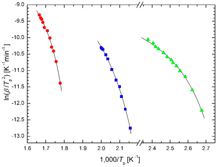
DSC studies on the transformation kinetics of Ga7.5Se92.5 chalcogenide glass [22] (one crystallization peak) and of Si12.5Te87.5 chalcogenide glass [23] (two separated crystallization peaks) applying the isoconversional method were performed by El-Oyoun. The results are plotted in the Kissinger plots in Figure 8. The values of T0 are 339 K for Ga7.5Se92.5 chalcogenide glass, 413 K for the first crystallization peak and 522 K for the second crystallization peak, both for Si12.5Te87.5 chalcogenide glass. Comparing these temperatures with corresponding DSC curves [22,23], the T0 values characterize approximately the onset of heat flux for the lowest heating rates.
Figure 8.
Kissinger plot for crystallization of Ga7.5Se92.5 chalcogenide glass [22] (triangles) and of Si12.5Te87.5 chalcogenide glass [23] (two separated crystallization peaks, squares and circles) based on the modified Arrhenius Equation (23).
3.2. Food Storage
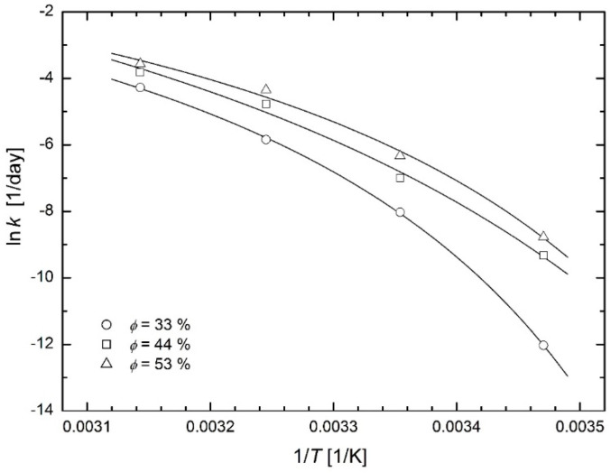
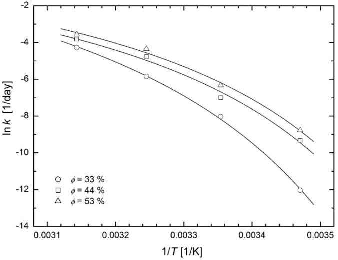
Sá and Sereno [24] studied the browning kinetics of onion and strawberry during the storage at temperatures 5, 15, 25, 35 and 45 °C and at relative humidity 33, 44 and 53 %. The extent of browning of the freeze-dried Portuguese red onion (Allium cepa L.) was determined by the measurement of the absorbance of the filtered extract in 1 cm quartz cells at wavelength of 420 nm using a UV/Vis Lambda 2 Spectrophotometer (Perkin Elmer, Connecticut, USA), see the official ADOGA method [25]. The authors could then determine the corrected reaction rate constants and plot them in the Arrhenius plot (see Figure 3 in [24]) with the Arrhenius straight lines and the curves corresponding to the Williams-Lander-Ferry model (WLF model) [26]. Figure 9 and Figure 10 in this paper show that the modified Arrhenius plot based on Equation (23) leads to a successful fit of the considered experimental data. Figure 9 shows fit with individual values of temperature T0 for each relative humidity: 261 K for 33%, 242 K for 44% and 255 K for 53%. Figure 10 shows the fits with the common value of temperature T0 = 256 K = −18 °C for all relative humidity values. Temperatures below −18 °C are used as a standard for long-term storage of food. The WLF model used by Sá and Sereno [24] to fit experimental data leads to the same fitting curves, as will be discussed in the Discussion chapter.
Figure 9.
Modified Arrhenius plots for reaction rate constants of browning in freeze-dried onion at various relative humidity [24] (individual values of temperature T0 for each relative humidity).
Figure 10.
Modified Arrhenius plots for reaction rate constants of browning in freeze-dried onion at various relative humidity [24] (common value of temperature T0 = −18 °C for all values of relative humidity).
3.3. Botany
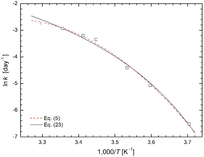
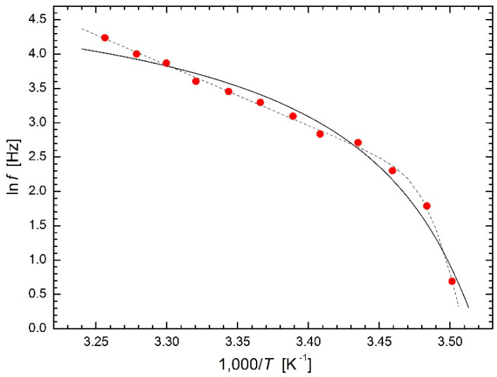
Curved Arrhenius plots in the studies of biological processes (especially in the context of plants) were discussed by Wolfe and Bagnall [27] as early as 1980. In 44 references many models of various complexity explaining the curvature of the Arrhenius plots are given. Additionally, Nishiyama et al. [3] studied the temperature dependence of the respiration rate of camellia leaves (Camellia japonica) and obtained the curved Arrhenius plot. They compared the fitting using Equation (5) (see dashed line in Figure 11) with the split into two straight lines (it was experimental data of Nishiyama et al in [3] that were the basis for the paper of Yang et al. [15]). However, even in this case the modified Arrhenius Equation (23) gives a reasonably good fit, only slightly worse than Equation (5), see solid line in Figure 11. While Equation (5) is completely phenomenological and contains parameters without any physical meaning, the value of temperature T0 = 235 K = −38 °C obtained from the regression calculations using Equation (23) as regression function apparently represents the temperature below which respiratory processes no longer occur.
Figure 11.
Modified Arrhenius plot for respiration rate of camellia leaves [3] based on Equation (23) is compared with the fit based on Equation (5).
3.4. Microbiology
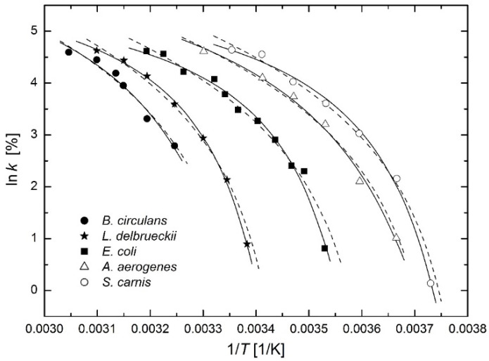
Ratkowski et al. [28] drew the Arrhenius plots of the growth rates of bacterial cultures reported by Johnson et al. [29] (see p. 199). The growth rates of the studied bacterial cultures reach their maxima at certain temperatures. Johnson et al. [29] considered relative growth rates (maximum of growth rate = 100 %) and Ratkowski et al. [28] focused only on the temperature range where growth rates decrease with decreasing temperature (i.e., with increasing 1/T). They used fully phenomenological regression function:
| (29) |
proposed by Ohta and Hirahara [30]. In Figure 12 the Arrhenius plots of relative growth rates are drawn with fits based on the modified Arrhenius Equation (23) (solid lines) and on phenomenological regression function (29) (dashed lines). The modified Arrhenius Equation (23) leads to a better fit, especially for the highest growth rates. On the other hand, with regard to the number of regression parameters (only two) and the time of publication (1977), the function (29) represented a significant advance in the phenomenological description of growth of bacterial cultures at that time.
Figure 12.
Arrhenius plots for the relative growth rates of bacterial cultures [28,29] based on the modified Arrhenius Equation (23) (solid lines) and on phenomenological regression function (29) (dashed lines). See Table 4 for full names of bacterial cultures.
The values of temperature T0 obtained from regression calculations are shown in Table 4 for both regression functions (23) and (29). Additionally, the values published by Ratkowski et al. [28] are added for comparison. The negligible differences between the second to last column and the last column may be due to different regressions: y = lnk in this paper and y = in paper [28]. Finally, it can be said that temperature T0 (in both Equations (23) and (29)) can be interpreted as the temperature below which the bacterial culture under consideration does not grow.
Table 4.
Temperatures T0 for different bacterial cultures corresponding to the plots in Figure 12.
| No | Bacterial Culture | T0 [K] (23) | T0 [°C] (23) | T0 [K] (29) | T0 [K] [28] |
|---|---|---|---|---|---|
| 1 | Bacillus circulans | 283.4 | 10.3 | 296.0 | 296 |
| 2 | Lactobacillus delbrueckii | 283.6 | 10.5 | 290.9 | 290 |
| 3 | Escherichia coli | 271.3 | −1.8 | 277.8 | 276 |
| 4 | Aerobacter aerogenes | 254.1 | −19.0 | 267.4 | 267 |
| 5 | Sporotrichum carnis | 257.3 | −15.9 | 264.7 | 264 |
3.5. Zoology
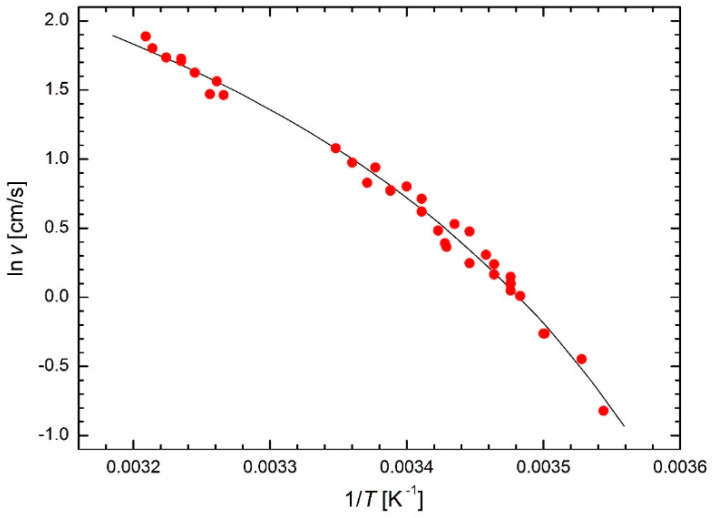
Laidler [4] summarized some unusual applications of the Arrhenius law in the animal kingdom, e.g., in entomology (chirping of tree crickets, creeping of ants or flashing of fireflies). In particular, the creeping of the ant Liometopum apiculatum (described by G. Mayr in 1870, widespread in southwestern United States and from northwestern to southeastern Mexico) using the Arrhenius law was studied by Crozier [31] who used the results of measurements of ant speed versus temperature made by Shapley [32]. The Arrhenius plot of ant speed values (excluding the two outliers specified by Shapley and the third outlier removed by Crozier) is shown in Figure 13. The fit based on the modified Arrhenius Equation (23) leads to temperature T0 = 252 K = −21 °C. It can be interpreted as the temperature at which the movement of the ants under study stops.
Figure 13.
Modified Arrhenius plots for the speed of ant Liometopum apiculatum [31,32] based on Equation (23).
Laidler [4] also presented the measurement of the frequency of terrapin’s heartbeat at different temperatures made by Martin [33]. The Arrhenius plot of the rate of terrapin’s heartbeat is shown in Figure 14. The experimental data are fitted excellently using Equations (16) and (17) as regression function, where temperature T12 = 285 K = 12 °C separates two nearly linear parts of the plot with different slopes, i.e., with different values of activation energy. A considerably worse fit is obtained using the modified Arrhenius Equation (23) but, on the other hand, regression parameter T0 = 277 K = 4 °C represents the limit temperature below which terrapin’s heartbeat appears to stop.
Figure 14.
Modified Arrhenius plots for the rate of terrapin’s heartbeat [4,31] based on Equation (23) (solid line) compared with the fit using Equations (16) and (17) as regression function (dashed line).
4. Discussion
The effort to cope with the curvature of the Arrhenius plot is very old and many phenomenological equations have been published, e.g., Equations (4)–(7), (9) and (10). Some of them have been published and used only a few times but, e.g., the supplement of C/(RT)2 as an addend in Equation (5) (or exp[C/(RT)2] as a multiplicand before logarithmization) causing curvature of the Arrhenius plot) has been used very often as a so-called Bässler-like factor [3,34]. Unfortunately, parameter C has no physical meaning and after adding the Bässler factor in Equation (5), parameter B loses its previous physical meaning: B = −E (activation energy).
According to the Arrhenius Equation (1), the reaction rates at very low temperatures are very small but non-zero. This is acceptable for chemical reactions of simple chemicals. On the other hand, many processes whose temperature dependence is also described by the Arrhenius equation, can proceed only above a certain temperature but they cannot proceed below it. In materials science, polymorphous materials can exist in a particular form or crystal structure only above certain temperatures (often within a certain temperature range), e.g., austenite (in equilibrium state) can exist only above the temperature Ac1. Additionally, plant and animal life can exist above certain individual temperatures. The modified Arrhenius Equation (23) respects these facts: k > 0 only for T > T0, for T < T0 is k = 0.
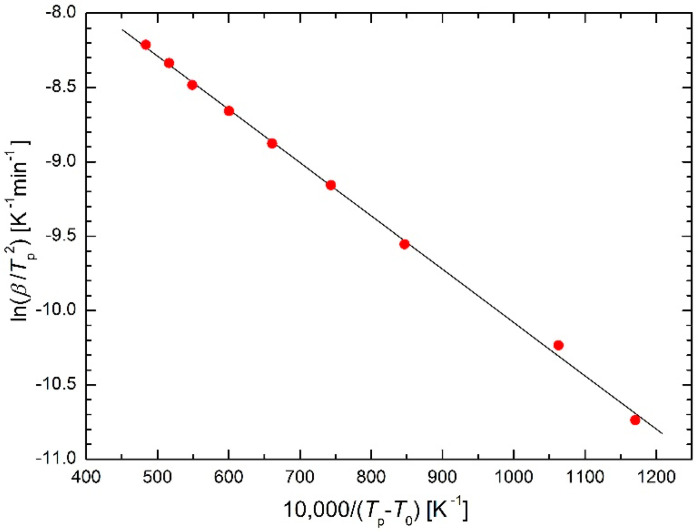
The validity of the modified Arrhenius Equation (23) can be illustrated by drawing in the plot lnk vs. 1/(T − T0) instead of in the usual plot lnk vs. 1/T where the linear course is obtained with the slope −Em/R. This is shown in Figure 4 redrawn in the plot lnk vs. 1/(T − T0), see Figure 15. A similar procedure is used in the Weibull plot when a three-parameter Weibull distribution is considered: ln x-axis is replaced by ln(x − −x0) axis, see Equation (20).
Figure 15.
Kissinger plot for Ni-Mn-In-Mg shape memory alloy [5] using the modified Arrhenius Equation (23) as regression function. Replacing 1/T axis by 1/(T − T0), a linear plot is obtained instead of a curved plot.
One of the criteria for the suitability of the regression function is the sum of the squares of the deviations between the measured and calculated values of the observed quantity. These sums are compared in Table 5 for the Kissinger plot for Ni-Mn-In-Mg shape memory alloy [5], see Figures 1 to 4. It can be seen that the worst results are obtained for the twice (“per partes”) used linear dependence and phenomenological function analogous to Equation (5). The lowest sum is obtained for Equation (7) whose derivation is rather problematic, see Introduction chapter. Comparable values of the sum are obtained for the two newly presented functions described by Equation (16) (supplemented by Equation (17)) and Equation (23).
Table 5.
Comparison of sums of squares in the Kissinger plot for Ni-Mn-In-Mg shape memory alloy [5] using the presented equations as regression functions.
| Equation(s) | Figure | S |
|---|---|---|
| (1) (twice) | 1 | 0.026706 |
| analogy of (5) | 1 | 0.031670 |
| (7) | 2 | 0.003730 |
| (16) and (17) | 3 | 0.009765 |
| (23) | 4 | 0.008962 |
Although the symbol E denotes the (activation) energy in the original Arrhenius Equation (1), as well as in the modified Arrhenius Equation (23), the two energies differ significantly. Let the energy in Equation (1) henceforth be denoted as EA and in Equation (23) as Em. The activation energy EA is usually defined as:
| (30) |
therefore, the slope of the Arrhenius plot is equal to −EA/R, see also Equation (2). Differentiation (30) of the modified Arrhenius Equation (23) gives:
| (31) |
Two limits can be easily determined:
| (32) |
as well as three equalities:
| (33) |
Equation (32) shows that the slope of the modified Arrhenius plot for higher temperatures is approximately equal to the slope of the classical Arrhenius plot but approaching T0 it grows above all limits. Equation (33) implies that Em can be orders of magnitude lower than EA. On the other hand, Em is really constant (independent of temperature), while EA is dependent on temperature in the curved Arrhenius plot (as invariable constant is only for the classical Arrhenius Equation (1)). For example, for kinetic Equation (4) the differentiation (30) gives the value:
| (34) |
and for Equation (5):
| (35) |
It is the constant (activation) energy Em and the single parameter T0 (the lowest temperature at which the process under study still takes place), which controls the curvature of the curved Arrhenius plot, which are the main advantages of the newly presented modified Arrhenius Equation (23) compared to a number of other more or less phenomenological relations containing one or often more parameters without any physical meaning.
After deriving and verifying the suitability of the modified Arrhenius Equation (23), the author of this paper tried to find some similar equations, i.e., equations containing the exp[B/(T − T0)] term or the B/(T − T0) term after logarithmization. They have been found in fields of science far from the fields mentioned above:
- The Vogel−Fulcher−Tammann equation (VFT equation) [35,36,37] is used to describe the viscosity of liquids as a function of temperature, especially near the glass transition:
where η0, B, and TVF (typically lying about 50 °C below the glass transition temperature) are empirical material-dependent parameters. García-Colín et al. [38] have not very convincingly attempted to build this purely empirical equation on a theoretical basis.(36) - In the study of shear creep and recovery of elastomers, Conant et al. [39] published an empirical equation for temperature dependence of creep or recovery time tc:
where Cα, Cβ, and b are empirical constants. They mentioned the similarity of Equation (36) to the Arrhenius equation and called constant b as “correction” term.(37) - When studying dielectric relaxation in some simple alcohols, Davidson and Cole [40] found that the temperature dependence of relaxation times deviates systematically from the Arrhenius law. Most of their data could be fitted to the expression:
For glycerol and n-propanol, these authors even found that the temperature values T∞ determined from electric relaxation times agree with the temperature values TVF (see VFT equation) found in the viscosity studies performed by Tammann and Hesse [37]. This agreement T∞ = TVF means that there are no different specific temperatures for the individual physical quantities, but only one common temperature characterizing the material under study as such.(38)
This means that for the three reciprocal values 1/η, 1/tc and 1/τc, the modified Arrhenius Equation (23) holds. A broader presentation of the interconnection of the Kissinger method used in the study of kinetic processes in materials with many phenomena in other fields of science was made by Vyazovkin in his excellent review [41].
The authors of the Williams-Lander-Ferry model [26] came out of the VFT equation [35,37]. The opposite path is very simple to show. If the reference temperature is identified with glass transition temperature Tg, the VFT equation can be written in the form:
| (39) |
where η is viscosity and ρ is the density of the studied liquid. Since the product ρT is not very temperature sensitive (especially not compared to the right side of the equation), the simplified left side of the equation ln(η/ηg) can be considered. Then Equation (38) can be rewritten into the form:
| (40) |
After the substitutions:
| (41) |
logarithmized VFT Equation (36) is obtained.
Soesanto and Williams [42] prefer the WLF equation to the VFT equation (and all other equations of this type, i.e., (36), (37), including the modified Arrhenius Equation (23)). They argue for clarified meaning of the parameters of the WLF equation Tg, ηg, c1, and c2. The meaning of the parameters Tg and ηg is unquestionable, but parameters c1 and c2 are only phenomenological parameters without any physical meaning. In contrast, the parameters in Equation (23) have in principle a clear physical meaning: the meaning of k∞ is the same as in the original Arrhenius equation, E represents some analogy of activation energy (independent of temperature) and T0 is the temperature characterizing the material under study, common to more physical properties of this material. Moreover, the parameters k∞, E, and T0 are independent of each other, while the parameters of the WLF equation Tg, ηg, c1, and c2 are not (cannot be) independent. This means that for regression, one parameter (usually Tg) must be predetermined and only the remaining three parameters can be calculated in the regression procedure.
As shown above, the regression function (16) accompanied by Equation (17), as well as the modified Arrhenius Equation (23) allow a successful regression of concave Arrhenius plots. On the other hand, their abilities to describe complex chemical reactions are limited. This limitation is quite fundamental and consists of a small number of regression parameters − in principle, it is not possible to accurately describe multi-step reactions using only three or four parameters. Probably the simplest published reaction (11) used in this case had to be further simplified to the reaction with the scheme (14), in fact with the scheme:
| (42) |
in order to limit the number of regression parameters in the regression function (16) accompanied by Equation (17) to four. The modified Arrhenius Equation (23) contains only three regression parameters and also cannot be used successfully in the case of more complex phenomena, such as relaxation processes in gas-containing plasmas [43,44]. Overleaf, the dielectric relaxation in some simple alcohols studied by Davidson and Cole [40] has been successfully described using Equation (38), which is actually another form of the modified Arrhenius Equation (23).
5. Conclusions
The presented findings can be summarized as follows:
In the case where the experimental Arrhenius plot consists of two approximately linear parts, the fit using regression function (16) accompanied by Equation (17) gives a successful result. The use of the regression function (16) is much more suitable than using two independent straight lines.
For the generally curved Arrhenius plot, the regression function (23) is very suitable. Only one parameter, T0 with clear physical meaning (the lowest temperature at which the studied process is still running) controls the curvature of the Arrhenius plot. For T0→0 the modified Arrhenius Equation (23) transitions smoothly into the original Arrhenius Equation (1).
The two models presented for a concave-curved Arrhenius plot (super-Arrhenius behavior) can be simply modified for the convex-curved Arrhenius plot (sub-Arrhenius behavior).
In addition to chemistry, the newly proposed model (23) can also be used in materials science, food storage, botany, microbiology and even in zoology, as has been demonstrated.
In the past, phenomenological equations corresponding to the modified Arrhenius Equation (23) have been used for the temperature dependence description of liquid viscosity, creep or recovery time and dielectric relaxation time. Its validity seems to be very broad in many different fields of science and technology. However, it is necessary to try to interpret the meaning of temperature T0, as it has been identified with the temperature Ac1 in the austenitization of SA 508 Gr.3 steel.
Also, the WLF equation is essentially equivalent to the modified Arrhenius Equation (23). However, its parameters Tg, ηg, c1, and c2 are not independent and for regression one parameter (usually Tg) must be specified in advance and only the remaining three parameters can be calculated in regression procedure.
When the temperature dependence of several properties of a single material is studied using the modified Arrhenius Equation (23), the obtained temperature values T0 represent the only one common temperature characterizing this material as a whole, not its individual properties.
Acknowledgments
Financial support from the Ministry of Defence of the Czech Republic within the Organization Development Project is gratefully acknowledged. In addition, the author is grateful to all authors whose original experimental results were used for regression calculations presented in this paper.
Funding
The research received no external funding.
Institutional Review Board Statement
Not applicable.
Data Availability Statement
Data sharing is not applicable to this article.
Conflicts of Interest
The author declares no conflict of interest.
Sample Availability
Samples of the compounds are not available from the author.
Footnotes
Publisher’s Note: MDPI stays neutral with regard to jurisdictional claims in published maps and institutional affiliations.
References
- 1.Arrhenius S. Über die Reaktionsgeschwindigkeit bei der Inversion von Rohrzucker durch Säuren. Z. Physik. Chem. 1889;4:226–248. doi: 10.1515/zpch-1889-0416. [DOI] [Google Scholar]
- 2.Luo X., Han L., Gu J. Study on Austenitization Kinetics of SA508 Gr.3 Steel Based on Isoconversional Method. Metals. 2016;6:8. doi: 10.3390/met6010008. [DOI] [Google Scholar]
- 3.Nishiyama M., Kleijn S., Aquilanti V., Toshio Kasai T. Temperature dependence of respiration rates of leaves, 18O-experiments and super-Arrhenius kinetics. Chem. Phys. Lett. 2009;482:325–329. doi: 10.1016/j.cplett.2009.10.005. [DOI] [Google Scholar]
- 4.Laidler K.J. Unconventional Applications of the Arrhenius Law. J. Chem. Educ. 1972;49:343–344. doi: 10.1021/ed049p343. [DOI] [Google Scholar]
- 5.Zhou Z.N., Yang L., Li R.C., Li J., Hu Q.D., Li J.G. Martensitic transformations and kinetics in Ni-Mn-In-Mg shape memory alloys. Intermetallics. 2018;92:49–54. doi: 10.1016/j.intermet.2017.09.016. [DOI] [Google Scholar]
- 6.Kissinger H.E. Reaction Kinetics in Differential Thermal Analysis. Anal. Chem. 1957;29:1702–1706. doi: 10.1021/ac60131a045. [DOI] [Google Scholar]
- 7.Blaine R.L., Kissinger H.E. Homer Kissinger and the Kissinger equation. Thermochim. Acta. 2012;540:1–6. doi: 10.1016/j.tca.2012.04.008. [DOI] [Google Scholar]
- 8.Holba P., Šesták J. Imperfections of Kissinger Evaluation Method and Crystallization Kinetics. Glass Phys. Chem. 2014;40:486–495. doi: 10.1134/S1087659614050058. [DOI] [Google Scholar]
- 9.Šesták J., Holba P., Živković Ž. Doubts on Kissinger´s method of kinetic evaluation based on several conceptual models showing the difference between the maximum of reaction rate and the extreme of a DTA peak. J. Min. Metall. Sect. B-Metall. 2014;50:77–81. doi: 10.2298/JMMB130902006S. [DOI] [Google Scholar]
- 10.Rosa A.C.P., Jr., Cruz C., Santana W.S., Moret M.A. Characterization of the non-Arrhenius behavior of supercooled liquids by modeling nonadditive stochastic systems. Phys. Rev. E. 2019;100:022139. doi: 10.1103/PhysRevE.100.022139. [DOI] [PubMed] [Google Scholar]
- 11.Coutinho N.D., Silva V.H.C., Mundim K.C., de Oliveira H.C.B. Description of the effect of temperature on food systems using the deformed Arrhenius rate law: Deviations from linearity in logarithmic plots vs. inverse temperature. Rend. Lincei. 2015;26:141–149. doi: 10.1007/s12210-015-0407-4. [DOI] [Google Scholar]
- 12.Truhlar G.M., Kohen A. Convex Arrhenius plots and their interpretation. Proc. Natl Acad. Sci. USA. 2001;98:848–851. doi: 10.1073/pnas.98.3.848. [DOI] [PMC free article] [PubMed] [Google Scholar]
- 13.Adams P.A., Sheppard J.G., Ridler G.M., Ridler P.F. New Three-parameter Empirical Extension of the Arrhenius Equation suitable for the Precise Evaluation of Pseudothermodynamic Activation Parameters in Chemical Kinetics. J. Chem. Soc. Faraday Trans. 1. 1978;74:1500–1506. doi: 10.1039/f19787401500. [DOI] [Google Scholar]
- 14.Kanerva L.T., Euranto E.K., Cleve N.J. On the Accuracy and Significance in Determination of the Temperature Dependence of Activation Energy in Neutral Ester Hydrolysis and Solvolytic Substitution Reaction. Acta Chem. Scand. B. 1983;37:85–92. doi: 10.3891/acta.chem.scand.37b-0085. [DOI] [Google Scholar]
- 15.Yang H.C., Ge Y.C., Su K.H., Chang C.C., Lin K.C., Aquilanti V., Kasai T. Temperature effect on water dynamics in tetramer phosphofructokinase matrix and the super-Arrhenius respiration rate. Sci. Rep. 2021;11:383. doi: 10.1038/s41598-020-79271-5. [DOI] [PMC free article] [PubMed] [Google Scholar]
- 16.Elder J.P. Integral-Differential Relationships in Thermal Analysis. In: Johnson J.F., Gill P.S., editors. Analytical Calorimetry. Volume 5. Plenum Press; New York, NY, USA: 1984. pp. 255–264. [Google Scholar]
- 17.Elder J.P. The General Applicability of the Kissinger Equation in Thermal Analysis. J. Therm. Anal. 1985;30:657–669. doi: 10.1007/BF01913612. [DOI] [Google Scholar]
- 18.Norwisz J. The kinetic equation under linear temperature increase conditions. Thermochim. Acta. 1978;25:123–125. doi: 10.1016/0040-6031(78)80048-3. [DOI] [Google Scholar]
- 19.Dutta A., Ryan M.E. The relationship between isothermal and non-isothermal kinetics for thermoset characterization. Thermochim. Acta. 1979;33:87–92. doi: 10.1016/0040-6031(79)87031-8. [DOI] [Google Scholar]
- 20.Albery W.J., Robinson B.H. Measurement of Enthalpies and Heat Capacities of Activation by Differential Methods. Trans. Faraday Soc. 1969;65:980–991. doi: 10.1039/tf9696500980. [DOI] [Google Scholar]
- 21.Trzaska J. Calculation of Critical Temperatures by Empirical Formulae. Arch. Metall. Mater. 2016;61:981–986. doi: 10.1515/amm-2016-0167. [DOI] [Google Scholar]
- 22.El-Oyoun M.A. Evaluation of the transformation kinetics of Ga7.5Se92.5 chalcogenide glass using the theoretical method developed and isoconversional analyses. J. Alloys Compd. 2010;507:6–15. doi: 10.1016/j.jallcom.2010.07.166. [DOI] [Google Scholar]
- 23.El-Oyoun M.A. DSC studies on the transformation kinetics of two separated crystallization peaks of Si12.5Te87.5 chalcogenide glass: An application of the theoretical method developed and isoconversional method. Mater. Chem. Phys. 2011;131:495–506. doi: 10.1016/j.matchemphys.2011.10.009. [DOI] [Google Scholar]
- 24.Sá M.M., Sereno A.M. The kinetics of browning measured during the storage of onion and strawberry. Int. J. Food Sci. Technol. 1999;34:343–349. doi: 10.1046/j.1365-2621.1999.00276.x. [DOI] [Google Scholar]
- 25.Association for Dehydrated Onion and Garlic Products . Official Standards and Methods of the American Dehydrated Onion and Garlic Association for Dehydrated Onion and Garlic Products. ADOGA; San Francisco, CA, USA: 1976. [Google Scholar]
- 26.Williams M.L., Landel R.F., Ferry J.D. The temperature dependence of relaxation mechanisms in amorphous polymers and other glass forming liquids. J. Am. Chem. Soc. 1955;77:3701–3707. doi: 10.1021/ja01619a008. [DOI] [Google Scholar]
- 27.Wolfe J., Bagnall D.J. Arrhenius Plots—Curves or Straight Lines? Ann. Bot. 1980;45:485–488. doi: 10.1093/oxfordjournals.aob.a085848. [DOI] [Google Scholar]
- 28.Ratkowsky D.A., Olley J., McMeekin T.A., Ball A. Relationship Between Temperature and Growth Rate of Bacterial Cultures. J. Bacteriol. 1982;149:1–5. doi: 10.1128/jb.149.1.1-5.1982. [DOI] [PMC free article] [PubMed] [Google Scholar]
- 29.Johnson F.H., Eyring H., Stove B.J. The theory of Rate Processes in Biology and Medicine. Wiley; New York, NY, USA: 1974. p. 703. [Google Scholar]
- 30.Ohta F., Hirahara T. Rate of Degradation of Nucleotides in Cooling-stored Carp Muscle. Mem. Fac. Fish. Kagoshima Univ. 1977;26:97–102. [Google Scholar]
- 31.Crozier W.J. On the critical thermal increment for the locomotion of a diplopod. J. Gen. Physiol. 1924;7:123–136. doi: 10.1085/jgp.7.1.123. [DOI] [PMC free article] [PubMed] [Google Scholar]
- 32.Shapley H. Thermokinetics of Liometopum apiculatum Mayr. Proc. Natl. Acad. Sci. USA. 1920;6:204–211. doi: 10.1073/pnas.6.4.204. [DOI] [PMC free article] [PubMed] [Google Scholar]
- 33.Martin E.G. The inhibitory influence of potassium chloride on the heart, and the effect of variations of temperature upon this inhibition and upon vagus inhibition. Am. J. Physiol. 1904;11:370–393. doi: 10.1152/ajplegacy.1904.11.4.370. [DOI] [Google Scholar]
- 34.Bässler H. Viscous flow in supercooled liquids analyzed in terms of transport theory for random media with energetic disorder. Phys. Rev. Lett. 1987;58:767–770. doi: 10.1103/PhysRevLett.58.767. [DOI] [PubMed] [Google Scholar]
- 35.Vogel D.H. Das Temperaturabhaengigkeitsgesetz der Viskositaet von Fluessigkeiten. Phys. Z. 1921;22:645–646. [Google Scholar]
- 36.Fulcher G.S. Analysis of recent measurements of the viscosity of glasses. J. Am. Ceram. Soc. 1925;8:339–355. doi: 10.1111/j.1151-2916.1925.tb16731.x. [DOI] [Google Scholar]
- 37.Tammann G., Hesse W. Die Abhängigkeit der Viscosität von der Temperatur bie unterkühlten Flüssigkeiten. Z. Anorg. Allg. Chem. 1926;156:245–257. doi: 10.1002/zaac.19261560121. [DOI] [Google Scholar]
- 38.García Colin L.S., del Castillo L.F., Goldstein P. Theoretical basis for the Vogel–Fulcher–Tammann equation. Phys. Rev. B. 1989;40:7040–7044. doi: 10.1103/PhysRevB.40.7040. [DOI] [PubMed] [Google Scholar]
- 39.Conant F.S., Hall G.L., Lyons W.J. Equivalent Effects of Time and Temperature in the Shear Creep and Recovery of Elastomers. J. Appl. Phys. 1950;21:499–504. doi: 10.1063/1.1699693. [DOI] [Google Scholar]
- 40.Davidson D.W., Cole R.H. Dielectric Relaxation in Glycerol, Propylene Glycol, and n-Propanol. J. Chem. Phys. 1951;19:1484–1490. doi: 10.1063/1.1748105. [DOI] [Google Scholar]
- 41.Vyazovkin S. Kissinger Method in Kinetics of Materials: Things to Beware and Be Aware of. Molecules. 2020;25:2813. doi: 10.3390/molecules25122813. [DOI] [PMC free article] [PubMed] [Google Scholar]
- 42.Soesanto T., Williams M.C. Interpretation of Viscosity for Concentrated and Dilute Sugar Solutions. J. Phys. Chem. 1981;85:3338–3341. doi: 10.1021/j150622a026. [DOI] [Google Scholar]
- 43.Laporta V., Heritier K.L., Panesi M. Electron-vibration relaxation in oxygen plasmas. Chem. Phys. 2016;472:44–49. doi: 10.1016/j.chemphys.2016.03.002. [DOI] [Google Scholar]
- 44.Laporta V., Bruno D. Electron-vibration energy exchange models in nitrogen-containing plasma flows. J. Chem. Phys. 2013;138:104319. doi: 10.1063/1.4794690. [DOI] [PubMed] [Google Scholar]
Associated Data
This section collects any data citations, data availability statements, or supplementary materials included in this article.
Data Availability Statement
Data sharing is not applicable to this article.


