Multi-scanner Harmonization of Paired Neuroimaging Data via Structure Preserving Embedding Learning

Abstract

Combining datasets from multiple sites/scanners has been becoming increasingly more prevalent in modern neuroimaging studies. Despite numerous benefits from the growth in sample size, substantial technical variability associated with site/scanner-related effects exists which may inadvertently bias subsequent downstream analyses. Such a challenge calls for a data harmonization procedure which reduces the scanner effects and allows the scans to be combined for pooled analyses. In this work, we present MISPEL (Multi-scanner Image harmonization via Structure Preserving Embedding Learning), a multi-scanner harmonization framework. Unlike existing techniques, MISPEL does not assume a perfect coregistration across the scans, and the framework is naturally extendable to more than two scanners. Importantly, we incorporate our multi-scanner dataset where each subject is scanned on four different scanners. This unique paired dataset allows us to define and aim for an ideal harmonization (e.g., each subject with identical brain tissue volumes on all scanners). We extensively view scanner effects under varying metrics and demonstrate how MISPEL significantly improves them.

1. Introduction

Modern neuroimaging studies frequently combine data collected from multiple sites. This collective effort holds promise to (1) increase the power of hypothesis tests in studies, and (2) provide resources for confirmatory analyses hypothesis generation for more specialized studies. However, these aggregated datasets often contain hidden technical variability as substantial biases which may obfuscate the biological signals of clinical interest [19, 9, 18].

The technical variability in neuroimaging primarily arises as intensity unit effects (varying image intensity scales across different images) and scanner effects (systematically varying image characteristics across different images) [22]. Intensity unit effects have long been recognized and are the subject of studies on intensity normalization. The scanner effects is the issue studied in the harmonization studies which aim to methodologically remove such variability [10, 5, 25]. Nonetheless, this is still a growing and challenging topic due to two practical obstacles: (1) lack of thorough understanding of how scanner effects appear on images, and (2) lack of criteria for assessing scanner effects and evaluating harmonization methods. Fig. 1 illustrates an example from a multi-scanner dataset with scanner effects.

Figure 1. Example of scanner effects.

Top: a subject’s paired axial slices, coregistered across the four different scanners (GE, Philips, Prisma, and Trio) in our multi-scanner dataset. Bottom: the corresponding intensity histograms (of whole scan) with identical axes. In this example of the paired slices, the scanner effects are immediately noticed with the varying intensity histograms.

Our interest specifically lies in understanding the scanner effects which appear in multiple forms beyond simple intensity distribution shifts. For instance, contrast, resolution, and noise were proposed as three possible changes caused by scanner effects [4]. Although studies incorporate multi-scanner datasets, this has not been thoroughly investigated, especially in a quantitative manner. For one, it is still unclear how the scanner effects relate to various scanner properties including software, hardware, acquisition protocol, and other unknown sources [5, 22]. Lack of standardized evaluation criteria is another common issue in the current harmonization studies. Unfortunately, finding such criteria is known to be demanding and has been addressed as a hard problem in comparable harmonization studies in other fields (e.g., genomics [3]). Moreover, in neuroimaging, this is a unique challenge since typical multi-scanner datasets inevitably introduce other types of variability. For instance, when two images from two different subjects are taken by two different scanners, disentangling the biological and scanner variability becomes extremely challenging.

Hence, harmonization studies in neuroimaging particularly demands a systematic experimental setup to reveal underlying scanner effects. One solution for solving both issues is having cross-site/scanner traveling subjects and studying a paired dataset. In such dataset, a set of cross-scanner images with short time gaps, called paired images, were collected for each subject. By construction, scanner effects can be studied as the dissimilarity within paired images. For instance, harmonization methods can be evaluated by measuring the similarity between the paired images.

From a methodological perspective, such notion of paired data may directly dictate a family of methods to consider. In particular, the paired and unpaired data is considered as the labeled and unlabeled data, respectively. Accordingly, the harmonization methods can be categorized as supervised and unsupervised methods. While most of the current harmonization methods are unsupervised, there exist two notable supervised methods: DeepHarmony [5] and mica [22]. While DeepHarmony is a contrast harmonization method with a network architecture limited to harmonization for just two scanners, mica is a multi-scanner (i.e., more than two) harmonization approach. Both of these methods propose to harmonize images by adapting them to one of the scanners, called target scanner. However, determining the “best” scanner to adapt others to, could be another challenge on its own.

Contributions.

This work makes the following contributions towards better understanding of the multi-scanner neuroimaging data harmonization. (1) We propose a multi-scanner deep harmonization framework called MISPEL (Multi-scanner Image harmonization via Structure Preserving Embedding Learning), which trivially generalizes to more than two scanners while preserving the brain-specific structure. (2) We introduce a unique paired multi-scanner data on four different scanners which is the first study of its kind to the best of our knowledge. (3) We extensively assess the scanner effects and evaluate harmonization from multiple different angles, only possible within paired data. We make our code publicly available.¹

2. Related Work

2.1. Intensity Normalization

Intensity normalization methods can partly remove scanner effects, especially when this variability appears as simple linear intensity transformations. These methods assume that the scanner effects can be removed as a global variability from images of all scanners [22]. Hence, these methods can be applied to images of multiple scanners, but they may not capture nonlinear or more complicated scanner effects [22]. One example of such methods is White Stripe [20], which systematically standardizes the white matter intensity distributions and is shown to achieve harmonization [7, 22]. Similarly, RAVEL [7] is a normalization/harmonization method that removes the within-subject variability of cerebrospinal fluid which is strongly related to the scanner effect.

2.2. Harmonization

The following techniques aim to directly harmonize the images which are largely be categorized into either unsupervised methods with unpaired data or supervised methods with paired data [5, 6, 26]

Unsupervised Harmonization.

One may view harmonization as an image-to-image (I2I) translation (synthesis) problem, i.e., synthesizing images from one scan to be similar to the images from a target scanner [15]. This line of work is sensible yet may be prone to unintentionally alter the brain structure if the synthesis process which often involves a deep neural network is left unconstrained. In response, several approaches aimed to explicitly disentangle the structural and contrast information to only harmonizing the later component [6, 26]. However, these methods need a cross-modality paired data (e.g., each subject has both T1- and T2-weighted MRs), rendering them situational. Further, generative adversarial networks (GAN) based approaches also appeared for both I2I translation [13, 12] and harmonizing image-derived measures [25, 24], but they were fundamentally limited to two scanners or required an arbitrarily chosen target scanner [12].

Supervised Harmonization.

We note two approaches that rely on a paired data. DeepHarmony [5] is an I2I harmonization method with two U-Net networks for each of the two scanners it can harmonize. The other method, mica [22], is a voxel-wise multi-scanner harmonization method, which adapts the cumulative distribution function (CDF) of voxels of the images to the CDF of their corresponding voxels in the target scanner. While the former is fundamentally limited to two scanners, the latter needs an arbitrarily chosen target scanner. The supervised methods requiring a paired data may seem more situational than the unsupervised ones, but the experimental benefits from the paired images are highly valuable, especially in the current exploratory stage.

3. Methods

Our proposed framework, MISPEL, aims to harmonize scans from multiple scanners with potential scanner effects. This addresses several key properties that a successful and practical harmonization technique must possess: (1) the paired images across different scanners should be successfully harmonized, (2) the structural (anatomical) information of the original brains could be preserved, and (3) the framework should be generalized, to any number of scanners. MISPEL achieves these with a two-step training framework consisting of two modules: encoder and decoder. Alg. 1 and Fig. 2 describe our framework.

Figure 2. Illustration of MISPEL.

For each of j = 1 : N input scans and for each of i = 1 : M scanners, Enc_i (U-Net) outputs the corresponding latent embeddings: ${\mathbf{Z}}_i^j=En{c}_i(X_i^j)$. The corresponding Dec_i (linear function) maps the embeddings to the output: ${\overline{X}}_i^j=De{c}_i({\mathbf{Z}}_i^j)$. Step 1 Embedding Learning: Enc_i=1:M and Dec_i=1:M are updated using the embedding coupling loss (${\mathcal{L}}_{coup}$) and the reconstruction loss (${\mathcal{L}}_{recon}$). Step 2 Harmonization: Only Dec_i=1:M are updated using the harmonization loss (${\mathcal{L}}_{harm}$) and the reconstruction loss (${\mathcal{L}}_{recon}$). Refer to Alg. 1 for details on training.

Notations and Assumptions.

We consider M scanners for the paired data where each subject is scanned on all M scanners. The axial slices across all the subjects are combined for a total of N scans for each scanner. The dataset thus consists of $X_{i=1:M}^{j=1:N}$ where $X_i^j$ is the axial slice j from scanner i, and i = 1 : M denotes i ∈ {1,…, M}. We note that for each subject, the scans are coregistered across the scanners to the mean template. Thus, for each j, we assume the scans $X_1^j,X_2^j,\dots ,X_M^j$ are anatomically similar and have the same image size of H by W. The goal is to learn a framework which derives ${\overline{X}}_{i=1:M}^{j=1:N}$ where ${\overline{X}}_1^j,{\overline{X}}_2^j,\dots ,{\overline{X}}_M^j$ are harmonized with no scanner effects.

3.1. Encoder-Decoder Unit

Encoder.

For each scanner i, its encoder network Enc_i decomposes each scan $X_i^j$ to its set of latent embeddings ${\mathbf{Z}}_i^j=[Z_{i,1}^j,\dots ,Z_{i,L}^j]$ where $Z_{i,l}^j$ is the lth latent embedding of $X_i^j$. The number of embeddings L is heuristically chosen and fixed. We use a 2D U-Net [17] for each Enc_i, and the latent embedding $Z_{i,l}^j\in {\mathbb{R}}^{H\times W}$ is of size identical to $X_i^j$.

Decoder.

After each Enc_i, its corresponding decoder network Dec_i maps the latent embeddings ${\mathbf{Z}}_i^j$ to the image space ${\overline{X}}_i^j$. Since ${\mathbf{Z}}_i^j$ and $X_i^j$ have the same sizes, we let Dec_i to be a linear function:

$${\overline{X}}_i^j=\sum _{l=1}^L{\gamma }_{i,l}{Z}_{i,l}^j,$$ (1)

where γ_i,l is the coefficient for $Z_{i,l}^j$. Thus, each Dec_i learns the set of linear combination coefficients γ_i,1, …, γ_i,L, which is essentially a 1 × 1 convolution.

3.2. Two-step Training for Harmonization

Note that each Enc_i-Dec_i setup achieves $X_i^j\to {\mathbf{Z}}_i^j\to {\overline{X}}_i^j$ only with respect to each scanner i and cannot achieve harmonization by itself. Thus, producing ${\overline{X}}_{i=1:M}^{j=1:N}$ which are harmonized across M scanners requires a mechanism to enforce such similarity. For instance, one may naïvely train all Enc_i=1:M and Dec_i=1:M to directly impose ${\overline{X}}_1^j\approx \cdots \approx {\overline{X}}_M^j$ with a loss function. However, in practice, the coregistered scans exhibit small structural differences, and this may not guarantee preserving the brain structure. Recall that the desired harmonization we seek must preserve the structure while matching the intensities. As we show next, we implement a two-step training which addresses such issues: (1) first learning the embeddings with structural information, and (2) harmonizing the intensities with the embeddings without altering the structures.

Algorithm 1 MISPEL

$$\begin{array}{cc}\hfill & \mathrm{Data}:\hfill \\ \hfill & \text{-}N\text{axial slices (combined across all subjects) from each of}\hfill \\ \hfill & M\text{scanners (each subject is coregistered across scanners)}\hfill \\ \hfill & \mathrm{Variables}:\hfill \\ \hfill & \text{-}i:\text{Scanner index}\hfill \\ \hfill & \text{-}j:\text{Slice index}\hfill \\ \hfill & \text{-}l:\text{Embedding}’\mathrm{s}\text{component index}\hfill \\ \hfill & \text{-}{T}_1,T_2:\text{Max training iterations for Step 1 and Step 2}\hfill \\ \hfill & \text{-}H,W:\text{Height and width of each scan}\hfill \\ \hfill & \text{-}{X}_i^j\in {\mathbb{R}}^{H\times W}:\text{Axial slice}j\text{from scanner}i\hfill \\ \hfill & \text{-}{Z}_{i,l}^j\in {\mathbb{R}}^{H\times W}:\text{Latent embedding}l\text{of}{X}_i^j\hfill \\ \hfill & \text{-}{\mathbf{Z}}_i^j=[Z_{i,1}^j,\dots ,Z_{i,L}^j]:L\text{latent embeddings of}{X}_i^j\hfill \\ \hfill & \text{-}{\overline{X}}_i^j\in {\mathbb{R}}^{H\times W}:\text{Harmonized}{X}_i^j\hfill \\ \hfill & \mathrm{Networks}:\hfill \\ \hfill & \text{-}En{c}_i:\text{Encoder U-Net for}{X}_i^j\to {\mathbf{Z}}_i^j\hfill \\ \hfill & \text{-}De{c}_i:\text{Decoder linear map for}{\mathbf{Z}}_i^j\to {\overline{X}}_i^j\hfill \\ \hfill & \mathrm{Algorithm}:\hfill \\ \hfill & 1:\mathbf{procedure}\text{STEP 1: EMBEDDING LEARNING}\hfill \\ \hfill & 2:\mathbf{for}t=1,\dots ,T_1\text{or until}{X}_i^j\approx {\overline{X}}_i^j\mathbf{do}\hfill \\ \hfill & 3:\mathbf{for}\text{each slice}j\mathbf{do}\hfill \\ \hfill & 4:\mathbf{for}\text{each scanner}i\mathbf{do}\hfill \\ \hfill & 5:{\mathbf{Z}}_i^j\leftarrow En{c}_i(X_i^j)(\text{embeddings})\hfill \\ \hfill & 6:{\overline{X}}_i^j\leftarrow De{c}_i({\mathbf{Z}}_i^j)(\text{reconstrction})\hfill \\ \hfill & 7:\mathbf{end}\mathbf{for}\hfill \\ \hfill & 8:\text{Update}De{c}_{i=1:M}\text{and}En{c}_{i=1:M}(\text{Eq. (4)})\hfill \\ \hfill & 9:\mathbf{end}\mathbf{for}\hfill \\ \hfill & 10:\mathbf{end}\mathbf{for}\hfill \\ \hfill & 11:\mathbf{end}\mathbf{procedure}(\text{end Step 1})\hfill \\ \hfill & 12:\mathbf{procedure}\text{STEP 2: HARMONIZATION}\hfill \\ \hfill & 13:\mathbf{for}t=1,\dots ,T_2\text{or until}{\overline{X}}_1^j\approx \cdots \approx {\overline{X}}_M^j\mathbf{do}\hfill \\ \hfill & 14:\mathbf{for}\text{each slice}j\mathbf{do}\hfill \\ \hfill & 15:\mathbf{for}\text{each scanner}i\mathbf{do}\hfill \\ \hfill & 16:{\mathbf{Z}}_i^j\leftarrow En{c}_i(X_i^j)(\text{embeddings})\hfill \\ \hfill & 17:{\overline{X}}_i^j\leftarrow De{c}_i({\mathbf{Z}}_i^j)(\text{harmonization})\hfill \\ \hfill & 18:\mathbf{end}\mathbf{for}\hfill \\ \hfill & 19:\text{Update only}De{c}_{i=1:M}(\text{Eq. (6)})\hfill \\ \hfill & 20:\mathbf{end}\mathbf{for}\hfill \\ \hfill & 22:\mathbf{end}\mathbf{for}\hfill \\ \hfill & 22:\mathbf{end}\mathbf{procedure}(\text{end Step 2})\hfill \end{array}$$

3.2.1. Step 1: Embedding Learning

Alg. 1 lines 1:11 show Step 1. For slice j and scanner i, we first use the corresponding Enc_i for the input scan $X_i^j$ to compute its embeddings ${\mathbf{Z}}_i^j$. Then, using Dec_i, we also compute the output ${\overline{X}}_i^j$. Then, we update Enc_i and Dec_i via two loss functions.

Reconstruction Loss.

To derive our embeddings, we train Enc_i and Dec_i to accurately reconstruct the input: ${\overline{X}}_i^j=En{c}_i(De{c}_i(X_i^j)$. We use the following reconstruction loss which enforces each output ${\overline{X}}_i^j$ to be similar to its input $X_i^j$:

$${\mathcal{L}}_{recon}(X_{i=1:M}^j,{\overline{X}}_{i=1:M}^j)=\sum _{i=1}^{M}MAE(X_i^j,{\overline{X}}_i^j)$$ (2)

where $MAE(X_i^j,{\overline{X}}_i^j)$ is the pixel-wise mean absolute error. Since each Dec_i is a linear combination of the embeddings, this reconstruction process forces the embeddings to hold structural information as shown in Fig. 2.

Embedding Coupling Loss.

We also incorporate a coupling mechanism to ensure that the embeddings across the scanners roughly capture similar characteristics of the scans. Namely, we seek $Z_{1,l}^j\approx \cdots \approx Z_{M,l}^j$ for each l:

$${\mathcal{L}}_{coup}(Z_{1,l}^j,\dots ,Z_{M,l}^j)=\frac{1}{LP}\sum _{l=1}^L\sum _{p=1}^{P}var(Z_{1,l}^j(p),\dots ,Z_{M,l}^j(p))$$ (3)

where $Z_{i,l}^j(p)$ denotes the p’th element of $Z_{i,l}^j$ and var computes the variance. Minimizing this loss “couples” the l’th embeddings of M scanners. In practice, this loss only needs to be weakly imposed throughout training without degrading the embedding quality.

The combined loss for Step 1 is

$${\mathcal{L}}_{step1}={\lambda }_1{\mathcal{L}}_{recon}(X_{i=1:M}^j,{\overline{X}}_{i=1:M}^j)+{\lambda }_2{\mathcal{L}}_{coup}(Z_{1,l}^j,\dots ,Z_{M,l}^j)$$ (4)

where λ₁ > 0 and λ₂ > 0 are the weights. For each of j = 1 : N slices, we update Enc_i=1:M and Dec_i=1:M. We repeat this for either T₁ times or until the model accurately reconstructs (i.e., $X_i^j\approx {\overline{X}}_i^j$ for all j).

3.2.2. Step 2: Harmonization

After Step 1, we continue with the Step 2 training (Alg. 1 lines 12:22.) Similar to Step 1, for each slice j and scanner i, we derive the embeddings ${\mathbf{Z}}_i^j$ and then the output ${\overline{X}}_i^j$. In this particular training step, we update only Dec_i=1:M to achieve harmonization with the following loss.

Harmonization Loss.

We finally impose the image similarity across the outputs ${\overline{X}}_{i=1:M}^j$ across the scanners. Specifically, we consider all pairwise similarities:

$${\mathcal{L}}_{harm}({\overline{X}}_{i=1:M}^j)=\frac{2}{M(M-1)}\sum _{i=1}^M\sum _{k=i+1}^{M}MAE({\overline{X}}_i^j,{\overline{X}}_k^j)$$ (5)

which computes the MAE for all combinations of pairs. One may concern about how a pixel-wise loss such as MAE may inadvertently alter the structures to maximize the similarity. We stress that only Dec_i=1:M are updated while Enc_i=1:M are fixed. Thus, the intensities will be harmonized by updating γ_i,l of the embeddings in Eq. (1), but the structures are guaranteed to make no further changes since the embeddings are fixed.

The final loss for Step 2 also incorporates the reconstruction loss ${\mathcal{L}}_{recon}$ to ensure the harmonized slices do not overly deviate from their originals:

$${\mathcal{L}}_{step2}={\lambda }_3{\mathcal{L}}_{recon}(X_{i=1:M}^j,{\overline{X}}_{i=1:M}^j)+{\lambda }_4{\mathcal{L}}_{harm}({\overline{X}}_{i=1:M}^j)$$ (6)

where λ₃ > 0 and λ₄ > 0. Similar to Step 1, for each of j = 1 : N slices, we update Dec_i=1:M. We repeat this for either T₂ times or until the harmonized images are similar enough (i.e., ${\overline{X}}_1^j\approx \cdots \approx {\overline{X}}_M^j$ for all j). Once the training ends, the resulting outputs ${\overline{X}}_{i=1:M}^{j=1:N}$ will be the desired harmonized slices.

4. Experiments

We evaluate our method for harmonizing our in-house four-scanner dataset. In this section, we (1) present the dataset in detail, (2) describe the methods we compare against and specify our training setup, and (3) thoroughly assess the results from multiple different angles.

4.1. Multi-scanner Dataset

Acquisition and Demographics.

We use our local dataset consisting of N = 18 subjects, where each subject was scanned for T1-weighted (T1-w) MRs on M = 4 different 3T scanners: General Electric (GE), Philips, Prisma, and Trio (Table 1). The scans are at most four months apart only. This unique paired subject dataset is close to an ideal scenario where we can assume the biological variability is minimal. Thus, the detected variability primarily comes from the scanner differences, and we can perform various direct comparisons to evaluate harmonization. For instance, we can expect the harmonized scans of each subject to result in identical tissue volumes across the scanners. The median age in the sample was 72 years (range 51-78 years), 44% were males, and 44% were healthy subjects and the rest were with Alzheimer’s disease.

Table 1.

Scanner specifications

Scanner Name	GE	Philips	Prisma	Trio
Scanner Hardware	DISCOVERY-MR750w 3T	Achieva-dStream 3T	Prisma-fit 3T	Trio Tim 3T
Receive Coil	32Ch-Head	MULTI-COIL	BC	32Ch-Head
T1-w Sequence Type	BRAVO	ME-MPRAGE	ME-MPRAGE	ME-MPRAGE
Resolution (mm)	1.0 × 1.0 × 0.5	1.0 × 1.0 × 1.0	1.0 × 1.0 × 1.0	1.0 × 1.0 × 1.0
TE/ΔTE (ms)	3.7	1.66/1.9	1.64/1.86	1.64/1.86
TR (ms)	9500	2530	2530	2530
TI (ms)	600	1300	1100	1200

Preprocessing.

All images were preprocessed in R [16] using the preprocessing pipeline in [7]. In this pipeline, all images are first registered to a high-resolution T1-w image atlas [14], using the non-linear symmetric diffeomorphic image registration algorithm proposed in [2]. Then, the images are corrected for spatial intensity inhomogeneity, using the N4 bias correction method [21]. In the next step, images are skull-stripped using the brain mask provided in [7]. As a final preprocessing step, we scaled each image by dividing by the image's average intensity. Throughout this manuscript, these preprocessed images are referred to as RAW images and are input into our models.

4.2. Models

We assess the scanner differences in four setups: (1) RAW scans, (2) White Stripe [20], (3) RAVEL [7], and (4) our model, MISPEL.

White Stripe.

White Stripe (WS) is an intensity normalization method for minimizing the discrepancy of intensities across subjects within brain tissue classes [20]. This method can be compared to the methods of multi-scanner harmonization as (1) scanner differences can appear in the form of cross-scanner intensity discrepancy and thus intensity normalization may result in harmonization in part, and (2) this method can be applied to images of more than two scanners.

RAVEL.

RAVEL (Removal of Artificial Voxel Effect by Linear regression) [7] is an intensity normalization/harmonization method designed for removing intersubject technical variability that remained after WS intensity normalization. In this method, it was assumed that the variability imposed by scanners can be extracted from control voxels, cerebrospinal fluid (CSF) voxels, where intensities are known to be disassociated with disease status and clinical covariates. RAVEL is a voxel-wise technique for removing scanner variability of images from multiple scanners. We set the number of factors for scanner variability, b, to 1 as suggested in the original work.

MISPEL.

We set the hyper-parameters for our model as follows. For Step 1, we fixed λ₁ = 1 and trained for L ∈ {4, 6, 8} and λ₂ ∈ {0.1, 0.2, 0.3, 0.4, 0.5}. We chose chose L = 6, λ₁ = 1, and λ₂ = 0.3 based on the total loss and the quality of the reconstructed images. For Step 2, we fixed λ₃ = 1 and trained for λ₄ = {1, 2, 3, 4, 5, 6}. We chose λ₃ = 1 and λ₄ = 4 based on the total loss for this step in addition to the quality of the harmonized images. We trained on NVIDIA RTX5000 for T₁ = 100 and T₂ = 100 with the batch size of 4. ADAM optimizer [11] with a learning rate of 0.001 was used for both steps. The training took approximately 200 and 30 minutes for Step 1 and Step 2, respectively.

4.3. Results

With our specific paired sample, we expect the paired scans to have little biologically meaningful differences. Thus, any observed dissimilarity among paired images is assumed to be scanner effect, and increasing their similarity can be considered as achieving harmonization. We studied the similarity and dissimilarity of paired images using three evaluation criteria: (1) visual quality, (2) image similarity, and (3) volumetric similarity. The metrics requiring pairwise scanner-to-scanner comparisons considered all possible combinations of scanner pairs: {(GE, Philips), (GE, Prisma), (GE, Trio), (Philips, Prisma), (Philips, Trio), (Prisma, Trio)}. The statistical significance of comparisons was studied using paired t-test, with p < 0.05 denoting the significance. For segmentation, we performed a 3-class tissue segmentation by running the FSL FAST segmentation algorithm [23], by using Nipype package [8] and setting the tissue class probability threshold to 0.8.

4.4. Visual Quality

We first visually assess the results in Fig. 4 showing an example of a slice. From top row: (Row 1) RAW exhibits scanner differences, mainly in contrast with Trio having the lowest. (Row 2) White Stripe (WS) resulted in similar slices while losing contrast. (Row 3) RAVEL also resulted in similar slices with slightly improved contrast compared to WS. (Row 4) MISPEL made the slices similar to each other by adapting the contrasts of GE, Philips, and Prisma to the contrast which resembles that of Trio. We note that this does not imply that we chose Trio as the target scanner to harmonize. In fact, our method does not require us to predetermine a specific scanner and naturally finds a middle ground which the scanners harmonize toward. This may be a practical advantage of our framework where the best scanner cannot easily be defined, especially with multiple scanners.

Figure 4. Visual assessment of a slice.

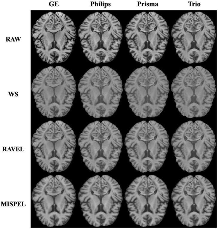
Rows and columns correspond to methods and scanners respectively.

4.5. Image Similarity

For evaluating the image similarity, we selected the mean structural similarity index measure (SSIM) which measures the similarity between two images in terms of luminance, contrast, and structure. High SSIM implies higher similarity between two images, with 1 the highest. Table 2 shows the mean and standard deviation (SD) of cross-scanner SSIM for all 6 pairwise combinations of scanners. RAW images show the lowest SSIM in all pairs, implying the existence of the scanner effect. The pairs including GE typically show low SSIMs, while Prisma-Trio shows the highest SSIM. WS and RAVEL both improve the SSIMs. Our method significantly improves the SSIMs across all combinations, implying that the harmonized scans have become more similar under this standard image quality measure.

Table 2. Structural similarity index measures (SSIM) between scanners.

Mean (and standard deviation) of the subjects is shown in each comparison. Best SSIMs across methods are in bold. All three methods show statistically significant improvement over RAW.

Methods	SSIM Between Scanners
	GE-Philips	GE-Prisma	GE-Trio	Philips-Prisma	Philips-Trio	Prisma-Trio
RAW	0.75 (0.04)	0.78 (0.04)	0.78 (0.05)	0.81 (0.03)	0.81 (0.03)	0.87 (0.04)
WS	0.79 (0.04)	0.80 (0.04)	0.80 (0.05)	0.83 (0.03)	0.83 (0.03)	0.89 (0.04)
RAVEL	0.79 (0.04)	0.80 (0.04)	0.80 (0.05)	0.83 (0.03)	0.83 (0.03)	0.88 (0.04)
MISPEL	0.84 (0.04)	0.85 (0.04)	0.86 (0.05)	0.87 (0.03)	0.87 (0.03)	0.91 (0.03)

4.6. Volumetric Similarity

The most practical benefit of harmonization is to enable accurate multi-scanner neuroimaging analyses with reduced scanner effect. Thus, it is crucial to evaluate the volumetric similarity of the neuroimaging measures which become the basis of numerous neuroimaging analyses. First, we extract the volumes of three brain tissue types: including gray matter (GM), white matter (WM), and cerebrospinal fluid (CSF). Then, we analyze their similarities across the scanners in three ways: (1) volume distributions, (2) pairwise volumetric differences, and (3) pairwise dice similarity coefficient (DSC).

4.6.1. Volume Distributions

We first look at the boxplots of the volumes of three tissue types for all scanners in Fig. 3. For our paired data, perfectly harmonized scans would show identical boxplots across all scanners and all tissue types. First, we observe the varying distributions of volumes of RAW. WS and RAVEL do not bring the boxplots together across the scanners. On the other hand, MISPEL reduces the differences in volumes across the scanners, bringing the boxplots noticeably closer to each other. We note that achieving similar volumetric distributions across the scanners is a simple but crucial requirement for any multi-scanner analysis. Otherwise, the underlying scanner effects may lead to erroneous analyses confounded by scanner types.

Figure 3. Volume distribution boxplots.

In our paired data (i.e., each subject scanned on multiple scanners with little biological differences), identical volume distributions are expected across the scanners.

4.6.2. Volumetric Differences

Our paired multi-scanner dataset allows direct comparisons of the volumes. In Table 3, we first observe the pairwise volumetric differences by computing the mean absolute difference of volumes of each tissue type between two scanners (e.g., mean of absolute difference of GM for each subject’s scan from GE and Philips). Thus, the methods aim to reduce these values compared to RAW. First, the non-zero differences for RAW data denoted the existing scanner effects. All the methods generally improve over RAW in all tissue types. In particular, MISPEL outperforms other methods in 15 out of 18 cases by large margins, often being the only statistically significant improvement. In Fig. 5, we also show root mean square error (RMSE) computing the deviation of the pairwise volume differences across subjects. The low RMSE is desired and shows the low spread of measures of scanners from each other.

Table 3. Mean absolute differences of volumes between scanners.

Bold and * indicate smallest mean across methods for each tissue and significant difference with respect to RAW, respectively.

Tissue	Methods	Mean Absolute Differences of Volumes Between Scanners
		GE-Philips	GE-Prisma	GE-Trio	Philips-Prisma	Philips-Trio	Prisma-Trio
GM	RAW	30.01 (63.57)	81.53 (70.09)	59.72 (68.41)	63.67 (26.69)	41.20 (20.84)	24.28 (15.21)
	WS	30.49 (65.35)	80.80 (71.20)	59.86 (69.71)	62.36 (26.20)*	40.47 (20.31)	23.72 (15.95)
	RAVEL	19.70 (21.29)	55.48 (23.38)	37.56 (20.23)	55.23 (25.87)*	34.75 (19.81)*	22.32 (12.99)
	MISPEL	21.12 (12.08)	10.35 (6.57)*	10.28 (7.21)*	25.08 (13.61)*	21.59 (12.95)*	8.44 (7.65)*
WM	RAW	37.73 (68.01)	77.94 (68.61)	70.84 (64.01)	41.58 (24.04)	35.78 (22.87)	14.64 (12.25)
	WS	36.22 (60.97)	69.43 (59.95)*	62.48 (56.05)*	35.13 (23.18)	30.04 (21.87)	14.50 (11.83)
	RAVEL	36.19 (65.19)	57.65 (56.27)*	56.82 (62.49)*	28.30 (23.95)*	26.72 (20.31)*	13.80 (9.29)
	MISPEL	19.03 (14.10)	14.88 (8.79)*	13.20 (12.82)*	24.80 (16.07)*	16.39 (12.33)*	14.77 (12.69)
CSF	RAW	39.16 (37.16)	27.59 (39.41)	41.05 (40.94)	19.52 (16.09)	15.43 (13.11)	15.89 (10.02)
	WS	36.72 (28.91)	24.47 (31.44)	38.15 (32.99)	19.66 (15.65)	14.24 (12.64)	15.94 (10.31)
	RAVEL	32.09 (18.92)	20.91 (19.93)	34.96 (21.49)	17.78 (16.05)	12.90 (12.50)*	16.50 (10.04)
	MISPEL	14.74 (10.10)*	11.52 (10.10)	15.78 (8.51)*	14.61 (11.75)	12.96 (9.77)	10.26 (6.61)*

Figure 5. Root mean square error (RMSE) bar plots.

In our paired data, lower values of RMSE is expected which shows lower deviation of measures across scanners.

4.6.3. Dice Similarity Coefficient (DSC)

In our final evaluation, we assess the effect of harmonization on tissue segmentation. Specifically, this provides further insight into the tissue segmentation similarity which the corresponding tissue volumes are derived from. The segmentation similarity is measured using the Dice similarity coefficient (DSC) which measures the amount of overlap between two segmentations. In this paired dataset, we would expect high overlap between the segmentations from different scanners, leading to high DSC. In Fig. 6, we see the DSC results for each tissue where MISPEL shows statistically significant improvement over RAW, WS, and RAVEL. Similar to previous evaluations, RAW GE shows weak similarity against other scanners (i.e., low DSC for GE-Philips, GE-Prisma, GE-Trio), but MISPEL effectively harmonizes GE with comparable DSC.

Figure 6. Dice similarity score (DSC) bar plots.

In our paired dataset, larger values of DSC is expected as denotes more overlap of the volume segmentations between scanners.

5. Discussion and Conclusion

We proposed MISPEL, a multi-scanner deep harmonization framework for removing scanner effects from images, while preserving their anatomical information. We also assessed scanner effects and evaluated harmonization from different aspects, using a unique paired multi-scanner dataset. The results showed that MISPEL outperformed the two well-known intensity normalization and harmonization methods, White Stripe and RAVEL, resulting more consistent tissue volumes and segmentations across all scanners.

We deem this work as a crucial first step towards our continuous harmonization study and identify several future steps to be taken. First, we believe it will be important to validate our work under other standard tissue segmentation tools such as statistical parametric mapping (SPM) [1]. While we expect the benefits to vary across the tools, such extensive assessments are crucial for a broader impact. Further, we plan to seek further qualitative assessments by expert neuroradiologists to clinically validate our work. Lastly, we aim to investigate how our harmonization framework may impact potential downstream analyses and applications such as Alzheimer’s disease detection. We optimistically expect MISPEL to improve the statistical power of various downstream statistical analyses, demonstrating the practicality and significance beyond the presented evaluative measures.

References

- [1].Ashburner John and Friston Karl J. Unified segmentation. Neuroimage, 26(3):839–851, 2005. [DOI] [PubMed] [Google Scholar]
- [2].Avants Brian B, Epstein Charles L, Grossman Murray, and Gee James C. Symmetric diffeomorphic image registration with cross-correlation: evaluating automated labeling of elderly and neurodegenerative brain. Medical image analysis, 12(1):26–41, 2008. [DOI] [PMC free article] [PubMed] [Google Scholar]
- [3].Čuklina Jelena, Pedrioli Patrick GA, and Aebersold Ruedi. Review of batch effects prevention, diagnostics, and correction approaches. In Mass Spectrometry Data Analysis in Proteomics, pages 373–387. Springer, 2020. [DOI] [PubMed] [Google Scholar]
- [4].Dewey Blake E, Zhao Can, Carass Aaron, Oh Jiwon, Calabresi Peter A, van Zijl Peter CM, and Prince Jerry L. Deep harmonization of inconsistent mr data for consistent volume segmentation. In International Workshop on Simulation and Synthesis in Medical Imaging, pages 20–30. Springer, 2018. [Google Scholar]
- [5].Dewey Blake E, Zhao Can, Reinhold Jacob C, Carass Aaron, Fitzgerald Kathryn C, Sotirchos Elias S, Saidha Shiv, Oh Jiwon, Pham Dzung L, Calabresi Peter A, et al. Deepharmony: A deep learning approach to contrast harmonization across scanner changes. Magnetic resonance imaging, 64:160–170, 2019. [DOI] [PMC free article] [PubMed] [Google Scholar]
- [6].Blake E Dewey Lianrui Zuo, Carass Aaron, He Yufan, Liu Yihao, Mowry Ellen M, Newsome Scott, Oh Jiwon, Calabresi Peter A, and Prince Jerry L. A disentangled latent space for cross-site mri harmonization. In International Conference on Medical Image Computing and Computer-Assisted Intervention, pages 720–729. Springer, 2020. [Google Scholar]
- [7].Fortin Jean-Philippe, Sweeney Elizabeth M, Muschelli John, Crainiceanu Ciprian M, Shinohara Russell T, Alzheimer’s Disease Neuroimaging Initiative, et al. Removing intersubject technical variability in magnetic resonance imaging studies. NeuroImage, 132:198–212, 2016. [DOI] [PMC free article] [PubMed] [Google Scholar]
- [8].Gorgolewski Krzysztof, Christopher D Burns Cindee Madison, Clark Dav, Halchenko Yaroslav O, Waskom Michael L, and Ghosh Satrajit S. Nipype: a flexible, lightweight and extensible neuroimaging data processing framework in python. Front Neuroinform, 5, August 2011. [DOI] [PMC free article] [PubMed] [Google Scholar]
- [9].Heinen Rutger, Bouvy Willem H, Mendrik Adrienne M, Viergever Max A, Biessels Geert Jan, and De Bresser Jeroen. Robustness of automated methods for brain volume measurements across different mri field strengths. PloS one, 11(10):e0165719, 2016. [DOI] [PMC free article] [PubMed] [Google Scholar]
- [10].Johnson W Evan, Li Cheng and Rabinovic Ariel. Adjusting batch effects in microarray expression data using empirical bayes methods. Biostatistics, 8(1):118–127, 2007. [DOI] [PubMed] [Google Scholar]
- [11].Kingma Diederik P and Ba Jimmy. Adam: A method for stochastic optimization. arXiv preprint arXiv:1412.6980, 2014. [Google Scholar]
- [12].Liu Mengting, Maiti Piyush, Thomopoulos Sophia I, Zhu Alyssa, Chai Yaqiong, Kim Hosung, and Jahanshad Neda. Style transfer using generative adversarial networks for multi-site mri harmonization. bioRxiv, 2021. [DOI] [PMC free article] [PubMed] [Google Scholar]
- [13].Modanwal Gourav, Vellal Adithya, Buda Mateusz, and Mazurowski Maciej A. Mri image harmonization using cycle-consistent generative adversarial network. In Medical Imaging 2020: Computer-Aided Diagnosis, volume 11314, page 1131413. International Society for Optics and Photonics, 2020. [Google Scholar]
- [14].Oishi Kenichi, Faria Andreia, Jiang Hangyi, Li Xin, Akhter Kazi, Zhang Jiangyang, Hsu John T, Miller Michael I, van Zijl Peter CM, Marilyn Albert, et al. Atlas-based whole brain white matter analysis using large deformation diffeomorphic metric mapping: application to normal elderly and alzheimer’s disease participants. Neuroimage, 46(2):486–499, 2009. [DOI] [PMC free article] [PubMed] [Google Scholar]
- [15].Pang Yingxue, Lin Jianxin, Qin Tao, and Chen Zhibo. Image-to-image translation: Methods and applications. arXiv preprint arXiv:2101.08629, 2021. [Google Scholar]
- [16].R Core Team. R: A Language and Environment for Statistical Computing. R Foundation for Statistical Computing, Vienna, Austria, 2020. [Google Scholar]
- [17].Ronneberger Olaf, Fischer Philipp, and Brox Thomas. U-net: Convolutional networks for biomedical image segmentation. In International Conference on Medical image computing and computer-assisted intervention, pages 234–241. Springer, 2015. [Google Scholar]
- [18].Russell T Shinohara Jiwon Oh, Nair Govind, Calabresi Peter A, Davatzikos Christos, Doshi Jimit, Henry Roland G, Kim Gloria, Linn Kristin A, Papinutto Nico, et al. Volumetric analysis from a harmonized multisite brain mri study of a single subject with multiple sclerosis. American Journal of Neuroradiology, 38(8):1501–1509, 2017. [DOI] [PMC free article] [PubMed] [Google Scholar]
- [19].Shinohara Russell T, Sweeney Elizabeth M, Goldsmith Jeff, Shiee Navid, Mateen Farrah J, Calabresi Peter A, Jarso Samson, Pham Dzung L, Reich Daniel S, and Crainiceanu Ciprian M. Australian imaging biomarkers lifestyle flagship study of ageing, and alzheimer’s disease neuroimaging initiative. statistical normalization techniques for magnetic resonance imaging. Neuroimage Clin, 6(9), 2014. [DOI] [PMC free article] [PubMed] [Google Scholar]
- [20].Shinohara Russell T, Sweeney Elizabeth M, Goldsmith Jeff, Shiee Navid, Mateen Farrah J, Calabresi Peter A, Jarso Samson, Pham Dzung L, Reich Daniel S, Crainiceanu Ciprian M, et al. Statistical normalization techniques for magnetic resonance imaging. NeuroImage: Clinical, 6:9–19, 2014. [DOI] [PMC free article] [PubMed] [Google Scholar]
- [21].Tustison Nicholas J, Avants Brian B, Cook Philip A, Zheng Yuanjie, Egan Alexander, Yushkevich Paul A, and Gee James C. N4itk: improved n3 bias correction. IEEE transactions on medical imaging, 29(6):1310–1320, 2010. [DOI] [PMC free article] [PubMed] [Google Scholar]
- [22].Wrobel J, Martin ML, Bakshi R, Calabresi PA, Elliot M, Roalf D, Gur RC, Gur RE, Henry RG, Nair G, et al. Intensity warping for multisite mri harmonization. NeuroImage, 223:117242, 2020. [DOI] [PMC free article] [PubMed] [Google Scholar]
- [23].Zhang Y, Brady M, and Smith S. Segmentation of brain mr images through a hidden markov random field model and the expectation-maximization algorithm. IEEE Trans Med Imaging, 20(1):45–57, 2001. [DOI] [PubMed] [Google Scholar]
- [24].Zhao Fenqiang, Wu Zhengwang, Wang Li, Lin Weili, Shunren Xia Dinggang Shen, Li Gang, UNC/UMN Baby Connectome Project Consortium, et al. Harmonization of infant cortical thickness using surface-to-surface cycle-consistent adversarial networks. In International Conference on Medical Image Computing and Computer-Assisted Intervention, pages 475–483. Springer, 2019. [DOI] [PMC free article] [PubMed] [Google Scholar]
- [25].Zhong Jie, Wang Ying, Li Jie, Xue Xuetong, Liu Simin, Wang Miaomiao, Gao Xinbo, Wang Quan, Yang Jian, and Li Xianjun. Inter-site harmonization based on dual generative adversarial networks for diffusion tensor imaging: application to neonatal white matter development. Biomedical engineering online, 19(1):1–18, 2020. [DOI] [PMC free article] [PubMed] [Google Scholar]
- [26].Zuo Lianrui, Blake E Dewey Aaron Carass, Liu Yihao, He Yufan, Calabresi Peter A, and Prince Jerry L. Information-based disentangled representation learning for unsupervised mr harmonization. In International Conference on Information Processing in Medical Imaging, pages 346–359. Springer, 2021. [Google Scholar]