Quantitative Characterization of the Human Retinotopic Map Based on Quasiconformal Mapping

Abstract

The retinotopic map depicts the cortical neurons’ response to visual stimuli on the retina and has contributed significantly to our understanding of human visual system. Although recent advances in high field functional magnetic resonance imaging (fMRI) have made it possible to generate the in vivo retinotopic map with great detail, quantifying the map remains challenging. Existing quantification methods do not preserve surface topology and often introduce large geometric distortions to the map. In this study, we developed a new framework based on computational conformal geometry and quasiconformal Teichmüller theory to quantify the retinotopic map. Specifically, we introduced a general pipeline, consisting of cortical surface conformal parameterization, surface-spline-based cortical activation signal smoothing, and vertex-wise Beltrami coefficient-based map description. After correcting most of the violations of the topological conditions, the result was a “Beltrami coefficient map” (BCM) that rigorously and completely characterizes the retinotopy map by quantifying the local quasiconformal mapping distortion at each visual field location. The BCM provided topological and fully reconstructable retinotopic maps. We successfully applied the new framework to analyze the V1 retinotopic maps from the Human Connectome Project (n=181), the largest state of the art retinotopy dataset currently available. With unprecedented precision, we found that the V1 retinotopic map was quasiconformal and the local mapping distortions were similar across observers. The new framework can be applied to other visual areas and retinotopic maps of individuals with and without eye diseases, and improve our understanding of visual cortical organization in normal and clinical populations.

Graphical Abstract

1. Introduction

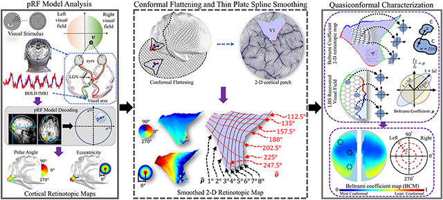
The mammalian visual cortex contains multiple continuous topographic representations of the visual field within its folded anatomical structure (Thompson et al., 1950; Cowey, 1964; Hubel and Wiesel, 1965; Tusa et al., 1978; Horton and Hoyt, 1991; Wang and Burkhalter, 2007). Although the exact shape of visual input on the retina is not preserved in cortical representations, neurophysiology studies (Talbot and Marshall, 1941; Daniel and Whitteridge, 1961) have shown that cortical representations can be unfolded, stretched, compressed, shifted, and rotated (without cutting/tearing) such that they are aligned to the exact shape of the visual input. In other words, although cortical representations of visual input on the retina do not preserve metric (distance) properties, they preserves local neighborhood geometric relationships (Sereno et al., 1995; Engel et al., 1997; Swindale et al., 2000; Warnking et al., 2002b). More specifically, neighboring points on the cortical surface should have neighboring retinal visual coordinates (Wandell et al., 2007). We adopted the term topology preserving to refer to the preservation of neighborhood relationships of the input in the output space (Ho-Phuoc and Guerin-Dugue, 2009). Finally, the result is known as the retinotopic representation in the visual system (Daniel and Whitteridge, 1961; Horton and Hoyt, 1991). Recent advances in functional magnetic resonance imaging (fMRI), a non-invasive technique for measuring human brain activity, have made in vivo retinotopic mapping of the human visual cortex a standard technology in visual neuroscience (Schneider et al., 1993; Sereno et al., 1995; Tootell et al., 1995; DeYoe et al., 1996; Engel et al., 1994, 1997; Brewer et al., 2005). In many studies, Blood-Oxygenation-Level-Dependent (BOLD) fMRI activation data are analyzed with the population receptive field (pRF) model (Dumoulin and Wandell, 2008) to estimate the center and size of the receptive field of each voxel on the cortical surface (Fig. 1). The retinotopic map generated from such analysis has contributed tremendously to our understanding of the human visual system (Schwarzkopf et al., 2011; Wandell and Winawer, 2011; Brewer and Barton, 2014; Michel et al., 2013; Morland et al., 2001; Kammen et al., 2016). On the other hand, although numerous studies have been devoted to generating and investigating properties of the retinotopic map, most of them have taken an experimental approach. Questions regarding the exact nature of the geometric transformations in retinotopic mapping and how human visual system “recovers” the shape of visual input from such transformations remain open. A complete quantitative characterization of the retinotopic map is the key to addressing these questions.

Figure 1:

Illustration of the procedure for generating the retinotopic map from functional magnetic resonance imaging (fMRI) with the population receptive field (pRF) model (Dumoulin and Wandell, 2008): (a) moving visual patterns for retinotopy experiments, which consist of checkerboard textured expanding rings and rotating wedges; (b) the visual field and the visual pathway to the primary visual area V1 on the cortex is systematically stimulated; (c) voxel-wise BOLD fMRI time series signal are analyzed using the pRF model to predict the centers of the receptive field and coregistered onto the triangle mesh surface representation of the cortical surface in (d,e). The color mapped degree of visual field eccentricity (d) and polar angle (e) on the primary visual cortex (V1) results are shown with key anatomical landmarks labeled (vertical and horizontal meridian).

The relatively few quantitative retinotopic studies (Balasubramanian et al., 2002; Schira et al., 2007, 2009; Benson et al., 2012, 2014; Benson and Winawer, 2018) have mostly focused on a template-based fitting approach, which was first used to quantify “cortical magnification” as a function of eccentricity and polar angle in animals (Daniel and Whitteridge, 1961; Schwartz, 1977, 1980) before being later refined to describe the human retinotopic map (Schira et al., 2007, 2009). In this approach, a 2-dimensional angle-preserving algebraic model (Schwartz, 1977, 1980) or its improved non-conformal variants (Balasubramanian et al., 2002; Schira et al., 2007, 2009) are used to model the retinotopy data on the cortical surface. The latter approaches (Balasubramanian et al., 2002; Schira et al., 2007, 2009) found that empirical human retinotopic maps are best fit with quasiconformal rather than conformal templates. The templates were constructed from (1) the “log-transform” function (Schwartz, 1977, 1980) which is conformal and (2) extended with the “double-sech” (Schira et al., 2007) shearing function which locally adjusted the “log-transform” to better fit the empirical retinotopic maps. Because the templates are constrained by only a few parameters, finding the optimal template of a given retinotopic map by regression is greatly simplified. However, because the templates were restricted to only conformal mappings with shearing approximated by the “double-sech” at eccentricity and polar angle locations, the quantification of retinotopic maps are biased. Because angle distortion bias were introduced in the modeling process, it is unclear how much of the angle distortions are actually in the original retinotopic maps. It is important to note that current quantitative models of human retinotopic maps (Schira et al., 2007, 2009) are extended from primate models whose “cortical magnification” quantification in visual area V1 has been reported to be approximately conformal (i.e., angle-preserving) (Van Essen et al., 1984; Schwartz, 1985; Tootell, 1985). However, there has been no rigorous numerical method to estimate the conformality (i.e., angle-preserving property) of the human retinotopic map (Schira et al., 2007), and the cortical surface flattening procedure often introduces additional angle distortions (Schwartz, 1977; Schira et al., 2007, 2009; Benson et al., 2012). With very few parameters, the algebraic model or its variants can only be used to approximate the global average shape of the retinotopic map; it cannot account for the well-known asymmetry across the horizontal and vertical meridians (Liu et al., 2006) and significant local variations across individual observers. Moreover, the results cannot be used to accurately reconstruct the original retinotopic mapping function under suitable boundary conditions. Namely, it cannot be used to accurately project cortical activation back to the visual field.

To address these challenges, we developed a computational framework to quantify the mapping from the 2-dimensional cortical surface to the visual field, based on the output of the pRF model analysis of the fMRI retinotopic data (Sereno et al., 1995; DeYoe et al., 1996; Tootell et al., 1995, 1998; Hansen et al., 2004). Although traditionally the retinotopic map refers to the mapping from the retina to visual cortex, we use the term retinotopic map in the opposite direction in this study. Our new framework is based on computational conformal geometry (Jin et al., 2018) and quasiconformal Teichmüller theory (Gardiner and Lakic, 2000). It produces a rigorous mathematical characterization of the retinotopic map that can fully describe its global and local properties, and under suitable boundary conditions, be used to reconstruct the original retinotopic mapping function. Because topological relationships are reciprocal, our conclusion also holds for the mapping from the retina to visual cortex (Balasubramanian et al., 2002).

In our framework, we introduced Beltrami coefficient (BC) to characterize the degree of conformality in the retinotopic map. In conformal mapping, local regions on one surface (circles in Fig. 2 (a)) are mapped onto local regions on another surface with the same local metric up to a scaling factor (different sized circles in Fig. 2 (c)). In quasiconformal mapping, local regions on one surface are mapped onto local regions on another surface with a bounded change to the local metric (different sized ellipses in Fig. 2 (b)). Both types of mappings preserve topology; that is, although the shape of each local region (a circle) is stretched, compressed, shifted, or rotated, its relative position to nearby local regions (nearby circles or ellipses) remains fixed. The BC for each local region (a circle), defined as a complex-valued local measure of angle distortion μ satisfying ∥μ∥_∞ < 1. It describes the “distortion” of f(z) from the circle z = u⁽¹⁾ + iu⁽²⁾ to to an ellipse, as illustrated in Fig. 2 (d). If the BC is everywhere zero, the mapping is conformal; if it is different from zero, the mapping is quasiconformal. Therefore, the BC provides a metric to test if the retinotopic map is conformal or quasiconformal and quantifies the “distortion” in each local region of the cortical surface. We call the collection of BCs computed on the 2-dimensional retinotopic map of primary visual cortex (V1) the Beltrami coefficient map (BCM) of V1.

Figure 2:

Illustration of conformal mapping, quasiconformal mapping, and Beltrami coefficient quantification. (a) The source surface is the 2-D retinotopic map in V1; (b) quasiconformal mapping to the target visual field; (c) conformal mapping to the target visual field; (d) Beltrami coefficient (BC) quantification. The BC is the eccentricity of the ellipse in (d). It measures the “distortion” from “circles to circles” (conformal) or “circles to ellipses” (quasiconformal) computed between each local region z = u⁽¹⁾ + iu⁽²⁾ on the retinotopic map to the associated mapped region w = f(z) = v⁽¹⁾ + iv⁽²⁾ on the visual field. On the triangle mesh representations of cortical anatomy, BC is computed on each triangle.

A major mathematical property of the BCM is that the original mapping function from which the BCM was computed can be reconstructed under suitable boundary conditions. According to quasiconformal Teichmüller theory (Gardiner and Lakic, 2000), under suitable normalization, there is a one-to-one correspondence between the BCM and quasiconformal homeomorphisms. To reconstruct the original retinotopic mapping function from the BCM, we constructed and solved a system of equations called the Linear Beltrami Solver (LBS) (Lui et al., 2013). By solving the LBS with appropriate boundary conditions, we can completely recover the visual input on the retina from the 2-dimensional BCM. Because the sequence of mappings from the cortical surface to the visual field are unique, we can accurately project brain activations on V1 back to the visual field by reconstructing the retinotopic mapping function from the BCM followed by the conformal maping that was used to parameterize the cortical surface to the planar disk.

The BCM translates the retinotopic map into a complete quantitative characterization, making it possible to rigorously test the conformality of the retinotopic map. The quantitative description will make it possible to apply many data analytic methods to analyze the retinotopic map at both individual and population levels. Characterizing the exact nature of the geometric transformations in retinotopic mapping across multiple visual areas may also help address one of the fundamental questions in perception: how can we perceive a veridical visual world in the face of the various geometric distortions in retinotopic representations? The new framework can be applied to various visual areas and retinotopic maps of individuals with and without eye diseases, and shed new light on the functional organization of the visual system.

2. Methods and Materials

Our retinotopic map characterization is based on the Beltrami coefficient description of quasiconformal maps. We begin with the theory of quasiconformal maps and the numerical schemes to compute the Beltrami coefficient (BC) and reconstruct quasiconformal mappings with the BC on discrete surfaces (Sec. 2.1). We then provide a brief overview of our processing pipeline (Sec. 2.2) before explaining the complete details at each major step: (1) generating the retinotopic map using the pRF model (Sec. 2.3); (2) conformal flattening of the visual cortical surface to planar disk domain (Sec. 2.4); (3) thin plate spline smoothing of retinotopy data (Sec. 2.5); and (4) computing the Beltrami coefficient map (BCM) for the transformation between the retina and V1 (Sec. 2.6). We also address how we can use the BCM encoding to reconstruct the visual field activations (Sec. 2.7). The retinotopic data we analyzed in this study and our released software package are reported in Sec. 2.8.

2.1. Theoretical Background and Numerical Scheme

In this section, we briefly introduce the most relevant theoretical background in quasiconformal mapping (Ahlfors, 1966) and the set of equations to numerically compute the Beltrami coefficient description on discrete triangle mesh surfaces. We then introduce the linear Beltrami solver (Lui et al., 2013) to recover the unique quasiconformal mapping function from its Beltrami coefficient description.

2.1.1. Beltrami Equation

A conformal map is a function that locally preserves angles (Jin et al., 2018). Quasiconformal maps are generalization of conformal maps, which are orientation preserving homeomorphisms between Riemann surfaces with bounded conformality distortion. Mathematically, given two Riemann surfaces S₁, $S_2\in \mathbb{C}$, where $\mathbb{C}$ is the complex plane, a map f : S₁ → S₂ is quasiconformal if it has continuous partial derivatives and satisfies the Beltrami equation,

$$\frac{\partial f}{\partial \overline{u}}=u_f\frac{\partial f}{\partial u},\forall u=u^{(1)}+i{u}^{(2)}$$ (1)

where μ_f is the Beltrami coefficient with ∥μ_f∥_∞ < 1. When μ_f = 0, f is conformal.

2.1.2. The “one-to-one” Relationship

Given a quasiconformal map f, one can uniquely compute the Beltrami coefficient μ_f according to Eq. 1. The following quasiconformal theorem establishes that we can recover a unique 2-D quasiconformal map f from a given Beltrami coefficient μ, up to normalization.

Theorem 2.1. (Ahlfors, 1966) Given a Lebesgue measurable μ with ∥μ_f∥_∞ < 1, and three given target points (e.g., given the value of f(0), f(1), f(∞)), then a unique quasiconformal map f can be found by solving the Beltrami equation (Eq. 1).

If the Beltrami coefficient and 3 fixed points are given, we can find the unique f by separating the Beltrami equation into two real-valued partial differential equations and solving them respectively. Suppose the given Beltrami coefficient is μ = η + iτ. To recover the map f = v⁽¹⁾ + iv⁽²⁾, we set the right hand side of Eq. 1 with μ = η + iτ and apply the complex derivative definitions: $\frac{\partial f}{\partial \overline{u}}=\frac{1}{2}\frac{\partial f}{\partial u^{(1)}}+\frac{i}{2}\frac{\partial f}{\partial u^{(2)}}$, and $\frac{\partial f}{\partial u}=\frac{1}{2}\frac{\partial f}{\partial u^{(1)}}-\frac{i}{2}\frac{\partial f}{\partial u^{(2)}}$, to get

$$\left(\frac{\partial f}{\partial u^{(1)}}+i\frac{\partial f}{\partial u^{(2)}}\right)∕\left(\frac{\partial f}{\partial u^{(1)}}-i\frac{\partial f}{\partial u^{(2)}}\right)=\eta +i\tau .$$ (2)

After reorganizing and eliminating v⁽²⁾, Eq. 2 can be written as,

$$\nabla \cdot (A\nabla v^{(1)})=0,$$ (3)

where $A=\left(\begin{array}{cc}\hfill {\alpha }_1\hfill & \hfill {\alpha }_2\hfill \\ \hfill {\alpha }_2\hfill & \hfill {\alpha }_3\hfill \end{array}\right)$ is a 2-by-2 square matrix with value

$$\begin{gathered} {\alpha }_1=\left((\eta -1{)}^2+{\tau }^2\right)∕\left({\eta }^2+{\tau }^2-1\right), \\ {\alpha }_2=(-2\tau )∕\left({\eta }^2+{\tau }^2-1\right), \\ {\alpha }_3=\left(1+2\eta +{\eta }^2+{\tau }^2\right)∕\left({\eta }^2+{\tau }^2-1\right). \end{gathered}$$

By solving the differential equation (Eq. 3) with Dirichlet boundary conditions (which is governed by the 3 fixed points), we obtain v⁽¹⁾. Similarly, if we eliminated v⁽¹⁾, we have ∇ · A∇v⁽²⁾ = 0, which can be solved to obtain v⁽²⁾.

Because the quasiconformal map f and the associated Beltrami coefficient μ has a one-to-one relationship with 3 fixed points, we can encode the function f by μ_f. Effectively, we can characterize and manipulate f by μ_f. This main idea has been utilized in our prior work (e.g., Yu et al., 2017; Zhang et al., 2019) and was applied twice in the current work.

2.1.3. Beltrami Coefficients on Discrete Surfaces

Since the cortical surfaces in this work are represented with triangle meshes, we use finite element method to numerically approximate the computation of Beltrami coefficients and reconstruction of quasiconformal maps.

Let T_i,j,k = [u_i, u_j, u_k] be a triangle on the parametric space consisting of vertices u_i, u_j and u_k, we denote the triangle area by ∣[u_i, u_j, u_k]∣. The discrete map provides their visual coordinates v_i, v_j and v_k on the vertices of T_i,j,k, respectively. We extend the domain and approximate the mapping v = f(u) within the triangle T_i,j,k by linear interpolation,

$$v_{T_{i,j,k}}=f(u){\mid }_{T_{i,j,k}}=B_i(u)v_i+B_j(u)v_j+B_k(u)v_k,$$ (4)

where u is an arbitrary point in triangle T_i,j,k, and B_i(u), B_j(u), B_k(u) are called the barycentric coefficients. The barycentric coefficient B_i is defined as the area ratio of the triangle [u, u_j, u_k] to the area of triangle [u_i, u_j, u_k], i.e., B_i = ∣[u, u_j, u_k]∣/∣[u_i, u_j, u_k]∣. Similarly, B_j = ∣[u_i, u, u_k]∣/∣[u_i, u_j, u_k]∣ and B_k = ∣[u_i, u_j, u]∣/∣[u_i, u_j, u]∣. Let n be the unit normal of T_i,j,k, then the discrete gradient of f in triangle T_i,j,k can be written as

$$\nabla f(u){\mid }_{T_{i,j,k}}=\left(\frac{\partial f}{\partial u^{(1)}},\frac{\partial f}{\partial u^{(2)}}\right)=v_i\nabla B_i+v_j\nabla B_j+v_k\nabla B_k,$$ (5)

where ∇B_i = s_i/ (2 ∣[u_i, u_j, u_k]∣) and s_i = n×(u_j-u_k). Similarly, s_j = n×(u_k–u_i) for ∇B_j = s_j/(2 ∣[u_i, u_j, u_k]∣), and s_k = n × (u_i – u_j) for ∇B_k = s_k/(2 ∣[u_i, u_j, u_k]∣). Fig. 3 (a) illustrates s_i, s_j, and s_k in a given triangle T_i,j,k.

Figure 3:

Illustration of the discrete gradient and discrete divergence computation. (a) The triangle T_i,j,k, and vectors s_i, s_j, and s_k in the discrete gradient computation (Note that the normal n is not shown here but it points outside of the page from the triangle); (b) the discrete divergence of vertex u_i is computed by the average out-flux of vector filed G within its dual polygon D (Meyer et al., 2003).

Substituting the result of ∂f/∂u⁽¹⁾ and ∂f/∂u⁽²⁾ from Eq. 5 into Eq. 2, we can numerically compute the Beltrami coefficient, which is a constant for each triangle.

2.1.4. Discrete Quasiconformal Map Reconstruction

Given the “one-to-one” relationship between Beltrami coefficients and quasiconformal maps, several numerical schemes (e.g., Lui et al., 2012; Zeng et al., 2012), including our own work (Yu et al., 2017; Zhang et al., 2019), have been introduced to solve Eq. 2 and reconstruct discrete quasiconformal maps with Beltrami coefficients. In this work, we adopted the linear Beltrami solver (LBS) (Lui et al., 2013) for the quasiconformal map reconstruction because of its numerical efficiency. Its solution is a unique quasiconformal map.

By definition, the divergence on a 2-D vector field G = (G⁽¹⁾, G⁽²⁾) in the Euclidean planar space is defined as,

$$\nabla \cdot \mathit{G}=\left(\frac{\partial }{\partial u^{(1)}},\frac{\partial }{\partial u^{(2)}}\right)\cdot (G^{(1)},G^{(2)}{)}^T=\frac{\partial G^{(1)}}{\partial u^{(1)}}+\frac{\partial G^{(2)}}{\partial u^{(2)}}.$$ (6)

Numerically computing the divergence on the discrete gradient approximation is not accurate enough. Instead, we use Stoke’s theorem to approximate the divergence of a triangle mesh vertex. As shown in Fig. 3 (b), it is the average out-flux of vector field G of its dual polygon D. The vertex-dual is a polygon constructed from the circumcenters of the attached triangles. Mathematically, the discrete divergence (Meyer et al., 2003) is defined as,

$$\nabla \cdot \mathit{G}(u_i)=\frac{1}{\mid D\mid }{\int }_{\partial D}\mathit{G}\cdot (\mathit{n}\times d\mathit{l})=\frac{1}{\mid D\mid }\sum _{[u_i,u_{\alpha },u_{\beta }]\in N(u_i)}{\mathit{G}}_{[u_i,u_{\alpha },u_{\beta }]}\cdot \frac{{\mathit{s}}_i}{2},$$ (7)

where N(u_i) is the neighbouring (attaches to u_i) triangle set of vertex u_i, ∣D∣ is the area of the dual polygon, ∂D is the boundary of D, and G_[ui,uα,uβ] is the vector value on triangle [u_i, u_α, u_β] and s_i = n × (u_α – u_β) as defined earlier.

With the definitions of both discrete gradient and discrete divergence, we can rewrite Eq. 3 in a matrix form as LV⁽¹⁾ = 0 and LV⁽²⁾ = 0, where ${\mathit{V}}^{(1)}={\left[v_1^{(1)},v_2^{(1)},\dots ,v_W^{(1)}\right]}^T$, ${\mathit{V}}^{(2)}={\left[v_1^{(2)},v_2^{(2)},\dots ,v_W^{(2)}\right]}^T$, where W is the number of vertices, and L is the generalized Laplacian matrix. As an elliptic partial differential equation, the generalized Laplacian equation enjoys strong numerical stability.

The matrix form LV⁽¹⁾ = 0 and LV⁽²⁾ = 0 each contains W number of equations. For the i-th equation, L_i,j is the coefficient of the variables $v_j^{(1)}$, $L_{i,1}{v}_1^{(1)}+L_{i,2}{v}_2^{(1)}+\cdots +L_{i,W}{v}_W^{(1)}=0$ and $v_j^{(2)}$, $L_{i,1}{v}_1^{(2)}+L_{i,2}{v}_2^{(2)}+\cdots +L_{i,W}{v}_W^{(2)}=0$. We explicitly calculate L_i,j as follows,

$$L_{i,j}=\{\begin{array}{c}\sum _{[{\mathit{u}}_{\mathit{i}},{\mathit{u}}_{\mathit{j}},{\mathit{u}}_{\mathit{k}}]\in N(i)}\frac{(A{\mathit{s}}_{\mathit{j}})\cdot {\mathit{s}}_{\mathit{i}}}{\mid [{\mathit{u}}_{\mathit{i}},{\mathit{u}}_{\mathit{j}},{\mathit{u}}_{\mathit{k}}]\mid },\text{if}j\ne i\hfill \\ -\sum _{k\ne i}{L}_{i,k},\text{if}j=i\hfill \\ 0,\text{otherwise}\hfill \end{array}\phantom{\}}$$ (8)

If we let I and B be the free and fixed vertex indices respectively, the discrete quasiconformal map f can be obtained by solving the linear equations $L_{I,I}{\mathit{V}}_I^{(1)}=-L_{I,B}{\mathit{V}}_B^{(1)}$ and $L_{I,I}{\mathit{V}}_I^{(2)}=-L_{I,B}{\mathit{V}}_B^{(2)}$. ${\mathit{V}}_B^{(1)}$ and ${\mathit{V}}_I^{(1)}$ are sub-vectors of V⁽¹⁾ composed of $v_i^{(1)}$ for i ∈ B and i ∈ I respectively. ${\mathit{V}}_B^{(2)}$ and ${\mathit{V}}_I^{(2)}$ are similarly defined. The matrix L_I,B is a sub-matrix of L composed of L_i,j, for i ∈ I and j ∈ B. The matrix L_I,I is similarly defined.

2.2. System Pipeline

This section briefly introduces the proposed Beltrami coefficient map (BCM) quantification pipeline for human retinotopic maps. The major steps to compute the BCM for a given retinotopic map are summarized in Fig. 4 and Alg. 1. The computational details are described in Secs. 2.3-2.6. There are 4 major components: (1) generating the retinotopics map from BOLD fMRI data with the pRF model (Dumoulin and Wandell, 2008); (2) computing the unit disk conformal parameterization of the primary visual cortex (V1); (3) smoothing the retinotopic map to ensure that it preserves topology despite the low spatial resolution and low signal-to-noise ratio of retinotopy data; and (4) quantifying the mapping between the retina and the primary visual cortex (V1) using the Beltrami coefficient. The output of the pipeline is the BCM.

Figure 4:

Illustration of our retinotopic map quantification pipeline, inputs, and output. (a) The retinotopic map on the 3-dimensional cortical surface is generated by applying the pRF model on the BOLD fMRI time series signal; (b,c) conformal flattening of visual cortical surfaces to parameter domain D_V1; (d, e) thin plate spline (Duchon, 1977) smoothing of retinotopy data {(ρ, θ)} on the parameter domain D_V1; (f,g) computing the Beltrami coefficient map from the smoothed retinotopy data {($\widehat{\rho }$, $\widehat{\theta }$)} and the parameter coordinates {(u⁽¹⁾, u⁽²⁾)}. The obtained (g) Beltrami coefficient map (BCM) is a complete description of the retinotopic map.

2.3. Population Receptive Field (pRF) Decoding

Given the set of voxel-wise BOLD fMRI time series signal resulting from visual field stimulation of an observer, the population receptive model (pRF) (Dumoulin and Wandell, 2008; Kay et al., 2013b) will predict for each voxel, the center v and size $\sigma \in {\mathbb{R}}^{+}$ of its receptive field on the 2-D visual field, as illustrated in Fig. 5 (a). If we let the stimulation pattern be s(v; t) as shown in Fig. 5 (b), where $v=\left(v^{(1)},v^{(2)}\right)\in {\mathbb{R}}^2$ is located on the visual field, then the predicted fMRI signal can be written as (Fig. 5 (c,d)),

$$p(v,\sigma )=\beta \left(\int r(v^{\prime };v,\sigma )s(t,v^{\prime })d{v}^{\prime }\right)\ast h(t)$$ (9)

where, β is a coefficient that converts the units of response to the unit of fMRI activation, r (v′; v, σ) is a predefined model of the neuronal response around v, and h(t) is the hemodynamic function (a model of the time course of neuronal activation to a stimulus, Fig. 5 (c)).

Figure 5:

Overview of the population receptive field (pRF) model (Dumoulin and Wandell, 2008). (a) The parameters (v,σ) predicted by the pRF model for the voxel-wise time series BOLD fMRI signal; (b) visual stimulus for generating retinotopic maps. The output (d) BOLD fMRI signal p(t) is modeled as a convolution of the (c) stimulus activation and the hemodynamic function h(t).

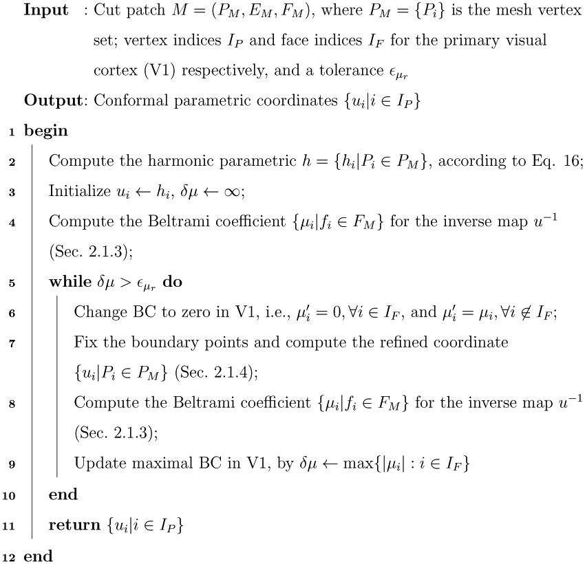
Algorithm 1: Beltrami Coefficient Map (BCM) Computation Pipeline.

The parameters v and σ were obtained by minimizing the prediction error,

$$(v,\sigma )=\text{arg}\underset{(v,\sigma )}{\text{min}}\mid p(v,\sigma )-y(P){\mid }^2.$$ (10)

The retinotopic mapping of the entire visual cortex was obtained when (v, σ) is solved for every point on the cortical surface. Usually, r(v′; v, σ) is chosen to be a 2D Gaussian kernel, i.e.,

$$r(v^{\prime };v,\sigma )\propto \text{exp}(-\frac{(v^{(1)}-v^{\prime (1)}{)}^2+(v^{(2)}-v^{\prime (2)}{)}^2}{2{\sigma }^2}).$$ (11)

The quality of fit by the pRF model was evaluated by computing the variance explained R² on each voxel,

$$R^2=1-\frac{\int (\widehat{y}-\overline{y}{)}^{2}dt}{(y-\overline{y}{)}^{2}dt}.$$ (12)

where $\overline{y}$ is the mean of the ground truth data y.

After all voxels were decoded, we assigned the predicted retinotopic coordinates $v_i=\left(v_i^{(1)},v_i^{(2)}\right)$ at each point x_i ∈ P. Because retinotopic studies traditionally used polar angle coordinates to refer to positions in the visual field, we also kept this convention and used (ρ_i, θ_i) for the estimated pRF location of v, where ρ_i was the eccentricity of the estimated pRF location, θ_i was the angle of the estimated pRF location, $v_i^{(1)}={\rho }_i\cos ({\theta }_i)$, $v_i^{(2)}={\rho }_i\sin ({\theta }_i)$, and location (0, 0) was the center of the visual field.

2.4. Conformal Flattening of Primary Visual Area (V1)

Similar to other quantitative retinotopic studies (e.g., Balasubramanian et al., 2002; Schira et al., 2007, 2009; Benson et al., 2012, 2014; Benson and Winawer, 2018), the main parameter space is the flattened visual cortical surface in this work. Different from prior work, we pursued a conformal mapping from the visual cortical surface to a planar disk and later used it to evaluate whether the human retinotopic map is conformal (i.e., angle preserving). To achieve accurate conformal mapping, we designed a robust algorithm to flatten the primary visual area (V1) to the planar disk. Fig. 6 illustrates the pipeline. We started with Loop’s subdivision algorithm (Loop, 1987) to increase the triangular mesh resolution (Fig. 6 (a)). With the cortical spherical parameterization computed by FreeSurfer ((Fischl, 2012), Fig. 6 (b), we smoothed the subdivided cortical surface with the spherical harmonic basis functions ((Gu et al., 2004; Chung et al., 2007), Fig. 6 (c)). Further, we cut out the visual cortical area (Fig. 6 (d)) and computed a harmonic map, h, to a planar disk (Jin et al., 2018). Finally, by adjusting the Beltrami coefficients of the harmonic map, we refined the disk-to-disk map, r and the resulting composite map c = r ∘ h is a conformal mapping from the visual cortical surface to the planar disk ((Choi and Lui, 2015), Fig. 6 (f)).

Figure 6:

Pipeline of conformal flattening of primary visual area (V1). (a) Cortical surface subdivision; (b) spherical parameterization computed with FreeSurfer (Fischl, 2012); (c) with the spherical coordinates, spherical harmonic (SPHARM) basis functions are used to smooth the vertex positions of newly added subdivision vertices; (d) the cut-off visual cortical surface patch (the region of interest) containing primary visual area (V1); (e) harmonic map, h, of the region of interest to a planar disk, including h(V₁); (f) the resulting conformal map of the region of interest, c = r ∘ h, including c(V₁); the checkerboard texture inferred from the conformal map is applied on the region of interest on the original cortical surface.

Algorithm 2: Conformal parametrization of primary visual cortex (V1).

2.4.1. Surface Subdivision and Visual Coordinate Interpolation

The current research focused on visual cortical area, specifically, V1 visual area. To reduce numerical errors in geometry processing, we subdivided the V1 surface area to obtain a denser triangle mesh for improved geometry computation accuracy (Loop, 1987). Namely, for each triangle on the original mesh, we constructed an extra triangle using the midpoints of its edges. In total, the surface subdivision split each original triangle into four triangles, as illustrated in Fig. 6 (a) where a triangle is divided divided into four triangles, with a newly added red triangle. Other vertex properties, such as spherical parameterization coordinates are also linearly interpolated on the newly added vertices.

We then slightly smoothed the vertex positions of the new mesh by spherical harmonic smoothing. Suppose the vertex coordinates V⁽¹⁾, V⁽²⁾, and V⁽³⁾ are functions defined on the unit sphere (i.e., $V_i^{(1)}=V^{(1)}({\Theta }_i,{\Phi }_i)$, $V_i^{(2)}=V^{(2)}({\Theta }_i,{\Phi }_i)$, and $V_i^{(3)}=V^{(3)}({\Theta }_i,{\Phi }_i)$, where (Θ_i, Φ_i) is the spherical polar angle and azimuthal angle of parameterization coordinates), then we can approximate continuous functions of them with spherical harmonic basis functions,

$${\widehat{V}}^{(i)}(\Theta ,\Phi )=\sum _{\ell =0}^L\sum _{m=-\ell }^{\ell }{c}_{\ell }^{m,i}{Y}_{\ell }^m(\Theta ,\Phi ),$$ (13)

where i = 1, 2, 3, $c_{\ell }^{m,i}$ is the spherical harmonic coefficient, and $Y_{\ell }^m$ is the orthonormal spherical harmonic basis function (Vilenkin, 1968). The spherical coefficients, $c_{\ell }^{m,i}$, are estimated by $c_{\ell }^{m,i}=<V^{(i)},Y_{\ell }^m>$, where the inner product is defined as

$$<V^{(i)},Y_{\ell }^m>={\int }_0^{\pi }\left[{\int }_0^{2\pi }{V}^{(i)}(\theta ,\varphi )\overline{Y_{\ell }^m(\theta ,\varphi )}d\varphi \right]\sin \theta d\theta .$$ (14)

On surface meshes, the coefficients are approximated in the least-squares sense (Brechbühler et al., 1995; Styner et al., 2006).

Here, we used Freesurfer’s (Fischl, 2012), spherical inflation (unit sphere, Fig. 6 (b)) coordinates as the surface parameterization coordinates (Θ, Φ). The coefficients $c_{\ell }^m$ can be efficiently computed by discrete weighted SPHARM iterative algorithm (Chung et al., 2007). After applying a low pass filter on the obtained coefficients $c_{\ell }^m$, the coefficients of high frequency basis are set to zero ($c_{\ell }^m=0$) to get a smooth surface. Fig. 6 (c) shows reconstructured cortical surfaces with l = 5, 15, 25, 100, respectively. Empirically, we found that the differences between the original cortical and reconstructed surfaces are stable when l > 100. Therefore, we used l = 100 in the current work.

On the smoothed surface, we linearly interpolated the pRF parameters on all the new points. To avoid discontinuity of visual polar angle on the positive x-axis, we first transformed the visual coordinates to the Cartesian coordinates, applied the linear interpolation on the Cartesian visual coordinates, and back transformed the Cartesian visual coordinates into polar angle coordinates.

2.4.2. Visual Surface Area Patch Selection and Cutting

After up-sampling the spatial resolution of the cortical surface with subdivision, we cut a region of interest that encloses the primary visual cortex (V1). We begin by roughly choosing a point corresponding to the visual fovea as the center. We then computed the geodesic distance (Sethian, 1999) from all cortical points to this center point. We selected the mesh portion that lies within the predefined geodesic threshold (g_th = 90mm in this work). The resulting mesh patch is illustrated as the checkerboard texture region in Fig. 6 (d). Later, we conformmally map this geodesic patch to a unit disk as shown in Fig. 6 (f).

2.4.3. Conformal Mapping of Primary Visual Cortical Surface

We used the conformal disk parameterization, $c:M\to \mathbb{D}$, to flatten the cortical surface patch M to the disk domain $\mathbb{D}$, which are the checkerboard region in Fig. 6 (d) and the disk in Fig. 6 (f) respectively. Namely, the input patch is an open boundary genus-0 surface (the cut patch in Sec. 2.4.2) and the output is its conformal mapping to the unit disk.

To achieve quality conformal mapping results, we introduced a new algorithm to achieve conformal mapping of the V1 retinotopic map on the unit disk $\mathbb{D}$. First, we applied the harmonic mapping ((Jin et al., 2018), Fig. 6 (e)) to the unit disk as the initial mapping. This guaranteed that the boundary of M is on the boundary of the $\mathbb{D}$. Second, we iteratively optimized the conformality of the patch until the BC within V1 is within the predefined error ∥μ∥_∞ ≤ ϵ_μ.

Harmonic Maps. The harmonic map $h:M\to \mathbb{D}$ can be found by minimizing the following energy (Gu et al., 2004)

$$E(h)={\int }_M\mid \nabla h{\mid }^{2}d{v}_M.$$ (15)

Namely, the harmonic map for disk like surfaces $h:M\to \mathbb{D}$ can be found by setting ∇E(h) = 0, which yields the Laplace equation (Wang et al., 2007)

$$\{\begin{array}{cc}\Delta h(u{)}_M\hfill & =0,\hfill \\ \hfill & \hfill \\ h{\mid }_{\partial M}\hfill & =g,\hfill \end{array}\phantom{\}}$$ (16)

where Δ is the Laplacian operator and g : ∂M → ∂G can be given by the arc length parameterization.

In the discrete case, the Laplace equation ∇h (u) = 0 in Eq. 16 is a sparse linear system, written as L^hh = 0. The matrix element $L_{i,j}^h$ is the special case of Eq. 8 when A is the identity matrix. Here, we set the boundary vertices by its boundary length. Each vertex $\{v_i{\}}_{i=0}^{n-1}$ is mapped to the unit circle according to the ratio of the edge lengths along the boundary loop. The harmonic map h is efficiently obtained by solving the linear system (Eq. 8) (Wang et al., 2007).

Optimizing Conformality in the Primary Visual Cortex (V1).

After we achieved the harmonic mapping, we iteratively refined the parametric coordinate for each point on the parameter domain to achieve conformal mapping in the primary visual cortex (V1) (Choi and Lui, 2015).

Let r be the desired refinement map, such that the result r is conformal mapping to 3D cortical surface in V1. The mapping that we seek r = c ∘ h⁻¹ is illustrated in Fig. 6 (b)-(d). As described in Sec. 2.1.2, if we have the Beltrami coefficient μ_r of r, we can reconstruct r. If c is conformal, the Beltrami coefficient of the composite map is μ_r = μ_h⁻¹ (Ahlfors, 1966). Since h is given, we can compute its inverse h⁻¹. To compute the Beltrami coefficients for the inverse harmonic map in the discrete case, i.e., $h^{-1}:\mathbb{D}\to M$ between the corresponding triangular faces, we first use piece-wise rigid motion transformation R to translate each triangular face of M onto ${\mathbb{R}}^2$. Then we use Eq. 2 to compute the Beltrami coefficient, μ_R∘h⁻¹, of the map R ∘ h⁻¹. Since rigid motions are conformal, the resulting Beltrami coefficient μ_R∘h⁻¹ equals μ_h⁻¹. With the defined μ_r, we can compute a new mapping r (Sec. 2.1.4) and achieve the desired conformality. Numerically, to achieve the best quality, the refinement is repeated until the mapping is conformal, i.e., μ_c falls below a predefined error bound ϵ_μr, ∥ _r∥_∞ ≤ < ϵ_μr. In this study, since we only want to achieve a conformal parameterization of the primary visual cortical surface (V1), we just set the μ_r = μ_h⁻¹ for the faces in the V1 area. For other parts, we will keep μ_r unchanged. We summarize the conformal procedure for the primary visual cortex (V1) in Alg. 2. Finally, we applied an observer-wise Möbius transformation on the disk, a conformal transformation with analytical scaling and rotating, to eliminate the ambiguity of conformal mapping and roughly align the visual regions between observers.

Once we have the conformal parameterization, we can discuss V1’s retinotopic mapping from parametric disk to the visual field. More specifically, the 2D map is $f_r:c(V_1)\to \mathbb{D}$, from parametric domain of V1 cortex to the visual field. With the bijective conformal parameterization c, the retinotopic mapping can be evaluated through a planar-to-planar function $f:D_{V1}\to \mathbb{D}$ such that D_V1 = c(V₁) and f = f_r ∘ c⁻¹ (the map from parametric disk in Fig. 7 (a) to the visual field disk in Fig. 7 (c)). We will refer the 2-dimensional retinotopic map or the parametric disk as conformal mapping result of the V1 area for the following sections.

Figure 7:

The retinotopic map discussed in this work. (a) Unit disk as the parametric space of defined conformal mapping $c:M\to \mathbb{D}$; (b) cortical surface where the region of interest shown is V1; (c) visual space; a plane-to-plane mapping, $f:D_{V1}\to \mathbb{D},f=f_r\circ c^{-1}$ is studied in this work.

Algorithm 3: Reconstructing the Beltrami Coefficient Map

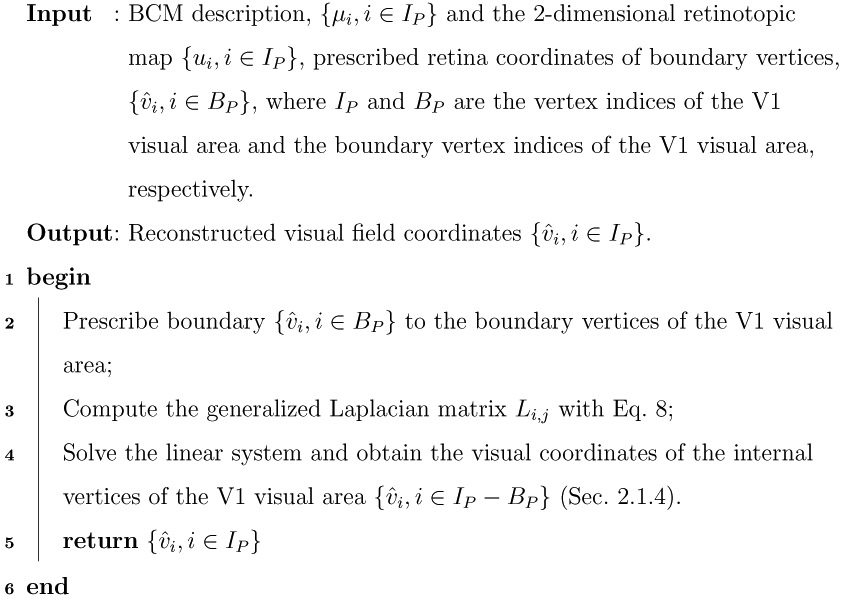
2.5. Smoothing Retinotopic Coordinates

Because of the low signal-to-noise ratio and relatively low spatial resolution of BOLD fMRI, empirical retinotopic maps often do not preserve topology, which is inconsistent with the very notion of the retinotopic map from neurophysiology. Different methods, (e.g., Warnking et al., 2002a; Qiu et al., 2006; Zeidman et al., 2018; Tu et al., 2020b, 2021, In Press), have been proposed to correct or reduce topological violations in fMRI-based retinotopic maps.

In this study, taking advantage of the obtained conformal parameterization of the primary visual area (V1), we smoothed retinotopic maps using thin plate splines (Duchon, 1977) to reduce violations of the topological condition in the retinotopic data. More specifically, we regard the parametric domain D_V1 as the support and fit smooth functions $\widehat{\rho }(u^{(1)},u^{(2)})$ and $\widehat{\theta }(u^{(1)},u^{(2)})$ that best describes the empirical eccentricity and polar angle data sets $\{(u_i^{(1)},u_i^{(2)},{\rho }_i)\}$ and $\{(u_i^{(1)},u_i^{(2)},{\theta }_i)\}$ respectively, where $u_i=(u_i^{(1)},u_i^{(2)})\in D_{V_1}$ is the parametric coordinate, ρ_i and θ_i is the eccentricity and the polar angle for vertex i respectively. To reduce fitting to noise, we only selected points above the 25% pRF model r-square threshold, which is the amount of variance in the time series data explained by the pRF model. Since the spline fitted surface is everywhere continuous and smooth, the smoothed retinotopic maps reduced the number of topology violations on the cortical triangle mesh.

The objective function of the thin plate spline (TPS) is the variational problem,

$$\mathcal{E}=pE(s)+(1-p)S(s).$$ (17)

It consists of a “smoothing” S(s) and “error fitting” E(s) term that are linearly interpolated by adjusting p. The fitting of the thin plate spline to the data is controlled by E(s),

$$E(s)=\sum _i\mid y_j-s(u_i^{(1)},u_i^{(2)}){\mid }^2,$$ (18)

where y_i is the actual data and s(x_i, y_i) is the spline prediction for point j. The smoothness of the spline is controlled by the integrand

$$S(s)=\int \mid {\mathrm{S}}_{xx}{\mid }^2+2\mid {\mathrm{S}}_{xy}{\mid }^2+\mid {\mathrm{S}}_{yy}{\mid }^2,$$ (19)

where S_xx, S_yy, S_xy denote the second partial derivatives of the mapping function s (x_i, y_i). It has been shown in (Wahba, 1990) that the variational problem (Eqn. 17) of minimizing the goodness of fit (Eqn. 18) and smoothness (Eqn. 19) has a unique minimizer s_min.

2.6. Computing the Beltrami Coefficient Maps (BCM)

To compute the BCM, we write the coordinates in complex form, i.e., u = u⁽¹⁾ + iu⁽²⁾ and v = v⁽¹⁾ + iv⁽²⁾ are complex-valued parametric coordinates and visual coordinates, respectively. Thus, the studied retinotopic mapping v = f(u) is a complex to complex map. The visual field coordinate system v = v⁽¹⁾ + iv⁽²⁾ is related to the smoothed eccentricity and polar angle coordinates by $v^{(1)}=\widehat{\rho }\cos (\widehat{\theta })$ and $v^{(2)}=\widehat{\rho }\sin (\widehat{\theta })$.

In the 2-dimensional cortical patch of the V1 visual area $D_{V1}=\{u_i=u_i^{(1)}+u_i^{(2)},i\in I_P\}$ (their associated smoothed visual coordinate $\{v_i=v_i^{(1)}+i{v}_i^{(2)},i\in I_P\}$, where I_P are the vertex indices for the V1 visual area), the retinotopic map function we studied in this work is v_i = f(u_i), i ∈ I_P, as shown in Fig. 7. Because the discrete cortical patch is a triangle mesh, we compute the discrete gradient with Eq. 5 on each face f_i, i ∈ I_F, where I_F are the face index set of the V1 visual area. We obtain the discrete Beltrami coefficient by plugging the discrete gradients into Eq. 2. The result is a set of Beltrami coefficients corresponding to each triangle in D_V1. The Beltrami coefficient at a particular point in D_V1 is linearly interpolated from the adjacent triangles incident to the point.

2.7. Reconstructing the Beltrami Coefficient Maps

Traditional quantitative retinotopic methods (e.g., Balasubramanian et al., 2002; Schira et al., 2007, 2009; Benson et al., 2012, 2014; Benson and Winawer, 2018) adopted a template-based fitting approach, which destroyed the original mapping between the visual cortical surface to the visual field. With the Beltrami coefficients, our quasiconformal Teichmüller theory-based approach provided an opportunity to recover the visual field coordinates from the BCM. It supports the notion that our retinotopic map description is complete.

Specifically, assuming I_P are the vertex indices for the V1 visual area, given the BCM description, [μ_i, i ∈ I_P} and the 2-dimensional retinotopic map {u_i, i ∈ I_P} (Fig. 7 (a)), we can recover the visual coordinates {${\widehat{v}}_i$, i ∈ I_P} (Fig. 7 (c)) using the LBS (Sec. 2.1.4) under suitable normalization. We describe the process in Alg. 3.

2.8. Materials

The retinotopic data used in this work came from the Human Connectome Project (HCP) (Van Essen et al., 2013; Uğurbil et al., 2013). Although the HCP young adults dataset consisted of 1200 observers (https://www.humanconnectome.org/study/hcp-young-adult), only 181 healthy young adults (22-35 years; 109 females, and 72 males) with normal or corrected-to-normal visual acuity participated in the 7T retinotopic map experiments (https://osf.io/bw9ec/wiki/home/). T1-weighted and T2-weighted structural MRI scans at 0.7-mm isotropic resolution were acquired to construct the anatomical brain surface, to which the fMRI retinotopic data were projected. Whole-brain fMRI data at 1.6-mm isotropic resolution and 1-s TR (multiband acceleration 5, in-plane acceleration 2, 85 slices) were collected and processed using the HCP pipelines(Glasser et al., 2013). The data were corrected for head motion and EPI spatial distortion and brought into alignment with the HCP standard surface space. The fMRI data were also denoised for spatially specific structured noise using multirun sICA+FIX (Glasser et al., 2018; Griffanti et al., 2014; Salimi-Khorshidi et al., 2014). The preprocessed data, consisting of 181 subjects 91,282 grayordinates 6 runs 300 time points, are available from ConnectomeDB (https://db.humanconnectome.org/).

Retinotopic mapping stimuli consisted of slowly moving apertures with a dynamic colorful texture placed within them (Benson et al., 2018). Apertures and textures were generated at 768×768 pixels resolution, and constrained to a circular region with a 16.0° diameter. Uniform gray was shown on the display beyond the circular region. One complete experiment consisted of six 300-s runs in which three different types of apertures were presented (wedges, rings, bars). The aperture’s texture was swapped at each aperture update (by randomly selecting from the 100 available texture images without allowing consecutive selections to be the same). Observers were required to attend to a fixation dot and indicate when its color changed. Retinotopic maps were produced by a pRF model called the Compressive Spatial Summation model (Kay et al., 2013b). The model’s predicted fMRI time series is the sum of a stimulus-related time series and a baseline time series. To improve the system robustness, the HCP project fit the pRF model to the data from each of the 181 subjects and three group-average pseudosubjects, which were constructed by averaging time series data across subjects. Each fit produces six quantities of interest, pRF angle, pRF eccentricity, pRF size, pRF gain, percentage of variance explained, and mean signal intensity (Benson et al., 2018). They were used as input to our proposed quantitative characterization framework.

The pRF results and associated stimuli and analysis code adopted in this work are available from (https://osf.io/bw9ec) (Benson et al., 2018) or (https://balsa.wustl.edu/study/show/9Zkk) (Van Essen et al., 2017). We refer the readers to the appendix of the paper (Benson et al., 2018) for the complete processing details and summary statistics. In addition, the preprocessed HCP data and executable code to reproduce all the results presented in this work are available at http://osf.io/5hvg6 (Ta et al., Deposited 10 Jan. 2021).

3. Experimental Results

We processed the retinotopy data from all the 181 healthy observers of the Human Connectome Project (HCP) (Benson et al., 2018) with our proposed processing pipeline. We began with preprocessed HCP retinotopy data, consisting of 3-dimensional cortical surfaces (triangle meshes) with vertex sets that were coregistered with the corresponding retina coordinates (receptive field center), obtained from the best fitting population receptive field (pRF) model (Dumoulin and Wandell, 2008; Kay et al., 2013a; Kriegeskorte et al., 2008; Kay, 2014) of the fMRI time series data. We first unfolded the cortical surface patch onto a 2-dimensional planar disk using the conformal flattening algorithm. In the Cartesian coordinate system, on the disk, (0, 0) corresponds to the foveal confluence, that is, the point at which the horizontal and vertical meridians intersect. We empirically selected a point as the fovea point and move it to (0, 0) with the Möbius transformation to eliminate the conformal ambiguity. We then selected a portion of the V1 retinotopic map for analysis (denoted as D_V1, D_V1 ⊂ D, with ρ : D_V1 → [0°, 8°], θ : D_V1 → [0°, 360°) in our study), using the manually labeled boundaries of V1 on the unit disk that were obtained from the numerically generated template (Glasser et al., 2016) in the HCP preprocessing procedure (Van Essen et al., 2017).

3.1. Conformal Flattening of V1 Retinotopic Map

All 3-dimensional cortical surfaces from 181 observers of the HCP retinotopy data were conformally flattened to the planar disk to allow for the computation of BCM on the 2-dimensional retinotopic map. The quality of the flattening was empirically evaluated with BC at each location on the discrete triangle mesh representation of the flattened cortical surface. The complex norm (magnitude) of BC indicates whether the mapping is conformal. Mathematically, conformal mapping corresponds to smooth complex analytic functions with BC equal to exactly zero. However, because the cortical surface is represented by triangle meshes, the computed complex differentials of the conformal mapping to the planar disk are limited by the quality of the approximating mesh of the original surface and may not be exactly zero. The mean magnitude of BC across all the vertices on the studied V1 area (i,e., D_V1) was 0.0092 ± 0.0009 for the 181 observers in the HCP dataset. The histogram of the BC magnitudes for all 181 observers is shown in (Fig. 8). The near zero BC magnitudes confirmed that the unfolding of the cortical surfaces onto the planar disk were essentially conformal.

Figure 8:

Histogram plot of the Beltrami coefficient (BC). The complex norm (∥μ∥) of the BC in V1 after conformal flattening of 3-dimensional cortical patches to the unit disk. The results were obtained for the 181 HCP observers. The complex norm of the Beltrami coefficient ∥μ∥ in the V1 region were tightly centered around 0. It confirmed that the mapping is conformal.

3.2. Smoothing of V1 Retinotopic Map

We set the parameter p of the error function (Eq. 17) to 0.9 for smoothing the retinotopic maps of all 181 observers in the HCP. This translates to 90% data fitting and 10% smoothness. After we solved Eq. 17 for pRF eccentricity and polar angle data, we obtained smoothed {${\widehat{\rho }}_i$} and {${\widehat{\theta }}_i$}. The obtained smoothed visual field coordinates ($\widehat{\rho }$, $\widehat{\theta }$) reduced the number of topological violations.

Figure 9 (a) shows a typical V1 retinotopic map from the HCP dataset. It contained many violations of the topological condition (Fig. 9 (d)). To illustrate this, we first combined the eccentricity and polar angle maps on the 2-dimensional representation of the cortical surface (Fig. 9 (b)), with the retina coordinates (ρ(D_V1), θ(D_V1))) shown as contour curves. Within the V1 retinotopic map, we selected vertices for which the pRF model could account for at least 25% of variance of the time series data. We referenced them as the high confidence region of the retinotopic map. Directly plotting the visual field coordinates of the retinotopic map (Fig. 9 (c)) revealed 510 flipped triangles (visualized as red triangles in Fig. 9 (d)), indicating that the empirical retinotopic map did not preserve topology in many locations. In fact, there were on average 491±135 flipped triangles (20% to 30%, out of a total of 1987±375 triangles) across the processed retinotopic maps of the 181 observers in the HCP dataset.

Figure 9:

Typical mapping results on V1 retinotopic maps from the HCP. (a-d) Shows the results for a typical retinotopic map without topology correction; (e-h) shows the topology corrected version of the map; (a,e) are the pRF model coregistered retina coordinates on the V1 region located on the disk parameter domain (u⁽¹⁾, u⁽²⁾); (a) shows the color-mapped unsmoothed (ρ, θ) and (e) shows the spline smoothed ($\widehat{\rho }$, $\widehat{\theta }$) retina coordinates; (b,f) are contour curves of coregistered retina coordinates (eccentricity and polar angle lines) overlaid on V1; (b) the original uncorrected coordinates (ρ, θ) and the spline smoothed version ($\widehat{\rho }$, $\widehat{\theta }$); (c,g), are the topology of the retinotopic maps; (c) is for uncorrected polar coordinates (ρ, θ) and (g) is for spline smoothed ($\widehat{\rho }$, $\widehat{\theta }$)). Red colored triangles indicate the triangles that flipped with (d) unsmoothed and (h) spline smoothed retina coordinates.

To reduce violations of the topological condition, we applied a surface spline smoothing algorithm (Duchon, 1977) on the high confidence region of the raw retinotopic map (Figs. 9 (e,f)), which significantly reduced the number of “flipped triangles” (Figs. 9 (g,h)). The corrected map, ($\widehat{\rho }(D_{V1})$, $\widehat{\theta }(D_{V1})$), was smooth and more topology preserving. Across the processed HCP retinotopic maps, surface spline smoothing produced fits with an average r-square of 0.96±0.033 for eccentricity and 0.94±0.030 for polar angle in the high confidence region. It also reduced the average number of flipped triangles from 491 ± 135 to 66 ± 104.

3.3. The Beltrami Coefficient Map

For a continuous surface, the BC is defined for an infinitesimally small circular region on the surface (“local-to-local mapping”). For a discrete surface (e.g., triangle meshes), BC is computed for the smallest discrete unit shape (e.g., triangle face). The BCMs computed from the V1 retinotopic maps of the 181 observers in the HCP dataset were averaged in a common grid space (50 × 50) and visualized as a color map (Fig. 10). The resulting average BCM clearly showed that retinotopic maps are not conformal. Because there was no complete coverage of the visual field by the raw retinotopic maps, we showed three average BCMs in Figs. 10 (a, b, c). In each panel, the average BCM data was shown only when the number of observers with BCM data in the same grid location is greater than the specified ratio of 45/181, 90/181, 145/181. With >= 80% (145/181) of the observers contributing to the average BCM, the “distorted” visual field on the left and right cortical retinotopic maps had BC values of 0.310 ± 0.110 and 0.312 ± 0.105, respectively. The range of the BCMs across individuals suggested that the distortions were similar across observers. On the average BCM, the regions with high average BCMs were located in the fovea region and the boundary of the visual field with high eccentricity (8°). The first (< 1°) was an extremely small cortical area in the foveal region of V1 (densely packed) that could not be resolved with the 7T fMRI measurements (2.0-mm isotropic voxels). The second (> 7°) was located at the upper limit of the eccentricity stimulus (8°) where the voxels contained cortical neurons that were either stimulated or not stimulated by the stimulus (beyond 8°), and the combination might have caused mis-localization (underestimation) of the center of the receptive field in the pRF model.

Figure 10:

The average Beltrami coefficient map (BCM) of the HCP V1 retinotopy data. (a-c) The visual field BCs are sampled across all observers in a common grid space (50×50) and averaged into each grid square. Each grid square is color mapped and visualized when the number of observers with BCM data in that grid is greater than a specified threshold: (a) threshold ≥ 45/181 observers, (b) threshold ≥ 90/181 observers, (c) threshold ≥ 145/181 observers.

The average BCM values became progressively less conformal moving away from the fovea along the vertical meridians; the lower being more non-conformal than the upper vertical meridian. The asymmetry of the BCM and visual performance at different locations on the visual field (Liu et al., 2006) may be linked.

3.4. Reconstructing the Beltrami Coefficient Map

We show the reconstructability of the BCM representation of the V1 retinotopic map from the HCP dataset (Fig. 11) under the condition that V1’s visual coordinates on the boundary are given and the V1 retinotopic map has no flipped triangles (i.e. homeomorphic to the visual field, which satisfies ∣μ∣ < 1). Specifically, we first selected 3 key points on the HCP defined border of V1 (Glasser et al., 2016; Benson et al., 2018), corresponding to (8°, 90°), (8°, 270°), and (0°, 0°) on the visual field. We then divided the vertices on the V1 border between these three points to create 3 continuous segments (the red, green, and blue points in Figs. 11 (b,c)). We solved the LBS for homeomorphic V1 retinotopic maps (n = 139) from the HCP dataset. We found that reconstructed coordinates of the visual field from the BCMs had near-perfect accuracy (error = 1.0e⁻¹⁴) across the entire dataset. Based on these results, we concluded that the BCM characterization of the retinotopic map was complete, that is, it could be used to completely recover the original retinotopic map with fidelity that was only limited by the triangle mesh representation.

Figure 11:

Illustrative example of the reconstruction of the original mapping function from the BCM characterization of empirical retinotopic maps. The retinotopic map is encoded by a unique BCM. Conversely, given a BCM, the associated retinotopic map can be fully reconstructed. (a) Visual field space is depicted with packed circles to illustrate the distortion of the visual field on the retinotopic map; (b) a retinotopic map on the parametric disk domain is quantified by the BCM, which quantifies the vertex-wise shape changes from circles to ellipses; (c) the BCM of the retinotopic map in (b) is used to fully reconstruct the visual field.

4. Discussion

There are three main challenges in retinotopic map research: (1) Because the in vivo retinotopy data suffer from low spatial resolution and low signal-to-noise ratio, the derived retinotopic map often does not satisfy the topological condition. Without addressing this issue, any attempt to quantify the retinotopic map is fundamentally flawed; (2) Although analytical conformal models have been developed to quantify the retinotopic map, there has been no rigorous test of its conformality (Schira et al., 2007). A mathematical framework is necessary to quantify the degree of conformality and model local distortions on the retinotopic map; (3) Existing models of the retinotopic map are not fully reconstructable. That is, it is not possible to accurately project cortical activation onto the visual field. We addressed all these three challenges in this study with a new mathematical framework based on conformal and quasiconformal geometry and successfully applied the framework to analyze a large retinotopy dataset of 181 observers from the HCP.

We first flattened the 3-dimensional cortical surface to a 2-dimensional planar disk with minimal angle distortions using a conformal mapping algorithm. We then projected the V1 retinotopic map onto a unit disk, and used surface spline to reduce violations of the topological condition. Next, we quantified the local distortions of the retinotopic map with the BCM. This allowed us to conclude that the V1 retinotopic map was not conformal but quasiconformal. Finally, we showed that the BCM was fully reconstructable and therefore provided a complete description of the V1 retinotopic map. To our knowledge, it provides the first theoretically rigorous assessment of the conformality with human retinotopic maps.

Our work not only solves the long standing research problem of finding good conformality estimates for the organization of the human primary visual cortex (V1) (Schira et al., 2007) but also achieves a complete description that may help shed new lights in visual neuroscience research or renew discussions on the biological benefits of a particular visual cortex organizational structure. Further, although conformal geometry was frequently adopted in neuroimaging research (e.g., Haker et al., 2000; Hurdal and Stephenson, 2004; Gu et al., 2004; Wang et al., 2007, 2012; Chan et al., 2016; Shi et al., 2017), it was generally used to process structural MRI data. The current work presents our initial efforts to apply conformal geometry to analyze functional MRI data. We hope our research could inspire new ideas and further advance applications of geometry algorithms in medical imaging research.

4.1. Cortical Surface Flattening

Surface parameterizations are traditionally used to enable the the retinotopic map visualization on the flattened cortical representation (e.g., Wandell et al., 2000; Brewer et al., 2005; Wandell et al., 2007). They were also adopted by retinotopic quantification research (e.g., Schwartz, 1980; Balasubramanian et al., 2002; Schira et al., 2007, 2009; Benson et al., 2012, 2014; Benson and Winawer, 2018). Mathematically, it is not possible to preserve both angle and area in cortical flattening because cortical surfaces do not have constant zero Gaussian curvature (i.e., surface geometry is not Euclidean). The following cortical surface flattening methods: (1) multi-dimensional scaling (Schwartz, 1977; Schira et al., 2007, 2009), (2) Tutte planar embedding (Wandell et al., 2000; Floater, 1997; Tutte, 1960), (3) near-isometric flattening (Balasubramanian et al., 2010), and (4) orthogonal projections (of spherically inflated cortical surfaces) or its variants (Benson et al., 2012, 2014; Benson and Winawer, 2018), have been used to study retinotopic maps. However, these methods usually preserve distances and all introduced strong angle distortions, making it impossible to evaluate conformality of the retinotopic map.

Here we took a conformal flattening approach. Therefore, our method can directly evaluate conformality of the retinotopic map. In our prior work (Ta et al., 2014), we flattened the cortical patch using a combination of spherical conformal mapping and stereographic projection. With the same HCP retinotopy data (n=181), the spherical conformal mapping-based flattening results had a mean BC magnitude of 0.0837 ± 0.004, which we improved upon in this work. The minimization of the harmonic energy in the spherical domain (genus-0 surfaces) is a very stable process. However, since it is a global conformal parameterization approach, we cannot identify a specific area (e.g., the visual area V1) to achieve refined conformality. To achieve conformal mapping with best quality in this work, we introduced a new discrete conformal mapping algorithm to flatten the cortical V1 retinotopic patch to the parametric unit disk D. Because D is a conformal map from the 3-dimensional cortical patch, when D is subsequently mapped to another 2-dimensional domain, such as the visual field in the case of the retinotopic map, we can be certain about the Beltrami coefficient results. An alternative is to use least area distortion instead of conformal (angle preserving) cortical flattening (e.g., (Su et al., 2015)) in combination with BC to quantify the retinotopic map (Wang et al., 2019) and to facilitate evaluations of metric properties of the retinotopic map such as cortical magnification factor.

To our knowledge surface conformal parameterization methods have not been frequently adopted in human retinotopic map research. Our hypothesis is that surface conformal parameterization is useful for angle distortion research since retinotopic mapping is considerably angle preserving (Schwartz, 1980; Adams and Horton, 2003). On the other hand, areal preserving approaches may be more appropriate for some area measures, such as cortical magnification factor (CMF) (Daniel and Whitteridge, 1961), in human retinotopic map research. We will explore both surface parameterization schemes in future work.

4.2. Parameter Spaces

Three different parameter spaces were specifically adopted to process retinotopic map data in the current work. (1) Visual field disk space in the pRF model (Dumoulin and Wandell, 2008; Kay et al., 2013b), (2) FreeSurfer’s (Fischl, 2012) spherical parameter space in which the upsampled cortical surfaces was smoothed with SPHARM (Brechbühler et al., 1995; Gu et al., 2004; Chung et al., 2007), and (3) a planar disk domain where the upsampled cortical surface was conformally mapped to and quantification of the retinotopic map is performed. These three parameter spaces were adopted in different stages of the proposed framework and each of them significantly contributed to the feasibility and rigorousness of the proposed framework.

First, the 2D Gaussian kernel was adopted by the pRF model (Dumoulin and Wandell, 2008; Kay et al., 2013b) and its variants (e.g. Merkel et al., 2018, 2020; Lage-Castellanos et al., 2020; Tu et al., 2021, In Press) during preprocessing of retinotopic maps. For each voxel on the cortical surface, the pRF model (Eq. 9) estimates the center (v = (v⁽¹⁾, v⁽²⁾)) and size (σ) of its corresponding receptive field in the visual field space (Fig. 4(“pRF Model Decoding”), Fig. 5(a-d)). The 2D Gaussian kernel (Eq. 11) is typically selected to model the neuronal response around the predicted center in visual field space (planar). The estimated receptive field centers and sizes are then projected onto the cortical surface mesh. Since the pRF model computes the receptive field centers (polar angles and eccentricities) for each voxel on the cortical surface, it is vital to our quantification framework. Second, the mapping from the cortical manifold to the sphere and subsequently to the planar disk were intermediate processing steps in our pipeline (Figs. 4, 6). An important neurophysiological hypothesis we want to evaluate here is whether the human retinotopic map is conformal (i.e., angle preserving). As shown in Fig. 7, we want to evaluate whether f_r is conformal by evaluating whether f = f_r ∘ c⁻¹ is conformal when c is conformal. Clearly, in the discrete case, it is beneficial to compute the conformal mapping, c, as accurately as possible. In finite element analysis, mesh density is an essential metric that is used to control the accuracy of the results. Increasing the density of a mesh will improve the accuracy. Therefore, we applied Loop’s subdivision (Loop, 1987) on the cortical surface and further smoothed the vertex positions of the low resolution cortical surface using SPHARM on its spherical parameterization space. The increased resolution of the anatomical (structural MRI) and functional (fMRI) data improved the precision of our evaluation of retinotopic maps. Compared to the original lower resolution (32K vertices), applying discrete conformal flattening algorithms on the upsampled mesh produced results with better level of conformal accuracy. Finally, the visual cortical surfaces were conformally mapped to the planar domain (disk) to ensure that there is no angle distortion introduced. It benefited our following work which used Beltrami coefficients to quantify the angle distortions and evaluate the conformality of the human retinotopic map. To do that, we first cut out the visual area (including V1 area) and computed a harmonic map to the disk domain. Next, we fine-tuned the conformality by adjusting the Beltrami coefficient on each vertex (Choi and Lui, 2015). Because we mapped the cortical surface to the planar disk with a numerically accurate conformal map, we obtained the most precise quantification of angle distortions of the retinototopic maps. As reported in the manuscript, the mean magnitude of Beltrami coefficients (BC) across all the vertices on the studied V1 area from all 181 HPC observer was 0.0092 ± 0.0009. By comparison, the mean BC magnitude on the same data with our prior disk conformal mapping algorithm (Ta et al., 2014) was 0.0837±0.004. The high numerical accuracy in the anatomical surface conformal mapping allowed us to test the neurophysiological hypothesis more rigorously.

4.3. Topological Condition

As shown in Fig. 9 (d), there were many topological violations in the retinotopic map derived from the BOLD fMRI data. They are not compatible with the very notion of the retinotopic map, which is meant to be topology preserving. We adopted a robust surface spline method to smooth the retinotopic map in the 2-dimensional disk domain, and significantly reduced topological violations. Although we were able to automatically correct the majority of topological errors, we could not completely eliminate them. This is because the parameters of the spline algorithm were selected to not sacrifice fitting accuracy with over smoothing of the data. The method could not correct topological violations in some locations where the amount of noise was too high, often near the fovea or boundaries of the retinotopic map. Although a stronger set of smoothing parameters might eliminate all the topological violations, the quality of the fit to the data would suffer. We tried to achieve a good balance between topological condition and fit quality.

4.4. Conformal vs. Quasiconformal Mapping

Based on the BCMs of the V1 retinotopy map from the 181 observers in the HCP dataset, we concluded that the V1 retinotopic map was not conformal but quasiconformal. One caveat is that the result is based on BOLD fMRI that can only provide a relative low sampling resolution of the retinotopic map, and the magnitudes of the BC may be affected by the sampling density. On the other hand, the spatial resolution of the dataset used in this study is arguably the state of the art, which puts our estimates of the conformality of V1 as the best. Although future studies with more advanced measurement technologies may improve sampling resolution of the retinotopic map and therefore generate improved BC estimates, the mathematical framework developed in the current study would still apply.

The quasiconformality of the retinotopic map, if remains to be true even in future studies with more advanced measurement technologies, could have major implications for our understanding of the visual system. Visual perception and cognition involve a cascade of geometric transformations from the retina to high-level cortical areas. Our perception is mostly veridical and is largely invariant across individuals. If the transformation from the retina to V1 is quasiconformal, e.g., a circle on the retina is mapped onto an ellipse on V1, does it mean that later stages of visual processing can “correct” the distortion? How do visual or neural disorders affect the transformations? Applying the mathematical framework developed in this study to all the visual areas may shed some new light on these questions.

Compared to closed-form quasiconformal parametric models of retinotopic maps (Balasubramanian et al., 2002; Schira et al., 2007), our model does not incorporate assumption of uniformity or symmetry in retinotopic maps. The Beltrami coefficient map that we computed from the HCP dataset exhibited clear differences in angle mapping distortions above and below the horizontal meridian along the vertical meridian whereas the closed-form models are symmetric.

4.5. The Beltrami Coefficient Map

We showed that the original mapping function could be reconstructed from the BCM of V1 under suitable boundary conditions, which can be specified using manual, semi-manual, or numerically computed atlases (Dougherty et al., 2003; Corouge et al., 2004; Das et al., 2009; Wang et al., 2015; Glasser et al., 2016; Benson et al., 2018). Because the geometric transformations of V1 retinotopic maps could be encoded and decoded, we were able to conclude that the BCM provided a complete quantification of the quasiconformal retinotopic map. In fact, it translated the pictorial representation of the retinotopic map into a complete quantitative description, making it possible to apply data analytic tools to characterize retinotopic maps at both individual and population levels. Practically, because we are able reconstruct the original mapping function, we can directly study retinotopic maps in the space of Beltrami coefficients and later reconstruct the mapping functions from maps transformed in that space. For example, our recent work used the BCM to improve topological condition (Tu et al., 2021, In Press) and achieve diffeomorphic registration of retinotopic maps (Tu et al., 2020a). Clinically, due to the reconstructbility, one can derive normative models (Campbell, 2013) of the BCM to study the individual differences in visual perception and visual health. For patients with cortical damage, lesions of the occipital cortex result in areas of cortical blindness affecting the patient’s visual field. Because the original mapping function could be reconstructed from the BCM, we can predict visual field deficits based on their remaining cortical activations and the BCM of the normal population. Rehabilitation or treatment designs could benefit from such accurate localizations of visual field deficits (Sahraie et al., 2006).

4.6. The Jacobian vs. Beltrami Coefficients

Mathematically, the determinant of the Jacobian and Beltrami coefficient are both defined with respect to the tangent space of a surface. Both can be used to determine if a map is orientation preserving. Let the parameterization of the surface be $f:{\mathbb{S}}^2\to {\mathbb{S}}^2$ and the coordinates of the original surface be denoted with x, y and the parameterized surface be denoted with u, v. If f = (u(x, y), v(x, y)) is a smooth diffeomorphism that takes an open boundary surface $S_1\in \mathbb{C}$ to another open boundary surface in $S_2\in \mathbb{C}$ and it has Jacobian determinant J = u_xv_y – v_xu_y > 0, then it is orientation preserving. Similarly, if the Beltrami coefficient modulus ∣μ∣ is less than 1 everywhere on the surface then f is orientation preserving. They are related by the equation, $J=\mid f_z{\mid }^2-\mid f_{\overline{z}}{\mid }^2=\mid f_z{\mid }^2\left(1-\mid \mu {\mid }^2\right)$. Moreover, conformality of a mapping can be determined with the Jacobian or Betrami coefficient. If the Jacobian is the product of a scalar and a rotation matrix or if the Beltrami coefficient μ = 0 then the mapping is conformal.

In medical imaging analysis literature, the surface Jacobian is a widely used quantitative measure in tensor-based morphometry to detect and make inferences about anatomical differences(e.g., Davatzikos, 1996; Thompson et al., 2000; Chung et al., 2007; Wang et al., 2010). It is also widely used to assess the topological condition. We chose the Beltrami coefficient in this study because it is more suitable for retinotopic mapping. First, retinotopic mapping is considerably angle preserving (Schwartz, 1980; Adams and Horton, 2003); with the Beltrami coefficient, we can directly quantify angle distortions. In contrast, the surface Jacobian quantifies area changes, but retinotopic mapping is not area-preserving. Second, as indicated by Theorem 2.1, the Beltrami coefficient map uniquely determines a diffeomorphic mapping between two 2D surfaces, making it possible to reconstruct the mapping if we know the Beltrami coefficients. Therefore, we can achieve a complete description of the human retinotopic map. To our knowledge, there are no efficient and stable methods to utilize surface Jacobian to reconstruct diffeomorphic mappings. In summary, although it may be possible to use surface Jacobian to quantify the diffeomorphic mapping, the Beltrami coefficient is more suitable for modeling retinotopic maps.

4.7. Limitations

It is important to recognize several limitations of the current work. First, although the 7T HCP dataset provided the state-of-the-art data for applying our mathematical framework to characterize the retinotopic map, we are still limited by the low spatial resolution and signal-to-noise ratio in the retinotopy data (Benson et al., 2018). Exploiting other neural activity measures in a multimodal and multi-scale analysis with our mathematical framework may further improve the quantification of the retinotopic map. Second, the surface spline approach smoothed the two dimensions (i.e., ρ and θ) of the visual field independently. It achieved promising results but did not eliminate all topological violations and thus guarantee homeomorphic retinotopic maps. We have developed a topology preserving BCM-based smoothing approach (Tu et al., 2020b) that treats both dimensions simultaneously, producing more promising results. Third, we did not consider the mapping between the retina and the Lateral Geniculate Nucleus (LGN) which was recently shown to constrain direction selectivity in V1 (Nishiyama et al., 2019). Without considering the mapping from the retina to the LGN, and then from the LGN to V1, we cannot localize the origin of the nonconformality in the V1 retinotopic map.

The current study also leads to several exciting new research directions. First, we have only applied our method on V1. A natural extension is to apply it to higher-level retinotopic visual areas such as V2, V3, V4, and IT. This would not only allow us to quantify the retinotopic map in each area but also the geometric transformations between areas in the visual hierarchy. Another extension of the current study is to apply the same framework to the maps in other sensory modalities, such as the tonotopic maps in the auditory system (Barton et al., 2012), the somatosensory maps in the tactile system (Sakai et al., 1995; Gelnar et al., 1998; Chen et al., 2003; Sereno and Huang, 2006), or the motor maps (Meier et al., 2008; Umeda et al., 2019).

5. Conclusion

In this paper, we presented a new mathematical framework based on computational conformal geometry and quasiconformal Teichmüller theory to quantify the retinotopic map. After correcting most of the violations of the topological condition, the method generated an accurate quantitative description of the retinotopic map that was fully reconstructable. The method was successfully applied to a large set of retinotopic maps in V1, and showed that the V1 retinotopic map was quasiconformal. The new framework can be applied to other visual areas and retinotopic maps of individuals with and without eye diseases, and improve our understanding of visual cortical organization in normal and clinical populations.

Highlights.

• A complete and invertible quantitative characterization of human retinotopic maps.

• The framework is based on quasiconformal mapping and theoretically rigorous.

• Smoothing retinotopic maps with thin plate splines to improve topological condition.

• Analysis of HCP retinotopy data (n=181) showed V1 retinotopic map was quasiconformal.

• It can be applied to other visual areas and maps in other sensory areas.

References

- Adams DL, Horton JC, 2003. A precise retinotopic map of primate striate cortex generated from the representation of angioscotomas. Journal of Neuroscience 23, 3771–3789. [DOI] [PMC free article] [PubMed] [Google Scholar]
- Ahlfors L, 1966. Lectures on Quasiconformal Mappings. Mathematical studies, D. Van Nostrand. [Google Scholar]
- Balasubramanian M, Polimeni J, Schwartz EL, 2002. The V1–V2–V3 complex: quasiconformal dipole maps in primate striate and extra-striate cortex. Neural Networks 15, 1157–1163. [DOI] [PubMed] [Google Scholar]
- Balasubramanian M, Polimeni JR, Schwartz EL, 2010. Near-isometric flattening of brain surfaces. Neuroimage 51, 694–703. [DOI] [PMC free article] [PubMed] [Google Scholar]
- Barton B, Venezia JH, Saberi K, Hickok G, Brewer AA, 2012. Orthogonal acoustic dimensions define auditory field maps in human cortex. Proc. Natl. Acad. Sci. U.S.A 109, 20738–20743. [DOI] [PMC free article] [PubMed] [Google Scholar]
- Benson NC, Butt OH, Brainard DH, Aguirre GK, 2014. Correction of distortion in flattened representations of the cortical surface allows prediction of V1-V3 functional organization from anatomy. PLoS Comput. Biol 10, e1003538. [DOI] [PMC free article] [PubMed] [Google Scholar]
- Benson NC, Butt OH, Datta R, Radoeva PD, Brainard DH, Aguirre GK, 2012. The retinotopic organization of striate cortex is well predicted by surface topology. Curr. Biol 22, 2081–2085. [DOI] [PMC free article] [PubMed] [Google Scholar]
- Benson NC, Jamison KW, Arcaro MJ, Vu AT, Glasser MF, Coalson TS, Van Essen DC, Yacoub E, Ugurbil K, Winawer J, Kay K, 2018. The Human Connectome Project 7 Tesla retinotopy dataset: Description and population receptive field analysis. J Vis 18, 23. [DOI] [PMC free article] [PubMed] [Google Scholar]
- Benson NC, Winawer J, 2018. Bayesian analysis of retinotopic maps. Elife 7. [DOI] [PMC free article] [PubMed] [Google Scholar]
- Brechbühler C, Gerig G, Kübler O, 1995. Parametrization of closed surfaces for 3-d shape description. Computer vision and image understanding 61, 154–170. [Google Scholar]
- Brewer AA, Barton B, 2014. Visual cortex in aging and Alzheimer’s disease: changes in visual field maps and population receptive fields. Frontiers in psychology 5. [DOI] [PMC free article] [PubMed] [Google Scholar]
- Brewer AA, Liu J, Wade AR, Wandell BA, 2005. Visual field maps and stimulus selectivity in human ventral occipital cortex. Nature neuroscience 8, 1102. [DOI] [PubMed] [Google Scholar]
- Campbell D, 2013. Normative Data. Springer New York, New York, NY. pp. 2062–2063. [Google Scholar]
- Chan HL, Li H, Lui LM, 2016. Quasi-conformal statistical shape analysis of hippocampal surfaces for alzheimer’s disease analysis. Neurocomput. 175, 177187. [Google Scholar]
- Chen LM, Friedman RM, Roe AW, 2003. Optical imaging of a tactile illusion in area 3b of the primary somatosensory cortex. Science 302, 881–885. [DOI] [PubMed] [Google Scholar]
- Choi PT, Lui LM, 2015. Fast disk conformal parameterization of simply-connected open surfaces. Journal of Scientific Computing 65, 1065–1090. [Google Scholar]
- Chung MK, Dalton KM, Shen L, Evans AC, Davidson RJ, 2007. Weighted fourier series representation and its application to quantifying the amount of gray matter. IEEE Trans Med Imaging 26, 566–581. [DOI] [PubMed] [Google Scholar]
- Corouge I, Dojat M, Barillot C, 2004. Statistical shape modeling of low level visual area borders. Med Image Anal 8, 353–360. [DOI] [PubMed] [Google Scholar]
- Cowey A, 1964. Projection of the retina on to striate and prestriate cortex in the squirrel monkey, saimiri sciureus. Journal of Neurophysiology 27, 366–393. PMID: 14168198. 10.1152/jn.1964.27.3.366. [DOI] [PubMed] [Google Scholar]
- Daniel P, Whitteridge D, 1961. The representation of the visual field on the cerebral cortex in monkeys. The Journal of physiology 159, 203–221. [DOI] [PMC free article] [PubMed] [Google Scholar]
- Das S, Oliver R, Avants B, Radoeva P, Brainard D, Aguirre G, Gee J, 2009. A semi-automated solution for increasing the reliability of manually defined visual area boundaries. Journal of Vision 9, 771–771. [Google Scholar]
- Davatzikos C, 1996. J Comput Assist TomogrSpatial normalization of 3D brain images using deformable models. J Comput Assist Tomogr 20, 656–665. [DOI] [PubMed] [Google Scholar]
- DeYoe EA, Carman GJ, Bandettini P, Glickman S, Wieser J, Cox R, Miller D, Neitz J, 1996. Mapping striate and extrastriate visual areas in human cerebral cortex. Proceedings of the National Academy of Sciences 93, 2382–2386. http://www.pnas.org/content/93/6/2382.full.pdf. [DOI] [PMC free article] [PubMed] [Google Scholar]
- Dougherty RF, Koch VM, Brewer AA, Fischer B, Modersitzki J, Wandell BA, 2003. Visual field representations and locations of visual areas v1/2/3 in human visual cortex. Journal of vision 3, 1–1. [DOI] [PubMed] [Google Scholar]
- Duchon J, 1977. Splines minimizing rotation-invariant semi-norms in sobolev spaces, in: Constructive theory of functions of several variables. Springer, pp. 85–100. [Google Scholar]
- Dumoulin SO, Wandell BA, 2008. Population receptive field estimates in human visual cortex. Neuroimage 39, 647–660. [DOI] [PMC free article] [PubMed] [Google Scholar]
- Engel SA, Glover GH, Wandell BA, 1997. Retinotopic organization in human visual cortex and the spatial precision of functional MRI. Cerebral cortex (New York, NY: 1991) 7, 181–192. [DOI] [PubMed] [Google Scholar]
- Engel SA, Rumelhart DE, Wandell BA, Lee AT, Glover GH, Chichilnisky EJ, Shadlen MN, 1994. fMRI of human visual cortex. Nature 370, 106. [DOI] [PubMed] [Google Scholar]
- Fischl B, 2012. FreeSurfer. Neuroimage 62, 774–781. [DOI] [PMC free article] [PubMed] [Google Scholar]
- Floater MS, 1997. Parametrization and smooth approximation of surface triangulations. Computer Aided Geometric Design 14, 231–250. [Google Scholar]
- Gardiner FP, Lakic N, 2000. Quasiconformal Teichmüller theory. 76, American Mathematical Soc. [Google Scholar]
- Gelnar PA, Krauss BR, Szeverenyi NM, Apkarian AV, 1998. Fingertip representation in the human somatosensory cortex: an fMRI study. Neuroimage 7, 261–283. [DOI] [PubMed] [Google Scholar]
- Glasser MF, Coalson TS, Bijsterbosch JD, Harrison SJ, Harms MP, Anticevic A, Van Essen DC, Smith SM, 2018. Using temporal ICA to selectively remove global noise while preserving global signal in functional MRI data. Neuroimage 181, 692–717. [DOI] [PMC free article] [PubMed] [Google Scholar]
- Glasser MF, Coalson TS, Robinson EC, Hacker CD, Harwell J, Yacoub E, Ugurbil K, Andersson J, Beckmann CF, Jenkinson M, et al. , 2016. A multi-modal parcellation of human cerebral cortex. Nature 536, 171–178. [DOI] [PMC free article] [PubMed] [Google Scholar]
- Glasser MF, Sotiropoulos SN, Wilson JA, Coalson TS, Fischl B, Andersson JL, Xu J, Jbabdi S, Webster M, Polimeni JR, Van Essen DC, Jenkinson M, 2013. The minimal preprocessing pipelines for the Human Connectome Project. Neuroimage 80, 105–124. [DOI] [PMC free article] [PubMed] [Google Scholar]
- Griffanti L, Salimi-Khorshidi G, Beckmann CF, Auerbach EJ, Douaud G, Sexton CE, Zsoldos E, Ebmeier KP, Filippini N, Mackay CE, Moeller S, Xu J, Yacoub E, Baselli G, Ugurbil K, Miller KL, Smith SM, 2014. ICA-based artefact removal and accelerated fMRI acquisition for improved resting state network imaging. Neuroimage 95, 232–247. [DOI] [PMC free article] [PubMed] [Google Scholar]
- Gu X, Wang Y, Chan TF, Thompson PM, Yau ST, 2004. Genus zero surface conformal mapping and its application to brain surface mapping. IEEE Trans Med Imaging 23, 949–958. [DOI] [PubMed] [Google Scholar]
- Haker S, Angenent S, Tannenbaum A, Kikinis R, Sapiro G, Halle M, 2000. Conformal surface parameterization for texture mapping. IEEE Transactions on Visualization and Computer Graphics 6, 181–189. [Google Scholar]
- Hansen KA, David SV, Gallant JL, 2004. Parametric reverse correlation reveals spatial linearity of retinotopic human V1 BOLD response. Neuroimage 23, 233–241. [DOI] [PubMed] [Google Scholar]
- Ho-Phuoc T, Guerin-Dugue A, 2009. A new self-organizing map for dissimilarity data. Encyclopedia of Artificial Intelligence , 1244–1252. [Google Scholar]
- Horton JC, Hoyt WF, 1991. The representation of the visual field in human striate cortex: a revision of the classic holmes map. Archives of ophthalmology 109, 816–824. [DOI] [PubMed] [Google Scholar]
- Hubel DH, Wiesel TN, 1965. Receptive fields and functional architecture in two nonstraiate visual areas (18 and 19) of the cat. J. Neurophysiol 28, 229–289. [DOI] [PubMed] [Google Scholar]
- Hurdal MK, Stephenson K, 2004. Cortical cartography using the discrete conformal approach of circle packings. Neuroimage 23 Suppl 1, S119–128. [DOI] [PubMed] [Google Scholar]
- Jin M, Gu X, He Y, Wang Y, 2018. Conformal Geometry: Computational Algorithms and Engineering Applications. Springer. [Google Scholar]
- Kammen A, Law M, Tjan BS, Toga AW, Shi Y, 2016. Automated retinofugal visual pathway reconstruction with multi-shell HARDI and FOD-based analysis. Neuroimage 125, 767–779. [DOI] [PMC free article] [PubMed] [Google Scholar]
- Kay K, 2014. analyzeprf: stimuli and code for pRF analysis. http://cvnlab.net/analyzePRF/. Accessed: 2019-08-13. [Google Scholar]
- Kay KN, Winawer J, Mezer A, Wandell BA, 2013a. Compressive spatial summation in human visual cortex. J. Neurophysiol 110, 481–494. [DOI] [PMC free article] [PubMed] [Google Scholar]
- Kay KN, Winawer J, Mezer A, Wandell BA, 2013b. J NeurophysiolCompressive spatial summation in human visual cortex. J Neurophysiol 110, 481–494. [DOI] [PMC free article] [PubMed] [Google Scholar]
- Kriegeskorte N, Mur M, Ruff DA, Kiani R, Bodurka J, Esteky H, Tanaka K, Bandettini PA, 2008. Matching categorical object representations in inferior temporal cortex of man and monkey. Neuron 60, 1126–1141. [DOI] [PMC free article] [PubMed] [Google Scholar]
- Lage-Castellanos A, Valente G, Senden M, De Martino F, 2020. Front Neurosci-Investigating the Reliability of Population Receptive Field Size Estimates Using fMRI. Front Neurosci 14, 825. [DOI] [PMC free article] [PubMed] [Google Scholar]
- Liu T, Heeger DJ, Carrasco M, 2006. Neural correlates of the visual vertical meridian asymmetry. Journal of Vision 6, 12–12. [DOI] [PMC free article] [PubMed] [Google Scholar]
- Loop C, 1987. Smooth subdivision surfaces based on triangles. Master’s Thesis, University of Utah, Department of Mathematics; . [Google Scholar]
- Lui L, Lam K, Wong T, Gu X, 2013. Texture map and video compression using Beltrami representation. SIAM Journal on Imaging Sciences 6, 1880–1902. 10.1137/120866129. [DOI] [Google Scholar]
- Lui LM, Wong TW, Zeng W, Gu X, Thompson PM, Chan TF, Yau ST, 2012. Optimization of surface registrations using beltrami holomorphic flow. Journal of scientific computing 50, 557–585. [Google Scholar]
- Meier JD, Aflalo TN, Kastner S, Graziano MS, 2008. Complex organization of human primary motor cortex: a high-resolution fMRI study. Journal of neurophysiology 100, 1800–1812. [DOI] [PMC free article] [PubMed] [Google Scholar]
- Merkel C, Hopf JM, Schoenfeld MA, 2018. Hum Brain MappSpatial elongation of population receptive field profiles revealed by model-free fMRI back-projection. Hum Brain Mapp 39, 2472–2481. [DOI] [PMC free article] [PubMed] [Google Scholar]
- Merkel C, Hopf JM, Schoenfeld MA, 2020. Hum Brain MappModulating the global orientation bias of the visual system changes population receptive field elongations. Hum Brain Mapp 41, 1765–1774. [DOI] [PMC free article] [PubMed] [Google Scholar]
- Meyer M, Desbrun M, Schröder P, Barr AH, 2003. Discrete differential-geometry operators for triangulated 2-manifolds, in: Hege HC, Polthier K (Eds.), Visualization and Mathematics III, Springer Berlin Heidelberg, Berlin, Heidelberg. pp. 35–57. [Google Scholar]
- Michel MM, Chen Y, Geisler WS, Seidemann E, 2013. An illusion predicted by V1 population activity implicates cortical topography in shape perception. Nature neuroscience 16, 1477–1483. [DOI] [PMC free article] [PubMed] [Google Scholar]
- Morland AB, Baseler HA, Hoffmann MB, Sharpe LT, Wandell BA, 2001. Abnormal retinotopic representations in human visual cortex revealed by fMRI. Acta Psychol (Amst) 107, 229–247. [DOI] [PubMed] [Google Scholar]
- Nishiyama M, Matsui T, Murakami T, Hagihara KM, Ohki K, 2019. Cell-type-specific thalamocortical inputs constrain direction map formation in visual cortex. Cell Reports 26, 1082–1088. [DOI] [PubMed] [Google Scholar]
- Qiu A, Rosenau BJ, Greenberg AS, Hurdal MK, Barta P, Yantis S, Miller MI, 2006. Estimating linear cortical magnification in human primary visual cortex via dynamic programming. Neuroimage 31, 125–138. [DOI] [PubMed] [Google Scholar]
- Sahraie A, Trevethan CT, MacLeod MJ, Murray AD, Olson JA, Weiskrantz L; 2006. Increased sensitivity after repeated stimulation of residual spatial channels in blindsight. Proc. Natl. Acad. Sci. U.S.A 103, 14971–14976. [DOI] [PMC free article] [PubMed] [Google Scholar]
- Sakai K, Watanabe E, Onodera Y, Itagaki H, Yamamoto E, Koizumi H, Miyashita Y, 1995. Functional mapping of the human somatosensory cortex with echo-planar MRI. Magnetic resonance in medicine 33, 736–743. [DOI] [PubMed] [Google Scholar]
- Salimi-Khorshidi G, Douaud G, Beckmann CF, Glasser MF, Griffanti L, Smith SM, 2014. Automatic denoising of functional MRI data: combining independent component analysis and hierarchical fusion of classifiers. Neuroimage 90, 449–468. [DOI] [PMC free article] [PubMed] [Google Scholar]
- Schira MM, Tyler CW, Breakspear M, Spehar B, 2009. The foveal confluence in human visual cortex. Journal of Neuroscience 29, 9050–9058. [DOI] [PMC free article] [PubMed] [Google Scholar]
- Schira MM, Wade AR, Tyler CW, 2007. Two-dimensional mapping of the central and parafoveal visual field to human visual cortex. Journal of neurophysiology 97, 4284–4295. [DOI] [PubMed] [Google Scholar]
- Schneider W, Noll DC, Cohen JD, 1993. Functional topographic mapping of the cortical ribbon in human vision with conventional MRI scanners. Nature 365, 150. [DOI] [PubMed] [Google Scholar]
- Schwartz E, 1985. On the mathematical structure of the retinotopic mapping of primate striate cortex. Science 227, 1066. [DOI] [PubMed] [Google Scholar]
- Schwartz EL, 1977. Spatial mapping in the primate sensory projection: analytic structure and relevance to perception. Biological cybernetics 25, 181–194. [DOI] [PubMed] [Google Scholar]
- Schwartz EL, 1980. Computational anatomy and functional architecture of striate cortex: a spatial mapping approach to perceptual coding. Vision research 20, 645–669. [DOI] [PubMed] [Google Scholar]
- Schwarzkopf DS, Song C, Rees G, 2011. The surface area of human V1 predicts the subjective experience of object size. Nature neuroscience 14, 28–30. [DOI] [PMC free article] [PubMed] [Google Scholar]
- Sereno MI, Dale AM, Reppas JB, Kwong KK, Belliveau JW, Brady TJ, Rosen BR, Tootell RB, 1995. Borders of multiple visual areas in humans revealed by functional magnetic resonance imaging. Science 268, 889–893. [DOI] [PubMed] [Google Scholar]
- Sereno MI, Huang RS, 2006. A human parietal face area contains aligned head-centered visual and tactile maps. Nature neuroscience 9, 1337–1343. [DOI] [PubMed] [Google Scholar]
- Sethian J, 1999. Level Set Methods and Fast Marching Methods: Evolving Interfaces in Computational Geometry, Fluid Mechanics, Computer Vision, and Materials Science. Cambridge Monographs on Applied and Computational Mathematics, Cambridge University Press. [Google Scholar]
- Shi J, Zhang W, Tang M, Caselli RJ, Wang Y, 2017. Conformal invariants for multiply connected surfaces: Application to landmark curve-based brain morphometry analysis. Med Image Anal 35, 517–529. [DOI] [PMC free article] [PubMed] [Google Scholar]
- Styner M, Oguz I, Xu S, Brechbhler C, Pantazis D, Levitt JJ, Shenton ME, Gerig G, 2006. Framework for the Statistical Shape Analysis of Brain Structures using SPHARM-PDM. Insight J , 242–250. [PMC free article] [PubMed] [Google Scholar]
- Su Z, Wang Y, Shi R, Zeng W, Sun J, Luo F, Gu X, 2015. Optimal mass transport for shape matching and comparison. IEEE Trans Pattern Anal Mach Intell 37, 2246–2259. [DOI] [PMC free article] [PubMed] [Google Scholar]
- Swindale NV, Shoham D, Grinvald A, Bonhoeffer T, Hbener M, 2000. Nat NeurosciVisual cortex maps are optimized for uniform coverage. Nat Neurosci 3, 822–826. [DOI] [PubMed] [Google Scholar]
- Ta D, Shi J, Barton B, Brewer A, Lu ZL, Wang Y, 2014. Characterizing human retinotopic mapping with conformal geometry: a preliminary study, in: Medical Imaging 2014: Image Processing, International Society for Optics and Photonics. p. 90342A. [Google Scholar]
- Ta D, Tu Y, Lu ZL, Wang Y, Deposited 10 January. 2021. Quantitative characterization of the human retinotopic map based on quasiconformal mapping. http://osf.io/5hvg6. [DOI] [PMC free article] [PubMed] [Google Scholar]
- Talbot S, Marshall W, 1941. Physiological studies on neural mechanisms of visual localization and discrimination. American Journal of Ophthalmology 24, 1255–1264. [Google Scholar]
- Thompson JM, Woolsey CN, Talbot SA, 1950. Visual areas I and II of cerebral cortex of rabbit. J. Neurophysiol. 13, 277–288. [DOI] [PubMed] [Google Scholar]
- Thompson PM, Giedd JN, Woods RP, MacDonald D, Evans AC, Toga AW, 2000. NatureGrowth patterns in the developing brain detected by using continuum mechanical tensor maps. Nature 404, 190–193. [DOI] [PubMed] [Google Scholar]
- Tootell R, 1985. Deoxyglucose, retinotopic mapping and the complex log model in striate cortex. Science 227, 1066.17794232 [Google Scholar]
- Tootell RB, Hadjikhani NK, Vanduffel W, Liu AK, Mendola JD, Sereno MI, Dale AM, 1998. Functional analysis of primary visual cortex (V1) in humans. Proceedings of the National Academy of Sciences 95, 811–817. [DOI] [PMC free article] [PubMed] [Google Scholar]
- Tootell RB, Reppas JB, Kwong KK, Malach R, Born RT, Brady TJ, Rosen BR, Belliveau JW, 1995. Functional analysis of human MT and related visual cortical areas using magnetic resonance imaging. Journal of Neuroscience 15, 3215–3230. [DOI] [PMC free article] [PubMed] [Google Scholar]
- Tu Y, Ta D, David Gu X, Lu ZL, Wang Y, 2020a. Diffeomorphic registration for retinotopic mapping via quasiconformal mapping, in: 2020 IEEE 17th International Symposium on Biomedical Imaging (ISBI), pp. 687–691. [DOI] [PMC free article] [PubMed] [Google Scholar]
- Tu Y, Ta D, Lu ZL, Wang Y, 2020b. Diffeomorphic smoothing for retinotopic mapping. Proc IEEE Int Symp Biomed Imaging 2020, 534–538. [DOI] [PMC free article] [PubMed] [Google Scholar]
- Tu Y, Ta D, Lu ZL, Wang Y, 2021, In Press. Topology-preserving smoothing of retinotopic maps. PLoS Comput. Biol . [DOI] [PMC free article] [PubMed] [Google Scholar]
- Tusa R, Palmer L, Rosenquist A, 1978. The retinotopic organization of area 17 (striate cortex) in the cat. Journal of Comparative Neurology 177, 213–235. [DOI] [PubMed] [Google Scholar]
- Tutte WT, 1960. Convex representations of graphs. Proceedings of the London Mathematical Society s3-10, 304–320. https://londmathsoc.onlinelibrary.wiley.com/doi/pdf/10.1112/plms/s3-10.1.304. [Google Scholar]
- Uğurbil K, Xu J, Auerbach EJ, Moeller S, Vu AT, Duarte-Carvajalino JM, Lenglet C, Wu X, Schmitter S, Van de Moortele PF, et al. , 2013. Pushing spatial and temporal resolution for functional and diffusion MRI in the human connectome project. Neuroimage 80, 80–104. [DOI] [PMC free article] [PubMed] [Google Scholar]
- Umeda T, Isa T, Nishimura Y, 2019. The somatosensory cortex receives information about motor output. Science advances 5, eaaw5388. [DOI] [PMC free article] [PubMed] [Google Scholar]
- Van Essen DC, Newsome WT, Maunsell JH, 1984. The visual field representation in striate cortex of the macaque monkey: asymmetries, anisotropies, and individual variability. Vision research 24, 429–448. [DOI] [PubMed] [Google Scholar]
- Van Essen DC, Smith J, Glasser MF, Elam J, Donahue CJ, Dierker DL, Reid EK, Coalson T, Harwell J, 2017. The brain analysis library of spatial maps and atlases (balsa) database. Neuroimage 144, 270–274. [DOI] [PMC free article] [PubMed] [Google Scholar]
- Van Essen DC, Smith SM, Barch DM, Behrens TE, Yacoub E, Ugurbil K, Consortium WMH, et al. , 2013. The WU-Minn human connectome project: an overview. Neuroimage 80, 62–79. [DOI] [PMC free article] [PubMed] [Google Scholar]
- Vilenkin N, 1968. Special Functions and the Theory of Group Representations. American Mathematical Society, Providence. [Google Scholar]
- Wahba G, 1990. Spline models for observational data. SIAM. [Google Scholar]
- Wandell BA, Chial S, Backus BT, 2000. J Cogn NeurosciVisualization and measurement of the cortical surface. J Cogn Neurosci 12, 739–752. [DOI] [PubMed] [Google Scholar]
- Wandell BA, Dumoulin SO, Brewer AA, 2007. NeuronVisual field maps in human cortex. Neuron 56, 366–383. [DOI] [PubMed] [Google Scholar]
- Wandell BA, Winawer J, 2011. Imaging retinotopic maps in the human brain. Vision research 51, 718–737. [DOI] [PMC free article] [PubMed] [Google Scholar]
- Wang L, Mruczek RE, Arcaro MJ, Kastner S, 2015. Probabilistic maps of visual topography in human cortex. Cereb. Cortex 25, 3911–3931. [DOI] [PMC free article] [PubMed] [Google Scholar]
- Wang Q, Burkhalter A, 2007. Area map of mouse visual cortex. J. Comp. Neurol 502, 339–357. [DOI] [PubMed] [Google Scholar]
- Wang Y, Lui LM, Gu X, Hayashi KM, Chan TF, Toga AW, Thompson PM, Yau ST, 2007. Brain surface conformal parameterization using Riemann surface structure. IEEE Trans Med Imaging 26, 853–865. [DOI] [PMC free article] [PubMed] [Google Scholar]
- Wang Y, Shi J, Yin X, Gu X, Chan TF, Yau ST, Toga AW, Thompson PM, 2012. Brain surface conformal parameterization with the Ricci flow. IEEE Trans Med Imaging 31, 251–264. [DOI] [PMC free article] [PubMed] [Google Scholar]
- Wang Y, Ta D, Lu ZL, 2019. Apparatus and method for quantification of the mapping of sensory areas of the brain. US Patent Application number: 16230284.
- Wang Y, Zhang J, Gutman B, Chan TF, Becker JT, Aizenstein HJ, Lopez OL, Tamburo RJ, Toga AW, Thompson PM, 2010. NeuroimageMultivariate tensor-based morphometry on surfaces: application to mapping ventricular abnormalities in HIV/AIDS. Neuroimage 49, 2141–2157. [DOI] [PMC free article] [PubMed] [Google Scholar]
- Warnking J, Dojat M, Guérin-Dugué A, Delon-Martin C, Olympieff S, Richard N, Chéhikian A, Segebarth C, 2002a. fMRI retinotopic mappingstep by step. NeuroImage 17, 1665–1683. [DOI] [PubMed] [Google Scholar]
- Warnking J, Dojat M, Gurin-Dugu A, Delon-Martin C, Olympieff S, Richard N, Chhikian A, Segebarth C, 2002b. NeuroimagefMRI retinotopic mapping–step by step. Neuroimage 17, 1665–1683. [DOI] [PubMed] [Google Scholar]
- Yu X, Lei N, Wang Y, Gu X, 2017. Intrinsic 3D Dynamic Surface Tracking based on Dynamic Ricci Flow and Teichmuller Map. Proc IEEE Int Conf Comput Vis 2017, 5400–5408. [DOI] [PMC free article] [PubMed] [Google Scholar]
- Zeidman P, Silson EH, Schwarzkopf DS, Baker CI, Penny W, 2018. Bayesian population receptive field modelling. Neuroimage 180, 173–187. [DOI] [PMC free article] [PubMed] [Google Scholar]
- Zeng W, Lui LM, Luo F, Chan TFC, Yau ST, Gu DX, 2012. Computing quasiconformal maps using an auxiliary metric and discrete curvature flow. Numerische Mathematik 121, 671–703. [Google Scholar]
- Zhang W, Mi L, Thompson PM, Wang Y, 2019. A Geometric Framework for Feature Mappings in Multimodal Fusion of Brain Image Data. Inf Process Med Imaging 11492, 617–630. [DOI] [PMC free article] [PubMed] [Google Scholar]