Abstract
Purpose
Low‐signal correction (LSC) in the raw counts domain has been shown to effectively reduce noise streaks in CT because the data inconsistency associated with photon‐starved regions may be mitigated prior to the log transformation step. However, a systematic study of the performance of these raw data correction methods is still missing in literature. The purpose of this work was to provide such a systematic study for two well‐known low‐signal correction schemes using either the adaptive trimmed mean (ATM) filter or the anisotropic diffusion (AD) filter in the raw counts domain.
Methods
Image data were acquired experimentally using an anthropomorphic chest phantom and a benchtop cone‐beam CT (CBCT) imaging system. Phantom scans were repeated 50 times at a reduced dose level of 0.5 mGy and a reference level of 1.9 mGy. The measured raw counts at 0.5 mGy underwent LSC using the ATM and AD filters. Two relevant parameters were identified for each filter and approximately one hundred operating points in each parameter space were analyzed. Following LSC and log transformation, FDK reconstruction was performed for each case. Noise and spatial resolution properties were assessed across the parameter spaces that define each LSC filter; the results were summarized through 2D contour maps to better understand the trade‐offs between these competing image quality features. 2D noise power spectrum (NPS) and modulation transfer function (MTF) were measured locally at two spatial locations in the field‐of‐view (FOV): a posterior region contaminated by noise streaks and an anterior region away from noise streaks. An isotropy score metric was introduced to characterize the directional dependence of the NPS and MTF (viz., ϵ NPS and ϵ MTF , respectively), with a range from 0 for highly anisotropic to 1 for perfectly isotropic. The noise magnitude and coarseness were also measured.
Results
(a) Both the ATM and AD LSC methods were successful in reducing noise streaks, but their noise and spatial resolution properties were found to be highly anisotropic and shift‐variant. (b) NPS isotropy scores in the posterior region were generally improved from ϵ NPS = 0.09 for the images without LSC to the range ϵ NPS = (0.11, 0.67) for ATM and ϵ NPS = (0.06, 0.67) for AD, depending on the filter parameters used. (c) The noise magnitude was reduced across the parameter space of either LSC filter whenever a change along the axis of the controlling parameter led to stronger raw data filtration. Changes in noise magnitude were inversely related to changes in spatial resolution along the direction perpendicular to the streaks. No correlation was found, however, between the contour maps of noise magnitude and the NPS isotropy. (d) Both filters influenced the noise coarseness anisotropically, with coarser noise occurring along directions perpendicular to the noise streaks. The anisotropic noise coarseness was intrinsically and directly related to resolution losses in a given direction: coarseness plots mimic the topography of the 2D MTF, i.e., the coarser the noise, the lower the resolution.
Conclusions
Both AD and ATM LSC schemes enable low‐dose CBCT imaging. However, it was found that noise magnitude and overall spatial resolution vary considerably across the parameter space for each filter, and more importantly these image quality features are highly anisotropic and shift‐variant.
Keywords: adaptive trimmed mean filter, anisotropic diffusion, CT, low‐signal correction, noise streaks, spatial resolution
1. Introduction
Ionizing radiation used in x‐ray computed tomography (CT) remains a public concern because of the associated small but non‐zero potential cancer risk.1 Much effort has therefore been spent developing innovative CT technologies involving both software and hardware and optimizing scanning protocols to acquire CT images at a reduced dose with acceptable image quality. One approach to reduce radiation dose in CT is decreasing the incident photon fluence; however, a reduced number of photons at the detector leads to a marked increase in the measured fluctuations of detected photons. These large uncertainties are subsequently amplified by the log transformation to generate line integral projection data.2 As a result, two potential consequences may arise with the reduction of photon fluence: an increase in noise magnitude and an increased likelihood for structured noise streaks to appear in the reconstructed image. Therefore, it is critically important to handle the photon‐starved projection measurements such that the associated data inconsistency can be reduced and the presence of noise streaks in the final CT image can be effectively mitigated.
To address these challenges in low‐dose CT, three major classes of denoising schemes have been proposed to accompany the conventional image reconstruction pipeline, viz. filtered backprojection (FBP): (a) denoising in the image domain after image reconstruction;3, 4, 5 (b) sinogram smoothing techniques, i.e., denoising line integral data in the log‐transformed projection data domain;6, 7, 8, 9 and (c) low‐signal correction (LSC) schemes2, 10 performed directly in the raw counts domain before the log transformation step is taken.
Despite the partial success of schemes (a) and (b) for noise magnitude reduction, schemes that work directly in the raw counts domain (c) are in principle, more effective at reducing noise streaks caused by photon starvation, since once the log transformation step is performed, the signal variance may be amplified to a degree that is hard to recover from later on in the data processing chain. A widely used LSC method is the adaptive trimmed mean (ATM) filter.2 An alternative denoising method that has shown good performance in low‐dose CT is anisotropic diffusion11 (AD). However, AD has only been implemented in the log‐transformed domain,12 and it therefore remains to be investigated whether or not AD has additional potential in the raw counts domain. The main advantage of AD is that it can guide the denoising process by extracting the image object edge structural information, potentially favoring spatial resolution and the conspicuity of low contrast features. Both the ATM and AD methods, as well as a conventional boxcar filter for comparison purposes, were investigated in this paper to study the impact of their key parameters on the filter performance.
In order to properly account for the potential nonlinear behavior and to optimize filter parameter selection, an appropriate imaging performance assessment framework is needed. Current approaches to evaluate the imaging performance of a given filtration method and to optimize parameter selection have been limited to a subjective assessment of noise streaks removal and structural preservation in the difference images2, 6 between the reference and the denoised images, or quantitative measures of noise magnitude and spatial resolution. However, there are two major limitations in these analyses: (a) To produce datasets for noise and spatial resolution measurements, either numerical phantoms with a noise model were used or simulated noise and objects were inserted in real data from a single scan.2, 6, 8, 9, 10 Since it is difficult to know the noise distributions from actual experimental systems or to model the many factors affecting spatial resolution, measurements will highly depend on choices made during simulation. (b) Only zero‐dimensional (0D) or one‐dimensional (1D) surrogates of noise and spatial resolution have been considered in most cases;2, 4, 5, 6, 8, 9, 10 the noise magnitude lacks frequency information, and although the directional dependence of spatial resolution has typically been described qualitatively, the resolution metrics that have been used — edge profile gradients, point spread function (PSF) widths, or 1D modulation transfer functions (MTF) — do not quantify the potential directional dependence comprehensively. In order to obtain a deeper understanding of these important image quality features, higher dimensional analysis of the frequency distribution of noise and the response of the CT imaging system to multiple frequencies is needed, and the directional dependence needs to be characterized.
The purpose of this work was to provide a systematic study for ATM and AD based LSC schemes in the raw counts domain. This work is divided in two parts: Part I describes in detail the implementation of both LSC methods and the assessment of their spatial resolution and noise performances. More specifically in Part I, ATM and AD were parameterized and used to filter raw data from a physical anthropomorphic phantom scanned on a CBCT system under a severe photon starvation scenario. An exhaustive exploration of the filter parameter space was performed, and an ensemble averaging approach13, 14 was taken to study the noise and spatial resolution properties of each LSC method across its parameter space. The local two‐dimensional (2D) modulation transfer function (MTF) and the 2D noise power spectrum (NPS) were measured, and noise magnitude and texture as well as spatial resolution directionality were assessed across the parameter space. These frequency‐dependent metrics provide a comprehensive understanding of noise and spatial resolution as it depends on the spatial location and filter parameters. Part II15 of this work will then incorporate these frequency dependent metrics into a task‐based detectability framework to optimize parameter selection for a given LSC method.
2. Materials and methods
2.A. Low‐signal correction methods
In this work, the measured counts at a given view angle θ and detector spatial location (u, v) are denoted as , where i is the index of the detector pixel located at (u, v). Using this notation, three LSC schemes — a conventional linear boxcar filter, the adaptive trimmed mean filter, and the anisotropic diffusion filter — are presented in the following subsections.
2.A.1. Mean boxcar filter
The simplest LSC scheme is a shift‐invariant linear filter for the raw data. For this work, mean filtering with a 2D boxcar function was chosen. The 2D boxcar can be defined as a square with side length s (units of pixels) and density 1/s2 inside the square and 0 outside. Convolution of the raw data in each view angle with this function yields the LSC data. For brevity, this method will be referred to as “BOX”.
2.A.2. Adaptive trimmed mean filter
The ATM16 is an Order Statistical (OS) filtration method that forms the basis of some current state‐of‐the‐art LSC schemes in clinical CT.2 As will be described in more detail below, “trimmed” refers to how many of the sorted values to exclude from the averaging step; and “adaptive” refers to the functional dependence of two items, (a) the size of the window used for sorting, and (b) the proportion of this sorted window to trim away.
The adaptive mean (AM) filter is a mean filter with adjustable window width, namely, for a given signal at location centered at detector spatial location (u, v), the filtered value is equal to the average of all signal values in a specific neighborhood of that location, e.g., a centered window with dimension W × W, where the extent of the window W depends on the original signal level itself. Specifically, a window width W can be calculated as a function of P θ (u, v) and the filtered value P θ,f (u, v) is equal to the mean signal level of P θ in a W × W window centered at (u, v). The window width function is defined piecewisely as
| (1) |
Note that W has units of pixels, and the range is all real numbers ∈[1, W 0], regardless of whether the input signal P θ is continuous or sampled. If the sampling interval on the detector is ∆u having units of length, then the real window width is simply W ∆u. Figure 1 displays examples of various window width functions overlaid the histogram of raw count data P θ in a given view.
Figure 1.
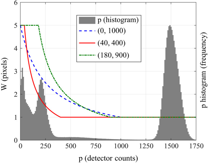
Example of a histogram of the raw count data in a given view overlaid with the signal‐dependent window function W (p) parameterized by W 0 = 5 and various (p l , p h ) pairs. [Color figure can be viewed at wileyonlinelibrary.com]
The window width function is designed so that the largest window width W 0 is used to filter signals whose levels are below a low threshold p l , where the signal‐to‐noise ratio (SNR) is poor and electronic noise may have a non‐negligible impact. In contrast, for signals with levels exceeding a high threshold p h (p h ≥ p l) , where the SNR is very high, the mean is performed over a window that is only 1 pixel wide, i.e., the signal is not filtered. For signals with levels somewhere in the middle of these two thresholds, the window width is formulated as being inversely proportional to the signal level so as to make W (p) a piecewise continuous function.
To facilitate the numerical implementation of the AM filter for the digital image P θ , the adaptive window width in Eq. (1) is mapped to integer values as follows:
| (2) |
where gives the largest integer less than or equal to w. Namely, an adaptive window width in Eq. (1) is mapped to the smallest odd integer greater than or equal to W.
To facilitate the following discussion, let ρ represent a column vector of length M containing only the signal values from this 2D window, i.e., and it's (interpolated) neighbors included by Eqs. (1) and (2). The AM filter is thus
| (3) |
where 1 T is the transpose of an all ones column vector of length M.
ATM filtration is done by adding signal trimming to the above AM filtration procedure such that one can threshold out both very high and very low signal values. This can be accomplished by sorting signal values ρ from high to low to generate a new sequence of signals denoted as . After this sorting step, the average is then taken among the central values only. As a result, the AM mean filter in Eq. (3) is changed into the desired ATM filter as follows:
| (4) |
where elements of the ξ column vector are given by
| (5) |
where gives the smallest integer greater than or equal to w. The trimming proportion α can also be signal dependent. In this work, it was allowed to linearly climb from 0 at the low signal threshold to 0.5 for the high threshold:
| (6) |
The motivation for this choice was to have the regions of low SNR be filtered with the standard mean filter (α = 0 case) and to have regions with high SNR signals be filtered with a median filter (α → 0.5 case). Cases where M(1 − 2α) < 1 were flagged for median filtration so that Eq. (5) was well‐defined.
2.A.3. Anisotropic diffusion filter
Without invoking the use of order statistics, one can also perform edge preserving spatial filtration in the raw counts domain to handle the photon starvation problem. In this regard, AD,11, 17, 18, 19, 20, 21 a partial differential equation (PDE)‐based iterative image processing method, is a good choice.
Increasing the number of iterations in the AD algorithm is analogous to moving forward in time for the diffusion process. One important feature of AD is that it enables a spatially variant filtration of an image through the use of a brightness gradient function. Preferably, this spatially variant filtration would give preference to intraregion smoothing rather than inter‐region smoothing, so that after each iteration of AD the result is a version of the input signal with reduced noise and without the associated loss of relevant structural information.
By introducing a pseudo‐time dimension, τ, where signal can be allowed to diffuse, the continuous anisotropic diffusion equation for the 2D detector signal in view angle θ is
| (7) |
where D θ is the diffusion coefficient which depends on both the spatial location and the pseudo‐time τ, and the symbols div, ∇, and ∇2 correspond to the divergence, gradient, and Laplacian operators, respectively.
It can be shown that if D is a function of ∇ P, then both terms in Eq. (7) have similar polarity, with the Laplacian term having a smaller magnitude than the dot product term. Here, similar polarity means that the signals are strongly correlated with each other. Therefore, in a digital implementation, the potentially costly and numerically unstable second‐order term does not need to be explicitly calculated. The pseudo‐time‐derivative and dot product term can thus be discretized as follows11
| (8) |
| (9) |
where ∆τ is the step size. In this digital representation, t is now the index of the iteration number. The dot product term was written as the summation over components extended to B‐nearest neighbors and ∇ b denotes the directional derivative along the b‐th direction. In this work, B = 8 and ∆τ = 1/8.
The digital form to map the raw data gradient to a diffusion coefficient for a given direction b is
| (10) |
where for the domain s ≥ 0, g(s) is a monotonically decreasing function with range between 0 and 1. The function g is commonly called the brightness gradient function. For a successful denoising process, low signal‐gradients originating from noise fluctuations should be given a large diffusion coefficient close to 1, whereas real edges, which should be preserved, should have a small diffusion coefficient near 0. Different brightness gradient functions have been proposed and a generalized form of one of the most common ones used is11
| (11) |
where β, δ, and γ are scalars that determine the amount of diffusion allowed for a local gradient value across iterations.
The selection of the parameters β, δ, and γ has a direct influence in the performance of the AD method. In order to facilitate the parameter selection process and to obtain more consistent results across different imaging scenarios, β was utilized as a normalization parameter to generate a dimensionless argument for the function g(s) and its value in each iteration was given by
| (12) |
where
| (13) |
The parameters δ and γ, therefore, ultimately dictate the shape of g. The exponent δ governs the length of the diffusion plateau in the low gradient region, while γ loosely determines the slope at which the curve drops from the plateau to zero. Figure 2 displays an example of different brightness gradient functions obtained with different values of δ and γ overlaid on the histogram of ∇1 P θ,t /β: the “normalized” edge information of the 2D raw dataset at view angle θ. It is possible to see how each of the brightness gradient functions has a different shape with larger or smaller plateaus and steeper or flatter slopes based on the selection of the function parameters. For example, the function defined by the solid red line would allow diffusion across only very small gradients, while the function represented by the green dotted curve would have high rates of diffusion for almost all of the gradients in the image.
Figure 2.
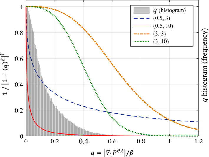
Example of a histogram of the normalized gradient information for a view angle θ in a specific direction (b = 1) overlaid with brightness gradient functions parameterized by various (δ, γ) pairs. [Color figure can be viewed at wileyonlinelibrary.com]
Finally, it was empirically determined that eight iterations gave good results for the input noise level associated with the exposure level and phantom used in this study. Therefore, in this work, the iterations were fixed at this value for all view angles.
2.A.4. Filter parameterization
As these three filters have been described in detail in the previous sections, it is clear that each filter has only a few free parameters. For the boxcar filter, the only free parameter is s and results were analyzed for s = {2, 3, 4, 5, 6, 7}. For the ATM filter, the free parameters are W 0, p l , and p h . For the data acquired in this work, after empirical optimization, W 0 = 5 showed good results and it was therefore fixed at this value. For AD, the free parameters are δ and γ (since β was calculated, and the number of iterations was fixed). The parameter spaces were sampled with 106 and 100 operating points for ATM and AD, respectively.
2.B. Physical phantom data acquisition
In this study, the chest region at the shoulder's level of an anthropomorphic pediatric phantom (ATOM 10‐year‐old phantom, Model 706, CIRS Inc., Norfolk, VA) was scanned using a benchtop CBCT imaging system (Fig. 3). This imaging system consists of a rotating anode x‐ray tube (Varian G‐1592, Salt Lake City, UT) and a flat panel energy‐integrating detector (EID) (PaxScan 4030CB, Varian, Salt Lake City, UT). This detector has an active area of 30 × 40 cm containing an array of 2,048 × 1,536 detector elements with a native pixel pitch of 194 μm which were binned under a 2 × 2 scheme during acquisition.
Figure 3.
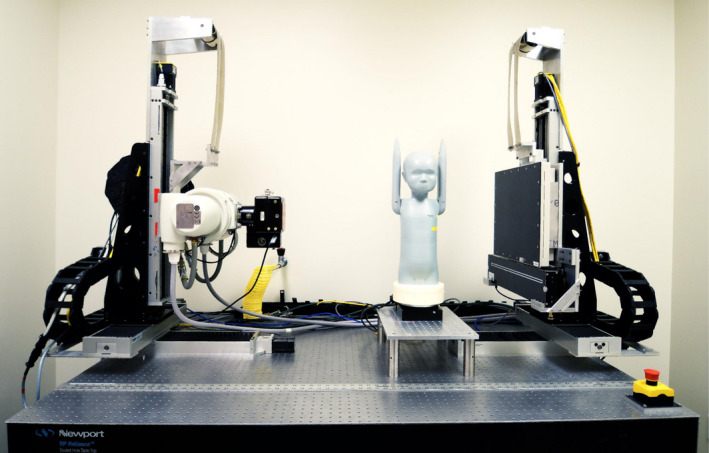
Experimental setup: benchtop CBCT imaging system and anthropomorphic phantom. [Color figure can be viewed at wileyonlinelibrary.com]
The source‐to‐isocenter distance was 766 mm, and the source‐to‐detector distance was 1,163 mm. The beam collimation at the detector plane was 130 × 111 mm in the row and column directions, respectively. The tube potential was set at 70 kVp, and no bowtie filter was used, but the beam was hardened with a 1 mm Cu filter. Two exposure levels were used, 520 and 130 mAs, corresponding to 1.9 and 0.5 mGy, respectively. These doses were determined using a conventional CTDIvol measurement with the 16 cm CTDI phantom. Fifty repeated scans were performed at each dose level in order to perform the image quality measurements described in the next section. The CBCT system was operated under the pulsed fluoro‐mode with a pulse width of 8 ms and a detector readout of 30 frames/s. The object was rotated at 10°/s and a full scan dataset of 360° was acquired for each scan. The image acquisition process was automated and synchronized to assure repeatability between scans.
Once the raw data were acquired, it underwent LSC through each of the filtering methods in this work, followed by image reconstruction. CT image reconstruction was performed using the Feldkamp–Davis–Kress (FDK) algorithm22 and a band‐limited ramp kernel without any apodization. Reconstructed CT images had a voxel size of 0.19 × 0.19 × 0.47 mm3. The small in‐plane image resolution was required for measurements of non‐aliased noise at the current detector binning level. An empirical beam hardening correction scheme23 was applied to mitigate the beam hardening artifacts. The three LSC methods were implemented in MATLAB (The MathWorks Inc., Natick, MA). Denoising the raw count volumes using the current implementations took 9 s for the boxcar, 23–26 s for ATM (parameter dependent), and 38 s for AD. However, these comparisons in efficiency are limited since further improvements are possible such as additional parallelizability and using a lower level processing language. Image reconstruction was performed in C++.
2.C. Frequency‐dependent image quality metrics
In this work, spatial resolution and noise measurements were explored across the parameter space for both LSC methods. Spatial resolution and noise were characterized locally in order to account for the potential shift‐variant behavior introduced by the given image object and LSC method. Local 2D NPS and 2D MTF measurements were performed at two characteristic spatial locations in the central slice within the phantom [Fig. 6(a)]: (a) posterior: corresponding to a highly photon‐starved region along the path of largest attenuation and (b) anterior: corresponding to a region located further from the photon‐starved measurements. Repeated scans were acquired to assess noise performance. These also facilitate the spatial resolution measurements by removing noise from the mean image without affecting the inherent blurring mechanisms.
Figure 6.
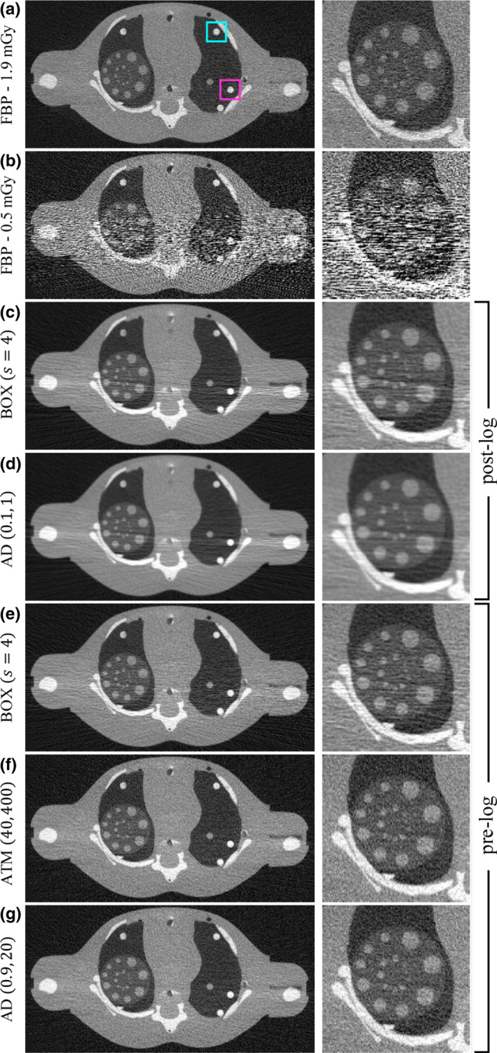
Full FOV (214 × 109 mm2) and zoomed ROI (58 × 58 mm2) images. (a) 1.9 mGy without LSC, (b) 0.5 mGy without LSC, post‐log (c, d), and pre‐log (e, f, g) corrections for low‐dose image. Parameters for each method are indicated [ATM: (p l , p h ), AD: (δ, γ)]. Images displayed with W/L = 2500/0 HU. Subfigure (a) shows posterior (magenta) and anterior (cyan) locations for image quality measurements. [Color figure can be viewed at wileyonlinelibrary.com]
2.C.1. Noise
Experimental local 2D NPS measurements can be performed by using the ensemble of reconstructed CT images from the repeated scans,24 and can be mathematically described as
| (14) |
where N x × N y is the ROI matrix size (57 × 57), ∆x = ∆y corresponds to the CT image pixel size (0.19 × 0.19 mm), DFT represents the 2D discrete Fourier transform, and is the average ROI image obtained from R = 50 repeated scans. The noise magnitude, denoted as σ, was also calculated as the square root of the area under the 2D NPS.
Figure 4 shows how noise coarseness and directionality can be measured. First, radial profiles (1D NPS) at each angle θ are extracted from the 2D NPS (a total of N θ spokes). For the coarseness analysis, the mean frequency (horizontal axis value, k) for each spoke is plotted as a function of angle in the polar plot. For the directionality assessment, the areas under the 1D NPS curves, defined as A(θ), are first normalized with respect to the maximum area, A max, and then the normalized areas are plotted as a function of angle. An additional scalar metric for NPS directionality, which is referred to as the “isotropy score” and denoted ϵ NPS, can be obtained by calculating the average radius of the directionality plot, i.e., ε NPS = 〈r〉 = 〈A(θ)/A max〉. Because , the following intuitive relationship is readily apparent:
| (15) |
Figure 4.
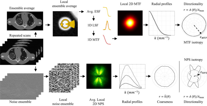
Workflow to measure local 2D NPS and 2D MTF. Coarseness and directionality of the 2D NPS and the directionality of the 2D MTF can also be extracted as 1D metrics. The 0D isotropy score, ϵ, is the average radius of the directionality of either the NPS or MTF. [Color figure can be viewed at wileyonlinelibrary.com]
Thus, isotropy is a measure of how uniformly the noise is distributed around 2π. A perfectly isotropic NPS would have a value of ϵ NPS = 1. Any measure of anisotropy in the NPS leads to a value less than 1, with a minimum occurring at 1/N θ for the most anisotropic NPS possible. Finally, contour maps of noise magnitude (standard deviation, σ) and ϵ NPS were plotted across the parameter spaces of each LSC method.
2.C.2. Spatial resolution
The spatial resolution performance of an imaging system is usually assessed by measuring the PSF or the MTF. In this work, the 2D MTF was measured as shown in the diagram from Fig. 4. Repeated scans were averaged in the image domain to obtain a “noiseless” estimate of the image object. Since photon starvation is a stochastic process, any associated noise streaks present in individual images are considerably mitigated by this approach and facilitate the measurement of spatial resolution. The rods in the posterior and anterior regions had the same high contrast (posterior = 1442 ± 43 HU, anterior = 1427 ± 46 HU). While the contrast dependence of the LSC methods was out of the scope of this work, very high contrast was used because the resolution measurement is more reliable at such low dose. Additionally, rods were suitable for these measurements because the analysis was limited to 2D. For the measurement of each of the rods in the mean image, noise reduction was performed for both the interior of the rod and the lung background, but not the edge of the rod itself.25 The interior and exterior regions were both defined 3–5 image pixels away from edge. Then, 3.5 mm long radial edge profiles were extracted around 360 degrees with an angular step size of 1 degree. Next, a low noise edge spread function (ESF) for each angle was found by radially averaging all the profiles within a span of −30 and +30 degrees. This approach is valid under the assumption that the local variability between edge profiles extracted at adjacent angles is low. Next, each average ESF was differentiated and fitted to a Gaussian function to obtain an upsampled 1D line spread function (LSF). Subsequently, the 1D Fourier transform was performed to obtain the respective 1D MTF, and the 2D MTF was formed by assembling all of the radial 1D MTFs and interpolating between them to fill in the missing data.
Additionally, for the 1D MTF along the k x and k y axes, the frequency where the MTF fell to 10% was determined. These values serve as 0D surrogates of the spatial resolution and were denoted as MTF10/x and MTF10/y. Finally, the 2D MTF underwent the same directionality analysis as the 2D NPS with the respective isotropy scores denoted as ϵ MTF (the analogous interpretation to Eq. (15) is how uniformly the area under the 2D MTF is distributed in 2π). Contour maps of MTF10/x, MTF10/y, and ϵ MTF were also plotted across the parameter spaces of each LSC method.
2.C.3. Validation
To validate the benchtop system and these measurement methodologies, noise and spatial resolution measurements were performed for a custom‐made cylindrical breast phantom (Gammex, Middletown, WI) acquired at high dose and reconstructed using FBP. Figure 5 demonstrates that the NPS and MTF are both isotropic under these conditions and serves as a benchmark for the benchtop system. When changing to the anthropomorphic pediatric phantom used in this work, several effects are understood for FBP reconstructions: (a) the NPS is very anisotropic because the phantom is highly heterogeneous, but (b) the noise coarseness is still constant in every direction, and (c) the MTF is still isotropic. Given this benchmarking of the CT system, the full impact of LSC applied to the raw counts domain will have been isolated.
Figure 5.
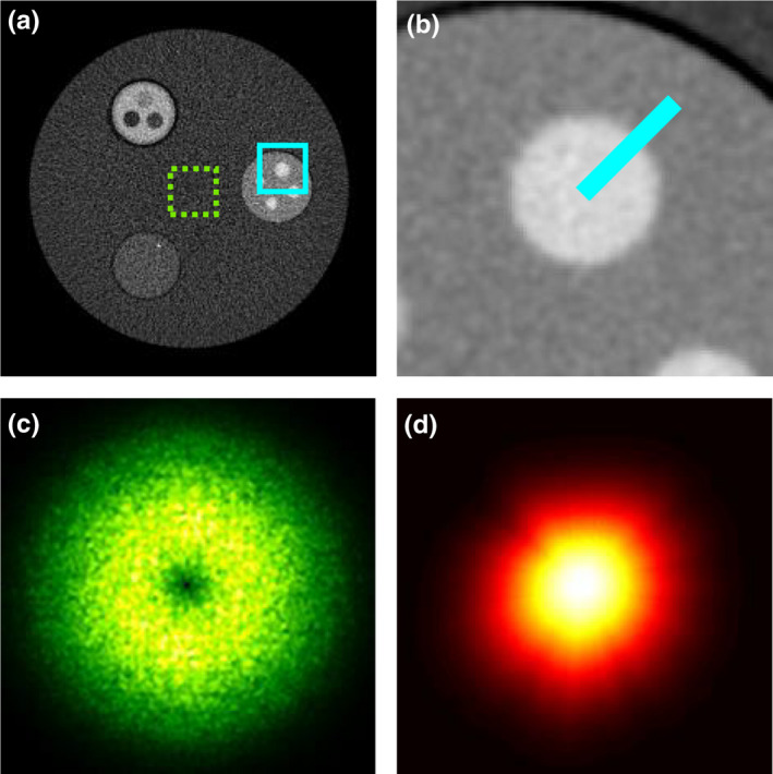
(a) Gammex breast phantom with ROIs where noise (dashed) and resolution (solid) were measured, (b) ROI in the mean image, (c) 2D NPS, (d) 2D MTF. [Color figure can be viewed at wileyonlinelibrary.com]
3. Results
3.A. Qualitative assessment
Figure 6 shows reconstructed images. Full FOV images are shown in the left column, and zoomed‐in images of a region‐of‐interest (ROI) in the right lung are shown in the right column. Object features are clearly visible in the 1.9 mGy image without LSC [Fig. 6(a)]. However, noise streaks across the L/R axis of the phantom (≈20 cm) in the 0.5 mGy image without LSC [Fig. 6(b)] obstruct most of the smaller rods in the lungs and make it difficult to resolve bone edges in the scapula, spine, and humerus. Figures 6(c)–6(g) are each corrections for the low‐dose image. To validate selection of the pre‐log domain over the post‐log domain for correction, images were first generated using correction in the post‐log domain with many different parameterizations of the BOX and AD filters (ATM was not included since it is not directly applicable to the post‐log domain). Figures 6(c), 6(d) correspond to the parameterizations in the post‐log domain that yielded the best subjective image quality and therefore demonstrate why performing correction in this domain is insufficient to remove noise streaks. For correction in the raw counts domain, the BOX image [Fig. 6(e)] also still has residual streaks. However, both the nonlinear methods — ATM and AD [Figs. 6(f), 6(g)] — are successful in removing noise streaks while preserving to some extent spatial resolution.
3.B. Noise performance
Figures 7(a), 7(c) show how noise magnitude, σ, and noise isotropy scores, ϵ NPS, vary as a function of s for BOX images for both the anterior and posterior spatial locations. Values at s = 1 correspond to the image without correction [Fig. 6(b)]. The s = 4 image is analyzed in more detail in the first row of Fig. 12 which contains: a noise only image (subfigures a, d); 2D NPS (subfigures b, e); and coarseness plots (subfigures c, f). Additionally, the coarseness curve for a given spatial location from the 1.9 mGy image without LSC is also overlaid in Figs. 12(c) and 12(f) for comparison. For the images without LSC, coarseness plots have a constant mean frequency (≈1 mm−1) in every direction despite topological variation observed in the 2D NPS (shown in Fig. 4).
Figure 7.
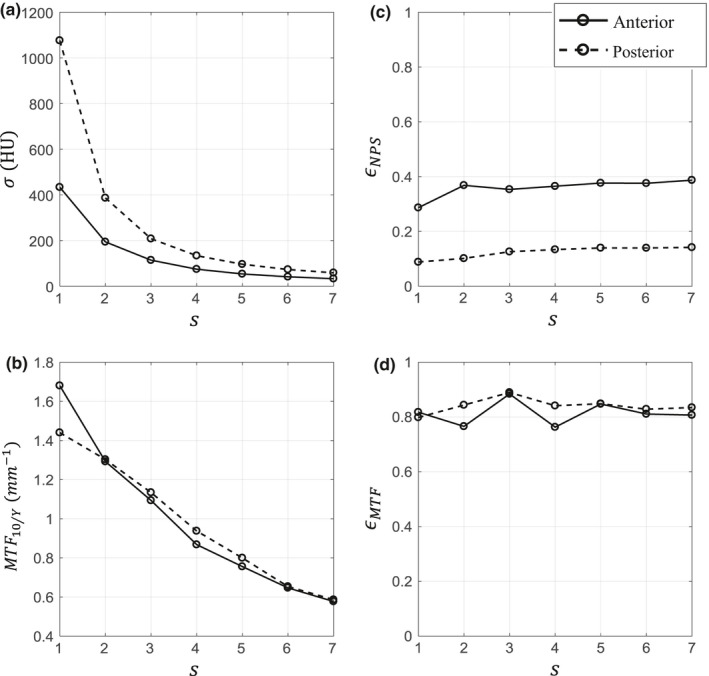
Zero‐dimensional image quality metrics across the parameter space for BOX images at 0.5 mGy. s = 1 corresponds to the FBP image without LSC [Fig. 6(b)].
Figure 12.
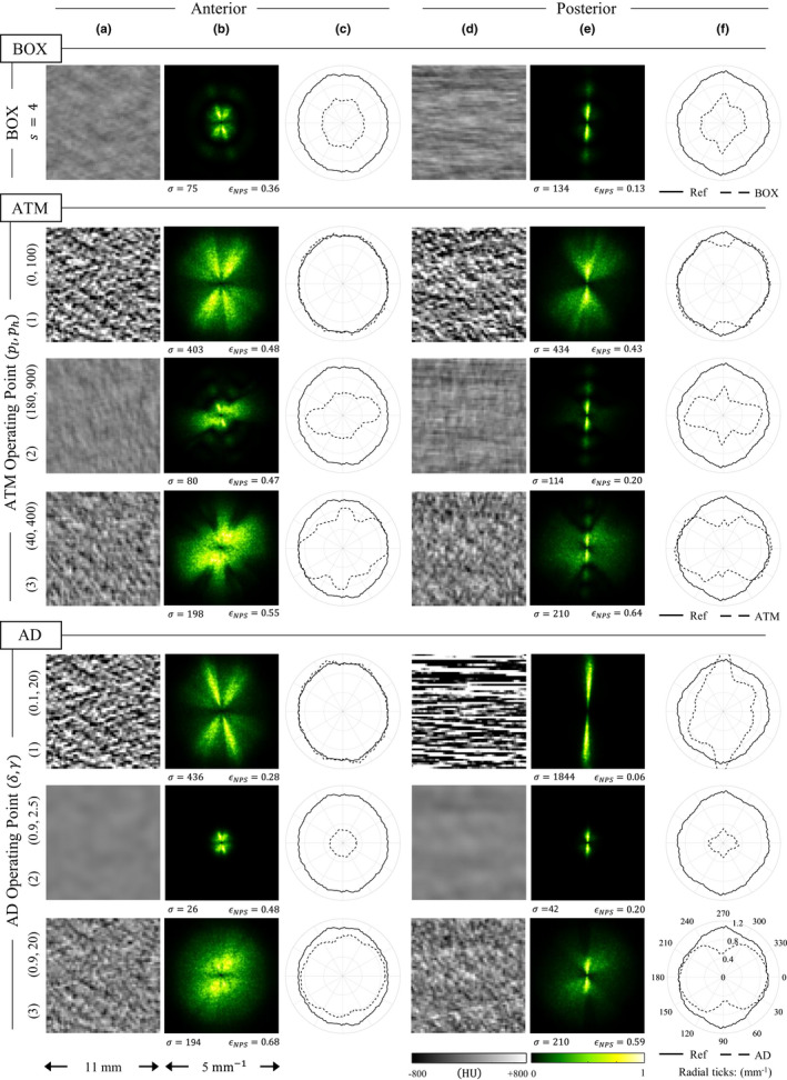
Noise measurements for BOX, ATM, and AD images. One example of the boxcar filter is provided, while three operating points for each nonlinear filter are also shown as examples, corresponding to those indicated by the markers in Figs. 8 and 9. For both anterior and posterior ROIs, three figures are shown: (a, d) the local noise only image, (b, e) normalized 2D NPS, and (c, f) coarseness plots. The coarseness curve for the given ROI obtained at 1.9 mGy without LSC is also shown for reference. Values of noise magnitude, σ (HU), and NPS isotropy, ϵ NPS , for each case are also provided. [Color figure can be viewed at wileyonlinelibrary.com]
Figure 8 shows how the noise performance varies across the 2D parameter space of ATM for both spatial locations. Figures 8(a) and 8(b) display the noise magnitude, and Figs. 8(c) and 8(d) show the isotropy scores. The three operating points that are indexed and overlaid in Fig. 8(b) are analyzed in more detail in Fig. 12.
Figure 8.
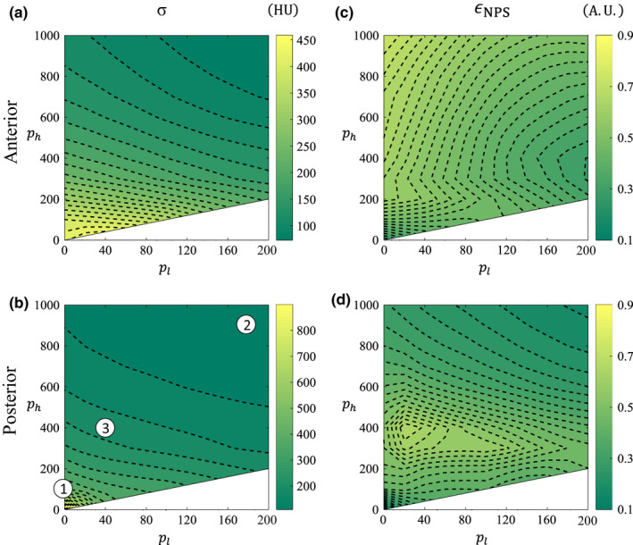
Noise contour maps in ATM‐space for the anterior and posterior spatial locations. (a, b) Noise standard deviation, σ, in HU. (c, d) NPS isotropy, ϵ NPS . Indexed parameters in (b) correspond to rows in Fig. 12. Note that ATM is not defined in the white space where p h < p l . [Color figure can be viewed at wileyonlinelibrary.com]
Results for the noise performance of the AD filter follow an analogous presentation as the ATM filter. Figure 9 shows how the noise performance varies across the 2D parameter space of AD, and the three operating points that are indexed and overlaid in Fig. 9(b) are analyzed in more detail in Fig. 12.
Figure 9.
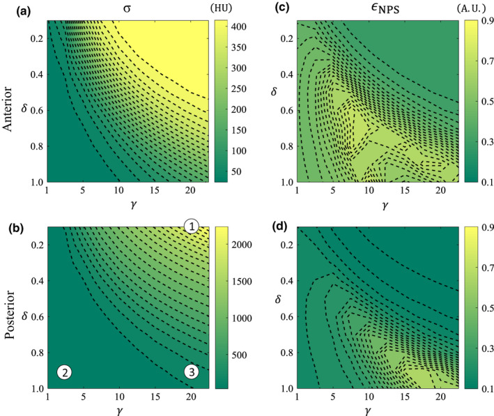
Noise contour maps in AD‐space for the anterior and posterior spatial locations. (a, b) Noise standard deviation, σ, in HU. (c, d) NPS isotropy, ϵ NPS . Indexed parameters in (b) correspond to rows in Fig. 12. [Color figure can be viewed at wileyonlinelibrary.com]
3.B.1. Noise magnitude
The noise magnitude, σ, for BOX images decreases as s increases [Fig. 7(a)]. This is a natural result. For the ATM method [Figs. 8(a), 8(b)], noise magnitude decreases rapidly when moving from low to high p l and p h values. This is expected, since whenever p l or p h is increased, there is more smoothing in the raw domain and thus lower noise in the reconstructed image. This trend can best be explained using Fig. 1 and Eq. (6). Increasing either p l or p h means that for a given signal level, both a larger spatial window and less data trimming will be applied. Since the contours are approximately linear with a slope of −1, this means that the noise reduction is approximately equal per unit of p l or p h increase. This slope is slightly larger than −1 due to the fact that increasing p h has the added effect that more of the higher signal levels are also being filtered. These trends are true for both spatial locations.
A similar observation can be described for the AD method [Figs. 9(a), 9(b)]. There is a decrease in noise magnitude when moving from low δ and high γ to high δ and low γ. This trend can best be explained using Fig. 2. Brightness gradient functions with small δ and large γ have a short plateau and rapid fall, and will therefore provide hardly any filtration of the raw data. On the other hand, functions with large δ and small γ have a long plateau and a more gradual fall and will therefore filter more of the data in the raw domain leading to lower noise images.
3.B.2. Noise directionality and coarseness
Despite decreasing noise magnitude with increasing s, the noise isotropy, ϵ NPS, for BOX images remains relatively flat, only increasing from 0.09 to 0.14 in the posterior or from 0.29 to 0.39 in the anterior regions [Fig. 7(c)]. This indicates streaks are still present and this is validated in the reconstructed image [Fig. 6(e)] and by the 2D NPS [Figs. 12(b), 12(e)].
For both nonlinear LSC methods, the NPS isotropy contour maps (Figs. 8 and 9) demonstrate a more complex dependence across parameter space. The NPS of the CT image without LSC (not shown) is highly anisotropic in the posterior ROI because of noise streaks. The analogous operating point for an uncorrected CT image in the ATM‐space is at the bottom left corner (p l , p h ) = (0, 0), where ϵ NPS = 0.11 for the posterior ROI. The ATM filter is able to increase the NPS isotropy to as high as 0.67 in the island near (p l , p h ) = (20, 400). For the anterior ROI, the isotropy is higher overall compared to the posterior ROI since the value at (p l , p h ) = (0, 0) was already 0.29. The highest isotropy value for this ROI is 0.73 occurring near (p l , p h ) = (0, 1000). For both spatial locations therefore, a high isotropy was observed at small p l ‐values, but there is a spatial location dependence for p h .
In the case of the AD method, the NPS isotropy trends do not change as a function of spatial location, but the magnitude of the metric is higher for the anterior region than the posterior one. The analogous operating point for an uncorrected CT image in the AD‐space is at the top right corner. Operating points with high NPS isotropy occur at high values of δ and high values of γ.
NPS isotropy is related to the noise magnitude by Eq. (15). However, because A max may differ for LSC images with the same noise magnitude (i.e., the noise is distributed differently), the ϵ NPS contours are not the same shape as the σ contours.
The noise coarseness for BOX images is reduced isotropically [Fig. 12(c), 12(f)]. However, noise coarseness for the ATM and AD filters is reduced anisotropically. While the mean noise frequencies can sometimes be preserved in directions parallel to the streaks, they are lower in directions perpendicular to the streaks.
3.C. Spatial resolution performance
Figures 7(b), 7(d) shows how the spatial resolution metrics — the MTF10/y value extracted along the k y axis and the resolution isotropy, ϵ MTF — vary as a function of s for BOX images for both the anterior and posterior spatial locations. The image for s = 4 is analyzed further in Fig. 13 which contains: ROIs of the high‐contrast rod used for measurement (subfigures a, d); the 2D MTF (subfigures b, e); and 1D MTF curves in the positive k x and positive k y directions (subfigures c, f). The radial averaged 1D MTF from the 1.9 mGy uncorrected CT image for a given spatial location is also overlaid in Figs. 13(c) and 13(f) for comparison.
Figure 13.
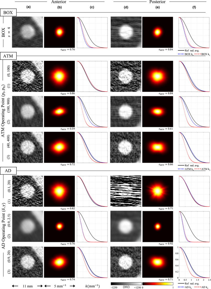
Spatial resolution measurements for BOX, ATM, and AD images. One example of the boxcar filter is provided, while three operating points for each nonlinear filter are also shown as examples, corresponding to those indicated by the markers in Figs. 10 and 11. For both anterior and posterior ROIs, three figures are shown: (a, d) ROI with high contrast rod, (b, e) 2D MTF, and (c, f) 1D MTFs in the positive k x and positive k y directions. The radial averaged 1D MTF from the 1.9 mGy image without LSC is shown for reference. Values of MTF isotropy, ϵ MTF , for each case are also provided. [Color figure can be viewed at wileyonlinelibrary.com]
Figure 10 shows the variation of these metrics across the 2D parameter space of ATM. Figures 10(a) and 10(b) show MTF10/y and Figs. 10(c) and 10(d) show ϵ MTF. The same three ATM operating points from before [indicated again in Fig. 10(b)] are shown in greater detail in Fig. 13.
Figure 10.
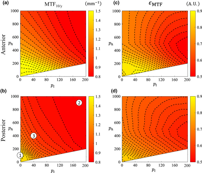
Spatial resolution contour maps in ATM‐space for the anterior and posterior spatial locations. (a, b) Spatial resolution surrogate in the y‐direction, MTF 10/y, in mm −1. (c, d) MTF isotropy, ϵ MTF . Indexed parameters in (b) correspond to rows in Fig. 13. [Color figure can be viewed at wileyonlinelibrary.com]
Figure 11 shows the spatial resolution performance across the parameter space of AD. Figures 11(a) and 11(b) show MTF10/y and Figs. 11(c) and 11(d) show ϵ MTF. The same three AD operating points from before [indicated again in Fig. 11(b)] are shown in greater detail in Fig. 13.
Figure 11.
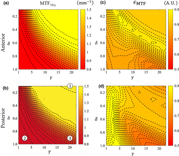
Spatial resolution contour maps in AD‐space for the anterior and posterior spatial locations. (a, b) Spatial resolution surrogate in the y‐direction, MTF 10/y, in mm−1. (c, d) MTF isotropy, ϵ MTF . Indexed parameters in (b) correspond to rows in Fig. 13. [Color figure can be viewed at wileyonlinelibrary.com]
3.C.1. Spatial resolution MTF10/y
The limiting resolution surrogate, MTF10/y, for BOX images decreases as s increases for both posterior and anterior locations [Fig. 7(b)]. This is expected since there is an accompanying noise reduction. However, the reduction is the same for both spatial locations because the boxcar filter is shift‐invariant. Figures 10 and 11 show that for both the ATM and AD filters, there is also a dependence of spatial resolution on the filter parameters, and also a more complex dependence on the spatial location in the image. As noted previously, there is more noise reduction in ATM when either p l or p h is increased. As a result, there is a corresponding loss in spatial resolution along these axes and this is true for both spatial locations [Figs. 10(a) and 10(b)]. However, the spatial resolution loss is not equal in the two spatial locations — the directions of the spatial resolution contours for both ROIs are oblique to each other. This is because the ATM filter depends on the magnitude of the raw signal itself. Therefore, if there is a small change in the filter parameters, the resulting changes in image spatial resolution will be different in photon‐starved regions than the spatial resolution changes for less attenuating regions.
For AD, there is more denoising if δ increases and γ decreases. Figures 11(a) and 11(b) confirm the associated spatial resolution loss when these parameters are changed this way. In fact, the spatial resolution contours are inversely related to the noise contours observed in Figs. 9(a) and 9(b). Additionally, the contours for the anterior and posterior directions are in the same direction. This is a convenient feature of AD, since it means that the trade‐off between noise and spatial resolution is smooth and the magnitude of the degradations is approximately the same for different spatial locations. In contrast to ATM, AD has this property because the filter in AD depends on the magnitude of the gradient of the raw signal instead of the signal itself.
3.C.2. Spatial resolution directionality
The MTF isotropy score for the CT image without LSC was ϵ MTF = 0.80 (posterior) and ϵ MTF = 0.82 (anterior). BOX images maintain this constant ϵ MTF value as s is increased [Fig. 7(d)], despite a decrease in the spatial resolution magnitude [Fig. 7(b)]. This is because the boxcar filter reduces spatial resolution equally in all directions. The first row of Fig. 13 clearly demonstrates this isotropic nature for s = 4.
For both the ATM and AD methods, the MTF isotropy contour maps (Figs. 10 and 11) have contours that behave differently than the MTF10/y contour maps. This is because the isotropy contours absorb the behavior of all the directions, and the contours of MTF10/θ in any given direction θ would have either different magnitudes, different shapes, or both. Interestingly, the MTF isotropy for ATM now has similarly shaped contours for the anterior and posterior directions [Figs. 10(c), 10(d)], despite having MTF10/y contours that differed in both magnitude and shape. The MTF isotropy for AD also has similarly shaped contours for the anterior and posterior directions [Figs. 11(c), 11(d)]; MTF10/y contour maps for AD had contours that differed in magnitude but not shape.
Resolution isotropy scores were generally smaller than the uncorrected image across the ATM parameter space because this filter always reduces spatial resolution unequally in different directions (e.g., contours of MTF10/y have different shape than MTF10/x) . AD isotropy was less than, equal to, or greater than the isotropy obtained for the uncorrected CT images; however, the shape of these contours was generally the same for different directions.
3.D. Spatial resolution and noise interplay
The trade‐off between noise and spatial resolution for BOX images has been discussed and remains relatively clear. Figure 7 and the first row of Figs. 12 and 13 show that noise and resolution are reduced isotropically for a linear filter and as such it is insufficient to remove noise streaks.
The three operating points of ATM or AD in Figs. 12 and 13 were selected to be representative of the potential within each of the parameter spaces to provide different levels of denoising. For each filter, the first row corresponds to cases where there was minimal filtration. The second row corresponds to a large amount of filtration and hence excessive blurring. Finally, the third row was selected to balance the trade‐off between noise and spatial resolution.
For the images where filtration was minimal, the spatial resolution does not change significantly from the low‐dose image without LSC. For both ATM and AD in the anterior position, the k x and k y 1D MTFs are the same as the radial average 1D MTF from the reference image [Fig. 13(c)]. Subsequently, the noise coarseness is preserved here [Fig. 12(c)]. In the posterior position, there is a slight drop in k y resolution for ATM [Fig. 13(f)] accompanied by a small decrease in noise coarseness along this same direction [Fig. 12(f)]. For AD, resolution is actually enhanced, but the streaks are nevertheless unacceptable here [Figs. 12(d)–12(f)].
The reduction in spatial resolution accompanied by a decrease in noise coarseness along the same direction can be observed for the other two operating points as well (second and third row of each filter in Figs. 12 and 13). For these cases, the larger the reduction in resolution, the larger the drop in noise coarseness. These reductions are also highly anisotropic. Because the filters reduce noise frequencies along the k y axis more than the k x axis, spatial resolution is also reduced more along the k y axis than it is along the k x axis. This can be seen in the LSC images by the separation of the 1D MTFs [Figs. 13(c), 13(f)].
Interestingly, for the operating points in the third row for ATM or AD with good noise‐resolution trade‐off, the coarseness and resolution along the k y direction are reduced, but for the most part these noise frequencies and MTF are both preserved along the k x direction. Because of this anisotropic behavior, the NPS isotropy scores are higher and the MTF isotropy scores are lower than the uncorrected image. The impact of the noise‐resolution trade‐off for these operating points is best observed in the noise only images [Figs. 12(a), 12(d)], where the noise appears less directional in the third row than in the first row, and in the ROI images for these operating points [Figs. 13(a), 13(d)], where signal along the vertical direction is observed to be leaking out while the horizontal direction has a well‐defined edge.
4. Discussion
In this work, the noise and spatial resolution characteristics of low‐dose CBCT via LSC in the raw counts domain with the AD and ATM filters were systematically investigated. It was found that these LSC methods were able to reduce noise streaks in the reconstructed CT image effectively when compared to linear filters and/or denoising in the post‐log domain. It was also found that their success depended strongly on the filter parameters used. Additionally, the images reconstructed from raw data corrected using ATM or AD presented highly anisotropic and shift‐variant noise and spatial resolution properties. Specifically, three major aspects about the imaging performance of the investigated LSC methods in terms of noise and spatial resolution can be highlighted: (a) noise magnitude and spatial resolution along the direction perpendicular to the noise streaks are inversely related, (b) noise directionality is independent of noise magnitude, and (c) noise coarseness and spatial resolution directionality have an intrinsic direct relationship.
The behavior highlighted in (a) agrees with qualitative observations from previous work with ATM and other noise streaks reduction methods.2, 8 Even though noise magnitude could be reduced considerably and the spatial resolution along the direction parallel to the noise streaks was preserved to some extent, there was still some degradation of spatial resolution along the perpendicular direction. The point in (b) highlights the importance of taking into account noise directionality; it was observed that a NPS with the same magnitude could have different degrees of isotropy. This is important since image feature conspicuity can be influenced by the directionality of the noise texture.24 Finally, the point in (c) highlights the relationship between noise coarseness and MTF isotropy. It was observed that for a given spatial location in the FOV, the preferential denoising along photon‐starved view angles resulted in a lower mean noise frequency along these same directions, which directly correlated with degradation of the spatial resolution along these directions. In other words, the coarseness plots mimic the topography of the 2D MTF, and any anisotropic reduction of noise coarseness would be reflected by a decrease in the MTF isotropy as well. These findings agree with previous work done with penalized likelihood reconstruction26 where a similar complementary behavior between the MTF and the NPS was also observed.
This work has some limitations. The imaging performance assessment was limited to 2D. Analyzing the imaging performance across slices would be relevant since the LSC methods implemented in this work process the raw data two‐dimensionally at the detector plane, not just along the row direction. However, this would only impact the noise properties, not the spatial resolution since the phantom used in this study is uniform along the slice direction. Additionally, even though the ensemble averaging approach enables the measurement of noise and spatial resolution in highly nonlinear CT systems, its accuracy for severely photon‐starved scenarios may depend strongly on the amount of repeated scans, particularly for uncorrected raw data with streaky CT images. This large amount of repeated scans may not be practical, particularly if multiple imaging scenarios are considered for imaging performance assessment. However, these kinds of rigorous studies with repeated physical data for a given phantom may serve as a basis to validate future numerical simulation studies or theoretical models that can facilitate the prediction of the behavior of noise and spatial resolution at different operating points within the filter parameter space and spatial locations.
The extent of the imaging performance assessment in Part I of this work was limited to noise and spatial resolution. Figures 7, 8, 9, 10, 11, 12, 13 provide an overall understanding of the noise and spatial resolution performance for each filter, but what conclusions can be drawn so that optimal filter parameters can be chosen? Is it best to have an isotropic NPS at the expense of a highly anisotropic MTF? Or should spatial resolution remain isotropic without any regard to the texture of the NPS? Should certain spatial locations within the image have more favorable properties than others? Is one filter better than the other? Final consideration of the noise and spatial resolution metrics in Part I suggests that it is challenging to choose optimal parameters that capture all of the favorable properties of any single metric when considered on its own. In other words, no clear optimal point stands out. Optimizing parameter selection based on noise standard deviation σ or limiting spatial resolution MTF10 would lead to one operating on the boundaries of the parameter space. Alternatively, optimizing based on the isotropy of the NPS or MTF might favor one spatial location in the image FOV over another.
Therefore, while a detailed quantitative assessment of noise and spatial resolution provides a foundation to understand the imaging performance of a given LSC method, in order to properly select optimal parameters, this process needs to be targeted to a given imaging task. This approach is taken in Part II15 of this work where a task‐based detectability framework incorporates the noise and spatial resolution properties simultaneously for an imaging task of interest.
5. Conclusion
Performance of LSC schemes in low‐dose CBCT was investigated using the AD and ATM filters in the raw counts domain. For each filter, the parameter space was extensively sampled and assessed using frequency‐dependent image quality metrics of noise and spatial resolution. The noise and spatial resolution characteristics of the LSC schemes are highly anisotropic and shift‐variant. A simple parameter optimization based solely upon the noise and spatial resolution characteristics may be difficult. Instead, a task‐based detectability framework is required to fully capture the imaging performance of either LSC method and to optimize the parameter selection for the filters, and this will be discussed in Part II of this work.15
Conflict of Interest
The authors have no conflicts to disclose.
Acknowledgments
This work is partially supported by an NIH grant R01CA169331 and by a research contract with GE Healthcare. The authors thank Dr. Michael Speidel for providing the pediatric phantom used for the experimental studies.
References
- 1. Lin EC. Radiation risk from medical imaging. Mayo Clin Proc. 2010;85:1142–1146. [DOI] [PMC free article] [PubMed] [Google Scholar]
- 2. Hsieh J. Adaptive streak artifact reduction in computed tomography resulting from excessive x‐ray photon noise. Med Phys. 1998;25:2139–2147. [DOI] [PubMed] [Google Scholar]
- 3. Kelm ZS, Blezek D, Bartholmai B, Erickson BJ. Optimizing non‐local means for denoising low dose CT. in Proc. IEEE Int. Symp. Biomed. Imaging; 2009, pp. 662–665.
- 4. Chen Y, Chen W, Yin X, et al. Improving low‐dose abdominal CT images by weighted intensity averaging over large‐scale neighborhoods. Eur J Radiol. 2011;80:e42–e49. [DOI] [PubMed] [Google Scholar]
- 5. Li Z, Yu L, Trzasko JD, et al. Adaptive nonlocal means filtering based on local noise level for CT denoising. Med Phys. 2014;41:011908. [DOI] [PubMed] [Google Scholar]
- 6. Kachelrieß M, Watzke O, Kalender WA. Generalized multi‐dimensional adaptive filtering for conventional and spiral single‐slice, multi‐slice, and cone‐beam CT. Med Phys. 2001;28:475–490. [DOI] [PubMed] [Google Scholar]
- 7. Li T, Li X, Wang J, et al. Nonlinear sinogram smoothing for low‐dose x‐ray CT. IEEE Trans Nucl Sci. 2004;51:2505–2513. [Google Scholar]
- 8. Rivi`ere PJL, Billmire DM. Reduction of noise‐induced streak artifacts in X‐ray computed tomography through spline‐based penalized‐likelihood sinogram smoothing. IEEE Trans Med Imag. 2005;24:105–111. [DOI] [PubMed] [Google Scholar]
- 9. Wang J, Li T, Lu H, Liang Z. Penalized weighted least‐squares approach to sinogram noise reduction and image reconstruction for low‐dose x‐ray computed tomography. IEEE Trans Med Imag. 2006;25:1272–1283. [DOI] [PMC free article] [PubMed] [Google Scholar]
- 10. Manduca A, Yu L, Trzasko JD, et al. Projection space denoising with bilateral filtering and CT noise modeling for dose reduction in CT. Med Phys. 2009;36:4911–4919. [DOI] [PMC free article] [PubMed] [Google Scholar]
- 11. Perona P, Malik J. Scale‐space and edge detection using anisotropic diffusion. IEEE Trans Patt Anal Mach Intell. 1990;12:629–639. [Google Scholar]
- 12. Demirkaya O. Reduction of noise and image artifacts in computed tomography by non‐ linear filtration of the projection images. Proc SPIE. 2001;4322:917–923. [Google Scholar]
- 13. Yu L, Vrieze TJ, Leng S, Fletcher JG, McCollough CH. Technical note: measuring contrast‐ and noise‐dependent spatial resolution of an iterative reconstruction method in CT using ensemble averaging. Med Phys. 2015;42:2261–2267. [DOI] [PMC free article] [PubMed] [Google Scholar]
- 14. Li K, Gomez‐Cardona D, Hsieh J, Lubner MG, Pickhardt PJ, Chen G‐H. Statistical model based iterative reconstruction in clinical CT systems. Part III. Task‐ based kV/mAs optimization for radiation dose reduction. Med Phys. 2015;42:5209–5221. [DOI] [PMC free article] [PubMed] [Google Scholar]
- 15. Gomez‐Cardona D, Hayes JW, Zhang R, Li K, Cruz‐Bastida JP, Chen GH. Low‐dose cone‐beam CT via raw counts domain low‐signal correction schemes: Performance assessment and task‐based parameter optimization (Part II: Task‐based parameter optimization). Med Phys. 2018;45:1957–1969. [DOI] [PMC free article] [PubMed] [Google Scholar]
- 16. Restrepo A, Bovik AC. Adaptive trimmed mean filters for image restoration. IEEE Trans Audio Speech Lang Process. 1988;36:1326–1337. [Google Scholar]
- 17. Catt′e F, Lions P‐L, Morel J‐M, Coll T. Image selective smoothing and edge detection by nonlinear diffusion. SIAM J Num Anal. 1992;29:182–193. [Google Scholar]
- 18. Whitaker R, Pizer S. A multi‐scale approach to nonuniform diffusion. Comput Vis Image Und. 1993;57:99–110. [Google Scholar]
- 19. Weickert J, Romeny BMTH, Viergever MA. Efficient and reliable schemes for nonlinear diffusion filtering. IEEE Trans Image Process. 1998;7:398–410. [DOI] [PubMed] [Google Scholar]
- 20. Weickert J. Anisotropic Diffusion in Image Processing. Stuttgart: Teubner; 1998. [Google Scholar]
- 21. Gomez‐Cardona D, Hayes J, Zhang R, Li K, Cruz‐Bastida JP, Chen G‐H. Low signal correction scheme for low dose CBCT: the good, the bad, and the ugly. Proc SPIE. 2017;10132:101320Z–101320Z‐7. [Google Scholar]
- 22. Feldkamp LA, Davis LC, Kress JW. Practical cone‐beam algorithm. J Opt Soc Am A. 1984;1:612–619. [Google Scholar]
- 23. Kyriakou Y, Meyer E, Prell D, Kachelrieß M. Empirical beam hardening correction (EBHC) for CT. Med Phys. 2010;37:5179–5187. [DOI] [PubMed] [Google Scholar]
- 24. Gomez‐Cardona D, Li K, Lubner MG, Pickhardt PJ, Chen G‐H. Noise performance studies of model‐based iterative reconstruction (MBIR) as a function of kV, mA and exposure level: impact on radiation dose reduction and image quality. Proc SPIE. 2015;9412:941238. [Google Scholar]
- 25. Hsieh J. Computed Tomography: Principles, Design, Artifacts, and Recent Advances. Bellingham: SPIE; 2003. [Google Scholar]
- 26. Gang GJ, Stayman JW, Zbijewski W, Siewerdsen JH. Task‐based detectability in CT image reconstruction by filtered backprojection and penalized likelihood estimation. Med Phys. 2014;41:081902. [DOI] [PMC free article] [PubMed] [Google Scholar]


