Abstract
Recent advances in deep learning (DL) have provided promising solutions to medical image segmentation. Among existing segmentation approaches, the U-Net-based methods have been used widely. However, very few U-Net-based studies have been conducted on automatic segmentation of the human brain claustrum (CL). The CL segmentation is challenging due to its thin, sheet-like structure, heterogeneity of its image modalities and formats, imperfect labels, and data imbalance. We propose an automatic optimized U-Net-based 3D segmentation model, called AM-UNet, designed as an end-to-end process of the pre and post-process techniques and a U-Net model for CL segmentation. It is a lightweight and scalable solution which has achieved the state-of-the-art accuracy for automatic CL segmentation on 3D magnetic resonance images (MRI). On the T1/T2 combined MRI CL dataset, AM-UNet has obtained excellent results, including Dice, Intersection over Union (IoU), and Intraclass Correlation Coefficient (ICC) scores of 82%, 70%, and 90%, respectively. We have conducted the comparative evaluation of AM-UNet with other pre-existing models for segmentation on the MRI CL dataset. As a result, medical experts confirmed the superiority of the proposed AM-UNet model for automatic CL segmentation. The source code and model of the AM-UNet project is publicly available on GitHub: https://github.com/AhmedAlbishri/AM-UNET.
Introduction
There has been considerable attention to medical imaging technologies and applications due to their substantial benefits for medical diagnosis and treatment. In particular, there have been advances in automated medical imaging segmentation. On the other hand, the demand and interest for new medical imaging applications have grown substantially. The advancements in deep learning, especially with image segmentation technologies, have been applied to medical imaging and automated segmentation [31] for a broad range of studies, from cancer detection [13] to brain tumor segmentation [23] and treatment and prevention of brain aging-related conditions, Alzheimer’s disease (AD) [51].
The image segmentation and detection studies using Convolutional Neural Networks (CNN) [31] have shown its performance comparable to that of visual detection or segmentation performed by human operators. Segmentation tasks play a vital role in delineating different anatomical structures, and other regions [7]. However, there are still challenges in applying deep learning technologies to neuroimaging segmentation in practice. Specifically, segmentation becomes a challenging task due to the following reasons [18]:
Variations in the size and structure of the objects.
Images with different modalities, in different formats, and of different sizes due to the usage of different scanning systems.
Insufficient manually labeled data for training.
High class-imbalance in most training and evaluation datasets.
Lack of high quality of data manually annotated by domain experts.
Complicated and time-consuming task of manual segmentation.
Vulnerability to human errors during experts’ annotation.
These challenges could be amplified on more complex data, e.g., computed tomography (CT) images or magnetic resonance images (MRI), which have been used to diagnose disease for the best treatment decision [53]. In particular, an increasing number of neuroimaging studies have focused on identifying an intricate pattern or a small region in the human brain for predictive medicine. Medical imaging technologies need to handle multiple images or slices representing anatomical volumes in a specific data format acquired from imaging scanners [18]. The automated segmentation can be conducted with specific human organs (e.g., liver, brain, lung) or their boundary annotations of labeled datasets [31]. However, automated segmentation technologies are mainly developed for large cortical and subcortical areas (e.g., FreeSurfer [20]). The conventional segmentation methods have limited capacity to obtain high accuracy in segmenting small regions of medical brain images, especially those of the deep brain [49]. Therefore, it is imperative to develop more advanced automated segmentation methods that can be applied to small regions or complex and diverse data formats to facilitate various medical applications for medical research and clinical practice.
Automatic segmentation studies on small and complex brain regions have not been widely attempted. The present study focused on the claustrum (CL), an excellent example of an important and challenging target of the CNN approach. CL is a mysterious thin deep brain grey matter structure located at the center of each hemisphere. It is known as the brain’s most highly connected hub [45]. CL has reciprocal connectivity with almost all cortical and subcortical brain areas, and massive input from all significant neuromodulator circuits [44]. Based on the anatomy and animal neurophysiological findings, CL has been hypothesized as a brain network hub node for multisensory integration [35], conscious percepts [12], and bottom-up and top-down attention [22]. Studies have reported CL volume reduction in post-mortem brains in people with autism spectrum disorders [14, 48] and schizophrenia [8] and CL abnormalities in patients with neurological disorders [36, 43]. Figure 1 shows the MRI of the human brain with CL highlighted in orange.
Fig. 1.
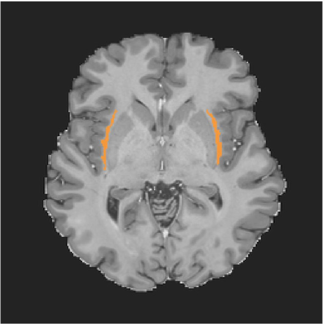
The human claustrum (orange) delineated in a T1-weighted MRI
Despite accumulating evidence of CL abnormalities in people with neuropsychiatric disorders [36, 43], few neuroimaging studies have been conducted to investigate the functions of human CL. It is primarily due to (1) the methodological limitations of conventional neuroimaging techniques to isolate the thin structure of CL (i.e., the limited spatial resolutions of MRI and other neuroimaging techniques) and (2) lack of essential neuroimaging tools (e.g., no CL label in most widely used neuroimaging brain atlases, no reliable method to delineate CL). In addition, the region of interest (ROI) approach to CL requires manual segmentation of CL using structural MR images. An earlier study developed a manual tracing protocol for volumetric analysis of the human CL [14]. However, the protocol did not provide details of CL’s unique anatomy and no clear boundary to delineate the sub-regions. Also, manual segmentation of CL on MRI’s is a time-consuming and challenging procedure that requires domain expertise.
In this paper, we propose an end-to-end mini U-Net-based network, AM-UNet, to achieve automatic 3D CL segmentation. For the training and validation of our AM-UNet network, we used the CL label maps that domain experts manually segmented. Furthermore, to improve the model accuracy while mainly reducing the training dataset, we have optimized the end-to-end workflow consisting of preprocessing, augmentation, and postprocessing. We have explored the proposed approach by experimenting with various deep learning architectures (U-Net variants) for automatic segmentation of the CL from T1, T2, and T1T2 weighted MRI datasets. Using multiple performance metrics, we extensively evaluated the model performance by comparing AM-UNet with two other state-of-the-art segmentation models. Our main contributions to this research are as follows:
Design of an optimal U-Net architecture for smaller, simpler, and efficient CL segmentation.
Development of an automated end-to-end 3D segmentation network for CL segmentation.
Robust segmentation model for multi sequences (T1, T2, and T1T2) and multi-view (Axial, Coronal, or Sagittal) MRIs from the Human Connectome Project (HCP) [46].
State-of-the-art results of automatic CL segmentation based on extensive evaluations, including those of a domain expert.
Related work
We have conducted extensive literature reviews on automated medical image segmentation. This section will first focus on medical imaging and then will discuss related work on deep learning methods for medical image segmentation.
Medical imaging
Advanced techniques for medical image formats, including Nifti, Minc, and Dicom [30], have shown excellent performance on detection of anatomies in medical search [31]. Furthermore, medical image segmentation for partitioning the areas of interest and their boundaries has shown promising results [31]. The machine learning techniques enhance the model performance, optimize the model weights while training, and remove the irrelevant aspect of the data [39]. In deep learning algorithms, the more data the algorithm trains on, the better the results it can produce [40]. The data augmentation technique is used to create more training data from the available dataset. The data augmentation is a general solution to reduce over-fitting on image data [4]. Also, obtaining a large amount of accurately labeled medical images (e.g., manually segmented MRI data) is not easy. Therefore, it is highly recommended for automatic deep learning-based segmentation [41]. In this technique, a slightly different stretch is applied to each image to create a new variation. As such, the same brain observed in two other embodiments may have different appearances, which should not influence the decision of whether a CL is present or not. Thus, elastic deformation is a commonly used technique to augment and model variations in data [9].
Deep learning for medical image segmentation
Recent works have presented CNN-based medical image segmentation approaches, grouped into 3D-based and 2D-based models. 3D CNN-based models primarily focus on extracting volumetric information across all three spatial dimensions. The 3D deeply supervised network (3D DSN) was proposed for automated segmentation of volumetric medical images [17]. The 3D DSN model was evaluated on 3D CT scans and MRIs of the liver and heart. Their volume-to-volume learning and inferences and the 3D deep supervision mechanism effectively handled gradient vanishing/exploding problems, accelerating the convergence speed and improving the discrimination capability using an objective function that guides both the upper and lower layers in the network. Interestingly, the fully connected conditional random field was used in a postprocessing step to enhance the performance.
Another approach, which is similar to AM-UNet, was proposed with pre-and postprocessing image analysis techniques and 2D CNN to create a 3D segmentation network [6]. Specifically, the 2D U-Net model was used for segmentation. The 3D construction approach was performed in the postprocessing step. This model performed well for image analysis of cervical vertebrae of patients and normal controls to resolve multiple cervical bone segmentation and separations [6].
2D CNN models usually segment the CT scans or MRI data in a slice-wise fashion. In recent work, [32], multi-view fully convolutional networks were used to segment the CL jointly. In this work, 181 T1-weighted MRI scans were to train two networks, Axial and Coronal. Then the probability ensemble method was applied to generate a segmentation map of CL, including Axial, Coronal, Sagittal, Axial + Coronal, and Axial + Coronal + Sagittal views; hence, they named it a multi-view model. Compared to the multi-view study using 181 subjects’ MRI scans, we used only 30 MRI scans for training, including various types of MRIs (T1-, T2-, and T1/T2-weighted), to produce segmentation maps for the Axial, Coronal, or Sagittal views. Another recent approach, UNet++, used a deeply-supervised encoder-decoder network for segmentation [34]. In this method, the encoder and decoder path is connected through a series of nested, dense skip connections. Although UNet++ has shown some promising results, it uses more learning parameters than U-Net and AM-UNet due to its complex architecture.
The idea of using skip connection to upsample the network output was first introduced in Fully Convolutional Networks (FCNs) [34]. However, FCNs’ main drawback is the difficulty in training the model from scratch. Segnet [5] modified the skip connections to copy the indices from max pooling to the decoder path on the right. This study produced better segmentation results than FCNs while making the network lighter and faster to converge. Finally, Ronneberger et al. [41] presented the idea of copying the feature maps from the encoder to the decoder part through skip connections designed with U-Net for image segmentation. This study showed good performance with a minimal amount of biomedical images, and data augmentation was the key to the success of this model.
Inf-Net used a modified U-Net architecture for automatic COVID-19 lung infection segmentation from CT images [19]. This architecture is inspired by the observation that low-level features demand more computational resources due to larger spatial resolutions but contribute less to the performance compared with high-level features. Therefore, this model only aggregates high-level features. Inf-Net consists of three reverse attention (RA) modules connected to the paralleled partial decoder. In one recent work, UNET 3+, the researchers modified the U-Net architecture to take advantage of the full-scale skip connections, and deep supervisions [25]. This model incorporates low-level information with high-level semantics from features maps, and deep supervision helps in learning hierarchical representations from the full-scale aggregated feature maps. Unfortunately, even though this approach showed promising results for organs at varying scales, this design is intricate. It creates many skip connections with lots of additional parameters than the original U-Net design that results in high training costs with low efficiency.
Moeskops et al. [38] applied a CNN model that used multiple patch sizes and various convolution kernel sizes to get multi-scale information of each voxel. The authors successfully created a robust model that worked with different image modalities. Kayalibay et al. [28] applied the U-Net model to segment two datasets, including hand and brain scans. They made two changes to U-Net architecture, including combining multiple feature maps at different scales and element-wise multiplication instead of concatenation. The first change harmed the model performance, while the second one could speed up the convergence time. Kushibar et al. [29] proposed a novel method that took advantage of combining the convolutional features and the prior spatial features from a brain atlas. Their network was trained with 2.5D batches, instead of 3D, due to the memory constraint. Christ et al. [10] applied the U-Net model to segment the liver and liver lesions in a cascaded way, and they obtained an improved accuracy using a conditional random field (CRF). We also presented a novel cascaded U-Net model for liver and liver tumor segmentation and summarization, called CU-Net [2]. It consists of two U-Net models and works in a cascaded fashion to segment liver and liver tumors.
Methodology
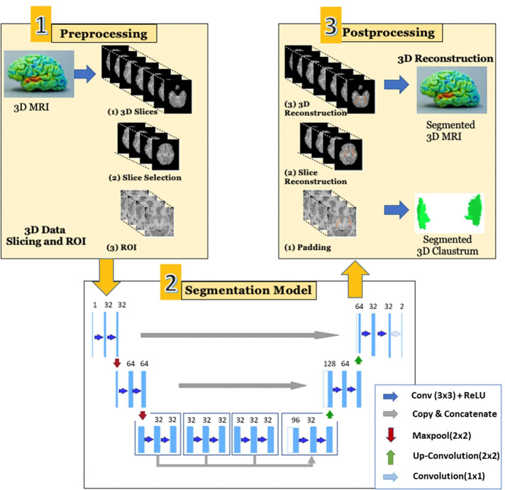
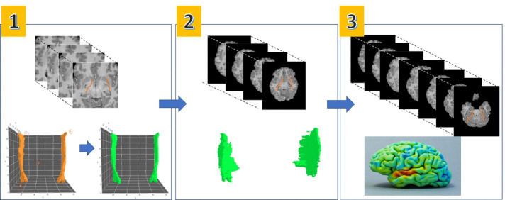
AM-UNet is a fully automated 3D segmentation network that is based on a 2D U-Net model. AM-UNet consists of three parts, preprocessing, segmentation, and postprocessing, as seen in Fig. 2. In the preprocessing step, the 3D MRI volumes are converted into a series of 2D slices, and the region of interests (ROIs) are created. The segmentation model is designed to segment a series of 2D ROIs based on 2D U-Net models. The postprocessing step reconstructs 3D MRI from the 2D segmented slices.
Fig. 2.
AM-UNet Architecture
Manual segmented human brain data
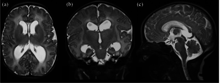
For this project, we used the MRI data of 30 healthy adults (13 males and 17 females; age range 21-35 years old) for CL segmentation. The dataset, including T1- and T2-weighted MRIs, were collected as a part of the Washington University-Minnesota Consortium Human Connectome Project (WU-Minn HCP) [46], which are available from the ConnectomDB [11]. The MRIs were acquired using a customized Siemens 3T Connectome Skyra scanner with the 3D MPRAGE T1 and T2 weighted sequence with 0.7 mm isotropic resolution (FOV=224 mm, matrix=320, 256 Sagittal slices in a single slab, TR=2400 ms, TE=2.14 ms, TI=1000 ms, flip angle=8). MRI scans can be viewed in the three orientational planes, Axial, Coronal, Sagittal as shown in Fig. 3. The details of MRI data collection and preprocessing methods are described in [50]. Using this dataset, we created T1T2 combined MRI (T1T2w) by integrating T1w and T2w images to improve the contrast between the gray and white matters [37] using the following formula:
| 1 |
Fig. 3.
Three Views of MRI Scans (from left to right) (a) Axial, (b) Coronal, (c) Sagittal
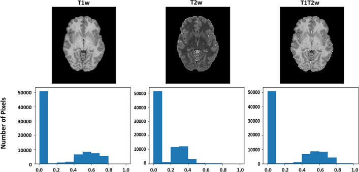
In Eq. 1, sT2 is a scaled T2 with the same median signal intensity (of brain part) as that of the T1 MRI. The combined MRI is further scaled to have the same median value as the original T1. Thus, T1T2w MRI has better grey/white matter contrasts, and due to the opposite directional signals of T1 and T2 and the calculations, the new MRI data has some high values in the brain’s margin. Figure 4 shows the T1w, T2w, and T1T2w MRI images along with graphs of their respective pixel intensities (normalized). As seen from this figure, the data has a class imbalance issue, and the majority of the pixels (50000) have 0.0 intensity (black background color). In [27], we reported the manual CL segmentation for the 30 T1 & T2 MRI scans based on a protocol developed for the conventional 3T resolution (1.0 mm isotropic voxels). This protocol is widely used for MRI-based human brain atlas [16]. The annotated CL label map in Nifti 3D format was used for the CL automatic segmentation.
Fig. 4.
T1w, T2w, and T1T2w MRIs and Normalized Pixel Intensities Graph
Preprocessing
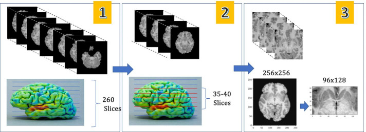
The preprocessing stage was designed to prepare the MRI data for the CL segmentation, as shown in Fig. 5. It was composed of three sub-stages: (1) processing of the 3D MRI slicing for the 2D U-Net segmentation (selection of 2D CL slices from 3D MRI), (2) processing of ROI selection from the 2D selected slices (ROI operation from 2D selected slices to 2D ROI images), and (3) machine learning techniques (data normalization and augmentation). Also, note that the preprocessing steps were performed for the multi-view CL segmentation of the axial, coronal, and sagittal planes.
Fig. 5.
Preprocessing for CL Segmentation: (1) 3D MRI Slicing (2) Slice Selection (3) ROI
The goal of the preprocessing step was to convert the 3D MRIs into 2D slices to generate ROIs, which will be used as an input by the 2D segmentation model. Initially, 2D slices were generated from 3D MR images to preprocess the data in a slice-wise fashion for optimal model performance, as shown in Fig. 5a. Each MRI contains around 260 slices for each subject. Therefore, all the input slices were resized to have the same pixel size of 256256. Secondly, the selection task was performed to ensure that only the slices containing CL were included in training the CL segmentation model. This step reduced the number of slices on average from 260 to 36 for each MRI, as shown in Fig. 5b. Lastly, we processed to overcome the issue of a massive class imbalance between the target (CL is approximately 0.3%) and the extensive background regions, which is shown in the intensities graphs of the three data types (T1w, T2w, and T1T2w; Fig. 4). To this end, the filtered slices were superimposed onto the region of interest (ROI) with a size of 96128 from the full-size slice with a size of 256256, as shown in Fig. 5c. After applying the ROI, each slice contained approximately 98.4% of background pixels and 1.6% of the CL pixels. Table 1 compares the number of CL and the background pixels before and after the ROI procedure. The ROI procedure significantly reduced the number of background pixels without affecting the number of the CL pixels, therefore decreasing the class imbalance.
Table 1.
The number of CL and the background pixels before and after an ROI procedure for three slices. The number of the CL pixels did not change before ROI () and after ROI (), but the number of background pixels is reduced significantly after the ROI procedure
| Slice | CL Size | Background Pixel# | |||
|---|---|---|---|---|---|
| ID | Pixel# | Ratio() | Ratio() | Before ROI | After ROI |
| 1 | 198 | 0.3% | 1.6% | 65338 | 12090 |
| 2 | 209 | 0.3% | 1.7% | 65327 | 12079 |
| 3 | 187 | 0.28% | 1.5% | 65349 | 12101 |
Besides the preprocessing of MRI images, machine learning (ML) techniques were applied to increase the performance. In our study, normalization was performed on the ROI’s pixel intensities ranging from 0 to 1. Further, data was augmented to produce the desired invariance properties and increase the training dataset. Additional slices were synthetically generated using the stretching technique. With data augmentation, the size of training data was increased from 855 to 1069 slices, as shown in Table 2.
Table 2.
AM-UNet Dataset
| Subjects | MRI Slices | Selected Slices# | ROI+Aug. | |||||||
|---|---|---|---|---|---|---|---|---|---|---|
| Num. | M/F | Age | Slice | Size | Min | Avg | Max | Total | Size | Total |
| 30 | 13/17 | 21-35 | 260 | 256x256 | 21 | 36 | 47 | 855 | 96x128 | 1069 |
CL segmentation model architecture
In our previous work [3], we designed a U-Net architecture for human brain CL segmentation and obtained an average dice score of 72%. This U-Net architecture consists of an encoder and a decoder, which performed downsampling and upsampling with four layers, and are connected through skip connections for the construction of a high-resolution image. The proposed optimal U-Net architecture of AM-UNet, shown in Fig. 2, is an extension of our previous architecture, making the model more simple and more efficient. In AM-UNet, we have reduced the segmentation model size to half by removing the last two layers of the original U-Net model and expanding the bottleneck layer of the segmentation model (Fig. 2). AM-UNet consists of an encoder and a decoder connected with skip connections. On the left, the encoder path is called the contracting path, and it captures the context from the images in a Nifti format T1w, T2w, or T1T2w MRI file. On the right, the decoder path is called the expanding path, and it enables the precise localization of the target (i.e., CL) that needs to be segmented.
The features learned at each level in the encoder path are transferred to the decoder path through skip connections, where the features from the encorder path will be concatenated with the features from the decoder path [41]. The encoder path maps a given input signal ’a’ that belongs to a set of signals ’A,’ which is a subset of all the signals ’R’ in the layer with the total number of dimensions ’d’, , to a feature space ’s’, which belongs to a set of feature spaces ’S,’ , and the decoder does the opposite of what the encoder does - taking the feature map as an input, processing it, and producing an output . The encoder and decoder paths are symmetric, and both have the same number of layers, say L. Eqs. 2 and 3 represent the input and output dimensions for the encoder layer, , and the decoder layer, , respectively, where represents the total dimension of the feature at the L-th layer.
| 2 |
| 3 |
As shown in Fig. 2 (Segmentation Model), the AM-UNet segmentation model consists of two layers along with the bottleneck layer, which is half of the size of the U-Net architecture. Each layer in the encoder path performs two rounds of convolution, batch normalization, and dropout, respectively. After that, the max-pooling reduces the image size by half and passes it to the next layer in the architecture. This process continues until the image reaches the last layer in the encoder path, called the bottleneck layer. We added three new blocks in this layer, each consisting of two rounds of convolution, batch normalization, and dropout, respectively. After the third block, we concatenated all the previous blocks’ output into the last block in the bottleneck layer. The three new block design was confirmed as optimal from the experiments with various numbers of blocks in the bottleneck layer.
The decoder path starts at the end of the bottleneck layer on the right side. Initially, upsampling is applied to increase the image resolution by a factor of 2. In regular upsampling, convolutions are replaced by transposed convolution to upsample the image. After that, the image is transferred to the next layer in the decoder path, which concatenates the feature maps from the contracting path (encoder), and performs two rounds of convolution, batch normalization, and dropout, respectively. After that image is upsampled again, the process continues until it reaches the last level in the decoder path, where image is restored to its original size of 96x128. The final layer in the decoder path has a sigmoid function that classifies each pixel in a binary way to a probability between 0 to 1.
We applied a window of 33 to the input image to construct a feature map in the convolution process. We used the ReLU activation function [21] in these convolution processes. This activation function did not change the features’ positive weights, but it assigned a value of zero to all the negative weights of the features. Batch normalization was used to accelerate the network training by reducing the rate at which each layer’s inputs distribution changes during training, as the previous layer’s parameters change [26]. To prevent overfitting, we implemented L2 and Dropout as regularization methods in the model. We also used early stopping [47] for the same reason. Adam optimizer was used to optimize the weight and bias at each layer in the network, with a learning rate of 0.001 [47]. The input to the model is an ROI image of a slice in a human brain MRI, and the output is the segmented CL image.
Compared to U-Net and UNet++, the AM-UNet architecture produces higher accurate results in less computation time on the CL dataset. It is half the size of U-Net and does not need the complex skip connections of UNet++. AM-UNet enables the model to produce quality segmentation results with a small amount of training data. Since we have removed the last two max-pooling layers from the original U-Net model, AM-UNet consumes fewer training parameters and is faster to converge. This model performs well for inter and intra-slice classification in detecting CL in identifying the coarse CL boundaries and segment them from the human brain MRI dataset.
Postprocessing
The postprocessing stage of the AM-UNet 3D segmentation network was designed to ensure a high prediction accuracy for 3D CL segmentation. It was composed of three sub-stages: (1) filtering false positives from the segmentation output, (2) reconstruction of the 2D slices from the segmented 2D ROIs (from 2D ROI images to 2D full images), (3) reconstruction of the 3D volumes from the 2D reconstructed slices (from 2D segmented slices to 3D MRI), as shown in Fig. 6. There was noise in the ground truth (manual annotation), which caused the segmentation model to falsely label some background pixels as CL. The false-positive removal step was designed to solve this issue. The removal of false positives was conducted through two steps: (i) each pixel was labeled with 1 or 0 that is 1 when probability (), and 0 otherwise; (ii) the false positive pixels in the non-CL region were further detected and removed. The non-CL region was determined considering the ROI (represented by a rectangular matrix of 96x128) of each slice. In this matrix, CL pixels were supposed to present in the left and right CL regions. Hence, we filtered out the pixels falling out of the regions.
Fig. 6.
Postprocessing for 3D MRI Reconstruction: (1) Filtering False Positives, (2) Reconstruction of 2D Slices, (3) Reconstruction of 3D MRI
Secondly, the 2D segmented slices, as shown in Fig. 6a, were restored to their original size of 256x256 using padding, as shown in Fig. 6b. Thus, each ROI (or image) at this stage is a slice of MRI. Finally, all the annotated slices for CL segmentation were stacked back to reconstruct each subject’s 3D MRI brain. Each subject MRI may have a different number of slices for CL segmentation. Thus, the 3D MRI brain was reconstructed by replacing the original slices with the annotated slices, as shown in Fig. 6c.
Loss function
The AM-Net model used the stochastic gradient descent optimization algorithm and evaluated the model’s performance using the loss function of Weighted Binary Cross-Entropy (WBCE) [24] during training. The higher value of the loss function indicates that the model is off, whereas the lower value indicates a good training performance. The WBCE loss function reduced the classification error due to the class imbalance between the target (CL) and the background pixels and resulted in the enhancement of the model performance. The WBCE is defined in Eq. 4.
| 4 |
Where M represents the number of the training examples, w is the weight, is the target label for the training example m, represents the input training example m, and is the model with neural network weight .
Results and evaluation
Dataset
We used the 30 subjects’ high-resolution HCP MRIs (0.7 mm isotropic voxels) that were manually traced by domain experts using the manual tracing protocol. The manual segmentation protocol [27] was developed using a cellular-level human brain atlas [15] that incorporated neuroimaging (T1 & diffusion-weighted MRI), high-resolution histology, large-format cellular resolution Nissl, and immunohistochemistry anatomical plates of an intact adult brain. T1w, T2w, and T1T2w MRI were used to produce segmentation maps for the Axial, Coronal, and Sagittal views (see Table 2 for the details of this dataset).
Evaluation metrics
To quantitatively evaluate the model accuracy, we have calculated various evaluation measures, including Dice score, Intersection over Union (IoU), Intraclass Correlation Coefficient (ICC), Sensitivity, Specificity, False Positive Rate (FPR), False Negative Rate (FNR), and Precision. True positive (TP) indicates the number of the CL pixels correctly predicted by the model. True negative (TN) indicates the number of the background pixels correctly predicted by the model. False positive (FP) indicates the number of background pixels that the model incorrectly predicted as CL. False negative (FN) indicates the number of CL pixels that the model incorrectly predicted as the background. Dice score is an index used to gauge the similarity of two samples in a range from 0 to 1 (see Eq. 5). The higher the value of the Dice score, the better is the accuracy of the model. IoU is an evaluation metric used to measure the accuracy of the image segmentation model by dividing the area of overlap between the predicted bounding box and the ground-truth bounding box by the total area encompassed by both, the predicted bounding box and the ground-truth bounding box, using Eq. 6.
| 5 |
| 6 |
For measuring the reliability of our evaluation, we used Intraclass Correlations (ICC), which describes how the observations in the same class resemble each other [42]. It is the index that reflects both degrees of correlation and agreement between measurements. In ICC3, each subject was assessed by each rater, but the raters were the only raters of interest, and the reliability was calculated from a single measurement, while ICC(3,K) was assessed by taking an average of the k raters’ measurement. Eq. 7 and 8 shows the formula for ICC3 and ICC(3,k) calculations respectively, where is the mean square for rows, is the mean square for residual sources of variance, is the mean square for error, represents mean square for columns, and K represents the number of raters/measurements.
| 7 |
| 8 |
We also computed the following measures: true positive rate (TPR) (Sensitivity) to determine how often our model can correctly identify the CL pixel (Eq. 9), true negative rate (TNR) (Specificity) to determine how often our model can correctly identify background pixels (Eq. 10), false positive rate (FPR) to determine how often the model incorrectly identifies background pixel as Cl (Eq. 11), False-negative rate (FNR) to measure how often the model will incorrectly identify CL pixel as background (Eq. 12), and Positive Predictive Value (PPV) (Precision) to measure how many pixels are CL out of all the pixels that the model has identified as CL for the CL segmentation (Eq. 13).
| 9 |
| 10 |
| 11 |
| 12 |
| 13 |
AM-UNet: slice and subject level performance
We calculated the evaluation metrics with k-fold cross-validation performed on the 30 subject MRI dataset. For CL segmentation, we evaluated AM-UNet performance on multiple MRIs, including T1w, T2w, and T1T2w, with three different views, including Axial, Coronal, and Sagittal views. We conducted the evaluation of the model on each of the three datasets separately, and for each run, we used k-fold cross-validation with the value of k = 5. The dataset was divided into five equal parts during each run. The model was trained on four parts and tested on one part. Then, the values of the evaluation parameters were recorded. This process was repeated five times so that model was tested on the whole dataset, and the average values for evaluation parameters were obtained at the end.
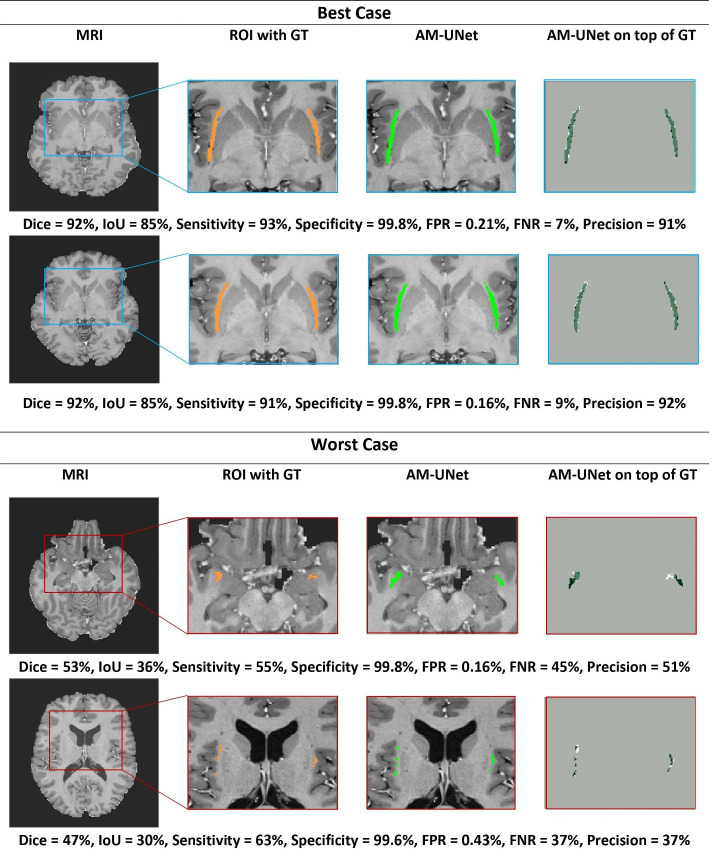
We trained the model on the augmented dataset for CL segmentation and tested it on a non-augmented one. With this procedure, we obtained an average Dice score of 82%, 81%, and 82% and an average IoU score of 69%, 68%, and 70% for the CL segmentation for the Axial view of T1w, T2w, and T1T2w MRI, respectively. Table 3 shows the average Dice and IoU scores of AM-UNet on the three datasets for the Axial and Coronal views. The Sagittal results have been omitted due to its poor performance that does not provide meaningful results. To the best of our knowledge, these results are state-of-the-art for 3D human brain CL segmentation. ICC3 and ICC(3,K), whose manual tracer (raters) are the only raters of interest (3), are relevant to measure the reliability of the AM-UNet model. We evaluated the accuracy of the model’s CL segmentation, the single average measure of many pixels (K). Our model achieved 90% and 81% for ICC(3,K) and ICC3 respectively for T1T2w data set for the Axial view. The average values of Sensitivity, Specificity, FPR, FNR, and Precision of AM-UNet are shown in Table 4. We achieved excellent overall scores on T1T2w data for the Axial view, such as Sensitivity (TPR) of 84.8%, Specificity (TNR) of 99.7%, FPR of 0.332%, FNR of 15.2% and Precision of 78.1%. We also evaluated AM-UNet on the slice level. Since our model was tested on the whole dataset, the model performance on individual slices was recorded. We analyzed the best and worst-case slices of our model for the Axial view T1T2w data. The details are shown in Fig. 7.
Table 3.
AM-UNet performance on T1w only, T2w only, and T1T2w data
| Axial view | Coronal view | |||
|---|---|---|---|---|
| Type | Dice Score(%) | IoU Score(%) | Dice Score(%) | IoU Score(%) |
| T1w | 82 | 69 | 81 | 68 |
| T2w | 81 | 68 | 81 | 68 |
| T1T2w | 82 | 70 | 82 | 70 |
| Number of Subjects = 30 | ||||
Table 4.
AM-UNet accuracy analysis for T1T2w MRI in axial view
| Metric | Average Value |
|---|---|
| Sensitivity (TPR) | 84.8% |
| Specificity (TNR) | 99.7% |
| False Positive Rate (FPR) | 0.332% |
| False Negative Rate (FNR) | 15.2% |
| Precision | 78.1% |
Fig. 7.
Best and worst cases of AM-UNet
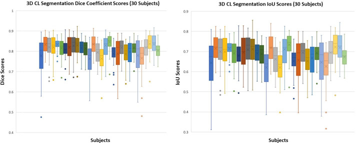
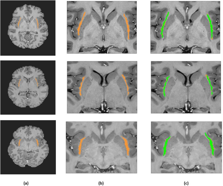
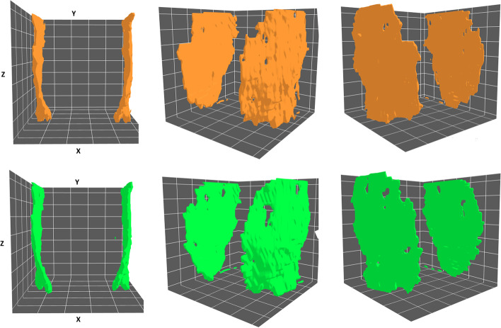
In addition, we evaluated AM-UNet performance on the subject level. As mentioned earlier, in the CL MRI dataset, each subject had 260 slices. Only slices containing CL (36 per subject on average) are presented to the segmentation model for prediction. Since we used the K-fold cross-validation approach for evaluation purposes, AM-UNet was tested on the whole dataset. The average Dice and IoU scores were calculated for the entire dataset. Figure 8 shows the boxplots for Dice and IoU per case score for all the 30 subjects in the dataset. Figure 9 depicts the ground truth (GT) and the model segmentation results of three subjects; the segmentation models precisely assigned each pixel of an image to one of the two classes, CL and the background. Figure 10 shows the 3D reconstructed volumes of GT and AM-UNet predictions.
Fig. 8.
Subject-wise Evaluation for 3D CL Segmentation: Dice Coefficient Scores (on left), IoU Scores (on right)
Fig. 9.
AM-UNet for CL Segmentation for 3 subjects: (a) Ground Truth, (b) Ground Truth (CL ROI), (c) Predicted Outcome
Fig. 10.
AM-UNet 3D Segmentation (Green) and Ground Truth (Orange)
Comparative evaluation
One of the closely related approaches to our work uses a fully convolutional network with a multi-view method [32]. This work employs a deep learning-based multi-view approach to segment CL from T1w data. Table 5 compares the Dice score accuracy of our model with the multi-view model. As seen in Table 5, the multi-view model [32] used 181 T1w MRI scans for training. As per the results in Table 5, with only 30 MRIs as training data, our model has shown better performance in all three views. The multi-view model [32] also generated segmentation maps for Axial + Coronal and Axial + Coronal + Sagittal views and obtained the Dice score of 0.718 and 0.710, respectively. AM-UNet achieved better performance in all these three views even with less data, as seen in Table 5. Thus, we have not generated segmentation maps for Axial + Coronal and Axial + Coronal + Sagittal views that can be our future work.
Table 5.
Comparative evaluation: AM-UNet & multi-view CL model
| Model | Dice score | Subject | ||
|---|---|---|---|---|
| Axial | Coronal | Sagittal | ||
| Multi-View Convol. Network (T1 Only) [32] | 0.69 | 0.70 | 0.55 | 181 |
| AM-UNet (T1 Only) | 0.82 | 0.81 | 0.68 | 30 |
| AM-UNet (T1T2) | 0.82 | 0.82 | 0.68 | |
Furthermore, AM-UNet was compared with the CL segmentation implementation using U-Net [41] and UNet++ [41]. Both of these models have shown promising results in the image segmentation domain. The CL segmentation models based on U-Net and UNet++ were trained in our experiment setting. Table 6 shows the results of this experiment for the Axial view using K-fold cross-validation with the value of k equal to 5. We computed the Dice and IoU scores for all three datasets (T1w, T2w, and T1T2w) but only reported the scores for T1T2w data.
Table 6.
Comparative evaluation: AM-UNet & state-of-the-Art UNet networks
| Model | Average dice score | Average IoU | ICC | |||||
|---|---|---|---|---|---|---|---|---|
| T1 | T2 | T1T2 | T1 | T2 | T1T2 | ICC3 | ICC(3,K) | |
| U-Net [41] | 0.81 | 0.78 | 0.81 | 0.68 | 0.64 | 0.69 | 0.78 | 0.87 |
| UNet++ [41] | 0.80 | 0.80 | 0.81 | 0.67 | 0.69 | 0.68 | 0.7 | 0.87 |
| AM-UNet | 0.82 | 0.81 | 0.82 | 0.69 | 0.68 | 0.70 | 0.81 | 0.90 |
| Model | TPR | TNR | FPR | FNR | Prec | #Par | ||
| U-Net [41] | 0.80 | 0.996 | 0.0036 | 0.76 | 0.20 | 8.6M | ||
| UNet++ [1] | 0.78 | 0.998 | 0.0024 | 0.22 | 0.82 | 9M | ||
| AM-UNet | 0.85 | 0.997 | 0.0033 | 0.15 | 0.78 | 0.34M | ||
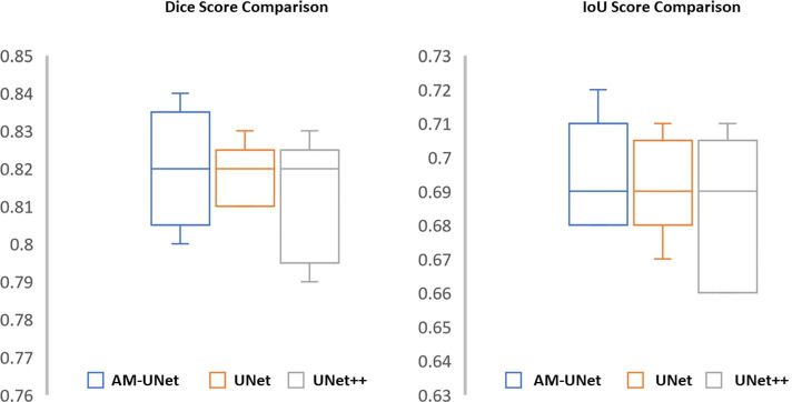
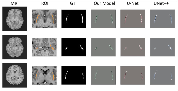
As seen in Table 6, AM-UNet has shown better results in most evaluation indicators. It has outperformed U-Net and UNet++ in the six metrics out of the nine ones. AM-UNet has achieved the best results for most of the critical evaluation parameters for the CL segmentation. Our method obtained the best scores for five evaluation metrics (Dice, IoU, ICC, TPR, FNR) and has used significantly fewer training parameters(#Par). Our method’s higher TPR score and lower FNR score verify that AM-UNet is optimized in detecting the CL pixels. UNet++ has achieved the best scores of three scores (TNR, precision, and FPR). UNet++ had the highest precision score because it predicted only a few CL pixels with high accuracy (and hence missed some CL pixels), and therefore it obtained a low FPR score. The high TNR of UNet++ shows its ability to identify the background pixels correctly. The U-Net model received poor results, such as the lowest precision and the highest score of FNR and FPR. The boxplots comparing the Dice and IoU scores across these three methods, Fig. 11, confirms the results presented in Table 6. Figure 12 shows the visual comparison of the three models on the T1T2w dataset for the Axial view. In this figure, MRI represents the input data, ROI represents the region of interest with CL highlighted in orange, GT represents the ground truth labels in white, AM-UNet represents the result of our model in green overlaid on white ground truth, U-Net represents the results of U-Net in red overlaid on white ground truth, and UNet++ represents the results of UNet++ in blue overlaid on white ground truth. The overlaid regions’ darker green, red, or blue pixels mean false positives, and white pixels represent false negatives. As seen in Fig. 12, U-Net and UNet++ had high false negative rates and lower true positive rates and therefore has more white pixels as compared to AM-UNet. In terms of false positive rates (the darker pixels), all the three models showed similar results, with UNet++ having marginally better performance than others.
Fig. 11.
Evaluation with Dice Score & IoU Score: AM-UNet, U-Net, and UNet++
Fig. 12.
Comparative Evaluation: Original and ROI Images, Ground Truth (white), AM-UNet (Green), U-Net (Red), and UNet++ (Blue)
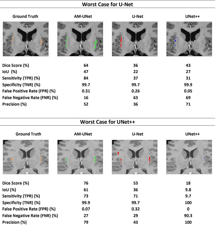
The performance of U-Net and UNet++ was also evaluated on individual MRI levels. In this evaluation, we identified the worst-cases of these two models, U-Net and UNet++, and compared the performance of all the three models, AM-UNet, U-Net, and UNet++, for these 2 MRIs. Figure 13 shows the result of this comparison. This figure presents the visual comparison for the model performance and the values for the seven evaluation measures. As seen in Fig. 13, our model outperformed the other two models in terms of Dice score, IoU, Sensitivity, and FNR for both the MRIs. UNet++ had better results for Precision and FPR, mainly because the model has missed a lot of the CL pixels. This is also evident from the high FNR and low TPR of UNet++ and the visuals provided in Fig. 13. As seen in the figure, UNet++ can barely identify the CL pixels in its worst-case and completely misses the right half of the CL on the worst-case for U-Net. Similarly, U-Net suffers from high FNR, and low TPR for its worst-case completely misses the suitable CL pixels and shows higher FPR for the worst-case for UNet++.
Fig. 13.
Comparative Analysis with Worst Cases of U-Net and UNet++
Discussion
First, 3D segmentation modeling requires more complex modeling and much higher computational resources [1], which in turn affects a modeling ability to carry out the training with large datasets. Some studies reported that 2D U-Net achieved better results than 3D U-Net’s in terms of accuracy, memory consumption, and training time [33]. Targeting the 3D segmentation in AM-UNet, a series of multiple 2D segmentation models were designed instead of a 3D segmentation model. In AM-UNet, we utilized advanced pre and postprocessing image analysis techniques and the 2D segmentation model to create a fully automated end-to-end 3D segmentation network. As a result, we obtained a superior performance from AM-UNet compared to others. Our study showed that the simplicity of the AM-UNet model is sufficient to capture the spatial information along the third dimension, like 3D models. Furthermore, AM-UNet also can represent the 3D CL segmentation with a series of 2D segmentation models.
Second, compared to other subcortical brain structures that are often segmented manually (e.g., amygdala), CL is much harder to segment accurately due to the thin morphology and the limited spatial resolutions of MR images. In this study, our AM-UNet approach with optimized image analysis strategies solves the challenging problem of segmenting CL. The comparative evaluation demonstrates the AM-UNet’s ability for the CL segmentation. The results obtained in this research and the comparison with other works have shown the AM-UNet’s strengths. To the best of our knowledge, we achieved the state of the art results for automatic end-to-end 3D CL segmentation. The present study demonstrated that our AM-UNet approach has great potential for developing an automatic and accurate segmentation tool for very challenging medical imaging segmentation problems, such as CL segmentation.
Finally, there is still room to improve the AM-UNet model: We need an advanced method to overcome a challenging problem of the CL segmentation, such as the class imbalance problem (i.e., background pixels vs. CL pixels). We need more powerful ROI detection dealing with diverse MRI datasets. The deep learning networks could be extended for capturing contextual features of CL with advanced models, such as attention modeling or sequential modeling with LSTM. We need to consider a semi-supervised approach for CL segmentation through human and machine collaboration to overcome the lack of human-annotated data rather than supervised learning.
Conclusion and future work
We proposed AM-UNet for CL segmentation of the human brain MRIs, consisting of preprocessing, optimal U-Net-based modeling, and postprocessing. AM-UNet produced the 3D CL segmentation maps for human brain MRIs effectively and efficiently. We developed and evaluated various deep learning models (U-Net variants) to automatically and accurately segment the CL from T1, T2, and T1T2 weighted MRI datasets. Among these models, we found that AM-UNet had the optimal performance and simplified architecture for 3D MRI segmentation. Our main contributions of this research are as follows: (i) designed a smaller, simpler, and efficient U-Net model architecture, (ii) developed an automated end-to-end 3D segmentation network for CL, (iii) produced multi-view segmentation models, and (iv) obtained the state-of-the-art results in the 3D CL segmentation. For automatic segmentation of 30 human brain MRIs (T1T2w) from the HCP dataset, the AM-UNet network has achieved superior segmentation performance with Dice, IoU, and ICC scores for the Axial view’s CL segmentation of 82%, 70%, and 90%, respectively. The 2D segmentation version of AM-UNet is publicly available on GitHub: https://github.com/AhmedAlbishri/AM-UNET.
In future work, we will enhance the AM-UNet approach for a 3D U-Net-based CL segmentation model. As a result, the segmentation model will be more flexible with various imaging datasets in a wide range of medical applications. Furthermore, the model will be extended to use segmentation maps for Axial + Coronal and Axial + Coronal + Sagittal views. We will also develop an interactive 3D segmentation tool for MRI and CT-Scan images in which experts can give immediate feedback during machine learning and pre/post-processing. In addition, this tool will provide advanced features, such as normalization, augmentation, transformation, visualization, optimization, and transfer learning for effective CL segmentation.
Acknowledgements
This work was partially supported by NSF CNS #1747751 awarded to Lee and NASARD Young Investigator Grant 25158 awarded to Kang. We appreciate Joseph Bodenheimer for his help with the MRI data used in the current study.
Footnotes
Ahmed Awad Albishri and Syed Jawad Hussain Shah have contributed equally to this work.
Publisher’s Note
Springer Nature remains neutral with regard to jurisdictional claims in published maps and institutional affiliations.
Contributor Information
Ahmed Awad Albishri, Email: aa8w2@umsystem.edu, Email: a.albishri@seu.edu.sa.
Syed Jawad Hussain Shah, Email: shs6g7@umsystem.edu.
Seung Suk Kang, Email: kangseung@umkc.edu.
Yugyung Lee, Email: leeyu@umkc.edu.
References
- 1.Alalwan N, Abozeid A, ElHabshy AA, Alzahrani A. Efficient 3d deep learning modelfor medical image semantic segmentation. Alex Eng J. 2021;60(1):1231–1239. doi: 10.1016/j.aej.2020.10.046. [DOI] [Google Scholar]
- 2.Albishri A, Shah SJ, Lee Y (2019) Cu-net: cascaded u-net model for automated liver and lesion segmentation and summarization. In: 2019 IEEE international conference on bioinformatics and biomedicine (IEEE BIBM 2019)
- 3.Albishri AA, Shah SJH, Schmiedler A, Kang SS, Lee Y (2019) Automated human claustrum segmentation using deep learning technologies. arXiv preprint arXiv:1911.07515
- 4.Asperti A, Mastronardo C (2017) The effectiveness of data augmentation for detection of gastrointestinal diseases from endoscopical images. arXiv preprint arXiv:1712.03689
- 5.Badrinarayanan V, Kendall A, Cipolla R. Segnet: a deep convolutional encoder-decoder architecture for image segmentation. IEEE Trans Pattern Anal Machine Intell. 2017;39(12):2481–2495. doi: 10.1109/TPAMI.2016.2644615. [DOI] [PubMed] [Google Scholar]
- 6.Bae HJ, Hyun H, Byeon Y, Shin K, Cho Y, Song YJ, Yi S, Kuh SU, Yeom JS, Kim N. Fully automated 3d segmentation and separation of multiple cervical vertebrae in ct images using a 2d convolutional neural network. Comput Methods Programs Biomed. 2020;184:105119. doi: 10.1016/j.cmpb.2019.105119. [DOI] [PubMed] [Google Scholar]
- 7.Benjelloun M, Mahmoudi S. Spine localization in x-ray images using interest point detection. J Digital Imaging. 2009;22(3):309–318. doi: 10.1007/s10278-007-9099-3. [DOI] [PMC free article] [PubMed] [Google Scholar]
- 8.Bernstein HG, Ortmann A, Dobrowolny H, Steiner J, Brisch R, Gos T, Bogerts B. Bilaterally reduced claustral volumes in schizophrenia and major depressive disorder: a morphometric postmortem study. European Archives of Psychiatry and Clinical Neuroscience. 2016;266(1):25–33. doi: 10.1007/s00406-015-0597-x. [DOI] [PubMed] [Google Scholar]
- 9.Castro E, Cardoso JS, Pereira JC (2018) Elastic deformations for data augmentation in breast cancer mass detection. In: 2018 IEEE EMBS international conference on biomedical & health informatics (BHI). IEEE, pp 230–234
- 10.Christ PF, Ettlinger F, Grün F, Elshaera MEA, Lipkova J, Schlecht S, Ahmaddy F, Tatavarty S, Bickel M, Bilic P, et al (2017) Automatic liver and tumor segmentation of ct and mri volumes using cascaded fully convolutional neural networks. arXiv preprint arXiv:1702.05970
- 11.Connectomdb. https://db.humanconnectome.org/. [Online; Accessed 17 Nov 2019]
- 12.Crick FC, Koch C. What is the function of the claustrum? Philosophical Transactions of the Royal Society B: Biological Sciences. 2005;360(1458):1271–1279. doi: 10.1098/rstb.2005.1661. [DOI] [PMC free article] [PubMed] [Google Scholar]
- 13.Cruz-Roa AA, Ovalle JEA, Madabhushi A, Osorio FAG (2013) A deep learning architecture for image representation, visual interpretability and automated basal-cell carcinoma cancer detection. In: International conference on medical image computing and computer-assisted intervention. Springer, pp 403–410 [DOI] [PubMed]
- 14.Davis WB (2008) The claustrum in autism and typically developing male children: A quanti-tative mri study. Brigham Young University-Provo
- 15.Ding SL, Royall JJ, Sunkin SM, Ng L, Facer BA, Lesnar P, Guillozet-Bongaarts A, McMurray B, Szafer A, Dolbeare TA, et al. Comprehensive cellular-resolution atlas of the adult human brain. Journal of Comparative Neurology. 2016;524(16):3127–3481. doi: 10.1002/cne.24080. [DOI] [PMC free article] [PubMed] [Google Scholar]
- 16.Ding SL, Royall JJ, Sunkin SM, Ng L, Facer BA, Lesnar P, Guillozet-Bongaarts A, McMurray B, Szafer A, Dolbeare TA, et al. Comprehensive cellular-resolution atlas of the adult human brain. The Journal of Comparative Neurology. 2017;525(2):407. doi: 10.1002/cne.24130. [DOI] [PMC free article] [PubMed] [Google Scholar]
- 17.Dou Q, Yu L, Chen H, Jin Y, Yang X, Qin J, Heng PA. 3d deeply supervised network for automated segmentation of volumetric medical images. Medical Image Analysis. 2017;41:40–54. doi: 10.1016/j.media.2017.05.001. [DOI] [PubMed] [Google Scholar]
- 18.Duncan JS, Ayache N. Medical image analysis: progress over two decades and the challenges ahead. IEEE Trans Pattern Anal Machine Intell. 2000;22(1):85–106. doi: 10.1109/34.824822. [DOI] [Google Scholar]
- 19.Fan DP, Zhou T, Ji GP, Zhou Y, Chen G, Fu H, Shen J, Shao L. Inf-net: automatic covid-19 lung infection segmentation from ct images. IEEE Trans Med Imaging. 2020;39(8):2626–2637. doi: 10.1109/TMI.2020.2996645. [DOI] [PubMed] [Google Scholar]
- 20.Fischl B (2012) Freesurfer. Neuroimage 62(2):774–781 [DOI] [PMC free article] [PubMed]
- 21.Glorot X, Bordes A, Bengio Y (2011) Deep sparse rectifier neural networks. In: Proceedings of the fourteenth international conference on artificial intelligence and statistics, pp 315–323
- 22.Goll Y, Atlan G, Citri A. Attention: the claustrum. Trends in Neurosciences. 2015;38(8):486–495. doi: 10.1016/j.tins.2015.05.006. [DOI] [PubMed] [Google Scholar]
- 23.Havaei M, Davy A, Warde-Farley D, Biard A, Courville A, Bengio Y, Pal C, Jodoin PM, Larochelle H. Brain tumor segmentation with deep neural networks. Medical Image Analysis. 2017;35:18–31. doi: 10.1016/j.media.2016.05.004. [DOI] [PubMed] [Google Scholar]
- 24.Ho Y, Wookey S. The real-world-weight cross-entropy loss function: modeling the costs of mislabeling. IEEE Access. 2019;8:4806–4813. doi: 10.1109/ACCESS.2019.2962617. [DOI] [Google Scholar]
- 25.Huang H, Lin L, Tong R, Hu H, Zhang Q, Iwamoto Y, Han X, Chen YW, Wu J (2020) Unet 3+: a full-scale connected unet for medical image segmentation. In: ICASSP 2020-2020 IEEE international conference on acoustics, speech and signal processing (ICASSP). IEEE, pp 1055–1059
- 26.Ioffe S, Szegedy C (2015) Batch normalization: accelerating deep network training by reducing internal covariate shift. arXiv preprint arXiv:1502.03167
- 27.Kang SS, Bodenheimer J, Butler T (2020) A comprehensive protocol for manual segmentation of the human claustrum and its sub-regions using high-resolution mri. arXiv preprint arXiv:2010.06423
- 28.Kayalibay B, Jensen G, van der Smagt P (2017) Cnn-based segmentation of medical imaging data. arXiv preprint arXiv:1701.03056
- 29.Kushibar K, Valverde S, González-Villà S, Bernal J, Cabezas M, Oliver A, Lladó X (2017) Automated sub-cortical brain structure segmentation combining spatial and deep convolutional features. arXiv preprint arXiv:1709.09075 [DOI] [PubMed]
- 30.Larobina M, Murino L. Medical image file formats. Journal of Digital Imaging. 2014;27(2):200–206. doi: 10.1007/s10278-013-9657-9. [DOI] [PMC free article] [PubMed] [Google Scholar]
- 31.LeCun Y, Bengio Y, Hinton G, Scholar Google. Deep learning. Nature. 2015;521(7553):436. doi: 10.1038/nature14539. [DOI] [PubMed] [Google Scholar]
- 32.Li H, Menegaux A, Shit S, Schmitz-Koep B, Sorg C, Menze B, Hedderich D, et al (2020) Complex grey matter structure segmentation in brains via deep learning: example of the claustrum. arXiv preprint arXiv:2008.03465
- 33.Li X, Chen H, Qi X, Dou Q, Fu CW, Heng PA. H-denseunet: hybrid densely connected unet for liver and tumor segmentation from ct volumes. IEEE Transactions on Medical Imaging. 2018;37(12):2663–2674. doi: 10.1109/TMI.2018.2845918. [DOI] [PubMed] [Google Scholar]
- 34.Long J, Shelhamer E, Darrell T (2015) Fully convolutional networks for semantic segmentation. In: Proceedings of the IEEE conference on computer vision and pattern recognition, pp 3431–3440 [DOI] [PubMed]
- 35.Mathur BN. The claustrum in review. Frontiers in Systems Neuroscience. 2014;8:48. doi: 10.3389/fnsys.2014.00048. [DOI] [PMC free article] [PubMed] [Google Scholar]
- 36.Meletti S, Slonkova J, Mareckova I, Monti G, Specchio N, Hon P, Giovannini G, Marcian V, Chiari A, Krupa P, et al. Claustrum damage and refractory status epilepticus following febrile illness. Neurology. 2015;85(14):1224–1232. doi: 10.1212/WNL.0000000000001996. [DOI] [PMC free article] [PubMed] [Google Scholar]
- 37.Misaki M, Savitz J, Zotev V, Phillips R, Yuan H, Young KD, Drevets WC, Bodurka J. Contrast enhancement by combining t 1-and t 2-weighted structural brain mr images. Magnetic Resonance in Medicine. 2015;74(6):1609–1620. doi: 10.1002/mrm.25560. [DOI] [PMC free article] [PubMed] [Google Scholar]
- 38.Moeskops P, Viergever MA, Mendrik AM, de Vries LS, Benders MJ, Išgum I. Automatic segmentation of mr brain images with a convolutional neural network. IEEE Transactions on Medical Imaging. 2016;35(5):1252–1261. doi: 10.1109/TMI.2016.2548501. [DOI] [PubMed] [Google Scholar]
- 39.Mohamad IB, Usman D. Standardization and its effects on k-means clustering algorithm. Research Journal of Applied Sciences, Engineering and Technology. 2013;6(17):3299–3303. doi: 10.19026/rjaset.6.3638. [DOI] [Google Scholar]
- 40.Ren S, He K, Girshick R, Sun J (2015) Faster r-cnn: towards real-time object detection with region proposal networks. In: Advances in neural information processing systems, pp 91–99 [DOI] [PubMed]
- 41.Ronneberger O, Fischer P, Brox T (2015) U-net: convolutional networks for biomedical image segmentation. In: International conference on medical image computing and computer-assisted intervention. Springer, pp 234–241
- 42.Shrout PE, Fleiss JL. Intraclass correlations: uses in assessing rater reliability. Psychological Bulletin. 1979;86(2):420. doi: 10.1037/0033-2909.86.2.420. [DOI] [PubMed] [Google Scholar]
- 43.Silva G, Jacob S, Melo C, Alves D, Costa D. Claustrum sign in a child with refractory status epilepticus after febrile illness: why does it happen? Acta Neurologica Belgica. 2018;118(2):303–305. doi: 10.1007/s13760-017-0820-9. [DOI] [PubMed] [Google Scholar]
- 44. Smythies JR, Edelstein LR, Ramachandran VS (2014) Hypotheses relating to the functionof the claustrum. In: The Claustrum, pp 299–352. Elsevier
- 45.Torgerson CM, Irimia A, Goh SM, Van Horn JD. The dti connectivity of the human claustrum. Human Brain Mapping. 2015;36(3):827–838. doi: 10.1002/hbm.22667. [DOI] [PMC free article] [PubMed] [Google Scholar]
- 46.Van Essen DC, Smith SM, Barch DM, Behrens TE, Yacoub E, Ugurbil K, Consortium WMH, et al. The wu-minn human connectome project: an overview. Neuroimage. 2013;80:62–79. doi: 10.1016/j.neuroimage.2013.05.041. [DOI] [PMC free article] [PubMed] [Google Scholar]
- 47.Wan L, Zeiler M, Zhang S, Le Cun Y, Fergus R (2013) Regularization of neural networks using dropconnect. In: International conference on machine learning, pp 1058–1066
- 48.Wegiel J, Flory M, Kuchna I, Nowicki K, Ma SY, Imaki H, Wegiel J, Frackowiak J, Kolecka BM, Wierzba-Bobrowicz T, et al. Neuronal nucleus and cytoplasm volume deficit in children with autism and volume increase in adolescents and adults. Acta Neuropathologica Communications. 2015;3(1):2. doi: 10.1186/s40478-015-0183-5. [DOI] [PMC free article] [PubMed] [Google Scholar]
- 49.Woo CW, Chang LJ, Lindquist MA, Wager TD. Building better biomarkers: brain models in translational neuroimaging. Nature Neuroscience. 2017;20(3):365. doi: 10.1038/nn.4478. [DOI] [PMC free article] [PubMed] [Google Scholar]
- 50.WU-Minn H (2017) 1200 subjects data release reference manual. https://www.humanconnectome.org
- 51.Yamanakkanavar N, Choi JY, Lee B. Mri segmentation and classification of human brain using deep learning for diagnosis of alzheimer’s disease: a survey. Sensors. 2020;20(11):3243. doi: 10.3390/s20113243. [DOI] [PMC free article] [PubMed] [Google Scholar]
- 52.Zhou Z, Siddiquee MMR, Tajbakhsh N, Liang J. Unet++: redesigning skip connections to exploit multiscale features in image segmentation. IEEE Transactions on Medical Imaging. 2019;39(6):1856–1867. doi: 10.1109/TMI.2019.2959609. [DOI] [PMC free article] [PubMed] [Google Scholar]
- 53.Zhu H (2003) Medical image processing overview. University of Calgary, pp 1–27


