

Abstract
Recent advances in computer vision and machine learning underpin a collection of algorithms with an impressive ability to decipher the content of images. These deep learning algorithms are being applied to biological images and are transforming the analysis and interpretation of imaging data. These advances are positioned to render difficult analyses routine and to enable researchers to carry out new, previously impossible experiments. Here we review the intersection between deep learning and cellular image analysis and provide an overview of both the mathematical mechanics and the programming frameworks of deep learning that are pertinent to life scientists. We survey the field’s progress in four key applications: image classification, image segmentation, object tracking, and augmented microscopy. Last, we relay our labs’ experience with three key aspects of implementing deep learning in the laboratory: annotating training data, selecting and training a range of neural network architectures, and deploying solutions. We also highlight existing datasets and implementations for each surveyed application.
Advances in imaging have transformed the biological sciences, enabling researchers to access temporal and spatial variations inherent in living systems. Progress in optics has yielded microscopes capable of imaging over a range of spatial scales, from single molecules to entire organisms. Concurrently, improvements in fluorescent probes have enhanced the brightness, photostability, and spectral range of fluorescent proteins and of small-molecule dyes. Combined, these advances allow for a variety of dynamic measurements in living cells, from long-term imaging of single molecules1,2, to simultaneous measurements of multiple biosensors3,4, to observations of the development of entire organisms5–9. They have also led to impressive measurements in fixed samples, with spatial genomics now driving the simultaneous measurement of dozens of proteins or thousands of mRNA species in fixed cells and tissues while preserving spatial information10–12.
Concurrent with these technological advances has been an increasing demand in the biosciences for image analysis. Modern imaging data increasingly require quantification to be informative13. Typical tasks include unsupervised image exploration (comparing features of collections of images, for example, by identifying changes in cellular morphology in an imaging-based drug screen), image classification (predicting a label for an image—for example, determining whether a stem cell has differentiated), image segmentation (identifying the parts of an image that correspond to distinct objects—for example, identifying single cells in images), and object tracking (following an object—for example, a single cell in a live embryo—among frames of a movie). In response to this demand, researchers and companies have developed software libraries, use-case-based implementations, and general-purpose computer vision ecosystems. MATLAB was one of the first commercial platforms to support solutions for computer vision and continues to enjoy frequent use. Recently, the development of open-source data-science libraries for Python (e.g., NumPy14, SciPy15, Pandas16, Scikit-image17, Scikit-learn18, Matplotlib19, and Jupyter20) has led to a rise in Python’s popularity. Both MATLAB and Python now contain ready-made implementations of common computer-vision algorithms. Traditionally, experimentalists wrote software tools that drew from these libraries. As analysis tasks became more common, several software tools were created to improve accessibility through a graphical front-end. For example, there are tools for single-cell analysis of bacteria (SuperSegger21, Oufti22, Morphometries23), single-cell analysis of mammalian cells (CellProfiler24,25, Ilastik26, Microscopy Image Browser27), and general-purpose image analysis (ImageJ28, OMERO29). These tools and ecosystems have transformed experimental design, rendered quantitative and statistical analyses automatable and high-throughput, and yielded a plethora of critical biological insights.
Excitingly, deep learning has expanded the range of problems that computer vision can solve30. Here, “deep learning” refers to a set of machine-learning techniques, specifically, neural networks that learn effective representations of data with multiple levels of abstraction30. Note the contrast with conventional machine learning, in which representations are manually designed through feature engineering. In deep learning, the learning can be supervised or unsupervised. Supervised approaches, which have been the most successful, attempt to maximize performance on an annotated dataset. Unsupervised approaches are used to reconstruct original data after compression into a low-dimensional space. Although these techniques have existed in mathematical form for several decades, they gained attention when a deep-learning-based method won the 2012 ImageNet Large Scale Visual Recognition Challenge31. Since then, there has been a major increase in the variety of problems that can be solved with deep learning. In addition, improvements in computer hardware and deep learning frameworks have placed these tools within reach of the typical software developer. While deep learning has been predominantly applied commercially, it is now starting to emerge in the physical32–34, chemical35,36, medical37,38, and biological sciences39–42 with applications for images and other data types.
Given the central role that observation—and therefore imaging—plays in the biological sciences, deep learning has the potential to revolutionize understanding of the inner workings of living systems. Indeed, currently a ‘gold rush’ is taking place, with numerous groups seeking to apply these methods to their data in order to extract novel biological insights. Nonetheless, deep learning has yet to be widely adopted throughout the life and medical sciences. Importantly, many of the software tools mentioned above (with the recent exceptions of CellProfiler25 and ImageJ43) do not yet feature deep learning. In our opinion, for deep learning to truly transform the life sciences, its application needs to be as routine as BLAST searches. The barriers to spreading deep learning throughout biology labs are both cultural and technical. The mathematics renders some of the inner workings of deep learning algorithms opaque; the unique requirements of deep learning necessitate a different way of thinking about writing software. Specifically, the need for annotated data means that data and software must be jointly developed—an approach recently termed Software 2.044 (Fig. 1). The amount of data and the computational resources required for deep learning constitute a significant barrier to adoption, as does the knowledge required to optimize model performance and to interpret what deep learning models have learned. To harness the full power of these tools, life scientists must familiarize themselves with them to enhance their existing workflows and to set the stage for currently unforeseen analyses.
Fig. 1 |. Software 2.0 combines data annotations with deep learning to produce intelligent software.
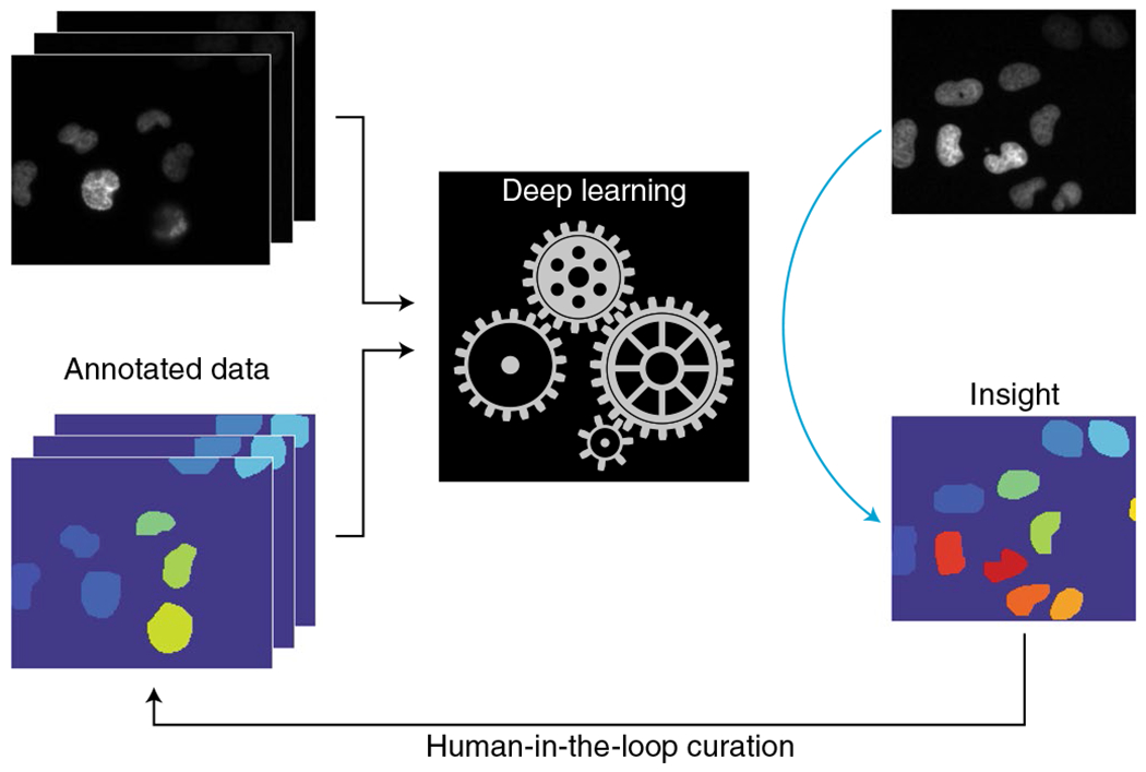
Annotations produced by expert annotators or by a crowd can be used to train deep learning models to extract insights from data. Once trained, these models can be deployed to process new, unannotated data. The human-in-the-loop extension involves the identification of model errors, error correction to produce new training data, and retraining on an updated dataset.
By focusing on use cases that are common in quantitative cell biology, this Review serves as a practical introduction to deep learning for the analysis of biological images. It builds on prior reviews of the intersection of deep learning and the life sciences42,45–47 by incorporating a discussion of our labs’ joint experiences in applying these methods to cellular imaging data, and is meant to make these methods less opaque to new adopters. First, we review the practical mechanics of deep learning, including the mathematical underpinnings, recent advances in neural-network architectures, and existing software frameworks. Next, we outline what we feel are the key components of effective, laboratory-scale deep learning solutions. We then review four use cases: image classification, image segmentation, object tracking, and augmented microscopy. For each use case, we cover problem specification, the state of the field with respect to algorithms and biological applications, and publicly available datasets. We close by sharing some of the lessons that our labs have learned while adapting these methods to biological data, and by suggesting directions for future work.
The practical mechanics of deep learning
In deep learning, an algorithm learns effective representations for a given task entirely from data. An introduction to the mathematics underlying the training of deep learning models is given in Box 1, troubleshooting advice is given in Box 2, and a glossary of commonly used terms is given in Box 3. Because the most successful solutions have been supervised, we believe that there are three essential components to the successful application of deep learning to biological image analysis: construction of a pertinent and annotated training dataset, effective training of deep learning models on that dataset, and deployment of trained models on new data.
Box 1 |. Training a linear image classifier.
To illustrate the workflow for training a deep learning model in a supervised manner, here we consider the case of training a linear classifier to recognize grayscale images of cats and dogs. Each image is an array of size (Nx, Ny, 1), where Nx and Ny are the number of pixels in the x and y dimensions, respectively, and 1 is the number of channels in the image. For this exercise, we collapse the image into a vector of size (NxNy, 1). The classification task is to construct a function that takes this vector as input and predicts a label (0 for cats, 1 for dogs). A linear classifier performs this task by producing class scores that are a linear function of each pixel value. Mathematically, this is written as
where y0 and y1 are the class scores, W is a matrix of class weights, and x is the image vector. The class with the highest score is the predicted class. The learning task then tunes the wi,j values so that a loss function that measures the classifier’s performance on some training dataset is minimized. A common loss function is the cross-entropy, or softmax, loss. To arrive at this loss function, we first transform our class scores y0 and y1 into probabilities by defining
These probabilities reflect the model’s certainty that an image belongs in class i. The loss evaluated for a collection of images is defined as
where pCorrect is the probability assigned to the correct class for that image. This equation has two terms. The first can be thought of as the negative log likelihood of choosing the correct class. The second term is called L2 regularization; it penalizes large weights to control against overfitting.
To minimize the loss function, most optimization algorithms used in deep learning are a variation of stochastic gradient descent. First, the weights are randomly initialized to some small value. The choice of initialization can affect the training of deep models considerably; best practices for initialization include the initialization settings of He et al.167. Next, we select a small batch of images, called a minibatch, and identify the direction in which to change the weights so that the loss function will be reduced the most when evaluated on that minibatch. We then perturb the weights a small amount in that direction. The correct direction in which to perturb the weights is captured by the gradient of the loss function with respect to the weights. Mathematically, this gradient leads to the update rule
where lr, the scalar that scales the gradient at each step, is the learning rate. For the case of the linear classifier, we can compute these gradients analytically. The gradient for one image is given by
where 1() is an indicator function that is 1 when the statement inside the parentheses is true and 0 when false. The gradient for the minibatch of images is the sum of the gradients for all images in the batch. This equation provides some information on how gradient descent changes the weights. The first term leads to an increase in weights that correspond to the correct class and a decrease in weights that correspond to the incorrect class. If the model is certain (pi ≈ 1) and correct, the contribution will be minimal; the opposite is true if the model is certain and wrong. The gradient is scaled by the relevant pixel value xj, which causes the model to pay attention to bright pixels. The contribution of the regularization term pushes weights toward zero, preventing any one weight from getting too big. Once the weights are updated, the user then selects another batch of images and repeats the process until the loss is sufficiently minimized. The accuracy and loss of the algorithm on the validation dataset are often used to develop stopping criteria. Training is often stopped when the validation loss ceases to improve or when the training and validation error curves start to diverge, signifying overfitting.
While the linear classifier highlights several key features of training, in practice there are some important differences. Variants of the loss function shown above have been developed to address issues surrounding class imbalance in datasets. Several variants of stochastic gradient descent exist, including with momentum168–170, RMSprop171, Adagrad172, Adadelta173, and Adam174. Recent work suggests that networks trained with stochastic gradient descent with momentum have better performance with respect to generalization175,176. We have presented the learning rate as a static parameter, but in practice it often decreases as training progresses.
Importantly, the mathematical structure of deep learning models is more complicated than the linear model presented here. While this simplification may appear problematic with respect to analytical computation of the gradients for training, all deep learning models are compositional. This allows one to iteratively use the chain rule177 to derive analytical expressions for the gradients, even for complicated functions, as shown in the figure in this box.
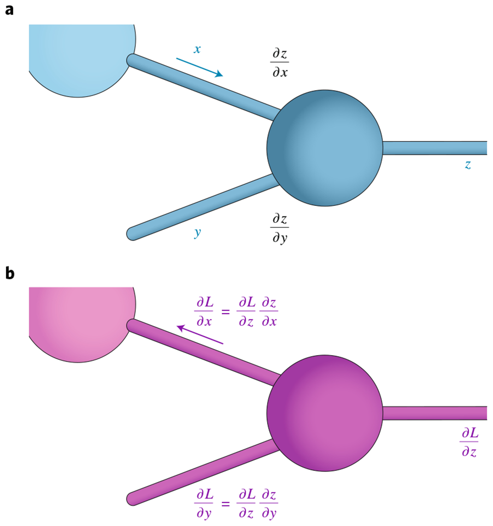
Computing gradients with backpropagation. a, During the forward pass, local derivatives are computed alongside the original computation. b, During the backward pass, the chain rule is used in conjunction with the local derivatives to compute the derivative of the loss function with respect to each weight.
Box 2 |. Troubleshooting.
While deep learning can solve many problems in biological image analysis, the creation of well-performing models often requires a substantial amount of troubleshooting. Here we provide guidance on navigating common issues that arise in the training of deep learning models.
Training performance.
Very poor performance during training, defined as a classification error equal to or worse than random chance, can usually be traced to an issue with data or with training parameters. For small datasets, errors in training data can lead to poor performance. These errors often go unnoticed until the training data are manually inspected. Improper image normalization can lead to poor performance, as images can lose their informative features. Errors in the code that performs image augmentation and feeds data into the training pipeline can also yield poor performance. The learning rate is often the first parameter to be adjusted when the training data are free of errors and the performance is still very poor. Changing the model architecture to increase model capacity can also be an effective solution.
Overfitting.
Deep learning models can learn complex relationships among data and annotations. As a result, there may be concern as to whether a deep learning model has learned something general that will work on real data or whether the model’s learning is unique to the training dataset. This phenomenon is called overfitting and is generally measured as the difference between model accuracy for a training dataset and that for a validation dataset. The amount of overfitting that can be tolerated varies by task; several percentage points may be tolerable for segmentation but might cause an image classifier to misclassify important rare categories. Several regularization techniques exist to mitigate overfitting, but they often come at the expense of model capacity. Batch normalization159 has strong regularization properties, as does dropout161. Typically, only one of these methods is used in a model, as performance can suffer if both are used simultaneously162. Increasing the strength of L2 regularization also mitigates overfitting, but at the expense of model capacity. Increasing the range of data-augmentation operations creates a more varied training dataset and hence more robust models49. Because overfitting often gets worse the longer that training proceeds, stopping training early can also be effective178. The choice of model architecture is especially important for small datasets. Architectures with large model capacities can be especially prone to overfitting on small datasets, although this tendency can be somewhat mitigated with transfer learning by pretraining on larger datasets50. Finally, the training algorithm used affects overfitting: recent work has demonstrated that models trained with stochastic gradient descent with momentum generalize better than models trained with other algorithms175,176.
Class imbalance.
Training datasets for classification tasks often have different numbers of examples for each label, which can lead to poorly performing models. As an example, consider a dataset in which 90% of the examples are label A and 10% are label B. The deep learning model may learn to predict everything as being class A and then report an overall classification accuracy of 90%. However, the reported accuracy is misleading, and the model is too inaccurate on class B to be used. There are several solutions to class imbalance. Resampling the training data to yield an identical number of elements in each class is one approach. This strategy can include downsampling to match the smallest class size, upsampling to match the largest class size, or both. Caution must be taken with downsampling when the least-represented class is much smaller (approximately tenfold) than all the other classes, as the diversity of the training data will be severely reduced. Another way to account for class imbalance is to introduce a class weight term into the loss function. This term, which is often taken as (NTotal examples/NExamples in class i) × (1/NClasses) for each class i, multiplies each example data’s individual contribution to the loss. This class weight term can be comPuted for the entire training dataset or for each minibatch on the fly.
Assessing performance.
Following performance metrics during and after training is an important part of creating deep learning models. For performance assessment, the training data are often split into two portions, one for training and one for validation. If the performance on the validation dataset is used to modify training parameters, then it is possible to overfit the model to the validation data, even though these data were not used explicitly during training. Therefore, some researchers split their data into three parts: one for training, one for validation during training, and one for testing real-world performance. Our groups have achieved good success by reserving 10–20% of annotated data for testing.
Once the dataset is split, the remaining issue is choosing a performance metric. As seen from the class imbalance example, simple metrics such as accuracy can misrepresent performance. Useful metrics vary by problem type. For classification tasks, assessment of the accuracy for each individual class is more informative than an average across all classes. A confusion matrix179 goes one step further, as it reveals the frequency of each type of misclassification. For segmentation tasks, both pixel-level (for example, the Dice and Jaccard indices180) and instance-level metrics (precision181, recall181, and mean average precision182) can be used to measure performance. Quantification of the rates at which specific errors occur, such as false splitting or merging of instance masks, has yielded important insights into the failure modes of deep learning models52. The appropriate metrics should be used on both training and validation datasets at the end of each training epoch.
Hyperparameter optimization.
A hyperparameter is a parameter that is set before learning begins. Hyperparameters include L2 regularization strength, learning rate, initialization settings for parameters, and details of the deep learning architecture (number of layers, types of layers, number of filters in each layer, etc.). The optimization of hyperparameters, an essential part of the training process for deep learning models, usually consists of three phases: selection of an initial condition, selection of an optimization objective, and a search to find the best hyperparameters. While choosing initial conditions can be tricky, packages like Keras come with best-practice default settings for hyperparameters such as learning rate, L2 regularization strength, and weight initialization59. In practice, our groups often use the per-class training and validation accuracies as targets, with the goal of maximizing the training accuracies across classes while minimizing the gap between training and validation accuracies to minimize overfitting. Finally, there are several strategies for searching hyperparameter space. Grid searches in which the learning rate and regularization strength are tuned are often effective. Model architecture can also be modified; our groups often use the tradeoff between model capacity and overfitting as a guide to determine the changes that should be made. Our prior work has shown that it is important to match a model’s receptive field size with the relevant feature size in order to produce a well-performing model for biological images48. The Python package Talos is a convenient tool for Keras59 users that helps to automate hyperparameter optimization through grid searches183.
Software engineering.
We have found that modern software-development practices have substantially improved the programming experience, as well as the stability of the underlying hardware. Our groups routinely use Git and Docker74 to develop and deploy deep learning models. Git is a version-control software, and the associated web platform GitHub allows code to be jointly developed by team members. Docker is a containerization tool that enables the production of reproducible programming environments.
Dimension mismatch.
Mismatches between the dimensions of adjacent layers are common errors that often arise. Although most frameworks automatically infer the dimension sizes for each layer, this error can still occur. Our typical solution is to map out the dimensions of each layer to identify and correct dimension mismatches.
Box 3 |. Glossary.
Deep learning: a set of machine-learning methods—specifically, neural networks—that are capable of learning representations from data with increasing levels of abstraction30.
Hyperparameter: a parameter whose value is set before training. Examples include the learning rate, L2 regularization strength, and deep learning model architecture.
Cross-validation: the use of held-out data to test model performance during training71. N-fold cross-validation splits data into N partitions and uses one of the partitions as validation data during an iteration through the training data.
Generalization: the ability of a machine-learning model to perform well on held-out data. Models that generalize have presumably learned important, general features of the data.
Underfitting: the inability of a machine-learning model to capture the variance present in training data71. Underfit models have suboptimal performance on training data.
Overfitting: the inability of a machine-learning model to perform well on held-out data, despite good performance on training data71. Overfit models learn features that are specific to the training data, which leads to reduced performance on held-out data. Overfitting can be quantified by measurement of the difference between a model’s classification error for training and testing data.
Model capacity: the representational power of a machine-learning model.
Transfer learning: repurposing of a trained machine-learning model for a new task. In deep learning, transfer learning entails training a model on a large dataset and then fine-tuning the model for a different task using a new, smaller dataset.
Epoch: one iteration through the entire training dataset during stochastic gradient descent.
Recall: the fraction of positive examples detected by a model181. Mathematically, for a two-class classification problem, recall is calculated as (True positives)/(True positives + False negatives).
Precision: the percentage of positive predictions from a model that are true181. Mathematically, for a two-class prediction problem, precision is calculated as (True positives)/(True positives + False positives).
Mean average precision: summary of the precision-recall score. For object detection, the mean average precision is defined as the mean of the precisions found at a set of equally spaced recall levels. Traditionally, 11 recall levels (0, 0.1, …, 1.0) are used182.
F1 score: the harmonic mean between precision and recall181. Mathematically, the F1 score is defined as 2((Precision × Recall)/(Precision + Recall)).
Jaccard index: a metric for segmentation accuracy180; intersection over union. Mathematically, if R is a reference segmentation and S is a predicted segmentation, then the Jaccard index is given by R ∩ S/R ∪ S.
Dice index: a metric for segmentation accuracy180, defined mathematically as 2 |R ∩ S|/(|R| + |S|).
Training data are critical to successful applications of deep learning; this requirement is one of the key disadvantages of this method. In our experience, assembling sufficient high-quality data often takes as much, if not more, time as programming the deep learning solution. Robust solutions require datasets that capture the diversity of images likely to be encountered during analysis. As much as possible, annotations for these datasets need to be error free, because errors can be learned. While training data may be limited, computational approaches can extract the most utility out of existing data. Image normalization reduces variation from distinct acquisition conditions42,48. Data-augmentation operations such as rotation, flipping, and zooming can also increase the image diversity in a limited dataset; these operations are generally standard practices regardless of the dataset size or type49. Transfer learning is another approach for creating robust models with limited data. In transfer learning, a deep learning model is trained on a large dataset to learn general image features, and then is fine-tuned on a smaller dataset to learn to perform a specific task50,51. While these approaches enable well-performing networks to emerge from limited datasets, considerable performance boosts arise from large annotated datasets52. For some uses, such as the detection of diffraction-limited spots, it has been possible to produce simulated images with a known annotation53. In other strategies, the curated outputs of traditional computer-vision pipelines have been used as training data54. Training data have also been produced manually by experts using annotation tools such as Fiji/ImageJ48, Cellprofiler52, and the Allen Cell Structure Segmenter55. Crowdsourcing, a cost-effective source of large datasets, is extensively used in fields such as automated driving; existing tools are being adapted for biological images. Enterprise commercial solutions include Figure Eight, which was recently acquired by Appen, and Samasource. The Quanti.us56 tool features a graphical user interface for biological image annotation for use on Amazon Mechanical Turk, as does Amazon’s Ground Truth tool, which uses active learning to reduce data-labeling costs. Gamification has also yielded some very promising results57. Importantly, the community acknowledges that the annotated datasets that power deep learning algorithms should be publicly available, as a comprehensive and expansive set of training data specific to biological problems would aid the development of deep learning algorithms considerably.
Once training data have been acquired, a deep learning model can be trained to accurately make predictions for new data. This task has several unique software and hardware requirements. Currently, Python is the most popular language for deep learning; existing frameworks include Tensorflow/Keras58,59, PyTorch60, MXNet61, CNTK62, Theano63, and Caffe64. Although these frameworks have important differences, there are also several commonalities. First, all of them construct a computation graph that outlines all the computations made by a deep learning model as input data are transformed into the final output. Second, they all automatically perform derivatives, which enables them to carry out optimizations like those described in Box 1 without additional work by the user once the computation graph is specified. Third, they provide an easy gateway for specialized hardware such as graphical processing units (GPUs) and tensor processing units65–67. Because deep learning models often contain millions of parameters, specialized hardware is needed to perform these computations quickly. Fourth, these frameworks all contain implementations of common mathematical objects, optimization algorithms, hyperparameter settings, and performance metrics—meaning that users can quickly apply deep learning to their data without having to reproduce these implementations on their own. Although a considerable amount of programming is still required to adapt these frameworks to cellular imaging data, they substantially reduce the barrier to entry.
These frameworks have greatly simplified the training and deployment of deep learning models. Programming aspects are often reduced to finding a deep learning architecture that yields the best performance for a particular task. Recent strategies have incorporated a search throughout the space of potential architectures to identify the most effective model architecture68–70 (Fig. 2). In our experience, the choice of architectural features often comes down to a tradeoff between overfitting and underfitting; this is also known as the bias–variance tradeoff in statistical modeling71 (Fig. 2j). Overfitting occurs when models perform well on a training dataset but perform poorly on a withheld validation dataset, whereas underfitting occurs when models perform poorly on training data because they are unable to capture the variation in a training dataset. These two outcomes are often (but not always) two faces of the same coin, which we call model capacity: the representational power of a deep learning model. Models with high model capacity perform well on large datasets but are prone to overfitting. Models with lower model capacity may generalize better but are at risk for underfitting. Overfit models can be unreliable on unseen data, and underfit models have suboptimal performance71. Overfitting is a particularly important issue with small datasets. Techniques for mitigating overfitting are discussed in Box 2 and Fig. 2j–m. Recent years have seen architectural advances, such as residual networks68, that have increased model capacity, which can lead to overfitting72. We recommend using model architectures with high model capacity only when enough data are present to avoid the model fragility that comes with overfitting. When data are limited, models with limited capacity and trained with regularization techniques are more likely to be robust. An alternative approach is to use transfer learning when adapting deep learning models to small datasets. This strategy often requires that pretrained models be modified to be compatible with the new dataset and task (changing the number of channels for an input image, etc.); users often are unable to make substantial changes to the model architecture. Despite these limitations, transfer learning can be very effective when data are limited. Whether training datasets are sufficiently large can be assessed with a cross-validation analysis. In this approach, one computes the degree of overfitting on models trained on varying fractions of the available training data. If the amount of data is sufficient, then the degree of overfitting should be stable even when the size of the training dataset is reduced. While overfitting is an important issue, other practical concerns come into play (Box 2), including optimization of hyperparameters such as the learning rate, choice of training algorithm, and issues surrounding class balancing.
Fig. 2 |. Common mathematical components of deep learning models.
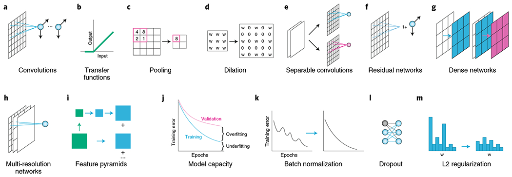
a, Convolutions extract local features in images, and the weights of each filter can be tuned to extract the best feature for a given dataset and task. b, Transfer functions such as those applied by the common rectified linear unit (ReLU) make possible the learning of nonlinear relationships. c, Pooling operations like max pooling downsample to produce spatially coarse feature maps154. Deep learning architectures often use iterative rounds of the three operations in a-c to produce low-dimensional representations of images. d, Dilations allow convolutional and pooling kernels to increase their spatial extent while keeping the number of parameters fixed48,155. When used correctly, dilations allow classification networks trained on image patches to be used for dense pixel-level prediction. e-i, Modern deep learning models make use of several architectural elements. e, Separable convolutions perform the convolution operation on each channel separately, which reduces the computing power while preserving accuracy156,157. f, Residual networks learn the identity mapping plus a small residual and enable the construction of very deep networks68. g, Dense networks allow each layer to see every prior layer69, which improves error propagation and encourages both feature reuse and parameter efficiency69,70. h, Multi-resolution networks allow the classification layers to see both fine and coarse feature maps86. i, Through feature pyramids, object-detection models detect objects at distinct length scales91,158. j, A plot of the training error during training reveals the relationships among overfitting, underfitting, and model capacity. The tradeoff among these attributes determines which network architectures are suitable for a given task. “Underfitting” refers to models with insufficient representational power, and “overfitting” refers to models that have learned features specific to training data and hence generalize poorly to new, unseen data. Increased model capacity reduces underfitting but can increase the risk of overfitting. k-m, Numerous regularization techniques ensure that deep learning models learn general features from data. k, Batch normalization both regularizes networks and reduces the time needed for training159. It was initially created to mitigate covariate shift but was recently found to smooth the landscape of the loss function160. l, Dropout randomly turns off filters during training161, which regularizes the network by forcing it to not overly rely on any one feature to make predictions. Batch normalization and dropout are typically not used together in the same model162. m, L2 regularization penalizes large weights and reduces overfitting.
Once trained, deep learning models must be deployed to process new data. While deployment can be achieved with scripts and Jupyter Notebooks48, an alternative and arguably more effective approach is to use built-in deployment tools in several frameworks. For instance, both Tensorflow and MXNet have built-in deployment features that enable models to be deployed on a server and accessed through standard internet communication protocols73, which allows the models to be shared beyond the original user. Associated software and hardware requirements mean that additional layers of software engineering beyond what is typical for academic software are often required for a deployment solution to be useful. First, containerization tools such as Docker74 have been essential for the creation of reproducible environments for developing and deploying deep learning models. Second, the need for GPUs has been a barrier, as a considerable amount of Unix system administration experience is necessary to ensure that all the requisite drivers and software packages are operational. While some vendors such as NVIDIA and Lambda Labs provide combined software and hardware solutions, increasingly, cloud computing is used because it both removes variability in hardware and enables users to match their computational power to their workload. Further, it empowers new users of deep learning by providing the requisite hardware quickly and affordably. The cloud was a key feature of the CDeep3M tool75 and was also used by Keren et al.11 to deploy deep learning models to quantify spatial proteomics data of the tumor microenvironment.
Biological applications of deep learning
Now, we discuss the application of deep learning to four critical use cases: image classification, image segmentation, object tracking, and augmented microscopy. For each use case, we describe the existing deep learning methodologies and their specific application to cellular analysis.
Image classification.
Image classification, the task of assigning a meaningful label to an image, was one of the first high-profile successes of deep learning. A classic example is the discrimination between images of cats and dogs; a biologically motivated example would be identifying whether a protein is expressed in the cytoplasm or the nucleus on the basis of fluorescence. A schematic of image classification and its biological application is shown in Fig. 3. Because of the utility of image classification, much of the recent work in computer vision has focused on improving performance on standard datasets such as ImageNet68,69. The architectures underlying biological applications are very similar to, if not the same as, those in commercial applications. Because of this similarity, and because of the relative lack of annotated training data for biological images, transfer learning has featured prominently in the creation of image classifiers that perform well on biological data50,76. One can implement transfer learning in these cases by starting with an image classifier that has been trained on a large dataset, such as ImageNet, replacing the final layer with one suitable for the new classification task, and then retraining on a smaller set of annotated data50.
Fig. 3 |. Image classification applied to biological images.
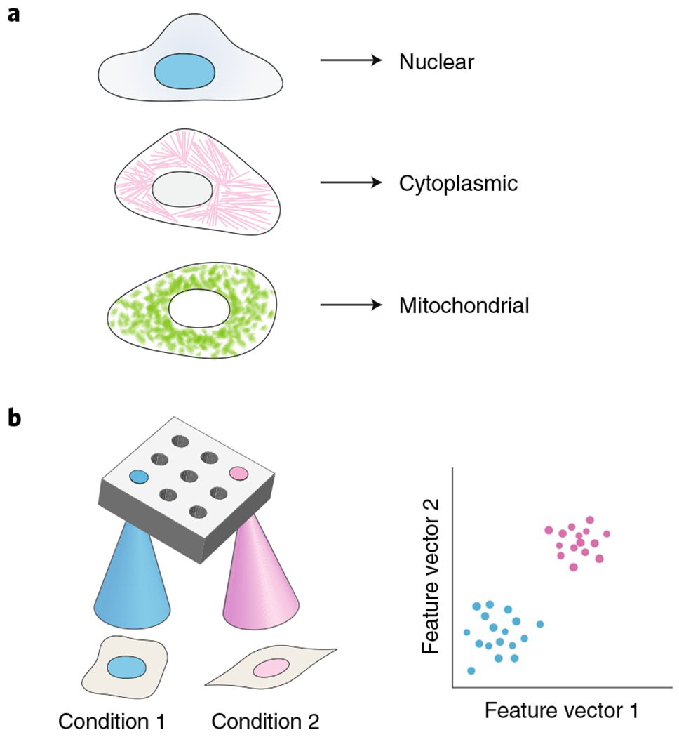
a, A deep-learning-based image classifier accurately identifies spatial patterns of protein expression in fluorescence images. b, Deep-learning-based image classifiers can accurately interpret changes in cell morphology in imaging-based high-throughput screening. These models are trained on classification tasks and then used to extract feature vectors from images, which can be clustered to identify novel cell phenotypes.
Previous applications of deep-learning-based image classification to biological data demonstrate the technical advantages of deep learning for biological discovery. For example, most work on the interpretation of imaging-based high-throughput screens has focused on the generation of classifiers that identify conditions and compounds that lead to meaningful changes in cell morphology77. To account for changes in cell morphology that might not be captured in labeled data, several approaches have used deep learning models to extract feature vectors instead of labels, and then clustered those vectors76,78,79. Image classifiers have also been used to identify changes in cell state79,80: in a recent study, scientists used a fluorescent marker of differentiation to establish a ground truth and then trained a classifier to identify differentiated cells directly from bright-field images81. Deep learning has also been used to classify spatial patterns in fluorescence images and to determine protein localization in large datasets from yeast82–84 and humans57. Last, deep-learning-based image classification was recently combined with microfluidics to produce a platform for intelligent, image-activated cell sorting85. Using this technology, Nitta et al.85 isolated cells on the basis of protein localization and cell-to-cell interactions. These studies highlight the fact that deep learning is an accessible tool that can help biologists understand their imaging data.
Image segmentation.
Image segmentation is the task of partitioning an image into several parts to identify meaningful objects or features (Fig. 4). One specific biological example is the need to identify single cells in microscope images, a common problem encountered in analyses of biological images. It is important to distinguish between semantic segmentation and instance segmentation because these two tasks feature prominently in the deep learning literature. Semantic segmentation is the task of partitioning an image into semantically meaningful parts and assigning each part a class label—for example, labeling each pixel of an image as cytoplasmic, nuclear, or background. Although this partitioning produces a pixel-level annotation, ‘object-ness’ is not necessarily preserved (in our example, two neighboring nuclei might not be separated into two distinct objects). In contrast, instance segmentation is the task of identifying each instance of a class in an image. Single-cell segmentation falls into this category and is the focus of this section. While there are numerous problems, such as spot detection in single-molecule experiments53, that have benefited from deep learning, and many more that eventually will, most of the available training data center on the identification of single cells through microscopy. All the approaches discussed below can be adapted to other image-segmentation problems through the collection of new, relevant training data.
Fig. 4 |. Image segmentation applied to biological images.
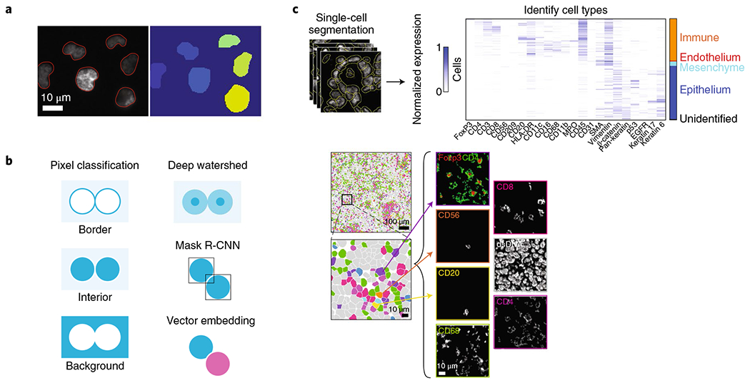
a, Instance segmentation identifies every instance of an object type, such as cell nuclei. b, Processing schema for instance segmentation. Pixel-classification approaches attempt to accurately predict object boundaries, deep watershed approaches learn a distance transform, object-detection methods predict a bounding box for each object, and embedding methods assign pixels in different objects to different vectors. c, Application of deep-learning-based image segmentation to spatial proteomics of breast cancer by Keren et al.11. Segmentation masks were used to measure signal intensity for each channel in each cell. This information was used by clustering algorithms to identify cell types and cell states. The ability to accurately segment single cells allowed Keren et al. to quantify immune behavior in the tumor microenvironment. Adapted with permission from ref. 11, Elsevier.
Deep learning schemas exist for instance segmentation; post-processing is particularly important (Fig. 4b). Two of the earliest software packages to apply deep-learning-enabled instance segmentation to single-cell analysis, U-Net43,86 and DeepCell48, treat segmentation as a pixel-level classification task and generate pixel-level predictions of cell interiors, cell edges, and background. Thresholding of the final probability maps yields the final segmentation mask. Deep learning has also been adapted to learn a distance transform (that is, how far a given pixel is from the image’s background), which can be fed into a watershed transform, a common computer-vision operation, to produce a final segmentation mask87. This approach was recently applied to single-cell segmentation, with very promising results88. Object-detection-based deep learning methods have also been adapted for instance segmentation. These methods, which include Faster R-CNN89 and Retinanet90, predict bounding boxes for all objects in an image and use non-maximum suppression to remove redundant bounding-box predictions. Mask R-CNN91, one of the most accurate methods for instance segmentation on general-purpose datasets, builds on these methods to predict an object mask for each bounding box. These methods have been successful when adapted to cellular data92–94. Recent work has treated the segmentation problem as a vector embedding problem95,96: a discriminative loss function assigns pixels in the same object to the same vector and pixels in different objects to different vectors, with unsupervised clustering on the embedding space identifying objects. This approach has yielded deep learning models that perform accurate instance segmentation even when objects overlap—a common case in images of cells. Last, generative approaches have recently been applied to segmentation, with promising results97–99.
While most of the models described here have focused on 2D segmentation, recent approaches have adapted these models to 3D data75,100. So far, there is no consensus approach to 2D or 3D data, and we suspect that the optimal method varies depending on the amount of training data and the segmentation task. For instance, bounding-box methods perform well on images of cell nuclei but might not be well suited to the segmentation of images of filamentous bacteria or fluorescent microtubules. We recommend that users focus their initial efforts on the existing DeepCell, CDeep3M, U-Net, CellProfiler, or Mask R-CNN software libraries, as these methods have been applied successfully to a variety of data types, provide pretrained models, and support both model training and deployment on new data.
The potential use cases of image segmentation are vast, and the improved accuracy of deep-learning-based approaches both automates traditional computer-vision workflows and makes previously impossible segmentation tasks possible. These approaches have been applied to the segmentation of neurons in images from cryo-electron microscopy101, with enough accuracy to place imaging-based connectomics within reach102. Single-cell image segmentation is another key application of this technology. U-Net86 was the first application of deep learning to single-cell analysis; work from our own groups has demonstrated that images of cells spanning the domains of life can be segmented with deep learning even with limited training data48. Larger datasets, such as those featured in the 2018 Kaggle Data Science Bowl103, render these approaches even more accurate52. Improved segmentation accuracy improves object tracking in both live-cell imaging and tracking of diffraction-limited objects. Accurate identification of the cytoplasm in mammalian cells improves the quantitation of localization-based live-cell reporters48,53 and was recently used to explore mechanisms of cell-size control in fission yeast104. Excitingly, deep learning recently was used for instance segmentation in pathology images99,105,106, positioning Keren et al.11 to quantify interactions between tumor cells and immune cells in spatial-proteomics measurements of formalin-fixed, paraffin-embedded tissues105 (Fig. 4c). We anticipate that deep learning will be critical for development of the Human Cell Atlas107,108, as image analysis is common to all spatial transcriptomics and proteomics experiments. Overall, easier deployment of machine-learning models should benefit nearly every experiment that involves cellular imaging. Links to existing tools for users who wish to apply these techniques to their own data are provided in Table 1.
Table 1 |.
Source code and containers for deep learning applications
| Application | Package name | Links and comments | Reference(s) |
|---|---|---|---|
| Image segmentation | DeepCell |
http://www.deepcell.org, http://github.com/vanvalenlab/deepcell-tf Software library for deep-learning-enabled single-cell analysis in the cloud. Users manage their own cloud deployment; model training and deployment are performed through a web interface. |
48,163 |
| Image segmentation | CDeep3M |
http://github.com/CRBS/cdeep3m Amazon machine image for training and deploying deep learning models for 2D and 3D image segmentation. |
75 |
| Image segmentation | U-Net |
http://github.com/lmb-freiburg/Unet-Segmentation ImageJ plug-in for single-cell image segmentation with U-Net. |
43,86 |
| Image segmentation | CellProfiler |
http://github.com/CellProfiler/CellProfiler Python-based software for single-cell segmentation and morphological profiling. Single-cell segmentation with U-Net available through a REST API. |
24,25 |
| Image segmentation | Mask R-CNN |
http://github.com/matterport/Mask_RCNN, https://github.com/fizyr/keras-retinanet, https://github.com/fizyr/keras-maskrcnn GitHub repositories with source code for implementations of Mask R-CNN and Retinanet. |
91 |
| Image classification | Cell Cognition Explorer |
https://software.cellcognition-project.org/ Source code for a Python-based tool for classifying cellular phenotypes with deep learning. |
79 |
| Object tracking and pose estimation | DeepLabCut |
http://alexemg.github.io/DeepLabCut/ Source code for object tracking and pose estimation with deep learning. |
128 |
| Object tracking and pose estimation | LEAP |
https://github.com/talmo/leap Source code for object tracking and pose estimation with deep learning. LEAP includes a GUI for data annotation. |
129 |
| Object tracking | idtracker.ai |
http://idtracker.ai/, https://gitlab.com/polavieja_lab/idtrackerai Source code for tracking animals with deep learning. idtracker.ai can track up to 100 animals in a single movie. |
130 |
| Augmented microscopy | In silico labeling |
http://www.allencell.org, http://github.com/google/in-silico-labeling Source code for predicting fluorescence images from bright-field images. |
139,142 |
| Augmented microscopy | Image restoration |
http://csbdeep.bioimagecomputing.com/ Source code for content aware image restoration (CARE). |
146 |
Object tracking.
Object tracking is the task of following objects through a series of time-lapse images. One example of a biological application of this is the tracking of single cells in live-cell imaging movies. During a typical movie, cells can move from one side of the imaging chamber to the other. Single-cell analysis requires that the cells be identified in every frame and that these detections be linked together over time. Although object tracking can be challenging, successful solutions have made it useful in a variety of biological analyses, including quantification of signaling dynamics109, efforts to understand cell motility110, and attempts to unravel the laws of bacterial cell growth111. The task is complex because of the number of objects in biological images—often hundreds to thousands—and complications that arise from image acquisition. Phototoxicity during imaging often limits the frame rate, and photobleaching causes objects to become dimmer over time. Objects can touch, disappear, merge (mitochondria or P-bodies), or split (e.g., by cell division). These issues have made it challenging to adapt existing object-tracking algorithms to biological data.
Object tracking consists of two tasks: object detection and object linkage. The optimal approach to object detection varies depending on the data. In many cases, objects can be represented as points; the object centroids in each frame are the information used for tracking. Classical approaches include nearest-neighbor search112, state-space models113–116, and linear programming117. When objects cannot be treated as points, instance segmentation is typically solved in each frame. In linear-programming approaches, multiple cues such as object centroids, intensity, and morphology are combined into a similarity score to link objects between frames118. Complex behaviors such as disappearance, splitting, and merging can be treated with linear programming, as in the now classic investigation by Jaqaman et al.119. In that work, a linear-assignment problem was solved to provide a globally optimal solution for both frame-by-frame object association and the assignment of division/splitting events to newly appeared or disappeared objects. This approach has been implemented in software packages such as uTrack119, CellProfiler24,25, and TrackMate120, which can be applied to images of particles or cells. Two recent investigations approached cell tracking in live-cell movies with probabilistic models121,122 and active contours123, with good success.
Deep learning has recently been adapted to track diffraction-limited particles, animals, and cells. While training data in this space are limited, software packages for curation are mitigating this issue121. Most work so far has focused on object detection, primarily because of limited training data; the 3D nature of object tracking means that training data are harder to produce. Nonetheless, deep learning improves segmentation accuracy, as tracking success is highly dependent on accurate identification of the objects to be tracked in every frame. For example, deep learning substantially improves object detection for particle tracking53, and work by us48 and others93,124 has shown that improved segmentation accuracy facilitates the tracking of cell nuclei in live-cell imaging. Deep learning has also been used to detect rare events such as mitosis; accurate detection of these events is likely to improve tracking performance125–127. The object-tracking package DeepLabCut, originally based on deep learning approaches to object detection and pose estimation, tracked appendages of flies and mice to quantify behavior during neuroscience experiments128. Impressively, by exploiting transfer learning, DeepLabCut performs remarkably well even with only a few dozen annotated examples. The recent software package LEAP129 builds on this work by incorporating a graphical user interface to assist in data annotation129, while the idtracker.ai130 software package tracks multiple organisms by using deep-learning-based image classifiers to identify animals that cross paths. Deep learning approaches to object linkage perform well on general-purpose datasets, by tracking a single object131–133, attempting to learn a similarity score directly from data for use in a linear-programming framework134, or treating tracking as a reinforcement learning problem135. Although promising, these approaches have yet to see extensive use with cellular images. One recent application used deep learning to segment and track single neurons in a time series of 3D images and to quantify calcium dynamics136. Interested users should first use deep learning to solve the object-detection portion of the tracking task. If this strategy does not sufficiently boost the performance of existing tracking algorithms, then relevant training data need to be collected and an appropriate deep-learning-based object linkage approach should be implemented.
Augmented microscopy.
Augmented microscopy is the extraction of latent information from biological images, such as the identification of the locations of cellular nuclei in bright-field images137. Although bright-field imaging methods such as phase-contrast microscopy and differential interference contrast microscopy can generate information on biological structures (e.g., the nucleus and the cytoplasm), it has been extremely difficult to computationally extract that information. Scientists solved this problem recently by recasting it as a supervised-learning problem (Fig. 5). Fluorescence images of biological structures serve as the ground truth, and the task is to predict this ground truth directly from the bright-field images138,139.
Fig. 5 |. Augmenting microscopy images with deep learning.
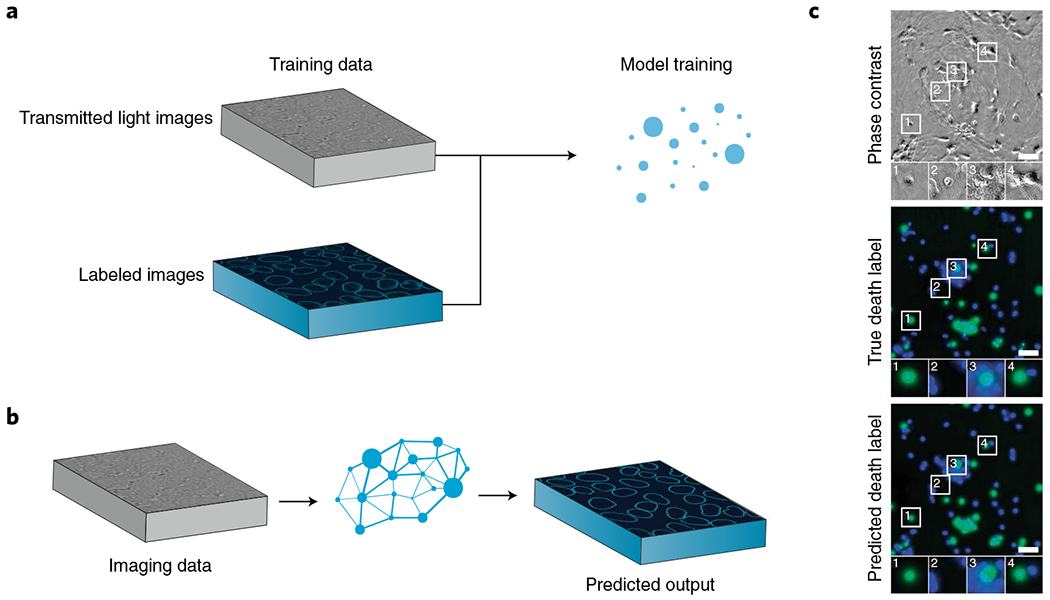
a, Deep learning accesses latent data in biological images by using fluorescence images of biological structures as a guide. This strategy yields predictions of fluorescence images and can also be used to improve image quality. b,c, This deep learning model infers which neurons are alive or dead directly from bright-field images. Adapted with permission from ref. 139, Elsevier.
Augmented microscopy is well suited to deep learning138–144. Each approach used so far has compared spatially synchronized transmitted light images with images from other modalities to uncover meaningful relationships among the corresponding images. For example, to create morphological models of the cell membrane and nucleus, researchers at the Allen Institute used a conditional generative model to create photo-realistic 3D fluorescence microscopy images, including the structural and functional information that the images are meant to represent, from 3D transmitted light microscopy images138,140,142,143. Their model featured two unique networks: one to learn variations in nucleus and cell shape, and another to learn the relationships among subcellular structures140. Researchers at Google, along with their external partners, used a modular approach to predict the location and intensity of various fluorescent labels on a per-pixel basis139. Their work made extensive use of multi-task and transfer learning to produce networks that were robust against varying imaging conditions, modalities, labels, sample types, and acquisition conditions. Their models were also trained on samples stained with propidium iodide, and thus their predictions included information on cell state and viability139.
Augmented microscopy is not limited to the association of fluorescence traces with transmitted light images145. Other groups use deep learning to provide content-aware image denoising146, to improve image resolution147, and to mitigate axial undersampling148 (to minimize phototoxicity) in real time. We anticipate that these new augmented-microscopy techniques will open the door to a new set of ‘computationally multiplexed’ experiments. While these computational approaches are currently restricted by the same limitations on training images (such as spectral limitations on probes), transfer learning on imaging platforms could enjoy a high degree of multiplexing10,12,149. These new tools are broadly applicable for improving image quality and overcoming limitations from spectral availability. Once the tools have been trained on broader datasets, bright-field images could be used as a source of supplementary ‘standard’ information (such as the locations of nuclei), freeing up spectral space for probes of other cell characteristics.
Looking forward
Although the application of deep learning to biological image analysis is still in its early days, there has already been remarkable progress in adapting deep learning to biological discovery. What can be done to encourage wider use of these tools? How can members of the field improve the performance of existing tools and support the development of new ones? First, there needs to be a concerted effort to produce large curated datasets that cover the image-analysis needs of most life scientists. This ‘cellular ImageNet’ should be open-access, as it will draw talented machine-learning scientists to biological problems. Attention must be paid to metadata, which will help researchers map their own acquisition conditions onto pre-existing datasets, thereby saving them the time currently needed to produce new annotations specific to their data. Given that crowdsourcing is likely to feature prominently in these efforts, we encourage sharing of crowdsourcing experiences—including common errors and solutions. We expect that tools for creating training data using a human-in-the-loop model150 will become increasingly valuable. Collections of models and model components pretrained on specific tasks would simplify the use of transfer learning; we expect tools like Tensorflow Hub to be valuable for this effort. Recent advances in neural architecture search151,152 may yield a set of deep learning architectures optimized for cellular image analysis. Importantly, good deployment solutions should be made accessible to new users while direct access to the code base is retained for advanced users. While the existing feature offerings for deep learning are impressive, we anticipate that they will be extended to new data types. For instance, cell segmentation should work in 2D and 3D tissues for multiple subcellular structures aside from the nucleus, such as the cytoplasm, plasma membrane, mitochondria, and endoplasmic reticulum. Augmented microscopy may be extended to predict 3D images from 2D data153 or to obtain high-quality confocal images from wide-field microscopy, and object tracking could be adapted to automate cell tracking and lineage construction. All these developments would greatly aid researchers who conduct live-cell imaging experiments and those involved in spatial genomics, by replacing existing analysis pipelines with more accurate deep learning counterparts, thus saving countless person-hours of curation. Additional applications are no doubt waiting to be uncovered. Finally, we recommend integrating tool building with biological discovery. Deep learning is a data science, and few know data better than those who acquire it. In our experience, better tools and better insights arise when bench scientists and computational scientists work side by side—even exchanging tasks—to drive discovery.
Acknowledgements
We thank A. Anandkumar, M. Angelo, L. Cai, S. Cooper, M. Elowitz, K.C. Huang, G. Johnson, A. Karpathy, L. Keren, A. Raj, T. Vora, and R. Wollman for helpful discussions and comments. This work was supported by several funding sources, including the Allen Discovery Center (award supporting W.G.; award supporting T.K., M.C., and D.V.V.), the Burroughs Wellcome Fund Postdoctoral Enrichment Program, a Figure Eight AI for Everyone award, and the NIH (subaward U24CA224309-01 to D.V.V.).
Footnotes
Competing interests
The authors declare no competing interests.
Data availability
Links to the data referred to in this Review can be found in Table 2.
Table 2 |.
Available datasets
| Application | Dataset | Links and comment | Reference(s) |
|---|---|---|---|
| Image classification | Human Protein Atlas |
http://www.proteinatlas.org Immunofluorescence images showing localization patterns of thousands of proteins for a variety of human cell lines. |
164 |
| Image classification and segmentation | Broad Bioimage Benchmark Collection |
http://data.broadinstitute.org/bbbc/ Single-cell annotations of fluorescent images of mammalian cells in cell culture. |
165 |
| Image segmentation | 2018 Kaggle Data Science Bowl |
http://www.kaggle.com/c/data-science-bowl-2018 Single-cell annotations of fluorescent images of mammalian cell nuclei in different contexts. |
103 |
| Image segmentation | DeepCell Dataset |
http://www.github.com/vanvalenlab/deepcell-tf, http://simtk.org/projects/deepcell Single-cell annotations of fluorescent images of mammalian cell nuclei and phase images of mammalian and bacterial cytoplasms. |
48,163 |
| Image segmentation | H&E-stained tissue slides from the Cancer Genome Atlas |
http://nucleisegmentationbenchmark.weebly.com/dataset.html Single-cell annotations of H&E-stained pathology images. |
106 |
| Object tracking | DeepLabCut |
http://www.mousemotorlab.org/deeplabcut/ Tracking and pose data for different organisms. |
128 |
| Object tracking | ISBI Cell Tracking Challenge |
http://www.celltrackingchallenge.net/ Segmentation and tracking data for mammalian cell nuclei and cytoplasm. |
166 |
| Augmented microscopy | Allen Institute for Cell Science |
http://www.allencell.org Augmented microscopy dataset. |
142 |
| Augmented microscopy | In silico labeling | http://github.com/google/in-silico-labeling/blob/master/data.md Augmented microscopy dataset. | 139 |
References
- 1.Grimm JB et al. A general method to fine-tune fluorophores for live-cell and in vivo imaging. Nat. Methods 14, 987–994 (2017). [DOI] [PMC free article] [PubMed] [Google Scholar]
- 2.Liu H et al. Visualizing long-term single-molecule dynamics in vivo by stochastic protein labeling. Proc. Natl. Acad. Sci. USA 115, 343–348 (2018). [DOI] [PMC free article] [PubMed] [Google Scholar]
- 3.Regot S, Hughey JJ, Bajar BT, Carrasco S & Covert MW High-sensitivity measurements of multiple kinase activities in live single cells. Cell 157, 1724–1734 (2014). [DOI] [PMC free article] [PubMed] [Google Scholar]
- 4.Sampattavanich S et al. Encoding growth factor identity in the temporal dynamics of FOXO3 under the combinatorial control of ERK and AKT kinases. Cell Syst. 6, 664–678 (2018). [DOI] [PMC free article] [PubMed] [Google Scholar]
- 5.Megason SG In toto imaging of embryogenesis with confocal time-lapse microscopy. Methods Mol. Biol. 546, 317–332 (2009). [DOI] [PMC free article] [PubMed] [Google Scholar]
- 6.Udan RS, Piazza VG, Hsu CW, Hadjantonakis A-K & Dickinson ME Quantitative imaging of cell dynamics in mouse embryos using light-sheet microscopy. Development 141, 4406–4414 (2014). [DOI] [PMC free article] [PubMed] [Google Scholar]
- 7.Chen B-C et al. Lattice light-sheet microscopy: imaging molecules to embryos at high spatiotemporal resolution. Science 346, 1257998 (2014). [DOI] [PMC free article] [PubMed] [Google Scholar]
- 8.Royer LA et al. Adaptive light-sheet microscopy for long-term, high-resolution imaging in living organisms. Nat. Biotechnol. 34, 1267–1278 (2016). [DOI] [PubMed] [Google Scholar]
- 9.McDole K et al. In toto imaging and reconstruction of post-implantation mouse development at the single-cell level. Cell 175, 859–876 (2018). [DOI] [PubMed] [Google Scholar]
- 10.Shah S, Lubeck E, Zhou W & Cai L seqFISH accurately detects transcripts in single cells and reveals robust spatial organization in the hippocampus. Neuron 94, 752–758 (2017). [DOI] [PubMed] [Google Scholar]
- 11.Keren L et al. A structured tumor-immune microenvironment in triple negative breast cancer revealed by multiplexed ion beam imaging. Cell 174, 1373–1387 (2018). [DOI] [PMC free article] [PubMed] [Google Scholar]
- 12.Lin J-R et al. Highly multiplexed immunofluorescence imaging of human tissues and tumors using t-CyCIF and conventional optical microscopes. eLife 7, e31657 (2018). [DOI] [PMC free article] [PubMed] [Google Scholar]
- 13.Caicedo JC et al. Data-analysis strategies for image-based cell profiling. Nat. Methods 14, 849–863 (2017). [DOI] [PMC free article] [PubMed] [Google Scholar]
- 14.van der Walt S, Colbert SC & Varoquaux G The NumPy array: a structure for efficient numerical computation. Comput. Sci. Eng 13, 22–30 (2011). [Google Scholar]
- 15.Jones E et al. SciPy: open source scientific tools for Python. https://www.scipy.org/ (2001).
- 16.McKinney W Data structures for statistical computing in Python. In Proc. 9th Python in Science Conference (eds. van der Walt S & Millman J) 51–56 (SciPy, 2010). [Google Scholar]
- 17.van der Walt S et al. scikit-image: image processing in Python. PeerJ 2, e453 (2014). [DOI] [PMC free article] [PubMed] [Google Scholar]
- 18.Pedregosa F et al. Scikit-learn: machine learning in Python. J. Mach. Learn. Res 12, 2825–2830 (2011). [Google Scholar]
- 19.Hunter JD Matplotlib: a 2D graphics environment. Comput. Sci. Eng 9, 90–95 (2007). [Google Scholar]
- 20.Kluyver T et al. Jupyter Notebooks—a publishing format for reproducible computational workflows. In Positioning and Power in Academic Publishing: Players, Agents and Agendas (eds. Loizides F & Schmidt B) 87–90 (IOS Press, 2016). [Google Scholar]
- 21.Stylianidou S, Brennan C, Nissen SB, Kuwada NJ & Wiggins PA SuperSegger: robust image segmentation, analysis and lineage tracking of bacterial cells. Mol. Microbiol 102, 690–700 (2016). [DOI] [PubMed] [Google Scholar]
- 22.Paintdakhi A et al. Oufti: an integrated software package for high-accuracy, high-throughput quantitative microscopy analysis. Mol. Microbiol 99, 767–777 (2016). [DOI] [PMC free article] [PubMed] [Google Scholar]
- 23.Ursell T et al. Rapid, precise quantification of bacterial cellular dimensions across a genomic-scale knockout library. BMC Biol. 15, 17 (2017). [DOI] [PMC free article] [PubMed] [Google Scholar]
- 24.Carpenter AE et al. CellProfiler: image analysis software for identifying and quantifying cell phenotypes. Genome Biol. 7, R100 (2006). [DOI] [PMC free article] [PubMed] [Google Scholar]
- 25.McQuin C et al. CellProfiler 3.0: next-generation image processing for biology. PLoS Biol. 16, e2005970 (2018). [DOI] [PMC free article] [PubMed] [Google Scholar]
- 26.Sommer C, Straehle C, Köthe U & Hamprecht FA Ilastik: interactive learning and segmentation toolkit. In 2011 IEEE International Symposium on Biomedical Imaging: From Nano to Macro (Wright S, Pan X & Liebling M) 230–233 (IEEE, 2011). [Google Scholar]
- 27.Belevich I, Joensuu M, Kumar D, Vihinen H & Jokitalo E Microscopy Image Browser: a platform for segmentation and analysis of multidimensional datasets. PLoS Biol. 14, e1002340 (2016). [DOI] [PMC free article] [PubMed] [Google Scholar]
- 28.Schindelin J et al. Fiji: an open-source platform for biological-image analysis. Nat. Methods 9, 676–682 (2012). [DOI] [PMC free article] [PubMed] [Google Scholar]
- 29.Allan C et al. OMERO: flexible, model-driven data management for experimental biology. Nat. Methods 9, 245–253 (2012). [DOI] [PMC free article] [PubMed] [Google Scholar]
- 30.LeCun Y, Bengio Y & Hinton G Deep learning. Nature 521, 436–444 (2015). [DOI] [PubMed] [Google Scholar]
- 31.Krizhevsky A, Sutskever I & Hinton GE ImageNet classification with deep convolutional neural networks. In Proc. 25th International Conference on Neural Information Processing Systems (eds. Pereira F et al. ) 1090–1098 (Curran Associates, 2012). [Google Scholar]
- 32.Carrasquilla J & Melko RG Machine learning phases of matter. Nat. Phys 13, 431–434 (2017). [DOI] [PMC free article] [PubMed] [Google Scholar]
- 33.Nguyen TQ et al. Topology classification with deep learning to improve real-time event selection at the LHC. Preprint available at https://arxiv.org/abs/1807.00083 (2018). [Google Scholar]
- 34.Castelvecchi D Artificial intelligence called in to tackle LHC data deluge. Nature 528, 18–19 (2015). [DOI] [PubMed] [Google Scholar]
- 35.Ramsundar B et al. Massively multitask networks for drug discovery. Preprint available at http://arxiv.org/abs/1502.02072 (2015). [Google Scholar]
- 36.Feinberg EN et al. Spatial graph convolutions for drug discovery. Preprint available at http://arxiv.org/abs/1803.04465 (2018). [Google Scholar]
- 37.Coudray N et al. Classification and mutation prediction from non-small cell lung cancer histopathology images using deep learning. Nat. Med 24, 1559–1567 (2018). [DOI] [PMC free article] [PubMed] [Google Scholar]
- 38.Esteva A et al. Dermatologist-level classification of skin cancer with deep neural networks. Nature 542, 115–118 (2017). [DOI] [PMC free article] [PubMed] [Google Scholar]
- 39.Poplin R et al. A universal SNP and small-indel variant caller using deep neural networks. Nat. Biotechnol. 36, 983–987 (2018). [DOI] [PubMed] [Google Scholar]
- 40.Zhou J et al. Deep learning sequence-based ab initio prediction of variant effects on expression and disease risk. Nat. Genet 50, 1171–1179 (2018). [DOI] [PMC free article] [PubMed] [Google Scholar]
- 41.Alipanahi B, Delong A, Weirauch MT & Frey BJ Predicting the sequence specificities of DNA-and RNA-binding proteins by deep learning. Nat. Biotechnol 33, 831–838 (2015). [DOI] [PubMed] [Google Scholar]
- 42.Angermueller C, Pärnamaa T, Parts L & Stegle O Deep learning for computational biology. Mol. Syst. Biol 12, 878 (2016). [DOI] [PMC free article] [PubMed] [Google Scholar]
- 43.Falk T et al. U-Net: deep learning for cell counting, detection, and morphometry. Nat. Methods 16, 67–70 (2019). [DOI] [PubMed] [Google Scholar]
- 44.Karpathy A Software 2.0. Medium https://medium.com/@karpathy/software-2-0-a64152b37c35 (2017). [Google Scholar]
- 45.Litjens G et al. A survey on deep learning in medical image analysis. Med. Image Anal 42, 60–88 (2017). [DOI] [PubMed] [Google Scholar]
- 46.Xing F, Xie F, Su H, Liu F & Yang L Deep learning in microscopy image analysis: a survey. IEEE Trans. Neural Netw. Learn. Syst 29, 4550–4568 (2018). [DOI] [PubMed] [Google Scholar]
- 47.Smith K et al. Phenotypic image analysis software tools for exploring and understanding big image data from cell-based assays. Cell Syst. 6, 636–653 (2018). [DOI] [PubMed] [Google Scholar]
- 48.Van Valen DA et al. Deep learning automates the quantitative analysis of individual cells in live-cell imaging experiments. PLOS Comput. Biol 12, e1005177 (2016). [DOI] [PMC free article] [PubMed] [Google Scholar]
- 49.Cire§an DC, Meier U, Gambardella LM & Schmidhuber J Deep, big, simple neural nets for handwritten digit recognition. Neural Comput. 22, 3207–3220 (2010). [DOI] [PubMed] [Google Scholar]
- 50.Zhang W et al. Deep model based transfer and multi-task learning for biological image analysis. IEEE Trans. Big Data 10.1109/TBDATA.2016.2573280 (2016). [DOI] [PMC free article] [PubMed] [Google Scholar]
- 51.Yosinski J, Clune J, Bengio Y & Lipson H How transferable are features in deep neural networks? In Proc. 27th International Conference on Neural Information Processing Systems (eds. Ghahramani Z et al. ) 3320–3328 (MIT Press, 2014). [Google Scholar]
- 52.Caicedo JC et al. Evaluation of deep learning strategies for nucleus segmentation in fluorescence images. Preprint available at https://www.biorxiv.org/content/early/2018/06/16/335216 (2018). [DOI] [PMC free article] [PubMed]
- 53.Newby JM, Schaefer AM, Lee PT, Forest MG & Lai SK Convolutional neural networks automate detection for tracking of submicron-scale particles in 2D and 3D. Proc. Natl. Acad. Sci. USA 115, 9026–9031 (2018). [DOI] [PMC free article] [PubMed] [Google Scholar]
- 54.Sadanandan SK, Ranefall P, Le Guyader S & Wählby C Automated training of deep convolutional neural networks for cell segmentation. Sci. Rep 7, 7860 (2017). [DOI] [PMC free article] [PubMed] [Google Scholar]
- 55.Chen J et al. The Allen Cell Structure Segmenter: a new open source toolkit for segmenting 3D intracellular structures in fluorescence microscopy images. Preprint available at https://www.biorxiv.org/content/early/2018/12/08/491035 (2018).
- 56.Hughes AJ et al. Quanti.us: a tool for rapid, flexible, crowd-based annotation of images. Nat. Methods 15, 587–590 (2018). [DOI] [PMC free article] [PubMed] [Google Scholar]
- 57.Sullivan DP et al. Deep learning is combined with massive-scale citizen science to improve large-scale image classification. Nat. Biotechnol 36, 820–828 (2018). [DOI] [PubMed] [Google Scholar]
- 58.Abadi M et al. TensorFlow: a system for large-scale machine learning. In Proc. 12th USENIX Conference on Operating Systems Design and Implementation (eds. Keeton K & Roscoe T) 265–283 (USENIX Association, 2016). [Google Scholar]
- 59.Chollet F Keras. GitHub https://github.com/keras-team/keras (2015). [Google Scholar]
- 60.Paszke A et al. Automatic differentiation in PyTorch. Oral presentation at NIPS 2017 Workshop on Automatic Differentiation, Long Beach, CA, USA, 9 December 2017. [Google Scholar]
- 61.Chen T et al. MXNet: a flexible and efficient machine learning library for heterogeneous distributed systems. Preprint available at http://arxiv.org/abs/1512.01274 (2015). [Google Scholar]
- 62.Seide F & Agarwal A CNTK: Microsoft’s open-source deep-learning toolkit. In Proc. 22nd ACM SIGKDD International Conference on Knowledge Discovery and Data Mining (eds. Krishnapuram B et al. ) 2135 (ACM, 2016). [Google Scholar]
- 63.Bergstra J et al. Theano: deep learning on GPUs with Python. Paper presented at Big Learning 2011: NIPS 2011 Workshop on Algorithms, Systems, and Tools for Learning at Scale, Sierra Nevada, Spain, 16–17 December 2011. [Google Scholar]
- 64.Jia Y et al. Caffe: convolutional architecture for fast feature embedding. In Proc. 22nd ACM International Conference on Multimedia (eds. Hua KA et al. ) 675–678 (ACM, 2014). [Google Scholar]
- 65.Jouppi NP et al. In-datacenter performance analysis of a tensor processing unit. In Proc. 44th Annual International Symposium on Computer Architecture (eds. Moshovos A et al. ) 1–12 (ACM, 2017). [Google Scholar]
- 66.Owens JD et al. GPU computing. Proc. IEEE 96, 879–899 (2008). [Google Scholar]
- 67.Chetlur S et al. cuDNN: efficient primitives for deep learning. Preprint available at http://arxiv.org/abs/1410.0759 (2014). [Google Scholar]
- 68.He K, Zhang X, Ren S & Sun J Deep residual learning for image recognition. In Proc. 29th IEEE Conference on Computer Vision and Pattern Recognition (eds. Agapito L et al. ) 770–778 (IEEE, 2016). [Google Scholar]
- 69.Huang G, Liu Z, van der Maaten L & Weinberger KQ Densely connected convolutional networks. In 2017 IEEE Conference on Computer Vision and Pattern Recognition (CVPR) (eds. Liu Y et al. ) 2261–2269 (IEEE, 2017). [Google Scholar]
- 70.Pelt DM & Sethian JA A mixed-scale dense convolutional neural network for image analysis. Proc. Natl. Acad. Sci. USA 115, 254–259 (2018). [DOI] [PMC free article] [PubMed] [Google Scholar]
- 71.Bishop CM Pattern Recognition and Machine Learning (Information Science and Statistics) (Springer-Verlag, 2006). [Google Scholar]
- 72.Ebrahimi MS & Abadi HK Study of residual networks for image recognition. Preprint available at http://arxiv.org/abs/1805.00325 (2018). [Google Scholar]
- 73.Richardson L & Ruby S RESTful Web Services (O’Reilly Media, 2007). [Google Scholar]
- 74.Merkel D Docker: lightweight Linux containers for consistent development and deployment. Linux J. 2014, 2 (2014). [Google Scholar]
- 75.Haberl MG et al. CDeep3M-Plug-and-Play cloud-based deep learning for image segmentation. Nat. Methods 15, 677–680 (2018). [DOI] [PMC free article] [PubMed] [Google Scholar]
- 76.Pawlowski N, Caicedo JC, Singh S, Carpenter AE & Storkey A Automating morphological profiling with generic deep convolutional networks. Preprint available at https://www.biorxiv.org/content/early/2016/11/02/085118 (2016).
- 77.Godinez WJ, Hossain I, Lazic SE, Davies JW & Zhang X A multi-scale convolutional neural network for phenotyping high-content cellular images. Bioinformatics 33, 2010–2019 (2017). [DOI] [PubMed] [Google Scholar]
- 78.Kandaswamy C, Silva LM, Alexandre LA & Santos JM High-content analysis of breast cancer using single-cell deep transfer learning. J. Biomol. Screen 21, 252–259 (2016). [DOI] [PubMed] [Google Scholar]
- 79.Sommer C, Hoefler R, Samwer M & Gerlich DW A deep learning and novelty detection framework for rapid phenotyping in high-content screening. Mol. Biol. Cell 28, 3428–3436 (2017). [DOI] [PMC free article] [PubMed] [Google Scholar]
- 80.Simm J et al. Repurposing high-throughput image assays enables biological activity prediction for drug discovery. Cell Chem. Biol 25, 611–618 (2018). [DOI] [PMC free article] [PubMed] [Google Scholar]
- 81.Buggenthin F et al. Prospective identification of hematopoietic lineage choice by deep learning. Nat. Methods 14, 403–406 (2017). [DOI] [PMC free article] [PubMed] [Google Scholar]
- 82.Kraus OZ, Ba JL & Frey BJ Classifying and segmenting microscopy images with deep multiple instance learning. Bioinformatics 32, i52–i59 (2016). [DOI] [PMC free article] [PubMed] [Google Scholar]
- 83.Kraus OZ et al. Automated analysis of high-content microscopy data with deep learning. Mol. Syst. Biol 13, 924 (2017). [DOI] [PMC free article] [PubMed] [Google Scholar]
- 84.Pärnamaa T & Parts L Accurate classification of protein subcellular localization from high-throughput microscopy images using deep learning. G3 (Bethesda) 7, 1385–1392 (2017). [DOI] [PMC free article] [PubMed] [Google Scholar]
- 85.Nitta N et al. Intelligent image-activated cell sorting. Cell 175, 266–276 (2018). [DOI] [PubMed] [Google Scholar]
- 86.Ronneberger O, Fischer P & Brox T U-Net: convolutional networks for biomedical image segmentation. In Medical Image Computing and Computer-Assisted Intervention—MICCAI 2015 (eds. Navab N et al. ) 234–241 (Springer, 2015). [Google Scholar]
- 87.Bai M & Urtasun R Deep watershed transform for instance segmentation. In 2017 IEEE Conference on Computer Vision and Pattern Recognition (CVPR) (eds. Liu Y et al. ) 2858–2866 (IEEE, 2017). [Google Scholar]
- 88.Wang W et al. Learn to segment single cells with deep distance estimator and deep cell detector. Preprint available at https://arxiv.org/abs/1803.10829 (2018). [DOI] [PMC free article] [PubMed] [Google Scholar]
- 89.Ren S, He K, Girshick R & Sun J Faster R-CNN: towards real-time object detection with region proposal networks. In Advances in Neural Information Processing Systems 28 (eds. Cortes C et al. ) 91–99 (Curran Associates, 2015). [Google Scholar]
- 90.Lin T, Goyal P, Girshick R, He K & Dollar P Focal loss for dense object detection. In 2017 IEEE International Conference on Computer Vision (ICCV) (eds. Ikeuchi K et al. ) 2999–3007 (IEEE, 2018). [Google Scholar]
- 91.He K, Gkioxari G, Dollar P & Girshick R Mask R-CNN. In 2017 IEEE International Conference on Computer Vision (ICCV) (eds. Ikeuchi K et al. ) 2980–2988 (IEEE, 2018). [Google Scholar]
- 92.Johnson JW Adapting Mask-RCNN for automatic nucleus segmentation. Preprint available at http://arxiv.org/abs/1805.00500 (2018). [Google Scholar]
- 93.Tsai H-F, Gajda J, Sloan TFW, Rares A & Shen AQ Usiigaci: instance-aware cell tracking in stain-free phase contrast microscopy enabled by machine learning. Preprint available at https://www.biorxiv.org/content/early/2019/01/18/524041 (2019).
- 94.Hollandi R et al. A deep learning framework for nucleus segmentation using image style transfer. Preprint available at https://www.biorxiv.org/content/10.1101/580605v1 (2019). [DOI] [PMC free article] [PubMed]
- 95.De Brabandere B, Neven D & Van Gool L Semantic instance segmentation with a discriminative loss function. In 2017 IEEE Conference on Computer Vision and Pattern Recognition Workshops (eds. Liu Y et al. ) 478–480 (IEEE, 2017). [Google Scholar]
- 96.Payer C, Štern D, Neff T, Bischof H & Urschler M Instance segmentation and tracking with cosine embeddings and recurrent hourglass networks. In Medical Image Computing and Computer Assisted Intervention—MICCAI 2018 (eds. Frangi AF et al. ) 3–11 (Springer, 2018). [Google Scholar]
- 97.Zhu J-Y, Park T, Isola P & Efros AA Unpaired image-to-image translation using cycle-consistent adversarial networks. Preprint available at http://arxiv.org/abs/1703.10593 (2017). [Google Scholar]
- 98.Haering M, Grosshans J, Wolf F & Eule S Automated segmentation of epithelial tissue using cycle-consistent generative adversarial networks. Preprint available at https://www.biorxiv.org/content/early/2018/04/30/311373 (2018).
- 99.Mahmood F et al. Deep adversarial training for multi-organ nuclei segmentation in histopathology images. Preprint available at http://arxiv.org/abs/1810.00236 (2018). [DOI] [PMC free article] [PubMed] [Google Scholar]
- 100.Tokuoka Y et al. Convolutional neural network-based instance segmentation algorithm to acquire quantitative criteria of early mouse development. Preprint available at https://www.biorxiv.org/content/early/2018/06/01/324186 (2018).
- 101.Januszewski M et al. High-precision automated reconstruction of neurons with flood-filling networks. Nat. Methods 15, 605–610 (2018). [DOI] [PubMed] [Google Scholar]
- 102.Li PH et al. Automated reconstruction of a serial-section EM Drosophila brain with flood-filling networks and local realignment. Preprint at https://www.biorxiv.org/content/10.1101/605634v1 (2019).
- 103.Booz Allen Hamilton. 2018 Data Science Bowl. Kaggle https://www.kaggle.com/c/data-science-bowl-2018 (2018).
- 104.Facchetti G, Knapp B, Flor-Parra I, Chang F & Howard M Reprogramming Cdr2-dependent geometry-based cell size control in fission yeast. Curr. Biol 29, 350–358 (2019). [DOI] [PMC free article] [PubMed] [Google Scholar]
- 105.Khoshdeli M, Winkelmaier G & Parvin B Fusion of encoder-decoder deep networks improves delineation of multiple nuclear phenotypes. BMC Bioinforma. 19, 294 (2018). [DOI] [PMC free article] [PubMed] [Google Scholar]
- 106.Kumar N et al. A dataset and a technique for generalized nuclear segmentation for computational pathology. IEEE Trans. Med. Imaging 36, 1550–1560 (2017). [DOI] [PubMed] [Google Scholar]
- 107.Regev A et al. The Human Cell Atlas. eLife 6, e27041 (2017). [DOI] [PMC free article] [PubMed] [Google Scholar]
- 108.Rozenblatt-Rosen O, Stubbington MJT, Regev A & Teichmann SA The Human Cell Atlas: from vision to reality. Nature 550, 451–453 (2017). [DOI] [PubMed] [Google Scholar]
- 109.Purvis JE & Lahav G Encoding and decoding cellular information through signaling dynamics. Cell 152, 945–956 (2013). [DOI] [PMC free article] [PubMed] [Google Scholar]
- 110.Kimmel JC, Chang AY, Brack AS & Marshall WF Inferring cell state by quantitative motility analysis reveals a dynamic state system and broken detailed balance. PLoS Comput. Biol. 14, e1005927 (2018). [DOI] [PMC free article] [PubMed] [Google Scholar]
- 111.Wang P et al. Robust growth of Escherichia coli. Curr. Biol 20, 1099–1103 (2010). [DOI] [PMC free article] [PubMed] [Google Scholar]
- 112.Dow JA, Lackie JM & Crocket KV A simple microcomputer-based system for real-time analysis of cell behaviour. J. Cell Sci 87, 171–182 (1987). [DOI] [PubMed] [Google Scholar]
- 113.Levine MD, Youssef YM, Noble PB & Boyarsky A The quantification of blood cell motion by a method of automatic digital picture processing. IEEE Trans. Pattern Anal. Mach. Intell PAMI-2, 444–450 (1980). [Google Scholar]
- 114.Smal I, Niessen W & Meijering E Bayesian tracking for fluorescence microscopic imaging. In 3rd IEEE International Symposium on Biomedical Imaging: Macro to Nano, 2006 (eds. Kovačević J et al. ) 550–553 (IEEE, 2006). [Google Scholar]
- 115.Godinez W et al. Tracking of virus particles in time-lapse fluorescence microscopy image sequences. In 2007 4th IEEE International Symposium on Biomedical Imaging: From Nano to Macro (eds. Fessler J et al. ) 256–259 (IEEE, 2007). [Google Scholar]
- 116.Ngoc SN, Briquet-Laugier F, Boulin C & Olivo J-C Adaptive detection for tracking moving biological objects in video microscopy sequences. In Proc. International Conference on Image Processing (eds. Chang S-F et al. ) 484–487 (IEEE, 1997). [Google Scholar]
- 117.Kachouie NN & Fieguth PW Extended-Hungarian-JPDA: exact single-frame stem cell tracking. IEEE Trans. Biomed. Eng 54, 2011–2019 (2007). [DOI] [PubMed] [Google Scholar]
- 118.Meijering E, Dzyubachyk O, Smal I & van Cappellen WA Tracking in cell and developmental biology. Semin. Cell Dev. Biol 20, 894–902 (2009). [DOI] [PubMed] [Google Scholar]
- 119.Jaqaman K et al. Robust single-particle tracking in live-cell time-lapse sequences. Nat. Methods 5, 695–702 (2008). [DOI] [PMC free article] [PubMed] [Google Scholar]
- 120.Tinevez J-Y et al. TrackMate: an open and extensible platform for single-particle tracking. Methods 115, 80–90 (2017). [DOI] [PubMed] [Google Scholar]
- 121.Cooper S, Barr AR, Glen R & Bakal C NucliTrack: an integrated nuclei tracking application. Bioinformatics 33, 3320–3322 (2017). [DOI] [PMC free article] [PubMed] [Google Scholar]
- 122.Magnusson KEG, Jalden J, Gilbert PM & Blau HM Global linking of cell tracks using the Viterbi algorithm. IEEE Trans. Med. Imaging 34, 911–929 (2015). [DOI] [PMC free article] [PubMed] [Google Scholar]
- 123.Amat F et al. Fast, accurate reconstruction of cell lineages from large-scale fluorescence microscopy data. Nat. Methods 11, 951–958 (2014). [DOI] [PubMed] [Google Scholar]
- 124.Akram SU, Kannala J, Eklund L & Heikkilä J Cell tracking via proposal generation and selection. Preprint available at https://arxiv.org/abs/1705.03386 (2017). [Google Scholar]
- 125.Cire§an DC, Giusti A, Gambardella LM & Schmidhuber J Mitosis detection in breast cancer histology images with deep neural networks. In Medical Image Computing and Computer-Assisted Intervention—MICCAI 2013 (eds. Mori K et al. ) 411–418 (Springer, 2013). [DOI] [PubMed] [Google Scholar]
- 126.Nie W-Z, Li W-H, Liu A-A, Hao T & Su Y-T 3D convolutional networks-based mitotic event detection in time-lapse phase contrast microscopy image sequences of stem cell populations. In 2016 IEEE Conference on Computer Vision and Pattern Recognition Workshops (eds. Agapito L et al. ) 55–62 (IEEE, 2016). [Google Scholar]
- 127.Mao Y & Yin Z A hierarchical convolutional neural network for mitosis detection in phase-contrast microscopy images. In Medical Image Computing and Computer-Assisted Intervention—MICCAI 2016 (eds. Ourselin S et al. ) 685–692 (Springer, 2016). [Google Scholar]
- 128.Mathis A et al. DeepLabCut: markerless pose estimation of user-defined body parts with deep learning. Nat. Neurosci 21, 1281–1289 (2018). [DOI] [PubMed] [Google Scholar]
- 129.Pereira TD et al. Fast animal pose estimation using deep neural networks. Nat. Methods 16, 117–125 (2019). [DOI] [PMC free article] [PubMed] [Google Scholar]
- 130.Romero-Ferrero F, Bergomi MG, Hinz RC, Heras FJH & de Polavieja GG idtracker.ai: tracking all individuals in small or large collectives of unmarked animals. Nat. Methods 16, 179–182 (2019). [DOI] [PubMed] [Google Scholar]
- 131.Gordon D, Farhadi A & Fox D Re3 : real-time recurrent regression networks for visual tracking of generic objects. IEEE Robot. Autom. Lett 3, 788–795 (2018). [Google Scholar]
- 132.Cui Z, Xiao S, Feng J & Yan S Recurrently target-attending tracking. In 2016 IEEE Conference on Computer Vision and Pattern Recognition (eds. Agapito L et al. ) 1449–1458 (IEEE, 2016). [Google Scholar]
- 133.Wang Y, Mao H & Yi Z Stem cell motion-tracking by using deep neural networks with multi-output. Neural Comput. Appl 10.1007/s00521-017-3291-2 (2017). [DOI] [Google Scholar]
- 134.Sadeghian A, Alahi A & Savarese S Tracking the untrackable: learning to track multiple cues with long-term dependencies. In 2017 IEEE International Conference on Computer Vision (eds. Ikeuchi K et al. ) 300–311 (IEEE, 2017). [Google Scholar]
- 135.Zhang D, Maei H, Wang X & Wang Y-F Deep reinforcement learning for visual object tracking in videos. Preprint available at http://arxiv.org/abs/1701.08936 (2017). [Google Scholar]
- 136.Wen C et al. Deep-learning-based flexible pipeline for segmenting and tracking cells in 3D image time series for whole brain imaging. Preprint available at https://www.biorxiv.org/content/early/2018/08/06/385567 (2018).
- 137.Sullivan DP & Lundberg E Seeing more: a future of augmented microscopy. Cell 173, 546–548 (2018). [DOI] [PubMed] [Google Scholar]
- 138.Ounkomol C et al. Three dimensional cross-modal image inference: label-free methods for subcellular structure prediction. Preprint available at https://www.biorxiv.org/content/10.1101/216606v4 (2017).
- 139.Christiansen EM et al. In silico labeling: predicting fluorescent labels in unlabeled images. Cell 173, 792–803 (2018). [DOI] [PMC free article] [PubMed] [Google Scholar]
- 140.Johnson GR, Donovan-Maiye RM & Maleckar MM Building a 3D integrated cell. Preprint available at https://www.biorxiv.org/content/early/2017/12/21/238378 (2017).
- 141.Osokin A, Chessel A, Salas REC & Vaggi F GANs for biological image synthesis. In 2017 IEEE International Conference on Computer Vision (eds. Ikeuchi K et al. ) 2252–2261 (IEEE, 2017). [Google Scholar]
- 142.Ounkomol C, Seshamani S, Maleckar MM, Collman F & Johnson GR Label-free prediction of three-dimensional fluorescence images from transmitted-light microscopy. Nat. Methods 15, 917–920 (2018). [DOI] [PMC free article] [PubMed] [Google Scholar]
- 143.Johnson G, Donovan-Maiye R, Ounkomol C & Maleckar MM Studying stem cell organization using “label-free” methods and a novel generative adversarial model. Biophys. J 114, 43a (2018). [Google Scholar]
- 144.Stumpe M & Mermel C An augmented reality microscope for cancer detection. Google AI Blog https://ai.googleblog.com/2018/04/an-augmented-reality-microscope.html (2018). [Google Scholar]
- 145.Belthangady C & Royer LA Applications, promises, and pitfalls of deep learning for fluorescence image reconstruction. Preprint available at https://www.preprints.org/manuscript/201812.0137/v1 (2018). [DOI] [PubMed]
- 146.Weigert M et al. Content-aware image restoration: pushing the limits of fluorescence microscopy. Preprint available at https://www.biorxiv.org/content/early/2018/07/03/236463 (2018). [DOI] [PubMed]
- 147.Wang H et al. Deep learning achieves super-resolution in fluorescence microscopy. Preprint available at https://www.biorxiv.org/content/early/2018/04/27/309641 (2018).
- 148.Rivenson Y et al. Deep learning microscopy. Optica 4, 1437–1443 (2017). [Google Scholar]
- 149.Angelo M et al. Multiplexed ion beam imaging of human breast tumors. Nat. Med 20, 436–442 (2014). [DOI] [PMC free article] [PubMed] [Google Scholar]
- 150.Acuna D, Ling H, Kar A & Fidler S Efficient interactive annotation of segmentation datasets with Polygon-RNN++. Preprint available at http://arxiv.org/abs/1803.09693 (2018). [Google Scholar]
- 151.Zoph B & Le QV Neural architecture search with reinforcement learning. Preprint available at http://arxiv.org/abs/1611.01578 (2016). [Google Scholar]
- 152.Zoph B, Vasudevan V, Shlens J & Le QV Learning transferable architectures for scalable image recognition. In Proc. 2018 IEEE/CVF Conference on Computer Vision and Pattern Recognition (eds. Forsyth D et al. ) 8697–8710 (IEEE, 2018). [Google Scholar]
- 153.Jackson AS, Bulat A, Argyriou V & Tzimiropoulos G Large pose 3D face reconstruction from a single image via direct volumetric CNN regression. Preprint available at http://arxiv.org/abs/1703.07834 (2017). [Google Scholar]
- 154.Nair V & Hinton GE Rectified linear units improve restricted Boltzmann machines. In Proc. 27th International Conference on Machine Learning (eds. Fürnkranz J & Joachims T) 807–814 (Omnipress, 2010). [Google Scholar]
- 155.Li H, Zhao R & Wang X Highly efficient forward and backward propagation of convolutional neural networks for pixelwise classification. Preprint available at http://arxiv.org/abs/1412.4526 (2014). [Google Scholar]
- 156.Chollet F Xception: deep learning with depthwise separable convolutions. In Proc. 30th IEEE Conference on Computer Vision and Pattern Recognition (eds. Liu Y et al. ) 1800–1807 (IEEE, 2017). [Google Scholar]
- 157.Howard AG et al. MobileNets: efficient convolutional neural networks for mobile vision applications. Preprint available at https://arxiv.org/abs/1704.04861v1 (2017). [Google Scholar]
- 158.Lin T et al. Feature pyramid networks for object detection. In Proc. 30th IEEE Conference on Computer Vision and Pattern Recognition (eds. Liu Y et al. ) 936–944 (IEEE, 2017). [Google Scholar]
- 159.Ioffe S & Szegedy C Batch normalization: accelerating deep network training by reducing internal covariate shift. Preprint available at http://arxiv.org/abs/1502.03167 (2015). [Google Scholar]
- 160.Santurkar S, Tsipras D, Ilyas A & Madry A How does batch normalization help optimization? (No, it is not about internal covariate shift). Preprint available at http://arxiv.org/abs/1805.11604 (2018). [Google Scholar]
- 161.Srivastava N, Hinton G, Krizhevsky A, Sutskever I & Salakhutdinov R Dropout: a simple way to prevent neural networks from overfitting. J. Mach. Learn. Res 15, 1929–1958 (2014). [Google Scholar]
- 162.Li X, Chen S, Hu X & Yang J Understanding the disharmony between dropout and batch normalization by variance shift. Preprint available at http://arxiv.org/abs/1801.05134 (2018). [Google Scholar]
- 163.Bannon D et al. DeepCell 2.0: automated cloud deployment of deep learning models for large-scale cellular image analysis. Preprint available at https://www.biorxiv.org/content/early/2018/12/22/505032 (2018).
- 164.Thul PJ et al. A subcellular map of the human proteome. Science 356, eaal3321 (2017). [DOI] [PubMed] [Google Scholar]
- 165.Ljosa V, Sokolnicki KL & Carpenter AE Annotated high-throughput microscopy image sets for validation. Nat. Methods 9, 637 (2012). [DOI] [PMC free article] [PubMed] [Google Scholar]
- 166.Maška M et al. A benchmark for comparison of cell tracking algorithms. Bioinformatics 30, 1609–1617 (2014). [DOI] [PMC free article] [PubMed] [Google Scholar]
- 167.He K, Zhang X, Ren S & Sun J Delving deep into rectifiers: surpassing human-level performance on ImageNet classification. In Proc. 2015 IEEE International Conference on Computer Vision (eds. Bajcsy R et al. ) 1026–1034 (IEEE, 2015). [Google Scholar]
- 168.Polyak BT Some methods of speeding up the convergence of iteration methods. USSR Comput. Math. Math. Phys 4, 1–17 (1964). [Google Scholar]
- 169.Nesterov YE A method for solving the convex programming problem with convergence rate O (1/k2). Dokl. Akad. Nauk SSSR 269, 543–547 (1983). [Google Scholar]
- 170.Sutskever I, Martens J, Dahl G & Hinton G On the importance of initialization and momentum in deep learning. Proc. Mach. Learn. Res 28, 1139–1147 (2013). [Google Scholar]
- 171.Tieleman T & Hinton G Neural Networks for Machine Learning lecture 6.5—rmsprop: divide the gradient by a running average of its recent magnitude. Coursera https://www.coursera.org/learn/neural-networks (2012).
- 172.Duchi J, Hazan E & Singer Y Adaptive subgradient methods for online learning and stochastic optimization. J. Mach. Learn. Res 12, 2121–2159 (2011). [Google Scholar]
- 173.Zeiler MD ADADELTA: an adaptive learning rate method. Preprint available at http://arxiv.org/abs/1212.5701 (2012). [Google Scholar]
- 174.Kingma DP & Ba J Adam: a method for stochastic optimization. Preprint available at http://arxiv.org/abs/1412.6980 (2014). [Google Scholar]
- 175.Wilson AC, Roelofs R, Stern M, Srebro N & Recht B The marginal value of adaptive gradient methods in machine learning. In Advances in Neural Information Processing Systems 30 (eds. Guyon I et al. ) 4148–4158 (Curran Associates, Inc., 2017). [Google Scholar]
- 176.Keskar NS & Socher R Improving generalization performance by switching from Adam to SGD. Preprint available at http://arxiv.org/abs/1712.07628 (2017). [Google Scholar]
- 177.Rumelhart DE, Hinton GE & Williams RJ Learning representations by back-propagating errors. Nature 323, 533–536 (1986). [Google Scholar]
- 178.Sjoberg J & Ljung L Overtraining, regularization and searching for a minimum, with application to neural networks. Int. J. Control 62, 1391–1407 (1995). [Google Scholar]
- 179.Ting KM Confusion matrix. In Encyclopedia of Machine Learning and Data Mining (eds. Sammut C & Webb GI) 260–260 (Springer, 2017). [Google Scholar]
- 180.Bajcsy P et al. Survey statistics of automated segmentations applied to optical imaging of mammalian cells. BMC Bioinforma. 16, 330 (2015). [DOI] [PMC free article] [PubMed] [Google Scholar]
- 181.Sokolova M & Lapalme G A systematic analysis of performance measures for classification tasks. Inf. Process. Manag 45, 427–437 (2009). [Google Scholar]
- 182.Everingham M, Van Gool L, Williams CK, Winn J & Zisserman A The Pascal Visual Object Classes (voc) challenge. Int. J. Comput. Vis 88, 303–338 (2010). [Google Scholar]
- 183.Kotila M Hyperparameter Optimization for Keras Models (Autonomio, 2018). [Google Scholar]
Associated Data
This section collects any data citations, data availability statements, or supplementary materials included in this article.
Data Availability Statement
Links to the data referred to in this Review can be found in Table 2.
Table 2 |.
Available datasets
| Application | Dataset | Links and comment | Reference(s) |
|---|---|---|---|
| Image classification | Human Protein Atlas |
http://www.proteinatlas.org Immunofluorescence images showing localization patterns of thousands of proteins for a variety of human cell lines. |
164 |
| Image classification and segmentation | Broad Bioimage Benchmark Collection |
http://data.broadinstitute.org/bbbc/ Single-cell annotations of fluorescent images of mammalian cells in cell culture. |
165 |
| Image segmentation | 2018 Kaggle Data Science Bowl |
http://www.kaggle.com/c/data-science-bowl-2018 Single-cell annotations of fluorescent images of mammalian cell nuclei in different contexts. |
103 |
| Image segmentation | DeepCell Dataset |
http://www.github.com/vanvalenlab/deepcell-tf, http://simtk.org/projects/deepcell Single-cell annotations of fluorescent images of mammalian cell nuclei and phase images of mammalian and bacterial cytoplasms. |
48,163 |
| Image segmentation | H&E-stained tissue slides from the Cancer Genome Atlas |
http://nucleisegmentationbenchmark.weebly.com/dataset.html Single-cell annotations of H&E-stained pathology images. |
106 |
| Object tracking | DeepLabCut |
http://www.mousemotorlab.org/deeplabcut/ Tracking and pose data for different organisms. |
128 |
| Object tracking | ISBI Cell Tracking Challenge |
http://www.celltrackingchallenge.net/ Segmentation and tracking data for mammalian cell nuclei and cytoplasm. |
166 |
| Augmented microscopy | Allen Institute for Cell Science |
http://www.allencell.org Augmented microscopy dataset. |
142 |
| Augmented microscopy | In silico labeling | http://github.com/google/in-silico-labeling/blob/master/data.md Augmented microscopy dataset. | 139 |