Integration of single cell data by disentangled representation learning

Abstract

Recent developments of single cell RNA-sequencing technologies lead to the exponential growth of single cell sequencing datasets across different conditions. Combining these datasets helps to better understand cellular identity and function. However, it is challenging to integrate different datasets from different laboratories or technologies due to batch effect, which are interspersed with biological variances. To overcome this problem, we have proposed Single Cell Integration by Disentangled Representation Learning (SCIDRL), a domain adaption-based method, to learn low-dimensional representations invariant to batch effect. This method can efficiently remove batch effect while retaining cell type purity. We applied it to thirteen diverse simulated and real datasets. Benchmark results show that SCIDRL outperforms other methods in most cases and exhibits excellent performances in two common situations: (i) effective integration of batch-shared rare cell types and preservation of batch-specific rare cell types; (ii) reliable integration of datasets with different cell compositions. This demonstrates SCIDRL will offer a valuable tool for researchers to decode the enigma of cell heterogeneity.

INTRODUCTION

Single cell RNA-sequencing (scRNA-seq) techniques can reveal valuable insights of cellular heterogeneity and pave the way for a deep understanding of the cellular mechanisms of development and disease. The recent advances of single cell transcriptome techniques have enabled large scale projects such as Human cell atlas (HCA) (1) and Human Tumor Atlas Network (HTAN) (2), which aim to systematically chart the types and properties of all human cells and create a reference map of the healthy cells and tumor cells. A comprehensive atlas of healthy and diseased cells requires the integration of many datasets across different conditions and different experiments. However, datasets from different techniques, different laboratories may bring in extra variances, called as batch effect, which may confound the biological variation of interest as well as the downstream analysis. Therefore, it is necessary to develop computational methods to remove batch effect.

Several methods have been developed to remove batch effect. In general, these methods can be categorized according to different perspectives: (i) traditional (Harmony (3), fastMNN (4), Seurat v3 (5), Liger (6), scanorama (7)) versus deep-learning based methods (Bermuda (8), iMAP (9), scVI (10) and DESC (11)); (ii) mutual nearest neighbors (MNN)-based (fastMNN, Seurat v3, Liger, scanorama, Bermuda, iMAP) versus clustering-based methods (Harmony, Liger, Bermuda, DESC).

Harmony is based on soft K-means clustering to iteratively remove batch effect. It corrects similar cell types across different batches towards a shared centroid in the reduced dimensional space. This process is repeated until convergence. The clustering step of Harmony makes it powerless to uncover rare cell types. In addition, Harmony provides little information to select parameters to control the degree of integration (3), which may mix up different cell types for datasets with different cell compositions, especially datasets with a small number of shared cell types. DESC is a deep-learning based method, which learns a nonlinear function to transform the original space to a subspace followed by iteratively optimizing a clustering objective function in the subspace. However, the clustering operation also makes it powerless to integrate batch-shared rare cell types and separate batch-specific rare cell types. FastMNN, Seurat v3, Liger, scanorama, Bermuda, iMAP are all based on the detection of paired cells that are mutually nearest to each other across batches, called as mutual nearest neighbors (MNN). Based on the assumption that biological differences are larger than variances of batch effects, cells from one MNN pairs are regarded from the same cell types, and their differences of expressions are considered as batch effects. However, MNN-based methods have a high chance to mistakenly mix up cells from different cell types or obscure batch-specific cell types (12). FastMNN is an improved version of mnnCorrect (4), where MNN pairs are identified in the PCA subspace. Seurat v3 uses canonical correlation analysis (CCA) to project cells across different datasets into a common subspace. Then the MNN pairs are calculated in the subspace and act as ‘anchors’ to remove the batch effects. Scanorama automatically identifies MNN pairs in SVD subspace and use them in a similarity weighted way to merge different batches. iMAP combines autoencoder and generative adversarial network (GAN) to match the distributions of different batches. It also searches for MNN pairs to guide the batch integration. Liger adopts integrative non-negative matrix factorization (iNMF) to learn a low dimensional space in which cells are defined by one shared factor and dataset-specific factors. Thereafter a shared neighborhood graph is constructed in the resulting factor space, where cells are connected to the nearest neighbors. Then joint clustering and integration are performed. Bermuda, a deep-learning based method, separates clustering and dimension reduction to two independent procedures, which leads to the accuracy of batch effect removal heavily relies on the results of clustering. The combination of finding MNN and clustering implemented in Liger and Bermuda makes them powerless to reserve rare cell types and batch-specific cell types. scVI removes batch effect of the output of encoder by feeding batch indicator to decoder. However, it can’t always remove batch effect in some datasets, since the batch effect can’t be fully captured only by batch label (9). In summary, all of these widely used methods have specific limitations, which limits their performances on datasets with different cell compositions and datasets with rare cell types. Furthermore, except for Seurat v3, Liger and iMAP, other methods operate on a low dimensional representation space of the original expression data, so the output cannot be used for further downstream analysis.

To address these challenges, we proposed a neural-network based model, single cell integration by disentangled representation learning (SCIDRL), to migrate batch effect while maintaining biological variances in scRNA-seq data. SCIDRL, which is inspired from domain adaption (13), can learn low-dimensional representations of the input data robust to technical noise (batch effect) by minimizing the distribution distances of different batches. SCIDRL adopts a classifier and a discriminator on latent space learned by the autoencoder to disentangle the biological representations from noisy representations. A parameterized gradient reversal strategy (13) used in the discriminator can ensure the mixture of shared cell types and the independence of specific cell types. An extra auxiliary classifier in conjunction with parameterized gradient reversal (14) can to some extent mitigate false integration and promote effective integration of shared cell types. We systematically conducted experiments on both simulated and real scRNA-seq datasets to demonstrate that SCIDRL can significantly outperform the state-of-art methods. SCIDRL performs especially well on two situations: (i) effective integration of batch-shared rare cell types and preservation of batch-specific rare cell types; (ii) reliable integration of datasets with different cell type compositions.

MATERIALS AND METHODS

Framework of SCIDRL

The basic idea of SCIDRL is to embed domain adaption into the process of learning low-dimensional representations invariant to batch effect. The domain here represents one batch or one scRNA-seq dataset. Through disentangled process of SCIDRL, original coordinate can be transformed to two independent coordinates representing biology and batch signals respectively (Figure 1A). As shown in Figure 1B, SCIDRL is consists of a shared feature extractor (antoencoder), a discriminator, a noise (batch effect) classifier, and an auxiliary classifier. The encoder encodes the scRNA-seq data into latent representations, and the decoder is used to recover the original scRNA-seq data. The key structures to achieve disentanglement are one classifier and one discriminator whose inputs are latent representations of autoencoder. The noise classifier, operating on one part of shared representations, is to predict the batch effect. The discriminator, being trained adversarially alongside of the encoder, is used to minimize the distribution discrepancy of different batches, which is achieved by parameterized gradient reversal layer (15). The auxiliary classifier is added to derive the probability of a target-batch cell belonging to the source batch, weighting each cell in the batch-adversarial network (discriminator). Such an auxiliary classifier can resolve the ambiguity between shared and batch-specific cell types and avoid over-integration (i.e. different cell types are integrated together) to some extent, which is inspired by partial domain adaptation (14). The network of SCIDRL is therefore trained to jointly optimize two tasks: the accuracy of batch effect prediction and the indiscrimination of different batches (thus resulting in the batch-invariant features). This process is achieved by learning the network weights that simultaneously minimizing reconstruction loss of autoencoder and classification loss of noise classifier and auxiliary classifier, as well as maximizing classification loss of the discriminator.

Figure 1.

Overview of SCIDRL algorithm. (A) Schematic illustration of SCIDRL. The left panel displays three batches of scRNA-seq data. Different colors and shapes represent different batches and different cell types respectively. The middle panel shows the 2D UMAP visualization of all data, whose x-axis and y-axis are umap1 and umap2, respectively. The right panel shows the visualization of the low-dimensional representations of the cells learned from SCIDRL. It can disentangle biological meaningful (batch-invariant) representations from noise (batch-specific) representations. (B) Flow chart of SCIDRL. It consists of four parts: autoencoder, discriminator, noise classifier and auxiliary classifier.

Model

Autoencoder

An autoencoder can be formularized as 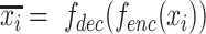, which includes two parts: an encoder 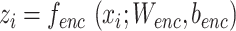, which generates the latent representations, and a decoder  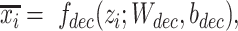which reconstructs original data from the latent representations. Here, represents the normalized gene expression of ith cell, is the low-dimensional embedding of and represents the recovered gene expression of ith cell, and are learnable parameters of encoder and decoder respectively, which will be learned in optimization. is further divided to two parts, and , which represent biological and noisy low-dimensional representations respectively. In the input layer, the expression value of every gene in each cell is rescaled to the range of [0,1] by subtracting minimum value and dividing the difference of maximum value and minimum value. The final layer performs sigmoid transformation to make the output within [0,1], whose output of ith cell is . The loss function of autoencoder is binary cross-entropy with the multiplication of the number of input genes :

(1)

Discriminator

The discriminator, is adversarially trained against encoder to ensure the feature distributions over different batches are as indistinguishable as possible in terms of batch labels, thus resulting in the batch-invariant representations. The input of discriminator is , the output is the probability of each batch label, which can be obtained by sigmoid transformation and softmax transformation for two batches and multiple batches respectively. Discriminator is used to encourage batch indistinguishability by an adversarial objective to minimize the distance (i.e. H-divergence (15)) between different batches. The empirical H-divergence for two-batches is,

(2)

Here, and represent two different batches, and and are the number of cells of batch and respectively., and represent biological low-dimensional representations of batch and batch respectively. is a hypothesis class, is a function with binary output and is an indicator function, whose output is 1 if condition is satisfied, otherwise is 0. H-divergence can be generalized to multiple batches if we use multiclass classifier for . However, it is hard to exactly compute , as it needs traversing all . Hence, we adopted the strategy ‘Proxy A-distance’ (15) to approximate . The ‘min’ part of equation (2) can be approximated by the classification loss of a classifier (discriminator) to discriminate different batches. Then the empirical H-divergence can be rewritten as:

(3)

where and are parameters of the classifier (discriminator). The classification loss adopts cross entropy as,

(4)

where is the output of the classifier : , is the batch label of ith cell, is the total number of cells and and are parameters of .

To encourage batch confusion and create the adversarial interactions between the feature extractor and discriminator, we train the encoder to minimize the empirical H-divergence between batches. Therefore, our goal is the following objective function:

(5)

where , are parameters of encoder. The object of equation (5) can be simplified as

(6)

To achieve minimization for and and maximization for and , gradient reversal layer (GRL) is introduced, whose output is the same as the input during forward propagation, and multiples by -1 during back propagation. That is to say, GRL basically performs the gradient ascent on feature extractor with respect to the discriminator loss. We replace with in as . The gradient reversal layer and new loss function of the discriminator are represented as,

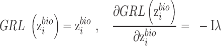(7)

(8)

The gradient reversal layer converts maximizing to minimizing in terms of and . is introduced to measure the degree of mixture of different batches. To avoid overcorrection, we assign th cell a weight , which is calculated from auxiliary classifier. So, the equation (8) can be further represented as

(9)

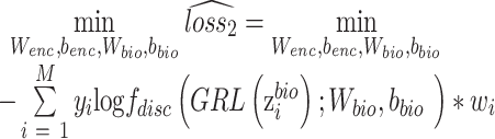
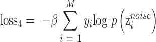
Auxiliary classifier

Auxiliary classifier is used to derive probability of a target-batch cell belonging to the source batch. This probability is used to weigh each cell in the batch-discriminator, making shared cells play a more important role on maximizing the discriminator. The weight is larger for cells from shared cell types. The input of auxiliary classifier is , and the output is the probability of batch labels. The loss function of auxiliary classifier is

(10)

where measures the importance of , and is the output of function : , whose parameters are and . To prevent the impact of minimizing the objective on , we introduce zero-gradient layer to , that is is replaced by . The zero-gradient layer is formulized as,

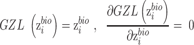(11)

According to the output of auxiliary classifier, we design a weight function as,

(12)

(13)

Where equation (12) for two batches and (13) for multiple batches.

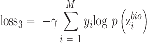
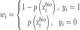
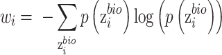
Noise classifier

Noise classifier is used to classify batch labels to obtain the low-representations of batch effect. The input of this classifier is and the output is the probability of batch labels. The loss function of this classifier is defined as

(14)

where , and is noise classifier's parameters to be learned and measures the importance of the noise classifier.

With the aforementioned derivation, we can formulate objectives of SCIDRL as follows:

(15)

We seek the parameters of encoder that maximize the loss of the discriminator (by making different batch distributions as indiscriminate as possible), while simultaneously seeking the parameters of the batch classifier that minimize the loss of the noise classifier.

Recovered gene expression

To obtain gene expression without batch effect, we set 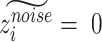for all cells. Then we concatenate and to obtain latent representations , whose batch effect are removed, and the recovered expressions without batch effect are obtained by .

Performance assessment

We compared the performance of our method SCIDRL with nine other methods on both simulated and recent scRNA-seq datasets with different types of batch effect (Supplementary Table S1). Their batch labels and cell types are known in advance, providing a golden standard. To evaluate the batch effect correction results of SCIDRL in comparison with other methods, we used Uniform Manifold Approximation and Projection (UMAP) visualizations together with four quantitative measures, including Local Inverse Simpson Index of batch (LISI-batch), Local Inverse Simpson Index of cell type (LISI-cell) (3), Comprehensive LISI (LISI-CoM) and Silhouette Score (SILS) (16).

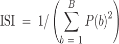
Local Inverse Simpson Index (LISI)

To measure the degree of batch mixing and biological signal preservation, we used LISI, which defines the effective number of datasets or cell types in a local neighborhood. It calculates the expected number of cells need to be sampled before one batch or one cell type is observed twice in a Gaussian kernel-based neighborhood. The Inverse Simpson Index is calculated as:

(16)

In which represents the total number of batches or cell types and represents the probability of batch or cell type in the local neighborhood. The local distribution is calculated as Gaussian kernel-based distribution with perplexity = 30. Specifically, the metric is defined as LISI-batch when using batch label, and LISI-cell when using cell type label. A better integration means a higher LISI-batch and a lower LISI-cell (or a higher 1/LISI-cell).

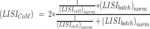
Comprehensive LISI (LISI-CoM)

To measure the degree of batch mixing and cell type purity simultaneously, we combined LISI-batch and 1/LISI-cell to obtain a new metric. Specifically, to eliminate the effect of different scales of these two metrics, both values are scaled to 0–1 by minmax scaling, which is

(17)

Then, the comprehensive LISI is defined as the harmonic mean of scaled LISI-batch and1/LISI-cell, which is

(18)

Silhouette SCORE (SILS)

To quantify the degree of mixture of batches and separation of different cell types, we adopted Silhouette Score (SILS), ranging from -1 to 1, as a synthetic index to measure how similar a cell is to its own cluster in comparison to other clusters.

(19)

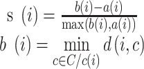
where represents the silhouette score of cell, is the average distance of the cell with all other cells in the cell type to which the cell belongs. For all other cell types , represents the average dissimilarity of the cell with all cells of cell type . A large value represents a good integration of different batches and separation of different cell types. For a fair comparison, we controlled the dimensions to be same in all methods when calculating SILS.

Datasets

We applied our method on thirteen types of datasets (Supplementary Table S1). These datasets contain both simulated datasets and recent public biological datasets. Each type of dataset includes two or more batches from different laboratories or tissues. Simulated datasets (simulated 1 and simulated 2): The simulated datasets are generated by Splatter (17), which devotes to simulate scRNA-seq data with drop out and batch effect using the zero-inflated negative binomial model. There are two types of simulated datasets: one type of dataset (simulated 1) contains 9500 cells with 500 genes from two batches. It covers six cell types and both batches have a rare cell type. The two batches have the same cell type compositions. The other type of dataset (simulated 2) also has two batches with the same number of cells and genes as the first dataset, which will be down-sampled to contain one shared cell type between two batches. For dataset with Group2 as shared cell type, there are one shared cell type (16.7%, which represents the percentage of the number of shared cell types against the total number of cell types). Pancreatic islet dataset (Pancreas): The pancreatic islet dataset contains 2,126 and 8,569 cells from two laboratories sequenced by CEL-Seq2 (18) and Drop-Seq technologies (referred to as ‘baron’ and ‘muraro’, respectively) (19), we marked the two batches as. It includes six rare cell types in both batches. There are eight shared cell types (53.3%). Human blood Dendritic Cells (DC) dataset: The DC dataset consists of 283 and 286 cells sequenced by Smart-Seq2 in two batches (20). There are two shared cell types between two batches (50%). Cell line dataset (Cell Line): The cell line dataset is composed of three batches, where batch 293T only contains 293T cells (2676 cells), batch Jurkat only contains Jurkat cells (3053 cells) and batch Mix contains both cell types (3162 cells) (7,21). The median of shared cell types between two batches is 50%. Mouse hematopoietic cells (Mouse Hemato) dataset: The mouse hematopoietic dataset includes two batches sequenced by Smart-Seq2 (1920 cells) (22) and Mars-Seq protocols (2927 cells) (23). There are three shared cell types (42.8%). Mouse retina dataset (Mouse Retina): The mouse retina dataset includes 44 808 and 27 499 cells from two laboratories using the Drop-seq technology (24,25). There are five shared cell types (38.5%). Mouse brain dataset (Mouse Brain): The mouse brain dataset contains 302 175 and 156 049 cells from two laboratories using Drop-seq (26) and SPLiT-seq protocols (27). There are nine shared cell types (64.2%). Mouse atlas dataset (Mouse Atlas): The mouse atlas dataset includes 21 855 and 13 320 cells sequenced by Microwell-Seq (28) and Smart-seq2 (29), respectively. These two batches have the same cell type compositions. Peripheral Blood Mononuclear Cells (PBMC) dataset: The PBMC dataset includes eighteen batches using nine scRNA-seq protocols. They have similar cell type compositions whereas varied cell amounts ranging from 526 to 6528 (30). The median of shared cell types between two batches is seven (82.6%). Mouse cortex dataset (Mouse Cortex): The mouse cortex dataset includes eight batches generated by Smart-seq2, DroNC-seq, 10× (v2) and sci-RNA-seq. All bathes have similar cell type compositions, and the numbers of cells are 644, 3130, 5571 and 5599 (30). The median of shared cell types between two batches is 3.5 (25%). Human cerebral organoids dataset (Human Cerebral Organoids): The human cerebral organoids dataset is consisted of 20 two-month human cerebral organoids from seven different ESC/iPSC lines in four batches, generated by 10× protocol. The number of cell types of four batches are 9, 10, 11 and 11 respectively. The cell amounts of four batches are 8581, 9433, 14 120 and 17 019, respectively (31). The median of shared cell types between two batches is 10.5 (91.3%). Eight-organ dataset (Eight Organ): the eight-organ dataset contains eight batches across three distinct sequencing technologies (i.e. Drop-seq, inDrops, 10x) from eight different organs, including the pancreatic islet, PBMC, kidney, liver, lung, spleen, and esophagus. The kidney dataset (32) contains 4487cells from allograft biopsy sequenced by InDrops, it includes several tubular cells, collecting duct cells (CD), immune cells, stromal cells and endothelial cells. The liver dataset contains 8476 cells from fresh hepatic tissues of five human livers sequenced by 10x platform. It includes hepatocytes, non-parenchymal cells and immune cells (33). The datasets of lung, spleen and esophagus contain 57 020, 94 257 and 87 947 cells, respectively. They are from 12 donors sequenced by 10× v3 (34). The lung dataset mainly contains ciliated cells, alveolar cells and immune cells. The spleen dataset has many immune cells and the esophagus dataset includes many epithelial cells. The median of shared cell types between two batches is four (20.6%).

The preprocessing of scRNA-seq datasets is performed by using the standard Seurat v3 pipeline. The input gene expression levels of each cell are first normalized to the same scale of 10⁴, which are followed by log transformation. We then use the ‘FindVariableFeatures’ of Seurat toolkit with ‘vst’ for parameter ‘method’ to select top 1000 highly variable genes (HVG) for each batch. We pool these genes to obtain the final HVG set for the following analysis.

RESULTS

We compared our method SCIDRL with nine other state-of-the-art methods. Considering the batch effect caused by different technologies, different laboratories and different organs, we used diverse simulated and biological datasets to testify the effectiveness of SCIDRL. In particular, we paid close attention to the following two aspects: datasets with rare cell types and datasets with different cell type compositions.

SCIDRL outperforms the state-of-art methods on simulated data

To assess the ability of SCIDRL on identifying rare cell types, we generated simulated dataset containing rare cell types. It is composed of two batches with five major cell types and one rare cell type (Group1). In this dataset, we generated one pair of highly similar cell types, Group1 and Group2 (Supplementary Figure S1A), which is used to testify the ability to avoid mixing similar cell types. We visualized the integration results of the two batches of one time in two-dimensional space so that the structure of data can be intuitively explored. Visualization of the originally uncorrected dataset shows that cells are separated due to batch effect and cell types (Figure 2A). The UMAP visualizations indicate only SCIDRL, Seurat v3, fastMNN, scanorama and scVI are able to remove batch effect and discern rare cell type Group1 (Figure 2A & Supplementary Figure S1B). Whereas, Liger, DESC and Harmony mistakenly mix up rare cell type Group1 and similar large cell type Group2. Moreover, iMAP fails to integrate Group1 from two batches. Bermuda not only mixes up Group1 and Group2 but fails to integrate the same cell types of two batches thoroughly (Supplementary Figure S1B). The quantitative results are indeed consistent with the intuitive visualizations (Figure 2B). The values of LISI-batch and 1/LISI-cell of SCIDRL are the highest among ten methods. The comprehensive metric of LISI-CoM shows that SCIDRL is the best method. In terms of comprehensive metric SILS, fastMNN is the best method, though all the other methods have good scores (SILS > 0.7), except for DESC, Bermuda, Harmony and liger. Overall, these results indicate that SCIDRL is tied as good method in integrating batch-shared rare cell types.

Figure 2.

Removing batch effect in simulated dataset. (A) Integration performance of SCIDRL for UMAP visualization on simulated 1 dataset with rare cell types. Each point represents a cell and the cell is colored according to its known cell type label and shaped according to batch label. (B) Performance comparison of ten integrated methods for four metrics (LISI-batch and 1/LISI-cell on the left, LISI-CoM and SILS on the right) on simulated 1 dataset. The x-axis represents LISI-batch or LISI-CoM and the y-axis represents 1/LISI-cell or SILS (larger value means better performance). Different colors represent different methods. (C) Integration performance of SCIDRL for UMAP visualization on down-sampled dataset with Group2 as the only shared cell type. Each point represents a cell and the cell is colored according to its known cell type label and shaped according to batch label. (D) Performance comparison of the ten integrated methods for four metrics (LISI-batch and 1/LISI-cell on the left, LISI-CoM and SILS on the right) on dataset with Group2 as the only shared cell type. The x-axis represents LISI-batch or LISI-CoM and the y-axis represents 1/LISI-cell or SILS. Different colors represent different methods.

To test the performance of SCIDRL in dataset with different cell type compositions, we generated another type of simulated dataset with two batches. This type of dataset is down-sampled to make sure there is only one shared cell type between the two batches. The UMAP visualizations of the down-sampled dataset, in which Group2 is the only shared cell type between two batches, are shown in Figure 2C and Supplementary Figure S1C, corresponding quantitative measurements of LISI-batch, 1/LISI-cell and SILS, LISI-CoM are displayed in Figure 2D. The intuitive visualizations indicate SCIDRL and fastMNN have the ability to achieve a better integration of Group2 and separation of different cell types, whereas other methods either can't remove batch effect of Group2 or mistakenly integrate Group2 with other cell types (Supplementary Figure S1C). Comparing the quantitative measurements LISI-batch and 1/LISI-cell, SCIDRL is still the top performing method in terms of batch integration and cell type purity. Similarly, SCIDRL is the top ranked method in comprehensive metric LISI-CoM. The SILS metrics of DESC, Seurat v3 and iMAP have high scores, however, they show a poor performance of batch mixing from the visualization results. If we down-sampled data to make the other cell type as the unique shared cell type between the two batches, the similar conclusion can be obtained (Supplementary Figure S1D–F). These results further indicate the high sensitivity and specificity of SCIDRL in datasets with rare cell types and datasets with different cell type compositions.

SCIDRL has competitive performance in two or three batches

To assess whether SCIDRL can integrate batch-shared rare cell types and preserve batch-specific rare cell types effectively, we applied it on human pancreatic islet dataset. Firstly, to assess whether SCIDRL can integrate scRNA-seq data with rare cell types, we used human pancreatic islet dataset. This dataset contains two batches from two laboratories, covering six rare cell types: 80 mesenchymal cells (0.7% of all cells); 55 macrophage cells (0.5%); 25 mast cells (0.2%); 19 epsilon cells (0.1%); 13 schwann cells (0.1%); 7 t cells (0.06%), which are labeled based on their marker genes: COL1A1, SDS, CPA3, GHRL, SOX10 (Supplementary Figure S2A). The epsilon cells are from two batches and the remaining rare cells are from one batch. The visualization results in Figure 3A and Supplementary Figure S2B show that only SCIDRL can effectively remove batch effect, clearly separate the batch-specific rare cell types and well mix batch-shared rare cell types. Seurat v3, scanorama and iMAP can effectively mix the epsilon cells across batches, but with the macrophage cells divided into different clusters. fastMNN has a good mixing of epsilon cells, but fails to separate schwann cells and mesenchymal cells, mast cells and macrophage cells. Whereas Harmony, Liger and scVI fail to mix the epsilon cells. Furthermore, Bermuda and DESC not only fail to mix the epsilon cells from different batches, but also mix different batch-specific rare cells. Comparing the scores of SILS (Supplementary Figure S2C) computed on rare cell types, SCIDRL has the top-five highest SILS. Comparing four metrics computed on all cells (Figure 3B), SCIDRL has the second highest LISI-batch and fourth highest 1/LISI-cell, highest LISI-CoM and third highest SILS, its average ranking of LISI-CoM and SILS is at the first place, which is congruent with UMAP visualizations. All these results proved the ability of SCIDRL in uncovering rare cell types.

Figure 3.

Removing batch effect in two or three batches. (A) Integration performance of SCIDRL for UMAP visualization on human pancreatic islet data. Each point represents a cell, in which rare cells are colored by different colors and other cells are colored by grey, the shape of each point represents batch label. (B) Performance comparison of the ten integrated methods for four metrics (LISI-batch and 1/LISI-cell on the left, LISI-CoM and SILS on the right) on pancreas dataset with all cells. The x-axis represents LISI-batch or LISI-CoM and the y-axis represents 1/LISI-cell or SILS. Different colors represent different methods. (C) Performance comparison of the ten integrated methods for four metrics (LISI-batch and 1/LISI-cell on the left, LISI-CoM and SILS on the right) on Cell Line (left), DC (middle) and Mouse Hematopoietic (right) datasets. The x-axis represents LISI-batch or LISI-CoM and the y-axis represents 1/LISI-cell or SILS. Different colors represent different methods. (D) Performance comparison of four methods (SCIDRL, Seurat v3, Liger and iMAP) on integrated and original gene expression pattern of epsilon's marker gene GHRL. Each point represents a cell and the cell is colored according to its expression value of GHRL.

To assess the integration ability on datasets with different cell type compositions, we applied it on DC, cell line and mouse hematopoietic datasets. The DC dataset contains four cell types, including CD1C, CD141, plasmacytoid DC (pDC) and double negative (DoubleNeg) cell types, with two batches contain two shared cell types (DoubleNeg and pDC). The cell line dataset consists of two cell types, with batch ‘293t’ is made up of 293t cells, batch ‘Jurkat’ contains Jurkat cells, batch ‘Mix’ contains both 293t cells and Jurkat cells. The mouse hematopoietic dataset covers six cell types, with two batches contain three shared cell types (CMP, GMP and MEP). For DC dataset, the UMAP visualizations (Supplementary Figure S2F) show that SCIDRL, Liger, Bermuda and Harmony successfully mixed the shared cell types (DoubleNeg and pDC), while separating CD1C and CD141 cells. Seurat v3, fastMNN, iMAP, scVI can achieve good separation of single CD141 and CD1C cells, but they bring CD1C and CD141 cells close, which would be hard to classify them as two cell types when the data is unlabeled. Scanorama incorrectly mixes up CD1C and CD141 cells. Bermuda and DESC not only mix up CD1C and CD141 cells but cannot integrate DoubleNeg or pDC. LISI-batch, 1/LISI-cell and LISI-CoM (Figure 3C) of SCIDRL are ranked third, second and first respectively, which further indicate the good performance of SCIDRL in DC dataset. For cell line dataset, from UMAP visualizations (Supplementary Figure S2G), we find that SCIDRL, Harmony, iMAP and DESC effectively integrate three batches while maintaining the cell type separation. Although Liger can achieve a good separation driven by cell types, some 293t cells and Jurkat cells are mistakenly mixed. Scanorama can mix 293t cells from different batches very well, but has poor batch mixing of the Jurkat cells. Seurat v3 has poor batch mixing of the 293T cells. BERMUDA fails to mix both 293t cells and Jurkat cells. FastMNN mixes up different cell types. From the LISI-batch metric, SCIDRL ranks the best one for batch integration. For the LISI-cell metric, SCIDRL, iMAP, Harmony and scanorama are the top methods in terms of cell type purity. For comprehensive metrics, SCIDRL has the highest LISI-CoM and relatively high SILS, which further indicate the good performance of SCIDRL in cell line dataset (Figure 3C). For mouse hematopoietic dataset, the UMAP visualizations (Supplementary Figure S2H) show that only SCIDRL, fastMNN and scanorama can not only remove batch effect but retain the independence of different cell types. Whereas Seurat v3, Liger, iMAP, scVI and DESC mix up different cell types such as GMP, CMP with LTHSC, LMPP. Bermuda and Harmony have poor batch mixing of three shared cell types (CMP, GMP and MEP). Comparing the quantitative results, SCIDRL is ranked first in two metrics (LISI-CoM, SILS) and second for LISI-batch and 1/LISI-cell (Figure 3C). We also tested SCIDRL on mouse brain, mouse retina and mouse atlas datasets. SCIDRL takes the first, third and sixth place for LISI-CoM respectively (Supplementary Figure S2I). On the whole, these results together suggest that SCIDRL is able to integrate datasets with different cell type compositions, especially datasets having a small number of shared cell types.

To assess the integration ability on datasets with different levels of similarity of cell type compositions, we down-sampled the original data to a varied number of shared cell types, ranging from one to eight shared cell types among two batches. For each level of similarity, we sampled different categories of cell types as the shared cell types to generate 57 groups. The comprehensive metrics LISI-CoM and SILS (Supplementary Figure S2D) show that SCIDRL achieves top-five performances for LISI-CoM and top-three performances for SILS. The average rankings of LISI-CoM and SILS of SCIDRL are at the first places for datasets having more than one shared cell types and the second place for dataset having one shared cell type. These results together suggest that SCIDRL is able to integrate datasets with different cell type compositions.

To investigate the impact of batch effect's removal on downstream analysis, we compared the pattern of marker genes identified from original data with from corrected data by SCIDRL, Seurat v3, Liger and iMAP. Other methods are not included because they operate on the low-dimensional representations instead of the corrected gene expression matrix. Here, we take the rare cell type as an example. Firstly, we checked the expression patterns of reported marker gene GHRL for epsilon cells (Figure 3D). Feature plot of GHRL in the original dataset reveals an obvious specific signal in epsilon cells, however, batch effect exists. SCIDRL and Seurat v3 inherits the information of marker gene from the original data with striking contrast and achieves batch effect removal. Whereas iMAP and Liger have high expression values of GHRL in many other cells, they do not preserve the same strong contrast in the marker gene. In the additional visualization results of rare cell types including mesenchymal, mast, schwann and rare beta cells which exhibit active endoplasmic reticulum (ER), the same performance of SCIDRL can be consistently observed (Supplementary Figure S2J). We also compared marker genes identified by original expression and corrected expression for all cells and epsilon cells (Supplementary Figure S2K). We compared the total overlaps among top N (N ranges from 1 to 100) marker genes identified in all cell types, SCIDRL, Liger and iMAP have similar overlaps and a bit less than Seurat v3. For the overlaps among the top N marker genes identified in epsilon cells, Seurat v3 has the highest degree of consistency, followed by SCIDRL and iMAP. These results together suggest that SCIDRL has a satisfactory performance on the recovery of marker genes after batch effect removal.

SCIDRL achieves effective integration of multiple batches

Next, we tested whether SCIDRL can integrate multiple batches. Firstly, we integrated dataset of human cerebral organoids from four batches with varied cell type compositions. The intuitive UMAP visualization results in Figure 4A and Supplementary Figure S3A show that SCIDRL, fastMNN, scanorama and scVI can remove batch effect and separate different cell states. Whereas Seurat v3, Harmony, Liger, iMAP and DESC mix up different cell types—cortical neural progenitor cells (NPCs), ganglion eminence (GE) NPCs and non-telencephalon NPCs. Bermuda has poor batch mixing of some cell types such as cortical NPCs. Among all methods, SCIDRL is top ranked in three metrics (LISI-batch, LISI-CoM, SILS) and second for 1/LISI-cell (Figure 4B). The quantitative measurements indicate the superior integration performance of SCIDRL in dataset with different cell type compositions.

Figure 4.

Removing batch effect in multiple batches. (A) Integration performance of SCIDRL for UMAP visualization on human cerebral organoid dataset. Each point represents a cell and the cell is colored according to its known cell type label and shaped according to its batch label. (B) Performance comparison of the ten integrated methods for four metrics (LISI-batch and 1/LISI-cell on the left, LISI-CoM and SILS on the right) on human cerebral organoid dataset. The x-axis represents LISI-batch or LISI-CoM and the y-axis represents 1/LISI-cell or SILS. Different colors represent different methods. (C) Integration performance of SCIDRL for UMAP visualization on PBMC dataset. Each point represents a cell and the cell is colored according to its known cell type label and shaped according to its batch label. (D) Performance comparison of the ten integrated methods for four metrics (LISI-batch and 1/LISI-cell on the left, LISI-CoM and SILS on the right) on PBMC dataset. The x-axis represents LISI-batch or LISI-CoM and the y-axis represents 1/LISI-cell or SILS. Different colors represent different methods. (E) Integration performance of SCIDRL for UMAP visualization on eight-organ dataset. Each point represents a cell and the cell is colored according to its known cell type label (left) and its batch label (right).

Then, we tested methods on nine publicly available datasets of human PBMC generated by 10x(v2), 10x(v3), CEL-Seq2, Smart-seq2, Seq-Well, inDrops and Drop-seq. The original nine datasets have similar cell compositions but varied cell quantities ranging from 526 to 6584. UMAP visualizations of all PBMC data in Figure 4C & Supplementary Figure S3B suggest SCIDRL, Harmony, Seurat v3, fastMNN and scanorama have ability to remove batch effect thoroughly while correctly merging cells from the same cell types. Liger also removes batch effect effectively but tends to split large cluster to smaller parts, for example megakaryocytes and CD4+ T cells are separated into two sub-clusters. The similar situation happens in scVI, which splits data into more fragments. Bermuda fails to integrate some CD4+ T cells, cytotoxic T cells or CD14+ monocytes. iMAP suffers from an over-correction problem, where T cells and monocytes are mistakenly mixed together. DESC is a poorer performer in integrating different batches. In terms of metric LISI-cell, harmony is the best method, though Seurat v3, scVI, scanorama, SCIDRL and fastMNN have similar good scores (1/LISI-cell > 0.75). SCIDRL is ranked second in two metrics (SILS and LISI-CoM) and third for LISI-batch (Figure 4D). Overall, SCIDRL ranks second considering the combination of LISI-CoM and SILS, which falls behind Seurat v3. In addition, we down sampled each dataset to have a smaller shared cell type number, zero or one among nine batches. The UMAP visualizations of dataset without shared cell types (Supplementary Figure S3C) show that SCIDRL, Harmony and scanorama are able to merge the same cell types and separate different cell types. Whereas, Seurat v3, Liger, Bermuda, and fastMNN mix up different cell types. Meanwhile, iMAP, scVI and DESC can’t remove batch effect of some shared cells. The quantitative measurements of LISI-CoM and SILS show that SCIDRL always ranks in the top two in dataset with none overlaps (Supplementary Figure S3E). For datasets containing CD14+ monocytes as shared cell type, UMAP visualizations (Supplementary Figure S3D) show that Bermuda, scanorama, scVI and DESC cannot remove batch effect for some techniques, whereas Seurat v3, Liger, iMAP and Harmony mix up CD14+ monocytes with other cell types. Only SCIDRL and fastMNN can integrate the shared cell type very well and reserve good cell type separation. The quantitative measurements show that SCIDRL is ranked second and third for SILS and LISI-CoM respectively, tied as the best method on the whole (Supplementary Figure S3E). We compared the marker genes detected before and after integration by SCIDRL, Seurat v3, Liger and iMAP on human cerebral organoids and PBMC datasets. Results show that all the methods have similar good performances (Supplementary Figure S3G).

To further demonstrate the effectiveness of SCIDRL, we additionally used a dataset, which contains four mouse cortex datasets sequenced by four scRNA-seq techniques. The quantitative measurements of original and down-sampled datasets, which contain astrocyte or endothelial cells as the only shared cell type, indicate SCIDRL still has consistent superior performance, ranking first or second combining SILS and LISI-CoM (Supplementary Figure S3F).

Joint analysis on cells across different organs is required in building human cell atlas. In such a scenario, biological variation is inevitably confounded by the differences between organs and experimental batches. Different organs share some common cell types such as immune cells, which may reveal segregation due to batch effect. We further evaluated whether SCIDRL can remove batch effect for cells that originate from various organs. We combined eight publicly available datasets from seven organs, including pancreas, PBMC, kidney, liver, lung, spleen, and esophagus. Normalized gene expression matrix of each dataset is obtained by dividing total reads to multiply 1, 000, 000 followed by taking logarithm. 500 Highly variable genes are selected for each dataset, then 1319 union of HVGs of each dataset are obtained for the following analysis. By the reason of exhausted computing resources when performing on Bermuda and calculating quantitative measures facing more than 200, 000 cells, we only compared nine methods by UMAP visualization and LISI metric. UMAP visualizations and quantitative measurements of original and integrated data obtained from SCIDRL and other eight methods are shown in Figure 4E, Supplementary Figure S3H & S3I. Except for pancreas and kidney, the rest of organs have abundant immune cells such as T cells, B cells, NK cells etc. We highlighted immune cells in UMAP spaces of original and integrated data colored by cell type labels and organ/batch labels (Supplementary Figure S3J). Compared with original data, except for DESC, these methods achieved efficient integrations of immune cells, which is also testified by higher LISI-batch of these methods than origin (Supplementary Figure S3I). Except for shared immune cell types, there are many organ-specific cell types. We displayed collecting duct (CD), loop of henle (LOH), proximal tubule (PT), distal tubule (DT) and pericyte of kidney, endothelial, hepatocyte and erythroid of liver, glands and epithelial of esophagus, alveolar, ciliated of lung, alpha, delta, epsilon etc. of pancreas (Supplementary Figure S3H). From the UMAP visualizations, only SCIDRL, scVI, fastMNN and scanorama can integrate the shared immune cells and reserve organ-specific cells, other methods mix up some kidney and pancreas cells with other organs, which are further indicated by the highest, relatively high and lower 1/LISI-cell of SCIDRL, scanorama and other methods.

Overall Performance of SCIDRL versus existing methods

To provide a convenient and intuitive summary of our results, we summarized the evaluation performance across four metrics on thirteen datasets and seven down-sampled datasets in Figure 5A–5D. Specifically, for each metric, each method was classified as ‘excellent’ (top 25%), ‘good’ (25–50%), ‘intermediate’ (50–75%) or ‘poor’ (75–100%). Methods were firstly ranked by their performances across the evaluation metrics. Then for each dataset, we categorized the methods into quantile buckets. For example, given ten methods, if one method lies below the first quantile (the top 25% of numbers, i.e. top three), this method should be encoded as ‘excellent’ (top 25%). With the LISI-batch metric, SCIDRL has ‘excellent’ performances on 10 datasets and ‘good’ performances on 4 datasets, ranking second (Figure 5A). Liger is slightly better than SCIDRL. Based on the LISI-cell metric, SCIDRL has ‘excellent’ performances on 12 datasets and ‘good’ performances on 6 datasets, ranking first (Figure 5B). For comprehensive metrics, SCIDRL has ‘excellent’ performances on 15 datasets for LISI-CoM (Figure 5C) and ‘excellent’ performances on 70% of 17 datasets for SILS (Figure 5D), whose comprehensive performance is best among ten methods. Though SCIDRL only has ‘intermediate’ performances on several datasets, it is a consistent performer. In general, SCIDRL performs the best based on these metrics.

Figure 5.

Overall Performance of SCIDRL versus existing methods. Performance categories of LISI-batch (A), 1/LISI-cell (B), LISI-CoM (C) and SILS (D) are displayed. The horizontal-axis represents different methods and the vertical-axis represents different datasets. Colored boxes represent method categories. Bermuda, Seurat V3 and scVI did not return values due to the memory limitation on large datasets. (E, F) The mean (E) and median (F) of the average rankings of LISI-CoM and SILS in four categories (‘LL’ represents little shared cells and little shared cell types, ‘LM’ represents little shared cells and many shared cell types, ‘ML’ represents many shared cells and little shared cell types, ‘MM’ represents many shared cells and many shared cell types). The x-axis represents different categories of dataset, the y-axis represents the mean or median of average rankings of LISI-CoM and SILS (smaller value means better performance). Different colors represent different methods.

To discuss the influence of the percentages of shared cells and shared cell types between two batches, we classified these datasets to four categories: little shared cells and little shared cell types (LL), little shared cells and many shared cell types (LM), many shared cells and little shared cell types (ML) and many shared cells and many shared cell types (MM). We take 50% as the threshold to classify dataset as ‘Little’ (L) when the percentage is lower than 50% and ‘Many’ (M) when the percentage is higher than 50%. We classified these datasets to four categories (Supplementary Table S2). We displayed the mean and median of average rankings of LISI-CoM and SILS among four categories for ten methods in Figure 5E and 5F, respectively. For LL, ML and MM, SCIDRL takes the first place, for LM, SCIDRL takes the third place, which further indicates the superiority of SCIDRL in datasets with different number of shared cells and shared cell types.

DISCUSSION

Removing batch effect is fundamental to the downstream analysis of scRNA-seq data. Recently, several methods have been developed to integrate scRNA-seq datasets from different sources. However, the major limitation is that most methods rely on identifying MNN pairs or clustering which may result in a loss of power and accuracy, especially for the datasets that have a small number of shared cell types or rare cell types.

To address these challenges, we introduce SCIDRL, which can disentangle biological meaningful (batch-invariant) representations from niose (batch-specific) representations without mannually finding MNN pairs or a preprocessed step of clustering. SCIDRL is achieved by jointly optimizing the low-dimensional representations in conjuction with training two competing classifiers operating on latent representations. It is an end-to-end method that can produce a corrected gene expression matrix for further downstream analysis such as the identification of marker genes or differential expression genes. Through extensive benchmark comparisons with nine common-used methods, the results demonstrate that SCIDRL is superior in most cases and achieves excellent performances for datasets with different cell type compositions and datasets with rare cell types. Although parameter tuning is an important issue for deep learning methods, we found in our experiment the default parameter is usually sufficient for achieving reasonable results for most analyses. To identify the best parameter for better integration, we proposed a quantitative heuristic strategy (Supplementary Figure S4). In addition, when integrating multiple batches, SCIDRL directly incorporate batch information in analysis, rather than based on pairwise integration, which Seurat v3, Liger, scanorama, fastMNN and iMAP usually do. In the process of pairwise integration, the order of batch corrected will affect the final results.

SCIDRL also has limitations. Since the design of SCIDRL to achieve disentanglement is based on classifier and discriminator, it can remove batch effect effectively for most cases. However, the classifier may not always perform well for highly unbalanced data (dataset with unbalanced number of cells of different batches), which can be solved by up-samplings or down-samplings. Another limitation is the running time for large datasets using a single GPU machine, which is a common issue for deep learning models. Fortunately, there have been many works including data parallelism (35), automatic selection of algorithm framework (36) and lightweight network design (37), etc., which can be applied in the future to accelerate the speed of SCIDRL.

As more scRNA-seq data become available, we believe SCIDRL will be a valuable tool for the comprehensive single cell heterogeneity analysis. This framework may be extended to integrate multimodal datasets such as scATAC-seq, spatial transcriptome etc., which is specially promising in future single cell multi-omics data analysis.

DATA AVAILABILITY

The code of SCIDRL is freely accessible online via https://github.com/guott15/SCIDRL.git.

Notes

Present address: Yang Chen, The State Key Laboratory of Medical Molecular Biology, Department of Molecular Biology and Biochemistry, Institute of Basic Medical Sciences, Chinese Academy of Medical Sciences, School of Basic Medicine, Peking Union Medical College, Beijing 100005, China.

SUPPLEMENTARY DATA

Supplementary Data are available at NAR Online.

FUNDING

National Key Research and Development Program [2018YFA0801402]; Natural Science Foundation of China [62050152,62003028, 81890991, 81890994]; Fundamental Research Funds for the Central Universities [2019RC045].

Conflict of interest statement. None declared.

REFERENCES

- 1. Rozenblatt-Rosen O., Stubbington M.J., Regev A., Teichmann S.A.. The human cell atlas: from vision to reality. Nature News. 2017; 550:451. [DOI] [PubMed] [Google Scholar]
- 2. Rozenblatt-Rosen O., Regev A., Oberdoerffer P., Nawy T., Hupalowska A., Rood J.E., Ashenberg O., Cerami E., Coffey R.J., Demir E.et al.. The Human Tumor Atlas Network: charting tumor transitions across space and time at single-cell resolution. Cell. 2020; 181:236–249. [DOI] [PMC free article] [PubMed] [Google Scholar]
- 3. Korsunsky I., Millard N., Fan J., Slowikowski K., Zhang F., Wei K., Baglaenko Y., Brenner M., Loh P., Raychaudhuri S.. Fast, sensitive and accurate integration of single-cell data with Harmony. Nat. Methods. 2019; 16:1289–1296. [DOI] [PMC free article] [PubMed] [Google Scholar]
- 4. Haghverdi L., Lun A.T., Morgan M.D., Marioni J.C.. Batch effects in single-cell RNA-sequencing data are corrected by matching mutual nearest neighbors. Nat. Biotechnol. 2018; 36:421–427. [DOI] [PMC free article] [PubMed] [Google Scholar]
- 5. Stuart T., Butler A., Hoffman P., Hafemeister C., Papalexi E., Mauck W.M. III, Hao Y., Stoeckius M., Smibert P., Satija R.. Comprehensive integration of single-cell data. Cell. 2019; 177:1888–1902. [DOI] [PMC free article] [PubMed] [Google Scholar]
- 6. Welch J.D., Kozareva V., Ferreira A., Vanderburg C., Martin C., Macosko E.Z.. Single-cell multi-omic integration compares and contrasts features of brain cell identity. Cell. 2019; 177:1873–1887. [DOI] [PMC free article] [PubMed] [Google Scholar]
- 7. Hie B., Bryson B., Berger B.. Efficient integration of heterogeneous single-cell transcriptomes using Scanorama. Nat. Biotechnol. 2019; 37:685–691. [DOI] [PMC free article] [PubMed] [Google Scholar]
- 8. Wang T., Johnson T.S., Shao W., Lu Z., Helm B.R., Zhang J., Huang K.. BERMUDA: a novel deep transfer learning method for single-cell RNA sequencing batch correction reveals hidden high-resolution cellular subtypes. Genome Biol. 2019; 20:165. [DOI] [PMC free article] [PubMed] [Google Scholar]
- 9. Wang D., Hou S., Zhang L., Wang X., Liu B., Zhang Z.. iMAP: integration of multiple single-cell datasets by adversarial paired transfer networks. Genome Biol. 2021; 22:63. [DOI] [PMC free article] [PubMed] [Google Scholar]
- 10. Lopez R., Regier J., Cole M.B., Jordan M.I., Yosef N.. Deep generative modeling for single-cell transcriptomics. Nat. Methods. 2018; 15:1053–1058. [DOI] [PMC free article] [PubMed] [Google Scholar]
- 11. Li X., Wang K., Lyu Y., Pan H., Zhang J., Stambolian D., Susztak K., Reilly M.P., Hu G., Li M.. Deep learning enables accurate clustering with batch effect removal in single-cell RNA-seq analysis. Nat. Commun. 2020; 11:2338. [DOI] [PMC free article] [PubMed] [Google Scholar]
- 12. Yang Y., Li G., Qian H., Wilhelmsen K.C., Shen Y., Li Y.. SMNN: batch effect correction for single-cell RNA-seq data via supervised mutual nearest neighbor detection. Brief. Bioinform. 2021; 22:bbaa097. [DOI] [PMC free article] [PubMed] [Google Scholar]
- 13. Ajakan H., Germain P., Larochelle H., Laviolette F., Marchand M.. Domain-adversarial neural networks. 2014; arXiv doi:09 February 2015, preprint: not peer reviewedhttps://arxiv.org/abs/1412.4446v2.
- 14. Cao Z., Ma L., Long M., Wang J.. Partial adversarial domain adaptation. Proceedings of the European Conference on Computer Vision (ECCV). 2018; 135–150. [Google Scholar]
- 15. Ganin Y., Ustinova E., Ajakan H., Germain P., Larochelle H., Laviolette F., Marchand M., Lempitsky V.. Domain-adversarial training of neural networks. J. Mach. Learn. Res. 2016; 17:2096–2030. [Google Scholar]
- 16. Rousseeuw P.J. Silhouettes: a graphical aid to the interpretation and validation of cluster analysis. J. Comput. Appl. Math. 1987; 20:53–65. [Google Scholar]
- 17. Zappia L., Phipson B., Oshlack A.. Splatter: simulation of single-cell RNA sequencing data. Genome Biol. 2017; 18:174. [DOI] [PMC free article] [PubMed] [Google Scholar]
- 18. Baron M., Veres A., Wolock S.L., Faust A.L., Gaujoux R., Vetere A., Ryu J.H., Wagner B.K., Orr S.S.S., Klein A.M.et al.. A single-cell transcriptomic map of the human and mouse pancreas reveals inter-and intra-cell population structure. Cell Syst. 2016; 3:346–360. [DOI] [PMC free article] [PubMed] [Google Scholar]
- 19. Muraro M.J., Dharmadhikari G., Grün D., Groen N., Dielen T., Jansen E., van Gurp L., Engelse M.A., Carlotti F., de Koning E.J.P.et al.. A single-cell transcriptome atlas of the human pancreas. Cell Syst. 2016; 3:385–394. [DOI] [PMC free article] [PubMed] [Google Scholar]
- 20. Villani A.C., Satija R., Reynolds G., Sarkizova S., Shekhar K., Fletcher J., Griesbeck M., Butler A., Zheng S., Lazo S.et al.. Single-cell RNA-seq reveals new types of human blood dendritic cells, monocytes, and progenitors. Science. 2017; 356:6335. [DOI] [PMC free article] [PubMed] [Google Scholar]
- 21. Zheng G.X., Terry J.M., Belgrader P., Ryvkin P., Bent Z.W., Wilson R., Ziraldo S.B., Wheeler T.D., McDermott G.P., Zhu J.et al.. Massively parallel digital transcriptional profiling of single cells. Nat. Commun. 2017; 8:14049. [DOI] [PMC free article] [PubMed] [Google Scholar]
- 22. Nestorowa S., Hamey F.K., Pijuan Sala B., Diamanti E., Shepherd M., Laurenti E., Wilson N.K., Kent D.G., Göttgens B.. A single-cell resolution map of mouse hematopoietic stem and progenitor cell differentiation. Blood. 2016; 128:e20–e31. [DOI] [PMC free article] [PubMed] [Google Scholar]
- 23. Paul F., Arkin Y.A., Giladi A., Jaitin D.A., Kenigsberg E., Keren-Shaul H., Winter D., Lara-Astiaso D., Gury M., Weiner A.et al.. Transcriptional heterogeneity and lineage commitment in myeloid progenitors. Cell. 2015; 163:1663–1677. [DOI] [PubMed] [Google Scholar]
- 24. Shekhar K., Lapan S.W., Whitney I.E., Tran N.M., Macosko E.Z., Kowalczyk M., Adiconis X., Levin J.Z., Nemesh J., Goldman M.et al.. Comprehensive classification of retinal bipolar neurons by single-cell transcriptomics. Cell. 2016; 166:1308–1323. [DOI] [PMC free article] [PubMed] [Google Scholar]
- 25. Macosko E.Z., Basu A., Satija R., Nemesh J., Shekhar K., Goldman M., Tirosh I., Bialas A.R., Kamitaki N., Martersteck E.M.et al.. Highly parallel genome-wide expression profiling of individual cells using nanoliter droplets. Cell. 2015; 161:1202–1214. [DOI] [PMC free article] [PubMed] [Google Scholar]
- 26. Saunders A., Macosko E.Z., Wysoker A., Goldman M., Krienen F.M., de Rivera H., Bien E., Baum M., Bortolin L., Wang S.et al.. Molecular diversity and specializations among the cells of the adult mouse brain. Cell. 2018; 174:1015–1030. [DOI] [PMC free article] [PubMed] [Google Scholar]
- 27. Rosenberg A.B., Roco C.M., Muscat R.A., Kuchina A., Sample P., Yao Z., Graybuck L.T., Peeler D.J., Mukherjee S., Chen W.et al.. Single-cell profiling of the developing mouse brain and spinal cord with split-pool barcoding. Science. 2018; 360:176–182. [DOI] [PMC free article] [PubMed] [Google Scholar]
- 28. Han X., Wang R., Zhou Y., Fei L., Sun H., Lai S., Saadatpour A., Zhou Z., Chen H., Ye F.et al.. Mapping the mouse cell atlas by microwell-seq. Cell. 2018; 172:1091–1107. [DOI] [PubMed] [Google Scholar]
- 29. Tabula Muris Consortium Single-cell transcriptomics of 20 mouse organs creates a Tabula Muris. Nature. 2018; 562:367–372. [DOI] [PMC free article] [PubMed] [Google Scholar]
- 30. Ding J., Adiconis X., Simmons S.K., Kowalczyk M.S., Hession C.C., Marjanovic N.D., Hughes T.K., Wadsworth M.H., Burks T., Nguyen L.T.et al.. Systematic comparative analysis of single cell RNA-sequencing methods. Nat. biotechnol. 2019; 38:737–746. [DOI] [PMC free article] [PubMed] [Google Scholar]
- 31. Kanton S., Boyle M.J., He Z., Santel M., Weigert A., Sanchís-Calleja F., Guijarro P., Sidow L., Fleck J.S., Han D.et al.. Organoid single-cell genomic atlas uncovers human-specific features of brain development. Nature. 2019; 574:418–422. [DOI] [PubMed] [Google Scholar]
- 32. Wu H., Malone A.F., Donnelly E.L., Kirita Y., Uchimura K., Ramakrishnan S.M., Gaut J.P., Humphreys B.D.. Single-cell transcriptomics of a human kidney allograft biopsy specimen defines a diverse inflammatory response. J. Am. Soc. Nephrol. 2018; 29:2069–2080. [DOI] [PMC free article] [PubMed] [Google Scholar]
- 33. MacParland S.A., Liu J.C., Ma X.Z., Innes B.T., Bartczak A.M., Gage B.K., Manuel J., Khuu N., Echeverri J., Linares I.et al.. Single cell RNA sequencing of human liver reveals distinct intrahepatic macrophage populations. Nat. Commun. 2018; 9:4383. [DOI] [PMC free article] [PubMed] [Google Scholar]
- 34. Madissoon E., Wilbrey-Clark A., Miragaia R.J., Saeb-Parsy K., Mahbubani K.T., Georgakopoulos N., Harding P., Polanski K., Huang N., Nowicki-Osuch K.et al.. scRNA-seq assessment of the human lung, spleen, and esophagus tissue stability after cold preservation. Genome Biol. 2020; 21:1. [DOI] [PMC free article] [PubMed] [Google Scholar]
- 35. Li M. Scaling distributed machine learning with system and algorithm co-design (Doctoral dissertation, PhD thesis, Intel). 2017; [Google Scholar]
- 36. Elsken T., Metzen J.H., Hutter F.. Neural architecture search: a survey. J. Mach. Learn. Res. 2019; 20:1997–2017. [Google Scholar]
- 37. Kozlov A., Andronov V., Gritsenko Y.. Lightweight network architecture for real-time action recognition. Proceedings of the 35th Annual ACM Symposium on Applied Computing. 2020; 2074–2080. [Google Scholar]
Associated Data
This section collects any data citations, data availability statements, or supplementary materials included in this article.
Supplementary Materials
Data Availability Statement