Removing independent noise in systems neuroscience data using DeepInterpolation

Abstract

Progress in many scientific disciplines is hindered by the presence of independent noise. Technologies for measuring neural activity—calcium imaging, extracellular electrophysiology, and fMRI—operate in domains in which independent noise (shot noise and/or thermal noise) can overwhelm physiological signals. Here, we introduce DeepInterpolation, a general-purpose denoising algorithm that trains a spatiotemporal nonlinear interpolation model using only raw noisy samples. Applying DeepInterpolation to two-photon calcium imaging data yielded up to 6 times more neuronal segments than in raw data with a 15-fold increase in single-pixel SNR, uncovering single-trial network dynamics that were previously obscured by noise. Extracellular electrophysiology recordings processed with DeepInterpolation contained 25% more high-quality spiking units than in raw data, while on fMRI datasets, DeepInterpolation produced a 1.6-fold increase in the SNR of individual voxels. Denoising was attained without sacrificing spatial or temporal resolution, and without access to ground truth training data. We anticipate that DeepInterpolation will provide similar benefits in other domains in which independent noise contaminates spatiotemporally structured datasets.

Introduction

Independent noise impacts experimental systems neuroscience, given the weakness of neuronal signals relative to the shot and thermal noise present in devices used for observing the brain. For example, in vivo imaging of fluorescent indicators (voltage and calcium) operates in photon-count regimes where shot noise dominates pixel-wise measurements. Similarly, thermal and shot noise present in electronic circuits can impact action potentials in in vivo electrophysiological recordings and BOLD responses in functional Magnetic Resonance Imaging (fMRI), impairing the measurement of authentic biological signals.

When datapoints in spatiotemporal proximity harbor the same underlying signal, but are independently affected by noise, median or Gaussian filters (in the time or Fourier domain) can be used to enhance single-trial dynamics, at the expense of reduced spatial and/or temporal resolution. Although this filtering approach is widely used, optimal denoising filters can be complicated to design by hand when data relationships span multiple dimensions (e.g., time and space) or are intrinsically non-linear.

Instead, it may be more efficient to remove noise by learning a model of the complex hierarchical relationships between data points, using a large training dataset¹. This approach would exploit statistical relationships between samples to reconstruct a noiseless version of the signal, rather than applying filters to remove noise. This approach has been successful for learning denoising or upsampling filters^2,3 but, until recently, was limited to cases where ground truth data is available. The Noise2Noise⁴ approach demonstrated that deep neural networks can be trained to perform image restoration without access to ground truth data, with performance comparable to training using cleaned data. Indeed, gradients derived from a loss function calculated on noisy samples are partially aligned towards the correct solution. Provided the noisy loss is an unbiased estimate of the true loss, the correct denoising filters are learned. However, unlike the data used to illustrate Noise2Noise⁴, neuronal data does not consist of pairs of samples with identical signals but different noise.

To overcome this limitation, we adopted an approach similar to the Noise2Self⁵ and Noise2Void⁶ frameworks. In the absence of training pairs, we solved an interpolation problem to learn the spatiotemporal relationships present in the data. We trained a model to learn the underlying relationship between each datapoint and its neighbors by optimizing the reconstruction loss calculated on each noisy instance of the sample itself. This approach is valid as long as the noise present in the target sample is independent from the input (adjacent) samples; otherwise, our relationship model would overfit the noise we seek to remove. We eliminated overfitting by omitting the target center frame from the input, and by presenting training samples only once during training. During inference, the dataset is streamed through the trained network to reconstruct a nearly noiseless version of the underlying signal.

We applied these principles to the problem of denoising dynamical signals at the heart of systems neuroscience, thereby building a general-purpose denoising algorithm we call DeepInterpolation. We describe and demonstrate the use of DeepInterpolation for two-photon in vivo Ca²⁺ imaging, in vivo electrophysiology, and whole brain fMRI. We anticipate that our approach will be applicable to other experimental fields with minimal modifications.

Results

Application of DeepInterpolation to two-photon Ca²⁺ imaging

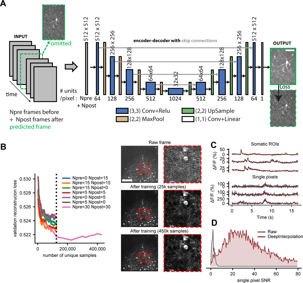
In our recordings of the mouse visual cortex, we first confirmed that our two-photon recordings with GCaMP6f were dominated by Poisson noise as shown by individual plots of all pixel variances against their means (Supplementary Fig. 1). Then, we constructed our denoising network with a UNet inspired architecture^8,9 following two simple principles: First, a single pixel can share information with pixels in a local region of the image (our neuronal network architecture had a final receptive field diameter of 78 pixels or 60 𝜇m), and second, the decay dynamics of calcium-dependent fluorescent indicators (GCaMP6f τ_peak = 80 ± 35 ms (s.e.m.); τ_1/2 = 400 ± 41 ms (s.e.m.)⁷) suggest “frames” (sets of simultaneously acquired 2D images) up to 1 second away can carry meaningful information.

We trained a neuronal network to reconstruct a center frame from the data present in N_pre prior and N_post subsequent frames. We omitted the center frame from the input to eliminate any information about the independent pixel-wise shot noise (Fig. 1A). We selected the final values of the meta-parameters (N_pre = 30 and N_post = 30) by comparing the validation loss during training (Fig. 1B, Supplementary Note).

Fig. 1 |. Training DeepInterpolation networks for denoising two-photon Ca²⁺ imaging.

(A) Schematic of an encoder-decoder deep network with skip connections for denoising two-photon imaging data. The encoder-decoder network utilized Npre and Npost frames, acquired at 30 Hz, before and after the target frame (labelled in green) to predict the central target frame (which was omitted from the input). Scale bar is 50 μm (B) Left: Validation loss shown as a function of unique samples for different combinations of (Npre, Npost) values during training for training a single network for the Ai93 reporter line (Methods). Y axis is the mean absolute difference between a predicted frame and a noisy sample across 2500 samples. Individual data samples were z-scored using a single estimate of mean and standard deviation per movie. Validation loss was therefore measured in normalized fluorescence units. Dashed vertical line indicates early stopping (due to the extreme computational demands during training) during evaluation of the parameter sets. Right: denoising performance of this model compared to a single raw frame (top) on a single representative experiment. Scale bar is 100 μm. Each red inset is 100 μm. (C) Six representative example traces extracted from a held-out denoised movie before (black) and after (red) denoising with DeepInterpolation. The top three traces are extracted from a somatic ROI, while the bottom three traces are extracted from a single pixel. (D) Distribution of SNR (mean over standard deviation, see Methods) for 10,000 pixels (randomly selected across N=19 denoised held-out test movies) before and after DeepInterpolation.

The Allen Brain Observatory datasets¹⁰ offered a large corpus of data for training of our denoising network: for each GCaMP6 reporter line (Ai93, Ai148), we had access to more than 100 million frames curated with standardized Quality Control (QC) metrics¹⁰. Within the limits of our computational infrastructure, we showed that using a larger number of both prior and subsequent frames as input yielded smaller validation reconstruction losses (Fig. 1B). Training required 225,000 samples pulled randomly from 1144 separate one-hour long experiments to stop improving (Fig. 1B). Since the loss is dominated by independent noise present in the target image, the reconstruction loss could not converge to zero. This was supported by simulating ideal reconstruction losses with known ground truth (Supplementary Fig. 2). In fact, even small improvement in the loss were associated with visible improvements in the reconstruction quality of the signal (Fig. 1B). At a typical frame rate of 30 Hz, a single hour of imaging yields 108,000 samples. Therefore, an average laboratory should have sufficient data to train their own DeepInterpolation network.

Applying this trained network to denoise held-out datasets yielded remarkable improvements in image quality (Supplementary Video 1, 2). The same trained network generalized well to additional examples (Supplementary Video 2). Shot noise was visibly eliminated from the reconstruction (Fig. 1C) while calcium dynamics were preserved, yielding a 15-fold increase in SNR (Fig. 1D, mean raw pixel SNR = 2.4 ± 0.01 s.e.m, mean pixel SNR after DeepInterpolation = 37.2 ± 0.2 s.e.m, N=9966 pixels). While the movies used during training were motion corrected, close inspection of the reconstructions showed that DeepInterpolation automatically removed small remaining motion artifacts (Supplementary Video 1, 2).

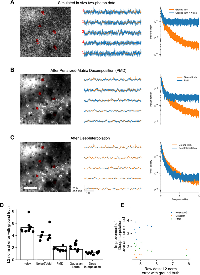
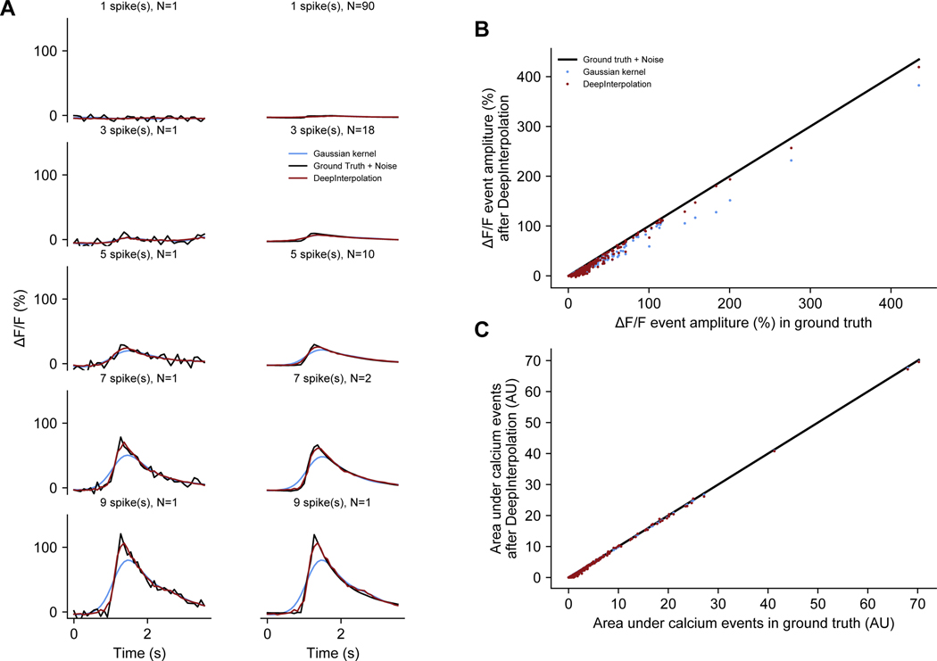
We compared our denoising approach to Penalized Matrix Decomposition (PMD)¹¹. While PMD properly reconstructed somatic activities, unlike DeepInterpolation, it rejected most of the variance present in background pixels (Supplementary Video 3). A key underlying assumption of PMD is the absence of motion artifacts. Contrary to what we saw after denoising with DeepInterpolation, we observed artifacts in movies denoised with PMD due to small residual motion artifacts (arrow in Supplementary Video 3). To compare these two approaches considering this limitation of PMD, we created simulated datasets devoid of motion artifacts, for which we had knowledge of the underlying ground truth signals, using the in silico Neural Anatomy and Optical Microscopy (NAOMi) approach¹². NAOMi combines a detailed anatomical model of a volume of tissue with models of light propagation and laser scanning to generate realistic Ca²⁺ imaging datasets (Extended Data Fig. 1, Supplementary Video 4). Because DeepInterpolation used information from nearby frames, it provided smoother calcium traces with reconstruction losses 1.4 to 2.3 times smaller than PMD (Extended Data Fig. 1). We confirmed that DeepInterpolation better rejected high frequency noise (Fourier transforms on Extended Data Fig. 1). We also compared DeepInterpolation with the pixel-wise approach of Noise2Void⁶, as well as with a temporal Gaussian kernel (Supplementary Video 5). As with PMD, the reconstruction error was 4 times higher with Noise2Void than with DeepInterpolation (Supplementary Fig. 3D). While the Gaussian kernel was effective at rejecting shot-noise, it heavily impacted the calcium event shape due to spatiotemporal smoothing effects (Extended Data Fig. 2). These results support the benefits of training more complex spatiotemporal models.

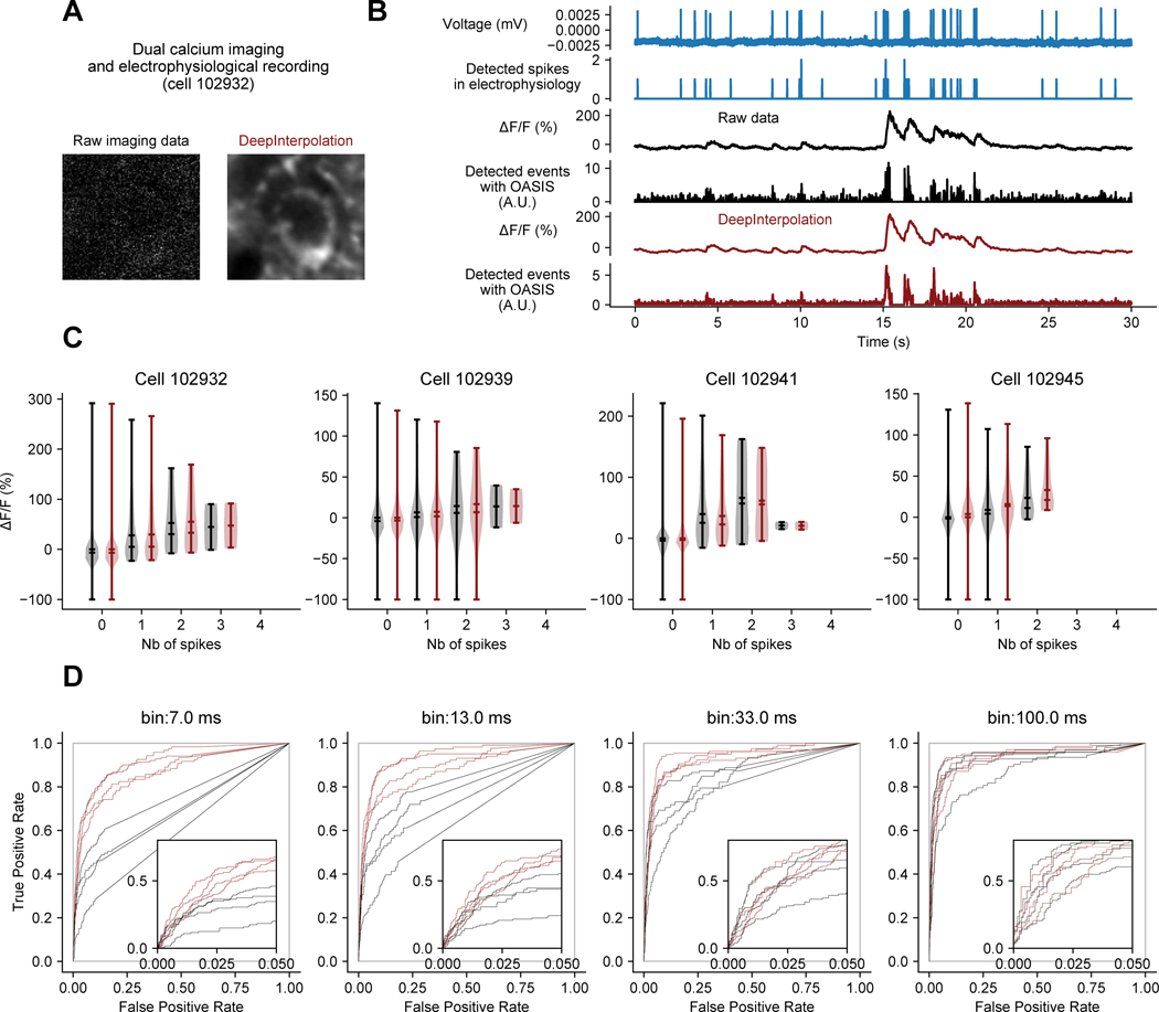
It was crucial to ensure that DeepInterpolation faithfully reconstruct calcium dynamics, without adding any spurious transients, as deep learning models are capable of “overinterpretation,” or enhancing features that do not actually exist¹³. To address this concern, we used our simulated data to compare individual reconstructed calcium transients to those in the ground truth dataset (Extended Data Fig. 2A). First, unlike after Gaussian smoothing, spike-triggered averages showed remarkable reconstruction of individual calcium transients, maintaining the peak amplitude and the area under the events (Extended Data Fig. 2B, C). Second, we leveraged an existing dataset in which both calcium activity and action potentials were recorded simultaneously from the same neurons (Extended Data Fig. 3A, B)¹⁴. The relationship between action potentials and calcium transients can be complex; therefore, we selected a subset of recordings performed in a Camk2a-tTA; tetO-GCaMP6s transgenic mouse where this relationship was strong (lower false positive rate in raw data). We found that DeepInterpolation did not alter the amplitude of calcium events associated with one or more action potential (Extended Data Fig. 3C). Furthermore, DeepInterpolation decreased the false positive rate of event detection, without affecting the hit rate (Extended Data Fig. 3D). Smaller bin sizes increased this effect (down to 7 ms for the original 150Hz sampling rate), demonstrating that DeepInterpolation can improve the temporal precision of spike inference.

DeepInterpolation transforms segmentation of active compartments

We next evaluated the impact of DeepInterpolation on the segmentation of neuronal compartments in movies of calcium activity. Existing approaches to segmentation rely on the analysis of correlation between pixels to create ROIs^15,16. After denoising, single-pixel pairwise correlations greatly increased from near-zero (average Pearson correlation = 9.0*10⁻⁴ ± 2.3*10⁻⁶ s.e.m, n = 4*10⁸ pairs of pixels across 4 experiments) to a significantly positive value (average Pearson correlation = 0.10 ± 1.210⁻⁵ s.e.m, n = 4*10⁸ pairs of pixels across 4 experiments, KS test comparing raw with DeepInterpolation: p = 9*10⁻⁷¹, n = 1,000 pixels randomly sub-selected, Supplementary Fig. 3). We expected that this increase in average correlation would improve the quality and the number of segmented regions. To that end, we tested its impact on segmentation algorithms from Suite2p¹⁶ and CaImAn¹⁷, two widely used calcium analysis packages.

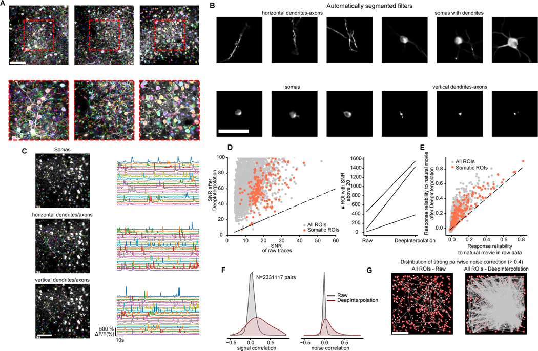
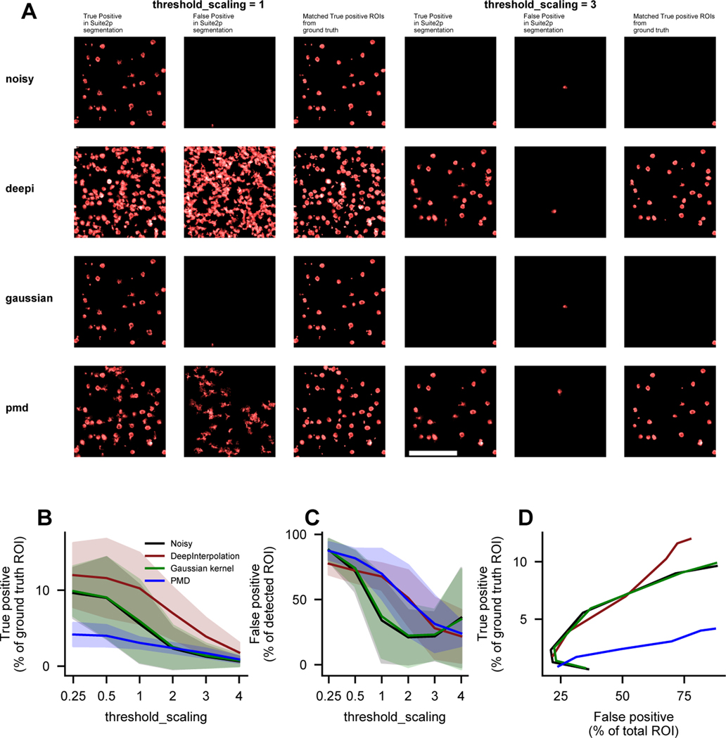
The improvement in correlation structure provided by DeepInterpolation benefited both algorithms. We first compared cell filters (images representing the weighted distribution of the compartments) with and without DeepInterpolation (Supplementary Fig. 4, 5). With Suite2p, higher-SNR neurons had identical filters while dimmer neuronal compartment showed better-defined filters with DeepInterpolation, sometimes recovering missing portions of the somas (Supplementary Fig. 4). DeepInterpolation had a similar impact on CaImAn (Supplementary Fig. 5). We leveraged synthetic datasets generated with NAOMi¹² to highlight the role of key segmentation parameters in weighting true positive and false positive rate of individual filters after DeepInterpolation (Extended Data Fig. 4). From real data, Suite2p extracted additional cell filters (Fig. 2A), sometimes encompassing dendrites or axons connected to a local soma, or even boutons attached to a horizontal dendrite (Fig. 2B). In some movies, smaller sections of axonal or dendritic compartments were detected, each with well-defined calcium transients (Fig. 2C). In future experiments, it might be helpful to acquire high-quality structural data to better define these small compartments.

Fig. 2 |. Applying DeepInterpolation to Ca²⁺ imaging reveals additional segmented ROIs and rich network physiology across small and large neuronal compartments.

(A) Three examples showing overlaid colored segmentation masks on top of a maximum projection image. Red dashed boxes show zoomed-in view. Scale bar is 100 μm. (B) Example individual weighted segmented filters showcasing dendrites, isolated somas, somas with attached dendrites, and axons and small sections of dendrites or axons. Scale bar is 50 μm (C) Manually sorted ROIs from one experiment showcasing the calcium traces extracted from each individual type of neuronal compartments (from top to bottom - cell body, horizontal processes, processes perpendicular to imaging plane). (D) Left: Quantification of SNR for all detected ROIs (gray dots) and somatic ROIs (red dots) with and without DeepInterpolation. Dashed line represents the identity line. Right: Comparison of the number of ROIs with an SNR above 20 with and without DeepInterpolation. Each line is a single experiment (n = 3 experiments). (E) Quantification of the response reliability of individual ROIs across 10 trials of a natural movie visual stimulus. Dashed line represents the identity line. (F) Left: signal correlation (average correlation coefficient between the average temporal response of a pair of neurons) for all pairs of ROI in (D) for both raw and denoised traces. Right: noise correlation (average correlation coefficient at all time points of the mean-subtracted temporal response of a pair of neurons) for all pairs of ROIs in (D). (G) For an example experiment, pairs of ROIs with high noise correlation (>0.4) are connected with a straight line for both original two-photon data and after DeepInterpolation. Scale bar is 100 μm.

Although some compartments were not detected in the original raw movie, we applied the weighted masks to both denoised and raw movies to quantify the improvement in SNR of the associated temporal trace. ROIs associated with somatic compartments typically yielded a mean SNR of 21.0 ± 0.5 (s.e.m, n = 240 in 3 experiment) in the original movie (Fig. 2D); after denoising, most of those ROIs had an SNR above 40 (mean 73.8 ± 0.5 s.e.m). Similarly, the mean SNR across all compartments, including the smallest apical dendrites, went from a mean of 13.2 ± 0.1 s.e.m (n = 3385 in 3 experiments) to 73.8 ± 0.5 s.e.m. To detect a calcium rise of about 10%, an SNR above 20 is necessary for those events to be twice as large as the noise. This suggests that removing shot noise may increase our capability to detect the presence of single spikes. Detecting single spikes remains difficult owing to the complexity of the relationship between calcium levels and action potentials^14,19, which is unrelated to the presence of independent noise. Nonetheless, the average number of detected active ROIs with SNR above 20 went from 178 ± 135 (s.e.m., in 3 experiments) to 1122 ± 371 in a 400×400 um² field of view (Fig. 2D) – i.e. six times more neuronal compartments became available for analysis from a single movie following DeepInterpolation,.

DeepInterpolation improves the analysis of correlated activity

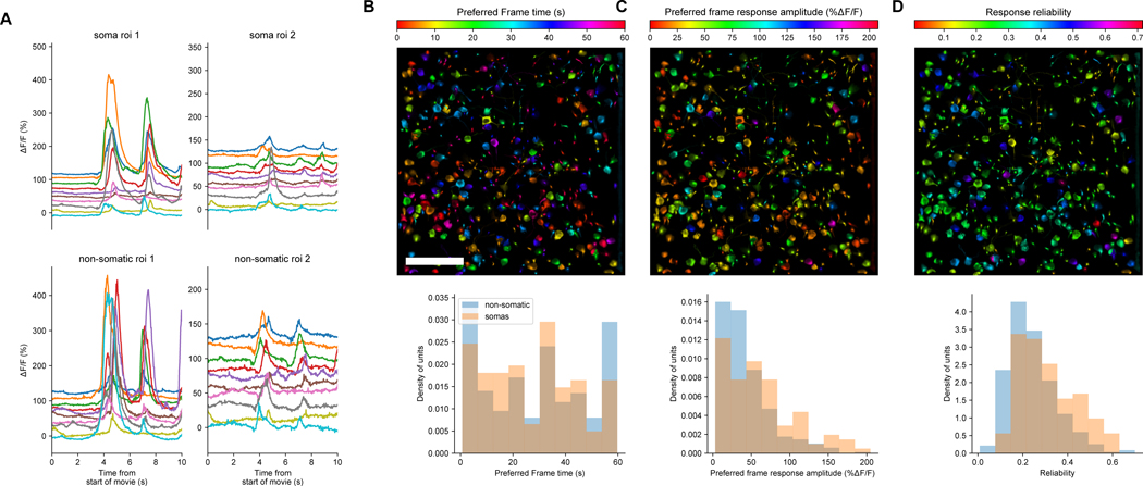
We next analyzed the response of all segmented compartments to 10 repeats of a natural movie presentation. We found examples of both large and small responses to natural movies in somatic and non-somatic compartments (Extended Data Fig. 5). The trial-by-trial response reliability increased substantially from raw traces to traces after DeepInterpolation (Fig. 2E), both for somatic ROIs (raw: mean 0.10 ± 0.01, DeepInterpolation: mean 0.20 ± 0.01; s.e.m, n = 240 ROIs in n = 3 experiments) and across all ROIs (raw: mean 0.029 ± 0.001, DeepInterpolation: mean 0.113 ± 0.002; s.e.m, n = 3385 ROIs in n = 3 experiments).

Neuronal representations are inherently noisy. This property of neuronal networks has fueled studies on the relationship between the average signal representation in individual neurons and the trial-by-trial fluctuation of their responses^20–22. Experimental noise impacts this measure of neuronal relationships as it modulates trial-by-trial responses. For each pair of ROIs in a single experiment, we extracted their shared signal and noise correlation. As expected, we found that both signal and noise correlation increased after denoising (signal: from 0.06725 ± 0.00006 s.e.m to 0.25 ± 0.0001 s.e.m; noise from 0.02240 ± 0.00002 s.e.m to 0.12351 ± 0.00008 s.e.m; both for 2,329,554 pairs of ROIs from three experiments; Fig. 2F). This result was not just due to the improved segmentation as it was preserved using ROIs only detected on raw noisy data (Supplementary Fig. 6). To further illustrate how these improved measures of neuronal fluctuations impacted the analysis of functional interactions, we compared the spatial distribution of pairwise correlations between neurons during natural movie presentation. DeepInterpolation largely increased the number of strong pairwise interactions for both somatic and non-somatic pairs (Fig. 2G, all ROIs: 43 to 1721 pairs), including pairs of ROIs much further apart than our DeepInterpolation model’s receptive field of 60 μm.

Fine-tuning generalizes pre-trained models to previously unseen datasets

How well will this approach scale beyond the highly standardized datasets we have analyzed so far? We originally aggregated training data across hundreds of experiments to generate a few DeepInterpolation networks that could generalize across different recording conditions. These broadly trained models should be a good starting point for fine-tuning on other datasets, provided that individual frames of the data can fit within our 512 by 512 window, with unoccupied pixels filled with zero values.

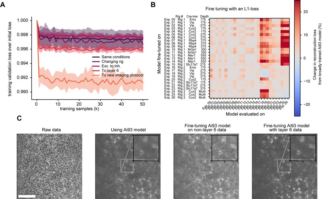
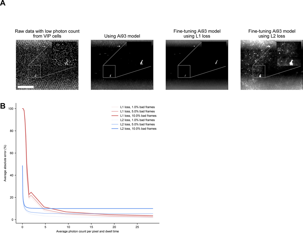
To test this, we selected 26 datasets collected with both different and shared experimental conditions: one subset included mice with labelled inhibitory neurons instead of excitatory neurons; another subset was collected using a different model of microscope; and a final set used an imaging frame rate of 10 Hz (instead of 30 Hz). For each experiment, we fine-tuned our pretrained model using 50,000 random frames. In all cases, training converged after 20,000 frames (Fig. 3A). When evaluating the performance of all 26 models on all pairwise movie combinations, we found that fine-tuned models had improved reconstruction performance at the expense of generalization across experimental conditions (Fig. 3B). We applied DeepInterpolation to recordings from neurons in cortical Layer 6, which have higher levels of background fluorescence than recordings from more superficial layers (Fig. 3C). The improvements were especially visible in the reconstruction of the background (Fig 3C, Supplementary Video 6). When fine-tuning for low SNR experiments (below 5 photons per pixel per dwell time), we found that an L1 loss could cause abnormally damped fluorescence values (Extended Data Fig. 6). While L1 loss forces training to converge toward the median of all potential outcomes, providing resilience to artifactual frames, like motion artifacts, it discards the most meaningful output frames at low photon count. In this case, fine-tuning with an L2 loss, which converges toward the mean of all potential outcomes, recovered denoising performances with low photon counts experiments (Extended Data Fig. 6, Supplementary Video 7).

Fig. 3 |. Fine-tuning pre-trained DeepInterpolation models recover reconstruction performance with minimal training data.

(A) Training reconstruction loss in validation data throughout fine-tuning a pre-trained model (Ai93 DeepInterpolation model) on previously unseen two-photon calcium movies. For training, experimental conditions differed as follows: switching to a different experimental rig with the same recording conditions (Changing rig), using data from inhibitory neurons (Exc. to inh.) recorded with a different reporter line (Ai148), using data from layer 6 (To layer 6) recorded with an Ntsr1-Cre_GN220;Ai148 mouse line, using data from the same mouse line but imaged at 10Hz (instead of 30Hz) and performing volume scanning with a piezo objective scanner (To new imaging protocol). Dashed lines represent the standard deviation across rounds of training with similar conditions. (B) Cross-model evaluation performance when varying the recording conditions. The broadly trained Ai93 DeepInterpolation model was fine-tuned separately on 26 recording experiments with varying imaging conditions. We then evaluated each fine-tuned model on all 26 experiments separately to plot the cross-condition reconstruction performance. The performance was normalized to the broadly trained Ai93 model. (C) Comparison of an example raw frame recorded with an Ntsr1-Cre_GN220;Ai148 mouse line in the layer 6 (left) with its corresponding frame after DeepInterpolation with various models. First, we used a broadly pre-trained Ai93 model, then a fine-tuned model on non-layer 6 data and finally a model trained on the same exact layer 6 experiment. Scale bar is 100 μm.

Application to electrophysiological recordings

Electrophysiological recordings from high-density silicon probes have similar characteristics to two-photon imaging movies: information is shared across nearby pixels (electrodes), as well as across time. Thus, a similar architecture should perform well for denoising electrophysiology data, in particular for removing strictly independent thermal and shot noise from the recordings.

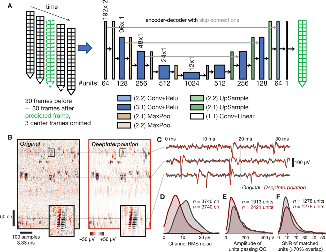
Because a single action potential lasts ~1 ms, we constructed our interpolating network to predict the voltage profile at any given moment from 30 preceding and 30 following datapoints acquired at 30 kHz. Unlike for two-photon imaging, we found that omitting one sample before and after the center sample better rejected the background noise while maximizing the signal reconstruction quality. The architecture of the network was like the one used for two-photon imaging, except that we reshaped the input layer to match the approximate layout of the Neuropixels recording sites (Fig. 4A). Because electrophysiological recordings have a 1,000-fold higher sampling rate than two-photon imaging, we trained the network on just 3 experiments in total²³.

Fig. 4 |. Applying DeepInterpolation to electrophysiological recordings decreases background noise and yields additional detected neuronal units.

(A) Structure of the DeepInterpolation encoder-decoder network for electrophysiological data recorded from a Neuropixels silicon probe, with two columns of 192 electrodes each, spaced 20 μm apart. Data is acquired at 30 kHz. (B) Side-by-side comparison of original (left) and denoised (right) data, plotted as a 2D heatmap with time on the horizontal axis and channels along the vertical axis. Insets show a close-up of a single action potential across 22 contiguous channels (the box is 3.6 ms wide). (C) Denoised time series (red) overlaid on the original time series (gray) for three channels from panel B. (D) Histogram of RMS noise for all channels from 10 experiments, before and after applying DeepInterpolation. (E) Histogram of waveform amplitudes for all high-quality units from 10 experiments. (F) Histogram of waveform SNRs for all units that were matched before and after denoising.

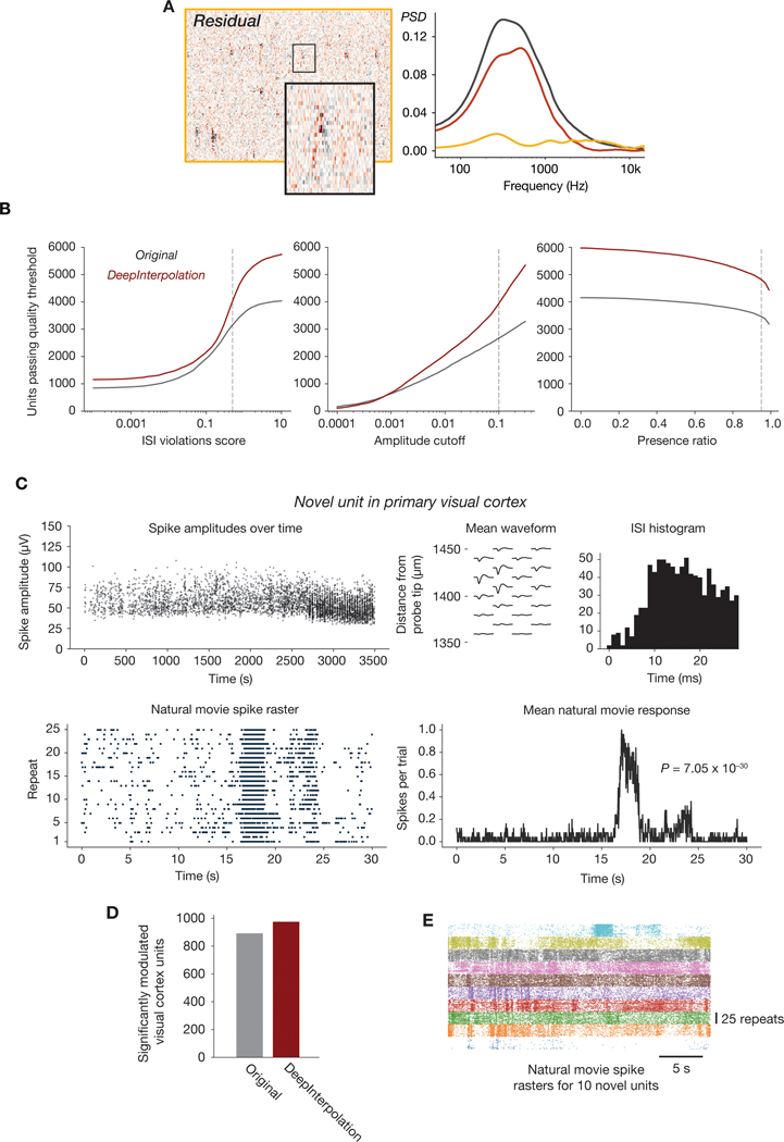
After inference, a qualitative inspection of the recordings showcased excellent noise rejection (Fig. 4B). We compared spike profiles before and after denoising and found more clearly visible spike waveforms in the denoised data, especially for units of lower amplitude (Fig. 4B, inset; Fig. 4C). The residual of our reconstruction showed weak spike structure but spectral analysis revealed a mostly flat frequency distribution (Extended Data Fig. 7A). The overall shape (amplitude and decay time) of individual action potentials was preserved, while the median channel RMS noise was decreased 1.7-fold (6.96 μV after denoising, Fig. 4D). After denoising and spike sorting, we found 25.5 ± 14.5% s.d more high-quality units per probe (ISI violations score < 0.5, amplitude cutoff < 0.1, presence ratio > 0.95). The number of detected units was higher after DeepInterpolation regardless of the chosen quality metric thresholds (Extended Data Fig. 7B). Most additional units had low-amplitude waveforms, with the number of units with amplitudes above 75 μV remaining roughly the same (1532 before vs. 1511 after), while the number with amplitudes below 75 μV increased (381 before vs. 910 after) (Fig. 4E). For units that were matched before and after denoising (at least 70% overlapping spikes), average SNR increased from 11.2 to 14.5 (Fig. 4F).

By searching for spatiotemporally overlapping spikes, we determined that 6.2 ± 2.9% s.d. of units in the original recording were no longer detected after DeepInterpolation (<50% matching spikes). However, this was counterbalanced by the addition of 20.2 ± 4.8% s.d. units that had fewer than 50% matching spikes in the original data (Extended Data Fig. 7C). This is less than the 25.5% increase cited above, because it accounts for a minority of units that were detected but merged in the original data. To validate that these additional units were likely to correspond to actual neuronal compartments, we analyzed their responses to natural movies, using the same movie as in the two-photon imaging study. We found approximately 9% more reliably visually modulated units in the visual cortex after denoising (Extended Data Fig. 7D) and found examples of stimulus-modulated units that were previously undetected (Extended Data Fig. 7E). These results showcase the ability of DeepInterpolation to reveal additional biologically relevant information about the neuronal circuits under investigation.

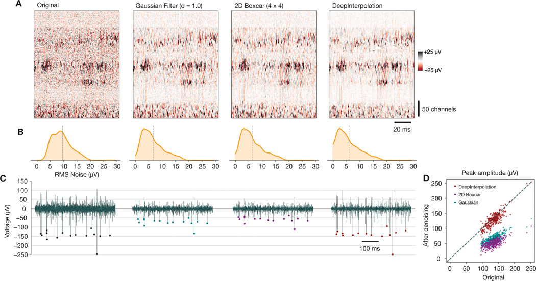
We compared the impact of DeepInterpolation on our electrophysiology data to that of two much simpler denoising methods, smoothing with a Gaussian or boxcar window (Extended Data Fig. 8A). Both simpler methods were able to reduce RMS noise levels to a range consistent to that achieved by DeepInterpolation (Extended Data Fig. 8B). However, this came at the expense of spike amplitude attenuation (Extended Data Fig. 8C,D).

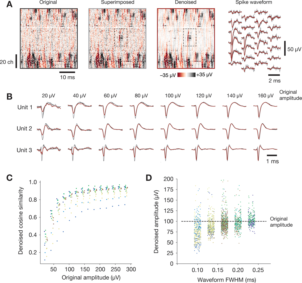
In order to determine the conditions under which DeepInterpolation can preserve spike waveform shape, we applied it to a simulated ground truth dataset where spikes were superimposed at random locations in the original data (Extended Data Fig. 9). For most waveforms and amplitudes, waveform shape was preserved after applying DeepInterpolation. However, we did observe some attenuation at low amplitudes and for narrow waveforms (FWHM < 0.15 ms). Reduced similarity is expected at low amplitudes, where noise fluctuations can cause distortions in waveform shape. Future iterations of the DeepInterpolation approach could mitigate this by using a similarity metric for narrow spike waveforms in simulated ground truth datasets to iterate the network architecture.

Application to functional Magnetic Resonance Imaging (fMRI)

We evaluated if DeepInterpolation could aid the analysis of volumetric datasets like fMRI. fMRI is very noisy, as the BOLD response is typically just a 1–2 % change of the total signal amplitude²⁵. Thermal noise is present in the electrical circuit receiving the MR signal. A typical fMRI processing pipeline involves averaging nearby pixels and successive trials to increase the SNR^26,27. Thus, our approach could replace smoothing kernels with more optimal local interpolation functions, without sacrificing spatial or temporal resolution.

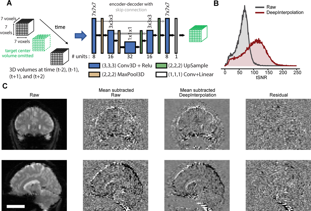
Given the lower spatiotemporal sampling rate of fMRI, we trained a more local interpolation function with only 2 pooling layers. To reconstruct the value of a brain sub-volume, we fed a neural network with a consecutive temporal series of a local volume of 7 × 7 × 7 voxels. We omitted the entire target volume from the input (Fig. 5A). We trained a single denoising network using 140 fMRI datasets acquired across 5 subjects, comprising 1.2 billion samples in total.

Fig. 5 |. Applying DeepInterpolation to fMRI removes thermal noise.

(A) Structure of the DeepInterpolation encoder-decoder network for fMRI data. Instead of predicting a whole brain volume at once, the network reconstructs a local 7×7×7 cube of voxels. (B) tSNR for 10,000 voxels randomly distributed in the brain volume in raw data and after DeepInterpolation. (C) Exemplar reconstruction of a single fMRI volume. First row is a coronal section while the second row is a sagittal section through a human brain. In the second column, the temporal mean of 3D scan was removed to better illustrate the presence of thermal noise in the raw data. The local denoising network was processed throughout the whole 3D scan for denoising. The impact of DeepInterpolation on thermal noise is illustrated in the 3rd column. The 4th column shows the residual of the denoising process. Scale bar is 5 cm.

We extracted the temporal traces from individual voxels and found that SNR increased from 61.6 ± 20.6 s.d. to 100.40 ± 38.7 s.d. (n = 100,001 voxels) (Fig. 5B). Applying the trained network to held-out test data resulted in excellent denoising performance (Fig. 5C). We noticed that the background noise around the subject’s head was excluded and only present in the residual image (Fig. 5C, Supplementary Video 8). Surrounding soft tissues became visible after denoising (Fig. 5C, Raw data: background voxel std = 7.59 ± 0.01 s.e.m; brain voxels std = 15.95 ± 0.08 s.e.m., n = 10,000 voxels; DeepInterpolation data: background std = 2.24 ± 0.01 s.em., n = 10,000; brain voxels std = 9.72 ± 0.05 s.e.m., n = 10,000 voxels; Residual: background std = 7.91 ± 0.01; brain voxels std = 15.79 ± 0.08, n = 10,000 voxels). We compared movies extracted with DeepInterpolation to fully pre-processed movies smoothed with a Gaussian denoising kernel (Supplementary Video 9): the original 3D resolution was fully maintained in DeepInterpolation while the processed data with Gaussian kernel diffused dynamics across nearby voxels. The residual movie showed no visible structure except for occasional blood vessels, corrected motion artifacts and head mounting hardware (Fig. 5C, Supplementary Video 10).

Discussion

We have presented DeepInterpolation, which can reconstruct nearly noiseless versions of datasets without the need for ground truth training data. Applying DeepInterpolation to Ca²⁺ imaging, electrophysiological recordings, and fMRI demonstrates its widespread benefits and ability to uncover previously hidden neuronal dynamics. While our approach is closely related to Noise2Self⁵ and Noise2Void⁶, we developed our framework independently. As a result, several key differences are notable. First, instead of working with single fluorescence frames with pixel-wise omissions, we adapted our approach to the types of complex multi-dimensional biological datasets at the heart of systems neuroscience. Second, we trained our models on large databases, demonstrating the impact of richer denoising models on existing neuroscience data and on workflows such as cell segmentations or spike sorting. Third, we contributed practical solutions to relevant problems in this domain: we provide a network topology that works on real neuroscience datasets, a training regimen that requires data volumes that are available to most laboratories, and a fine-tuning process to adapt pre-trained models to new datasets.

We anticipate that DeepInterpolation will enhance post-processing steps that can leverage higher SNR levels and more pronounced correlation structure. For instance, background correction in two-photon imaging data relies on measurements of the contamination from neighboring pixels. Typically, measurement within background pixels are less reliable than in somatic pixels, given the lower expression-level in the background, necessitating the averaging of distant pixels. With fewer, more local neighboring pixels needed to make this measurement, we expect background correction reliability to increase.

We anticipate DeepInterpolation to become instrumental for the advancement of large-scale voltage imaging of neuronal activity^28,29 and to facilitate practical application of high-speed fMRI, which currently operates in a regime in which thermal noise dominates the BOLD signal. Our approach should permit scientists in a variety of fields to re-analyze their existing datasets, but with independent noise reduced or removed.

Methods

Description of experimental data used in this study

All experimental datasets used in this study were previously collected and published separately. Associated datasets were all made available online. Animal and human work approval was described in each associated publication.

We trained 4 denoising neuronal networks in this study: one for two-photon imaging experiments using the Ai93(TITL-GCaMP6f) reporter line, one for the Ai148(TIT2L-GCaMP6f-ICL-tTA2) reporter line^30,31, one for Neuropixels recordings using “Phase 3a” probes³², and one for fMRI imaging using datasets from a study published on OpenNeuro.org³³. For Neuropixels, training data consisted of 1-hour of segments extracted from 10 different ~2.5 hour long recordings (see below for information on the specific sessions used). For fMRI, the dataset contained fMRI data from five subjects with 3 types of scanning sessions: “ses-perceptionTraining”, “ses-perceptionTest” and “ses-imageryTest”. We trained our denoiser on “ses-perceptionTraining” sessions and measured the denoising performance on “ses-perceptionTest” sessions.

All raw datasets used for training are available at the time of publication through AWS S3 buckets (Amazon.com, Inc., https://openneuro.org/datasets/ds001246/versions/1.2.1 and https://registry.opendata.aws/allen-brain-observatory/).

Pre-processing steps

Two-photon imaging movies were motion-corrected similarly to our previous publication¹⁰. The motion correction algorithm relied on phase correlation and only corrected for rigid translational errors. We used these motion-corrected movies for denoising. All motion corrected movies were used directly as is during training, we did not exclude any frames or recordings due to motion instabilities. SNR was not used as a criteria for inclusion and was highly variable in the training set as we usually set laser power to the maximum level safely tolerated by the tissue¹⁰. Potential motion correction errors occasionally present in our data were typically below neuronal soma size. We did not re-apply motion correction after DeepInterpolation.

For Neuropixels recordings, the median across channels was subtracted to remove common-mode noise. The median was calculated across channels that were sampled simultaneously, leaving out adjacent channels that are likely measuring the same spike waveforms, as well as reference channels that contain no signal. For each sample, the median value of channels N:24:384, where N = [1,2,3,…,24], was calculated, and this value was subtracted from the same set of channels. Importantly, this step removes noise that is correlated across channels, without affecting the independent noise targeted by DeepInterpolation. We performed denoising on the spike band after the median subtraction and offline filtering steps (150 Hz high pass) were applied.

For fMRI recordings, we used raw, unprocessed Nifti-1 volume data provided on OpenNeuro.org (https://openneuro.org/datasets/ds001246/versions/1.2.1). We compared denoised fMRI recordings with processed datasets available on OpenNeuro.org that included a Gaussian kernel. The Gaussian kernel was part of a standard fMRI processing pipeline using SPM5 (http://www.fil.ion.ucl.ac.uk/spm) and introduced as part of a motion correction algorithm. We did not alter the parameters of this gaussian kernel.

Detection of ROIs in two-photon data

We used two different segmentation algorithms in this study. The first one was described in a previous publication and leverages a succession of morphological filters to extract binary masks surrounding active pixels¹⁰. These masks are publicly available through the AllenSDK (https://allensdk.readthedocs.io/en/latest/). In all analysis related to Supplementary Fig. 6, we applied these binary masks to both raw and DeepInterpolation movies to extract matching calcium traces.

In all analysis related to Fig. 2, we used the sparse mode in Suite2P¹⁶ to extract all individual filters. We used default parameter values of this mode except for threshold_scaling, which was set to 3. With the increased SNR achieved with DeepInterpolation, this single change limited the proportion of false positives in the final set of filters (Extended Data Fig. 4E). Using the Suite2p sorting GUI, we then manually sorted filters. We excluded filters present at the edge of the image, filters created by motion artifacts as well as features that did not cover any neuronal segment present in the max projection image. Somatic and non-somatic ROIs were also manually sorted based on the presence of a soma-excluded region in the filter. Filters that included a blurred out-of-plane soma were considered non-somatic. Once the final set of filters were extracted, we reapplied those weighted masks either to the original raw movie or the movie after DeepInterpolation to extract individual traces.

For both Supplementary Fig. 4 and Supplementary Fig. 5, we used default parameters in Suite2p¹⁶ and CaIman¹⁷ and matched cell filters using a Euclidean distance measure in each filter set.

Detection of neuronal units in electrophysiological data

Kilosort2 was used to identify spike times and assign spikes to individual units³⁵. Traditional spike sorting techniques extract snippets of the original signal and perform a clustering operation after projecting these snippets into a lower-dimensional feature space. In contrast, Kilosort2 attempts to model the complete dataset as a sum of spike “templates.” The shape and locations of each template is iteratively refined until the data can be accurately reconstructed from a set of N templates at M spike times, with each individual template scaled by an amplitude, a.

Kilosort2 was applied to the original and denoised datasets using identical parameters (all default parameters, except for ops.Th, which was lowered from [10 4] to [7 3] to increase the probability of detecting low-amplitude units). Because the spike detection threshold is relative to the overall noise level per channel, the absolute value of the threshold was lower following DeepInterpolation.

The Kilosort2 algorithm will occasionally fit a template to the residual left behind after another template has been subtracted from the original data, resulting in double-counted spikes. This can create the appearance of an artificially high number of ISI violations for one unit or artificially high zero-time-lag synchrony between nearby units. To eliminate the possibility that this artificial synchrony will contaminate data analysis, the outputs of Kilosort2 are post-processed to remove spikes with peak times within 5 samples (0.16 ms) and peak waveforms within 5 channels (~50 microns).

Kilosort2 generates templates of a fixed length (2 ms) that matches the time course of an extracellularly detected spike waveform. However, there are no constraints on template shape, which means that the algorithm often fits templates to voltage fluctuations with characteristics that could not physically result from the current flow associated with an action potential. The units associated with these templates are considered “noise,” and are automatically filtered out based on 3 criteria: spread (single channel, or >25 channels), shape (no peak and trough, based on wavelet decomposition), or multiple spatial peaks (waveforms are non-localized along the probe axis). A final manual inspection step was used to remove any additional noise units that were not captured by the automated algorithm.

Quality control for electrophysiological units

Units with action-potential-like waveforms detected by Kilosort2 are not necessarily high quality. To ensure that units met basic quality standards for further analysis, we filtered them using three different quality metrics, computing with the ecephys_spike_sorting Python package (github.com/AllenInstitute/ecephys_spike_sorting): (1) ISI violations score < 0.5. This metric is based on refractory period violations that indicate a unit contains spikes from multiple neurons. The ISI violations metric represents the relative firing rate of contaminating spikes. It is calculated by counting the number of violations <1.5 ms, dividing by the amount of time for potential violations surrounding each spike, and normalizing by the overall spike rate. It is always positive (or 0) but has no upper bound. See³⁶ for more details. (2) Amplitude cutoff < 0.1. This metric provides an approximation of a unit’s false negative rate. First, a histogram of spike amplitudes is created, and the height of the histogram at the minimum amplitude is extracted. The percentage of spikes above the equivalent amplitude on the opposite side of the histogram peak is then calculated. If the minimum amplitude is equivalent to the histogram peak, the amplitude cutoff is set to 0.5 (indicating a high likelihood that >50% of spikes are missing). This metric assumes a symmetrical distribution of amplitudes and no drift, so it will not necessarily reflect the true false negative rate. (3) Presence ratio > 0.95. The presence ratio is defined as the fraction of blocks within a session that include 1 or more spikes from a particular unit. Units with a low presence ratio are likely to have drifted out of the recording or could not be tracked by Kilosort2 for the duration of the experiment.

Applying these quality metrics removed 54% of detected units in the original data, and 60% of units after denoising. Spike sorting after DeepInterpolation found more units regardless of the threshold used for each QC metric (Extended Data Fig. 7B).

Procedure for finding matched vs. new units

Following spike sorting steps, we searched for overlapping spikes between pairs of units detected before and after denoising. Spikes were considered to overlap if they had a peak occurring within ±5 channels and 0.5 ms of one another. The number of overlapping spikes was used to compute three metrics, using the original spike trains as “ground truth”³⁷. (1) Precision. The fraction of denoised spikes that were also found in the original data. (2) Recall. The fraction of original spikes that were also found in the denoised data. (3) Accuracy. N_match / (N_denoised + N_original – N_match)

Units were considered matched if they had an accuracy exceeding 0.7. Units were considered novel after denoising if they had a total precision (summed over all original units) less than 0.5. Units were considered undetected after denoising if they had a total recall (summed over all denoised units) less than 0.5.

Applying smoothing kernels to electrophysiology data

To compare DeepInterpolation to simpler denoising methods, we selected a 10 s chunk of data (300k samples x 384 channels) and convolved it with a Gaussian kernel (σ = 1) or a 4 × 4 boxcar window using methods from the scipy.ndimage library. We then computed RMS noise levels for individual channels after masking out spike waveforms (absolute voltage levels > 50 μV).

Simulated Neuropixels ground truth data

We created simulated ground truth data by superimposing known spike waveforms on a real Neuropixels dataset, in order to quantify any distortions that were present after applying DeepInterpolation. We first hand-selected 20 mean waveforms with diverse shapes from a separate dataset. These were then scaled between 20 and 300 μV and added to the hour-long dataset at random times and random locations (N = 100 spikes per waveform x amplitude combination).

Training of denoising networks

We used 3 different sets of environments for training deep neural networks. Two-photon denoising networks were trained using TensorFlow 1.9.0, keras 2.2.4 and CUDA 9.0. Electrophysiology denoising networks were trained using TensorFlow 2.0 and CUDA 10.0 through their built-in Keras libraries. fMRI denoising networks were trained using TensorFlow 2.2 and CUDA 10.1.

We utilized NVIDIA Titan X, Geforce GTX 1080, and Tesla V100-SXD2 GPUs available on the Allen Institute internal computing clusters. The fMRI denoising network was trained on Amazon AWS using the p2.8xlarge and p3.8xlarge instance type depending on availability. For all 3 data types, training on a single GPU took 2–3 days of continuous time.

We used an L1 loss during training for both two-photon imaging and fMRI datasets. Electrophysiological datasets were trained with an L2 loss. All training was done with the RMSProp gradient descent algorithm implemented in keras. Two-photon denoiser was trained with a batch size of 5 so as to fit on available GPU memory. The learning rate was set to 5*10⁻⁴. The Neuropixels denoiser was trained with a batch size of 100, with the learning rate was set to 10⁻⁴. The fMRI denoiser was trained with a batch size of 10,000. The larger batch size was allowed by the smaller input-output size. The fMRI denoiser was trained with a learning scheduler, initialized at 10⁻⁴, dropping by half every 45 millions samples. To facilitate training, all samples were mean-centered and normalized by a single shared value for each experiment during training. For two-photon movies, the mean and standard deviation was pre-calculated using the first 100 frames of the movie. For Neuropixels recordings, the mean and standard deviation was pre-calculated using the 200,000 samples.

For fMRI recordings, we extracted the centered volume of the movie that was 1/4^th of the total movie size and averaged all voxels. To allow our interpolation network to be robust to edge conditions, input volumes on the edge of the volume were fed with zeros for missing values. For inference, we convolved the denoising network through all voxels of the volume, across both space and time, using only the center pixel of the output reconstructed volume to avoid any potential volume boundaries artifacts.

A detailed step by step pseudocode description of this process is available in Supplementary Note.

Fine-tuning of denoising networks

For all datasets in Fig. 3, we started training with the Ai93 excitatory line DeepInterpolation network. 50,000 randomly selected frames were pulled from each individual movie and used only once during training. The validation loss was measured on each movie before training and at the end of training. All Fig. 3 data trained using an L1 loss.

Simulation of using an L1 loss versus L2 loss against different light levels

A single averaged two photon frame was used as a ground truth to generate 100 noisy frames with poisson noise added on top. The amplitude of this poisson noise was determined by the simulated photon count. We randomly inserted black frames to emulate badly motion corrected frames before taking either the median or mean of all 100 frames. This median or mean frame was compared to the ground truth frame.

Inference of final datasets with trained networks

Once a DeepInterpolation network was learned, inference was performed by streaming entire experiments through the same fixed network. To match the conditions in training, each dataset was mean-centered and normalized following the same procedure used during training. Output denoised data were brought back to their original scale after going through the DeepInterpolation model.

Applying the trained DeepInterpolation network comes with some computational costs. Since inference is an “embarrassingly parallel” problem, we utilized our internal cluster with more CPU nodes than GPU nodes available for parallelization. On this cluster, one local job with 16 threads available took approximately 0.5 to 1 second to process one two-photon frame. With 100 jobs simultaneously triggered, we could process an entire 70 minutes long recording in between 20 and 60 minutes depending on the availability of nodes. Processing individual electrophysiological recording had a similar computational need.

Quantification of SNR

In the two-photon data, SNR was defined as the ratio of the mean fluorescence value divided by the standard deviation along the temporal dimension. In ideal photon shot-noise limited conditions, this SNR is proportional to the square root of N, where N is the photon flux detected per pixel.

In the Neuropixels data, SNR for individual units was defined as the ratio of the maximum peak-to-peak waveform amplitude to the RMS noise on the peak channel.In the fMRI data, tSNR of individual voxels was defined as the ratio of the mean BOLD signal value divided by standard deviation along the temporal dimension.

Analysis of natural movie responses

Noise and signal correlation analysis in two-photon data

For each natural movie presentation, we extracted the corresponding ROI traces. The signal correlation was computed by averaging all 10 presentations of the movie and calculating the Pearson pairwise correlation of those averaged responses between pairs of ROIs.

The noise correlation was calculated by calculating the Pearson correlation of individual trial responses between a pair of ROIs and then averaging all 10 presentations of the movie.

Response reliability in two-photon data

The response reliability was calculated according to the following formula:

$$reliability\left(ROI\right)=\frac{2}{N(N-1)}{\sum }_{(i,j)i\ne j,i<j}^{}r\left(respons{e}_{tria{l}_i}\right(t),respons{e}_{tria{l}_j}(t\left)\right)$$

where r is the Pearson correlation across time between a response traces from an ROI at trial_i and trial_j. N is the total number of trials.

This process yielded a single reliability measure for each ROI.

Significant responses in Neuropixels data

When analyzing spike data, the trial-to-trial correlation of the natural movie response depends heavily on the bin size chosen. To determine responsiveness for Neuropixels data, we instead compared each unit’s natural movie PSTH (averaged across 25 trials) to a version in which all bins were temporally shuffled. A Kolmogorov–Smirnov test between the original and shuffled PSTHs was used to determine the probability that the response could have occurred by chance (p < 0.05 for significantly responsive units; see Extended Data Fig. 7 for an example).

Synthetic data generation for two-photon imaging

We created realistic synthetic calcium imaging datasets using an approach called in silico Neural Anatomy and Optical Microscopy (NAOMi)¹². Given the computational load of the model, we generated a single dataset made of 15,000 frames simulating a 400×400 μm² field of view at 11 Hz frame rate. Except for the field of view size and frame rate, all parameters were set to default values. We also used 3 datasets accompanying the NAOMI publication ( ‘sparseLabelingVolume’, ‘typicalVolume80mW’, ‘typicalVolume160mW’). To denoise these synthetic datasets, we fine-tuned our Ai93 DeepInterpolation onto the synthetic data using an L2 loss.

Comparison with Penalized Matrix Factorization

PMD¹¹ was run on an AWS instance (m5.8xlarge) under a pre-packaged jupyterhub environment (https://hub.docker.com/r/paninski/trefide). All movies were pre-centered and normalized using code available in the trefide package (psd_noise_estimate).

Comparison with Noise2Void and gaussian kernel

We used the Fiji³⁸ implementation of Noise2Void^6,38. All default parameters (64 batch size, 5 neighborhood radius, 64 patch shape) were used to train a denoising network using a dataset simulated with NAOMi.

To compare DeepInterpolation to a gaussian kernel, we convolved simulated noisy calcium movies with a Gaussian kernel (σ = 3) along the temporal dimension.

Comparison of calcium detected events with cell-attached electrophysiological recordings

We used 4 experiments (cell ids: 102932, 102939, 102941, 102945) collected in Camk2a-tTA; tetO-GCaMP6s transgenic mice¹⁴. We first separately fine-tuned a DeepInterpolation model to each high-magnification raw movie. With these models, we subsequently denoise each imaging dataset. Cell-attached electrophysiological recordings were not denoised and we used pre-computed spike events provided with each dataset. Raw and denoised movies were processed with Suite2p default parameters and the recorded cell calcium ROI was manually selected for further processing. Neuropil contamination was corrected using a 0.8 weight and calcium events were detected using OASIS³⁹. Receiver operating characteristic (ROC) curves were calculated by varying an event detection threshold on the calcium event traces created by OASIS. Both calcium and detected action potential traces were binned with varying bin size for comparison. True positive rates calculated using bins where one or more detected action potentials were present while false positive rates were calculated using bins with no detected spikes.

Data availability

The two-photon imaging and Neuropixels raw data can be downloaded from the following S3 bucket: arn:aws:s3:::allen-brain-observatory

Two-photon imaging files are accessed according to Experiment ID, using the following path: visual-coding-2p/ophys_movies/ophys_experiment_<Experiment ID>.h5 We used a random subset of 1144 experiments for training the denoising network for Ai93, and 397 experiments for training the denoising network for Ai148. The list of used experiments IDs is available in json files (in deepinterpolation/examples/json_data/) on the DeepInterpolation GitHub repository. The majority of these experiment IDs are available on the S3 bucket. Some experimental data has not been released to S3 at the time of publication.

Neuropixels raw data is accessed by Experiment ID and Probe ID, using the following paths: visual-coding-neuropixels/raw-data/<Experiment ID>/<Probe ID>/spike_band.dat

The dat files have the median subtraction post-processing applied, but do not include an offline highpass filter. Prior to DeepInterpolation, we extracted 3600 seconds of data from each of the recordings listed in Supplementary Table 1.

To train the fMRI denoiser, we used datasets that can be downloaded from an S3 bucket: arn:aws:s3:::openneuro.org/ds001246

We trained our denoiser on all “ses-perceptionTraining” sessions, across 5 subjects (3 perception training sessions, 10 runs each).

Code availability

Code for DeepInterpolation and all other steps in our algorithm are available online through a GitHub repository⁴⁰. Example training and inference tutorial code are available at the repository.

Code and data to regenerate all figures presented in this manuscript is available online through a GitHub repository⁴¹.

Extended Data

Extended Data Fig. 1. Comparison of DeepInterpolation, Noise2Void⁶, a Gaussian kernel, Penalized Matrix Decomposition (PMD)²on simulated calcium movies with ground truth.

(A) A simulated two photon calcium movie that was generated using an in silico Neural Anatomy and Optical Microscopy (NAOMi) simulation¹². Left: A few ROI were manually drawn to extract the associated traces (middle) of the simulated movie with (blue trace) and without sources of noise (ground truth, orange). Right: The corresponding Fourier transform of all traces was calculated for each trace and averaged across. (B) The same movie and traces after PMD denoising. (C) The same movie and traces after DeepInterpolation. Scale bar is 100 μm. (D) Quantification of average mean squared error (L2) between noisy traces and ground truth, as well as between Noise2Void, PMD, a gaussian kernel (with σ=3) and DeepInterpolation with ground truth. (E) Quantification of the improvement in L2 norm against the original noisy error.

Extended Data Fig. 2. Analysis of spike-evoked calcium responses in simulated calcium movies with ground truth.

(A) For the simulated movie in Supplementary Fig. 2, spike-triggered traces were generated at different levels of activity. Spikes were counted within 272 ms windows and used to sort calcium events. Left column corresponds to a single trial associated with one spiking event. Right column is the average of all associated trials. Traces were extracted from (B). For all neuronal compartments created in the field of view, the peak calcium spike amplitude was measured in ground truth data as well as in movies that went through DeepInterpolation and a gaussian kernel. Red line is the identity line. (C) Same plot as (B) except that the area under all calcium events was measured.

Extended Data Fig. 3. Quantification of DeepInterpolation impact on spike detection performance using high-quality simultaneous optical and cell-attached electrophysiological recording.

(A) Example high-magnification single two-photon frame acquired during a dual calcium imaging and cell-attached cellular recording in vivo in a Camk2a-tTA; tetO-GCaMP6s transgenic mouse. Cell id throughout the figure refers to the available public dataset cell ids¹⁴ (B) Exemplar simultaneous voltage cellular recording, detected Action Potential (AP), original fluorescence recording, denoised trace with DeepInterpolation and detected events using fast non-negative deconvolution³⁹ based either on the original or the denoised data. (C) Violin distribution plots of ΔF/F amplitude associated with number of recorded action potentials in 100 ms bins. Raw traces (black) and traces after DeepInterpolation (red) are shown for 4 different recorded cells. (D) Receiver operating characteristic (ROC) curves showing the detection probability for true APs against probability of false positives as detection threshold is changed, for one or more spikes. ROC curves were calculated for 4 different temporal bin sizes. False positives were calculated from time windows with no spikes. Each ROC curve represents a different cell id. Red curves are obtained after DeepInterpolation. Inset plots zoom on lower false positive rates.

Extended Data Fig. 4. Quantification of DeepInterpolation impact on segmentation performance of Suite2p with synthetic data from NAOMi.

(A) The noisy raw movie (first row) was pre-processed with either a fine-tuned DeepInterpolation model (second row), a gaussian kernel (third row), or using Penalized Matric Factorization (PMD) (fourth row). The first column shows the ROIs or cell filters identified by Suite2p that were matched with corresponding ideal ROIs in the ground truth synthetic data (cross-correlation > 0.7). The second column shows ROIs that could not be matched (cross-correlation < 0.7) with any ideal ROI in the synthetic data. The third column shows the ideal ROIs projection in the synthetic data that were matched with a segmented filter (i.e. not the ROI profile that were found using suite2p but the expected ROI from the simulation). Two sets of segmentation are displayed for two values of threshold_scaling, a key parameter in suite2p controlling the detection sensitivity. Scale bar is 100 μm. (B) True positive rate, i.e. the proportion of ROIs in the simulation that were found by suite2p. threshold_scaling was varied from 0.25 to 4 (default is 1) for every datasets. N=4 simulated movies. Shaded area represents the standard deviation across 4 simulations. (C) False positive, i.e. the proportion of found ROIs that were not found in the simulated set of ideal ROIs (cross-correlation <0.7). N=4 simulated movies. Shaded area represents the standard deviation across 4 simulations. (D) True positive rate against false positive rate for each pre-processing method.

Extended Data Fig. 5. Natural movie responses extracted from somatic and non-somatic compartments after DeepInterpolation.

(A) Example calcium responses to 10 repeats of a natural movie for 4 examples ROIs, both somatic and non-somatic (B,C,D) Top: Analysis of the sensory response to 10 repeats of a natural movie visual stimulus. Each ROI detected after DeepInterpolation was colored by the preferred movie frame time (B), the amplitude of the calcium response at the preferred frame (C) and the response reliability (D). Scale bar is 100 μm. (B) Bottom: Distribution of preferred frame of the natural movie for both somatic and non-somatic ROIs in the same field of view. (C) Bottom: Same as (B) for response amplitude at the preferred time. (D) Bottom: Reliability of all ROIs response to the natural movie. Reliability was computed by averaging all pairwise cross-correlation between each individual trial.

Extended Data Fig. 6. Fine-tuning DeepInterpolation models with an L2 loss yields better reconstruction when photon count is very low.

(A) Comparison of an example image in a two-photon movie showing VIP cells expressed GCaMP6s in Raw data, after DeepInterpolation with a broadly trained model (Ai93), after DeepInterpolation with a model trained on VIP data with an L1 loss and after DeepInterpolation with a model trained on VIP data with an L2 loss. Scale bar is 100 μm. (B) Simulation of reconstruction error when using either the L1 loss or the L2 loss for various levels of photon count and corrupted frames.

Extended Data Fig. 7. Extended data for Neuropixels recordings.

(A Left: Heatmap of the residual (denoised subtracted from the original data), for the same data shown in Figure 3B. Right: Power spectra for the original (gray), denoised (red), and residual (yellow) data. (B) Number of units passing a range of quality control thresholds, for three different unit quality metrics. QC thresholds used in this work are indicated with dashed lines. (C) Physiological plots for one example unit from V1 that was only detectable after denoising (<20% of spike times were included in the original spike sorting results). (P-value calculated using the Kolmogorov–Smirnov test between the distribution of spikes per trial for the original and shuffled response). (D) Number of units with substantial response modulation to a repeated natural movie stimulus, for all cortical units detected before and after denoising. (E) Raster plots for 10 high-reliability exemplar units detected only after denoising, aligned to the 30 s natural movie clip. Each color represents a different unit.

Extended Data Fig. 8. Comparing DeepInterpolation with traditional denoising methods.

(A) Heatmap of 100 ms of Neuropixels data before and after applying three denoising methods: Gaussian filter, 2D Boxcar, and DeepInterpolation. (B) Distribution of RMS noise levels across channels shown in (A), computed over the same 10 s interval. The parameters for the Gaussian and Boxcar filters were chosen such that the resulting RMS noise distributions roughly matched that seen with DeepInterpolation. (C) Example voltage time series for one channel, before and after applying the three denoising methods shown in (A). (D) Relationship between original peak amplitude and denoised peak amplitude for all spikes in a 10 s window, from the same example channel shown in (C).

Extended Data Fig. 9. Results of simulated ground truth electrophysiology experiments.

(A) Right: Heatmap of original data (black outline), data with superimposed spike waveforms (gray outline), and superimposed data after denoising (red outline). Left: Spike waveform outlined in heatmaps, for three different conditions. (B) Mean peak waveforms for each of three units superimposed on the original data at 8 different amplitudes (N = 100 spikes per unit per amplitude). (C) Mean cosine similarity between individual denoised waveforms and the original superimposed waveform. Colors represent different units. (D) Relationship between denoised amplitude and waveform full-width at half max (FWHM), for all 100 μV waveforms. Colors represent different units.

References

- 1.Hinton GE & Salakhutdinov RR Reducing the dimensionality of data with neural networks. Science 313, 504–507 (2006). [DOI] [PubMed] [Google Scholar]
- 2.Weigert M. et al. Content-aware image restoration: pushing the limits of fluorescence microscopy. Nature Methods vol. 15 1090–1097 (2018). [DOI] [PubMed] [Google Scholar]
- 3.Belthangady C. & Royer LA Applications, promises, and pitfalls of deep learning for fluorescence image reconstruction. Nat. Methods 16, 1215–1225 (2019). [DOI] [PubMed] [Google Scholar]
- 4.Lehtinen J. et al. Noise2Noise: Learning Image Restoration without Clean Data. in International Conference on Machine Learning 2965–2974 (PMLR, 2018). [Google Scholar]
- 5.Batson J. & Royer L. Noise2Self: Blind Denoising by Self-Supervision. in International Conference on Machine Learning 524–533 (PMLR, 2019). [Google Scholar]
- 6.Krull A, Buchholz T-O & Jug F. Noise2Void - learning denoising from single noisy images. in 2019 IEEE/CVF Conference on Computer Vision and Pattern Recognition (CVPR) (IEEE, 2019). doi: 10.1109/cvpr.2019.00223. [DOI] [Google Scholar]
- 7.Chen T-W et al. Ultrasensitive fluorescent proteins for imaging neuronal activity. Nature 499, 295–300 (2013). [DOI] [PMC free article] [PubMed] [Google Scholar]
- 8.Badrinarayanan V, Kendall A. & Cipolla R. SegNet: A Deep Convolutional Encoder-Decoder Architecture for Image Segmentation. IEEE Trans. Pattern Anal. Mach. Intell 39, 2481–2495 (2017). [DOI] [PubMed] [Google Scholar]
- 9.Huang G, Liu Z, Van Der Maaten L. & Weinberger KQ Densely Connected Convolutional Networks. 2017 IEEE Conference on Computer Vision and Pattern Recognition (CVPR; ) (2017) doi: 10.1109/cvpr.2017.243. [DOI] [Google Scholar]
- 10.de Vries SEJ et al. A large-scale standardized physiological survey reveals functional organization of the mouse visual cortex. Nat. Neurosci 23, 138–151 (2020). [DOI] [PMC free article] [PubMed] [Google Scholar]
- 11.Buchanan EK et al. Penalized matrix decomposition for denoising, compression, and improved demixing of functional imaging data. doi: 10.1101/334706. [DOI] [Google Scholar]
- 12.Charles AS, Song A, Gauthier JL, Pillow JW & Tank DW Neural Anatomy and Optical Microscopy (NAOMi) Simulation for evaluating calcium imaging methods. doi: 10.1101/726174. [DOI] [PMC free article] [PubMed] [Google Scholar]
- 13.Hoffman DP, Slavitt I. & Fitzpatrick CA The promise and peril of deep learning in microscopy. Nature methods vol. 18 131–132 (2021). [DOI] [PubMed] [Google Scholar]
- 14.Huang L. et al. Relationship between simultaneously recorded spiking activity and fluorescence signal in GCaMP6 transgenic mice. Elife 10, (2021). [DOI] [PMC free article] [PubMed] [Google Scholar]
- 15.Mukamel EA, Nimmerjahn A. & Schnitzer MJ Automated analysis of cellular signals from large-scale calcium imaging data. Neuron 63, 747–760 (2009). [DOI] [PMC free article] [PubMed] [Google Scholar]
- 16.Pachitariu M. et al. Suite2p: beyond 10,000 neurons with standard two-photon microscopy. doi: 10.1101/061507. [DOI] [Google Scholar]
- 17.Giovannucci A. et al. CaImAn an open source tool for scalable calcium imaging data analysis. Elife 8, (2019). [DOI] [PMC free article] [PubMed] [Google Scholar]
- 18.Pnevmatikakis EA et al. Simultaneous Denoising, Deconvolution, and Demixing of Calcium Imaging Data. Neuron 89, 285–299 (2016). [DOI] [PMC free article] [PubMed] [Google Scholar]
- 19.Siegle JH et al. Reconciling functional differences in populations of neurons recorded with two-photon imaging and electrophysiology. doi: 10.1101/2020.08.10.244723. [DOI] [PMC free article] [PubMed] [Google Scholar]
- 20.Rumyantsev OI et al. Fundamental bounds on the fidelity of sensory cortical coding. Nature 580, 100–105 (2020). [DOI] [PubMed] [Google Scholar]
- 21.Cohen MR & Kohn A. Measuring and interpreting neuronal correlations. Nat. Neurosci 14, 811–819 (2011). [DOI] [PMC free article] [PubMed] [Google Scholar]
- 22.Stringer C, Pachitariu M, Steinmetz N, Carandini M. & Harris KD High-dimensional geometry of population responses in visual cortex. Nature 571, 361–365 (2019). [DOI] [PMC free article] [PubMed] [Google Scholar]
- 23.Siegle JH et al. A survey of spiking activity reveals a functional hierarchy of mouse corticothalamic visual areas. Neuroscience 889 (2019). [Google Scholar]
- 24.Lima SQ, Hromádka T, Znamenskiy P. & Zador AM PINP: A New Method of Tagging Neuronal Populations for Identification during In Vivo Electrophysiological Recording. PLoS One 4, e6099 (2009). [DOI] [PMC free article] [PubMed] [Google Scholar]
- 25.Caballero-Gaudes C. & Reynolds RC Methods for cleaning the BOLD fMRI signal. NeuroImage vol. 154 128–149 (2017). [DOI] [PMC free article] [PubMed] [Google Scholar]
- 26.Park B-Y, Byeon K. & Park H. FuNP (Fusion of Neuroimaging Preprocessing) Pipelines: A Fully Automated Preprocessing Software for Functional Magnetic Resonance Imaging. Front. Neuroinform 13, 5 (2019). [DOI] [PMC free article] [PubMed] [Google Scholar]
- 27.Esteban O. et al. fMRIPrep: a robust preprocessing pipeline for functional MRI. Nat. Methods 16, 111–116 (2019). [DOI] [PMC free article] [PubMed] [Google Scholar]
- 28.Zhang T. et al. Kilohertz two-photon brain imaging in awake mice. Nat. Methods 16, 1119–1122 (2019). [DOI] [PMC free article] [PubMed] [Google Scholar]
- 29.Wu J. et al. Kilohertz two-photon fluorescence microscopy imaging of neural activity in vivo. Nat. Methods 17, 287–290 (2020). [DOI] [PMC free article] [PubMed] [Google Scholar]
- 30.Madisen L. et al. Transgenic mice for intersectional targeting of neural sensors and effectors with high specificity and performance. Neuron 85, 942–958 (2015). [DOI] [PMC free article] [PubMed] [Google Scholar]
- 31.Daigle TL et al. A Suite of Transgenic Driver and Reporter Mouse Lines with Enhanced Brain-Cell-Type Targeting and Functionality. Cell 174, 465–480.e22 (2018). [DOI] [PMC free article] [PubMed] [Google Scholar]
- 32.Jun JJ et al. Fully integrated silicon probes for high-density recording of neural activity. Nature 551, 232–236 (2017). [DOI] [PMC free article] [PubMed] [Google Scholar]
- 33.Horikawa T. & Kamitani Y. Generic decoding of seen and imagined objects using hierarchical visual features. Nat. Commun 8, 15037 (2017). [DOI] [PMC free article] [PubMed] [Google Scholar]
- 34.Siegle JH et al. Open Ephys: an open-source, plugin-based platform for multichannel electrophysiology. J. Neural Eng 14, 045003 (2017). [DOI] [PubMed] [Google Scholar]
- 35.Pachitariu M, Steinmetz N, Kadir S, Carandini M. & Kilosort DHK: realtime spike-sorting for extracellular electrophysiology with hundreds of channels. doi: 10.1101/061481. [DOI] [Google Scholar]
- 36.Hill DN, Mehta SB & Kleinfeld D. Quality metrics to accompany spike sorting of extracellular signals. J. Neurosci 31, 8699–8705 (2011). [DOI] [PMC free article] [PubMed] [Google Scholar]
- 37.Magland J. et al. SpikeForest, reproducible web-facing ground-truth validation of automated neural spike sorters. Elife 9, (2020). [DOI] [PMC free article] [PubMed] [Google Scholar]
- 38.Schindelin J. et al. Fiji: an open-source platform for biological-image analysis. Nat. Methods 9, 676–682 (2012). [DOI] [PMC free article] [PubMed] [Google Scholar]
- 39.Friedrich J, Zhou P. & Paninski L. Fast online deconvolution of calcium imaging data. PLOS Computational Biology vol. 13 e1005423 (2017). [DOI] [PMC free article] [PubMed] [Google Scholar]
- 40.Lecoq Jerome, Kapner Dan, aamster, & Siegle Josh. (2021). AllenInstitute/deepinterpolation: Peer-reviewed publication (1.0). Zenodo. 10.5281/zenodo.5165320 [DOI] [Google Scholar]
- 41.Lecoq Jerome. (2021). AllenInstitute/deepinterpolation_paper: Reviewed publication (Version 1). Zenodo. 10.5281/zenodo.5212734 [DOI] [Google Scholar]
Associated Data
This section collects any data citations, data availability statements, or supplementary materials included in this article.
Supplementary Materials
Data Availability Statement