Saturating Nonlinearities of Contrast Response in Human Visual Cortex

Abstract

Response nonlinearities are ubiquitous throughout the brain, especially within sensory cortices where changes in stimulus intensity typically produce compressed responses. Although this relationship is well established in electrophysiological measurements, it remains controversial whether the same nonlinearities hold for population-based measurements obtained with human fMRI. We propose that these purported disparities are not contingent on measurement type and are instead largely dependent on the visual system state at the time of interrogation. We show that deploying a contrast adaptation paradigm permits reliable measurements of saturating sigmoidal contrast response functions (10 participants, 7 female). When not controlling the adaptation state, our results coincide with previous fMRI studies, yielding nonsaturating, largely linear contrast responses. These findings highlight the important role of adaptation in manifesting measurable nonlinear responses within human visual cortex, reconciling discrepancies reported in vision neuroscience, re-establishing the qualitative relationship between stimulus intensity and response across different neural measures and the concerted study of cortical gain control.

SIGNIFICANCE STATEMENT Nonlinear stimulus–response relationships govern many essential brain functions, ranging from the sensory to cognitive level. Certain core response properties previously shown to be nonlinear with nonhuman electrophysiology recordings have yet to be reliably measured with human neuroimaging, prompting uncertainty and reconsideration. The results of this study stand to reconcile these incongruencies in the vision neurosciences, demonstrating the profound impact adaptation can have on brain activation throughout the early visual cortex. Moving forward, these findings facilitate the study of modulatory influences on sensory processing (i.e., arousal and attention) and help establish a closer link between neural recordings in animals and hemodynamic measurements from human fMRI, resuming a concerted effort to understand operations in the mammalian cortex.

Introduction

Our perception of sensory experiences depends heavily on nonlinear computations. As information about our environment cascades from one brain area to another, nonlinearities reshape representations, allowing for increasingly complex perceptual discriminability (Shapley and Victor, 1978; DiCarlo et al., 2012). Divisive normalization is one well-known nonlinear neural computation (Heeger, 1992; Carandini and Heeger, 1994) governing gain control of visuocortical responses and engenders the compressive sigmoidal relationship between the intensity of a stimulus (e.g., luminance contrast) and its subsequent neural response (Carandini et al., 1997, 1999; Priebe and Ferster, 2012). This relationship, commonly referred to as the contrast response function (CRF), is predominantly nonlinear when recording from single units within nonhuman striate cortex (Dean, 1981; Albrecht and Hamilton, 1982; Bonds, 1991; Williford and Maunsell, 2006), and yet population-based measurements obtained with human functional magnetic resonance imaging (fMRI) instead reveal a predominantly linear CRF within early visual areas (Tootell et al., 1995, 1998; Boynton et al., 1996, 1999; Buracas et al., 2005; Buracas and Boynton, 2007; Murray, 2008; Pestilli et al., 2011; Hara and Gardner, 2014; Marquardt et al., 2018; Itthipuripat et al., 2019).

There are a number of reasons why previous fMRI studies may have been unable to capture saturating nonlinearities in the contrast response function. First, most human fMRI studies seeking to measure CRFs have used blocked stimulus designs, with block durations ranging between 18 and 48 s (Tootell et al., 1995, 1998; Boynton et al., 1996; Buracas et al., 2005; Buracas and Boynton, 2007). During similar stimulus presentation periods, previous work has shown that the slow decay rate of neural activity can vary nonmonotonically with contrast level (Ho and Berkley, 1988), with longer rates of decay tracking with higher contrast adaptation levels. Furthermore, general elevations in contrast thresholds have also been shown to increase with adapter contrast and adaptation time periods (Greenlee et al., 1991). The decay in neural activity during sustained stimulus presentation reflects the unfolding of contrast adaptation, with horizontal contrast sensitivity shifts being the hallmark impact on contrast response functions (Ohzawa et al., 1985), although adaptation time course characteristics (i.e., decay rate and time-to-peak response) can vary substantially within local populations (Albrecht et al., 1984). A partial explanation for the linear response patterns often reported with blocked design fMRI studies seeking to capture nonlinear functions is that they are conflating a myriad of systematic changes in response variability related to contrast adaptation as representing the response to a particular contrast level. The promotion of different adaptation states throughout an fMRI run complicates the comparisons of measurements across multiple contrast levels as well as across studies using different stimulus presentation timing, suggesting that alternative event-related experimental designs should be considered instead.

Scant but compelling evidence for nonlinear CRFs in humans has been produced by fMRI studies using event-related designs (Gardner et al., 2005; Li et al., 2008; but see Pestilli et al. (2011)), with Gardner et al. (2005) demonstrating how adaptation at different contrast levels can produce systematic shifts of the measured function, although still lacking a clear nonlinear response profile (i.e., response saturation). Their study effectively measured the same dynamic range of the CRF in each adaptation condition as the measured contrast levels were yoked to the contrast gain effects they observed. Although this experimental design was chosen in an effort to best capture lateral shifts in the CRF, the response saturation at high contrast levels, especially at lower adapter conditions, was inadvertently overlooked. Importantly, it is also unclear if the exclusion of constrained contrast adaptation itself can lead to linear response functions, replicating previous population-based measurements.

In this study we set out to measure nonlinear, saturating contrast response functions using fMRI and determine the extent to which a constrained versus unconstrained adapted state of the system promotes nonlinear population responses. Specifically, we sought to test the degree to which contrast adaptation within early visual cortical areas reveals nonlinear contrast response functions with human fMRI.

Materials and Methods

Participants

All 10 participants (7 female) in this study were between the ages of 18 and 37, reported normal or corrected-to-normal visual acuity, and were recruited from Boston University and the surrounding community. All participants provided written informed consent before study enrollment and completed a safety screening form to verify they had no MRI-related contraindications. Participants were reimbursed for volunteering their time. All aspects of the study were approved by the Boston University Institutional Review Board. Experiment 1 had a total of eight participants, and experiment 2 had a total of six participants. Of the eight participants recruited for experiment 1, four of them also participated in experiment 2.

Visual stimuli

Participants were presented with stimuli generated using MATLAB (R2015b) and the Psychophysics MATLAB toolbox (Brainard, 1997), which were displayed via back projection onto a screen set within the MRI scanner bore, using an VPixx Technologies PROPixx DLP LED projector (maximum luminance, 306 cd/m²). The linear gamma of the projector was confirmed using photometer measurements (Konica Minolta, LS-100; 1 digital-to-analog converter (DAC) step = 1.2 cd/m²).

Throughout the majority of each experimental fMRI run, participants viewed a stimulus display containing an arrangement of five concentric ring patterns radiating out from fixation (Fig. 1a). Each concentric ring was composed of eight circular apertures equally spaced along the entire ring circumference, with the polar angle positioning of each set of apertures per ring alternating with a 22.5° degree offset to maximize overall stimulus spatial density throughout the visual field. Each aperture contained a sinusoidal grating stimulus at a fixed spatial frequency oriented in a radial fashion relative to fixation to promote maximal responsivity as has been previously reported when stimuli have a radial orientation bias (Sasaki et al., 2006). The luminance contrast of all apertures varied in tandem among nine different contrast intensities, spaced above and below 16% contrast in octaves (2.7, 4, 5.3, 8, 16, 32, 48, 64, and 96% Michelson contrast). Aperture spatial frequency was optimized for relative spatial frequency preference using a cortical magnification function (multiplicative inverse function (Polimeni et al., 2006)). Specifically, the cortically magnified spatial frequencies were 9.38, 6.81, 4.67, 3.07, and 1.95 cycles per degree corresponding respectively to apertures centered at 0.9°, 1.5°, 2.5°, 4.2°, and 7° of eccentricity logarithmically spaced out from fixation. Correspondingly, aperture size (radius) also increased logarithmically across each successive ring going from parafovea (0.35°, innermost ring) out to the periphery (2.56°, outermost ring). Furthermore, a Gaussian roll off was imposed to smooth the boundaries between the stimulus edge and the mean luminance background (σ = 30). The inner bound of the innermost aperture ring was 0.64° of visual angle from fixation, whereas the outer bound of the outermost aperture ring was 9.17°, resulting in a total stimulation area spanning 8.53°. Finally, to maintain vigorous cortical stimulation during stimulus presentation, and to minimize retinal afterimages, the phase of the gratings in all apertures was randomly shifted at a rate of 10 Hz.

Figure 1.

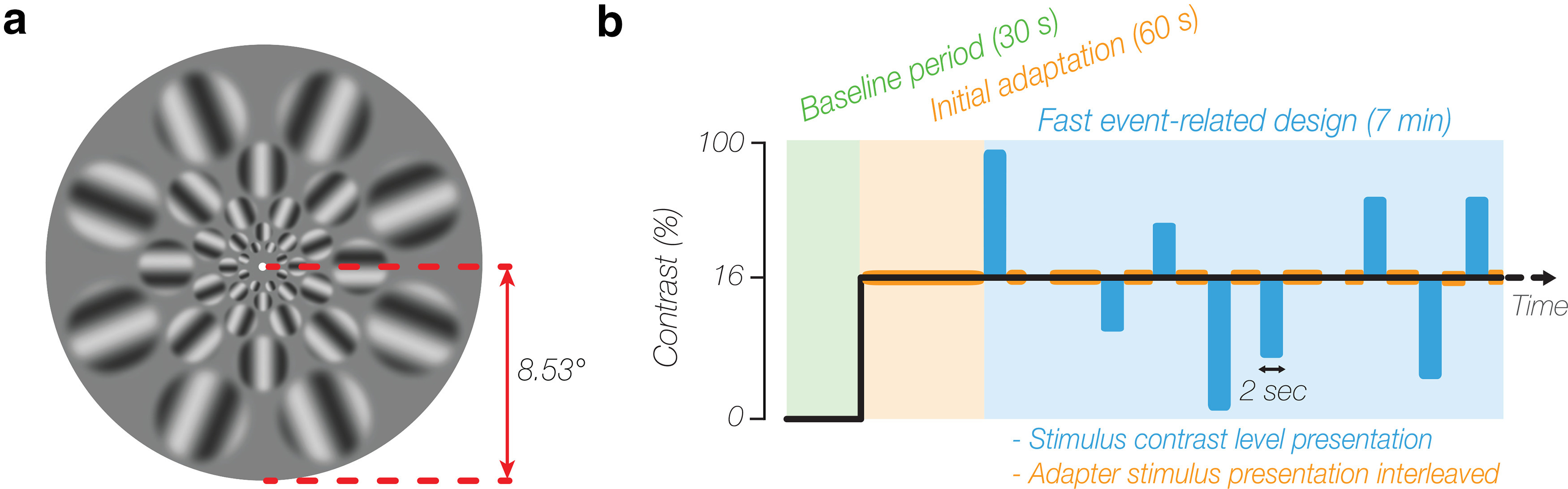
Measuring nonlinear contrast response functions using contrast adaptation and informed stimulus design. a, Cortically magnified stimulus. Experimental stimulus composed of gratings with radial orientations (relative to fixation) and cortically magnified spatial frequency (actual stimulus spatial frequency not depicted). b, Example adaptation and fast event-related fMRI run. Time line and organization of typical fMRI run for experiment 1, consisting primarily of fast event-related stimulus presentations (2 s duration) at multiple Michelson contrast levels, interleaved with the 16% contrast adapter stimulus to maintain adaptation throughout the entirety of each run. Each run began with a 30 s blank fixation baseline period (highlighted in green), followed by a 60 s sustained adaptation period (highlighted in orange) to promote contrast response homogeneity. For experiment 2, the initial adaptation period was not included, and interleaved contrast adapter stimulus presentation during the fast event-related period was replaced with blank fixation epochs.

Experimental design

The goals of each experiment were as follows: experiment 1, collect contrast responses following contrast adaptation; experiment 2, collect contrast responses without any explicit adaptation. All experimental data were collected over the course of two fMRI sessions. The adaptation condition was collected during session 1, and the adaptation-free (no adaptation) data were collected during session 2. A third additional fMRI session was dedicated to collecting anatomic images and data for population receptive field (pRF) mapping using standard techniques and stimuli (Dumoulin and Wandell, 2008; Kriegeskorte et al., 2008; Kay et al., 2013).

In all experiments, participants were presented with stimuli varying in contrast using a fast event-related design, making up the majority of each run (Fig. 1b). Stimuli were presented for a 2 s duration intermixed with a null period, consisting of either an adaptation top-up stimulus (16% contrast, adaptation condition) or a mean luminance background (0% contrast, adaptation-free condition). Null periods varied in duration between 4 and 17 s, with the overall experimental stimulus presentation timing generated using the Optseq2 optimization tool (Dale, 1999). The experimental presentation for experiment 1 was preceded by a 60 s initial adaptation block, during which participants were adapted to a 16% contrast stimulus with visual properties identical to the null period stimulus presented later in the event-related portion of the run. Previous studies have demonstrated that a 60 s adaptation period is sufficient to induce a stable adapted state of the human visual system (Blakemore and Campbell, 1969), and using a top-up adaptation stimulus during null periods mitigated any recovery from adaptation, serving to maintain the initial contrast adaptation state of the visual system throughout the experimental run (Foley and Boynton, 1993; Gardner et al., 2005). In the adaptation-free condition, participants were not presented with an initial adaptation block, mirroring the lack of any top-up adaptation stimulus during the fast event-related block null periods. For all experiments, the beginning of each experimental run began with a 30 s baseline period, during which participants viewed a uniform gray background (194.7 cd/m²). Participants completed three to five adaptation runs (8.5 min each, 510 TRs), and three to four no-adaptation runs (7.5 min each, 450 TRs), with six observations per stimulus contrast level collected per run.

For all fMRI experiments, participants fixated on a red dot at the center of the display (diameter, 0.11°) while being engaged in a rapid visual stream presentation (RSVP) task also located at fixation. The RSVP task consisted of a rapid sequential presentation of letters (35 point size), with target letters appearing with a 30% probability every 250 ms, after a minimum of 10 nontarget letters following the last target letter presentation. An MR-compatible response box was used to record behavioral responses to the RSVP task. Participants maintained high performance accuracy across all runs in both experiments (experiment 1, 97.4%; experiment 2, 98.1%).

MRI data acquisition

All neuroimaging data were collected on a research-dedicated Siemens Prisma 3T scanner using a 64-channel head coil. Whole-brain anatomic data were acquired using a T1-weighted multiecho MPRAGE 3D sequence (1mm³; FOV = 256 × 256 × 176 mm; flip angle (FA) = 7°; TR = 2530 ms; TE = 1.69 ms; van der Kouwe et al., 2008). All functional neuroimaging data (main experiments and pRF mapping) were acquired using a T2*-weighted in-plane simultaneous multislice imaging sequence (multiband factor, 3; Moeller et al., 2010; Xu et al., 2013), with the field of view oriented perpendicular to the calcarine sulcus (2 mm³; FOV = 60 × 112 × 172 mm; FA = 80°; TR = 1000 ms; TE = 35 ms).

Anatomical data analysis

Whole-brain T1-weighted anatomic data were analyzed using the standard recon-all pipeline provided by the FreeSurfer (Fischl, 2012) neuroimaging analysis package, generating cortical surface models, whole-brain segmentations, and cortical parcellations. Cortical surface models facilitated surface-based registration between structural and functional MRI volumes, allowing pRF analyses to be conveniently ported over to the native functional volume space.

Functional data analysis

EPI distortion correction was applied to all fMRI BOLD time series data using a reverse phase-encode method (Andersson et al., 2003) implemented in Functional MRI of the Brain Software Library (Smith et al., 2004). All fMRI preprocessing steps were completed with FreeSurfer Functional Analysis Stream (Fischl, 2012), including standard motion-correction procedures, Siemens slice timing correction, and boundary-based registration (Greve and Fischl, 2009) between functional and anatomic volumetric spaces. To facilitate voxelwise analyses, no volumetric spatial smoothing was performed (FWHM = 0 mm). Precise volumetric alignment of experimental condition data within each neuroimaging sessions was achieved using cross-run within-modality robust rigid registration (Reuter et al., 2010), with the middle time point of the first run from each session serving as the target volume, and the middle time point of each subsequent run from the session serving as the movable volume used for alignment. Before converting BOLD time series data to units of percent signal change, time points corresponding to the initial adaptation period (60 frames) were excluded when applicable. Data collected during the separate pRF mapping session were analyzed using the analyzePRF toolbox (Kay et al., 2013). Only voxels located within the cortical ribbon of the occipital lobe were designated for pRF modeling, which were identified using a visual area network label generated using an intrinsic functional connectivity atlas (Yeo et al., 2011).

For all fMRI experimental conditions, a univariate deconvolution analysis was conducted using a finite-impulse response (FIR) modeling approach (window size = 24 s, prestimulus delay = 4 s; Dale, 1999). This analysis provided a set of 24 β-weight parameters describing the time course of the BOLD response for each contrast level under investigation.

Voxel selection

The results from the pRF mapping were used to determine voxel selection within each region of interest (ROI). The pRF results were used to define the boundaries of all early visual areas (V1–V3), and identify candidate voxels within each visual area having eccentricity preferences bounded by stimulus dimensions (inner diameter, 0.7°; outer diameter, 9.1°). The pRF data for one participant were acquired with a slightly constrained visual angle, limiting reasonable eccentricity estimates, so the outer diameter limit for this participant was set to 8.9° during voxel selection. ROI labels were further constrained by excluding voxels with poor pRF modeling goodness of fit (r² < 20%), and unreasonably small population receptive field (RF) sizes (RF < 0.1°). Subsequently, for each participant within each experiment, the ROI-averaged deconvolution time course (FIR function) for the highest contrast condition (96%) was fit with a four-parameter Gaussian function for each early visual area (V1–V3). The mean and SD of the residual sum of squares when fitting the highest contrast condition with the Gaussian function was equivalent across adaptation (V1. 0.21 ± 0.08; V2, 0.15 ± 0.07; V3, 0.13 ± 0.08) and no adaptation conditions (V1, 0.22 ± 0.05; V2, 0.12 ± 0.06; V3, 0.10 ± 0.05). The best-fitting Gaussian function describing the ROI-averaged FIR function was then adjusted using linear regression (unbounded offset and amplitude scalar parameters) to best match the FIR function of each individual voxel contained within the ROI (96% contrast condition only). At the conclusion of this fitting procedure, the voxelwise goodness-of-fit (r² coefficient) was then used to create a metric ranging from 0 (worst fit) to 1 (best fit) for all voxels in each ROI. Voxels within each ROI were ranked according to their goodness-of-fit metric, with the top 40% selected for further analysis. Importantly, voxels with a high goodness-of-fit metric solely indicates that these particular voxels had a strong stimulus-evoked response to the highest contrast level, which was well described by a Gaussian function. This metric does not take into account the evoked responses at any other contrast level (<96%); thus, it serves as a voxel selection method that is agnostic to the overall qualitative shape of the contrast response function. Finally, any voxels with a maximal BOLD response exceeding 10% signal change were excluded in an effort to only include voxels with responses not attributable to draining vein hemodynamics, which are known to be significantly delayed in time relative to cortical gray matter (Lee et al., 1995) and are mainly expected to occur at the foveal confluence (Winawer et al., 2010). On average, this exclusion constituted <2% of all voxels across all participants. The total number of voxels (mean ± SEM across participants) that survived these selection criteria, after combining across left and right hemispheres, were as follows: experiment 1, V1, 209.6 ± 26.4; V2, 217.0 ± 20.6; V3, 207.8 ± 13.0; and experiment 2, V1, 265.8 ± 45.1; V2, 255.2 ± 35.8; V3, 223.3 ± 25.2.

Contrast response estimation

Final contrast response estimations were calculated by taking the average of the FIR modeling deconvolution β weights over a fixed and absolute window spanning 3 to 9 s poststimulus onset. These β weights were averaged together to produce a contrast response measurement for each of the nine contrast levels under investigation in each experiment. These contrast responses were used to create both ROI-specific and voxelwise response functions, which were then subjected to further analyses.

Model fitting and evaluation

To evaluate the degree to which contrast response functions are truly nonlinear in nature, the explanatory power of two different models were compared following a partially bounded least-squares fitting procedure in MATLAB (fmincon). The Naka–Rushton (NR) equation (Naka and Rushton, 1966) was selected as the candidate nonlinear function model as follows:

$$R\left(I\right)=R_{max}\cdot \frac{I^n}{I^n+C_{50}{}^n},$$

with R_max, C₅₀, and n corresponding to the maximal contrast response, semisaturation response, and overall rate of change (transducer), respectively. The upper bound of the maximal contrast response (R_max) was unconstrained, [0 Inf], whereas both the semisaturation response and transducer parameters were bounded respectively at [1 100] and [0 10]. Conversely, any linear tendencies of the contrast response functions were determined using a purely linear equation (2 unconstrained parameters; y-intercept and slope). Before any model fitting, all contrast responses were shifted by the mean response across the lowest three contrast levels (2.67, 4, and 5.33) at the ROI level to shift the response function baseline relative to zero. Following this baseline correction, the mean range and SD of BOLD activation was equivalent across adaptation (V1, 2.96 ± 0.51; V2, 2.17 ± 0.21; V3, 1.66 ± 0.39) and no adaptation (V1, 2.40 ± 0.54; V2, 1.61 ± 0.59; V3, 1.15 ± 0.43) experimental conditions and regions of interest. The contrast responses plotted in all result figures represent the baseline corrected BOLD response.

Statistical analyses

To identify the best-fitting model while also considering respective degrees of freedom, given the number of free parameters, the corrected Akaike information criterion (AIC_c) was computed for nonlinear and linear models (Banks and Joyner, 2017). A lower AIC_c score reflects a better dataset fit while penalizing for the number of free model parameters. The AIC_c difference between both candidate models was calculated (NR–linear), with negative values indicating the NR equation as the better fitting model and positive values indicating the linear equation as the better fitting model. We chose this approach because we are interested in comparing non-nested models using a metric derived from information theory, in which case statistical hypothesis testing (F tests) is not a viable approach (Motulsky and Christopoulos, 2004). Note that all reported AIC scores with model subscripts are also corrected AIC scores.

To assess the heteroscedasticity of model residuals, specifically whether the model prediction errors vary systematically (nonrandomly) across consecutive independent variable levels, a Durbin–Watson test statistic was calculated. Here, the statistic quantifies the prevalence of any lag 1 autocorrelation of residuals across successive contrast levels, with a groupwise Durbin–Watson d test statistic <1.5 signifying a positive autocorrelation. One-way between-subjects ANOVAs were performed to test for any differences in Naka–Rushton model parameter estimates across regions of interest and to test for any systematic differences in functional signal-to-noise ratio (SNR) measurements across regions of interest for both experiments 1 and 2. Significant effects were further investigated using pairwise t tests using Bonferroni correction. Significant monotonic trends between eccentricity preference, pRF size, and Naka–Rushton parameter estimates at the voxelwise level were evaluated using Spearman's correlations (r_s), with the correlations computed independently for each participant before being subjected to one-sample t tests using the Bonferroni correction to test whether the average correlation coefficient (r_s) across participants is significantly different from zero (no correlation).

Voxelwise functional SNR measurements were calculated based on the mean signal offset divided by the SD of the residuals following FIR model fitting. Specifically, the residuals reflect the difference between the estimated and actual BOLD time courses, and this method for estimating functional SNR is independent of any task signal and nuisance regressors.

Data availability

All fMRI datasets reported in this study, as well as all MATLAB code used for stimulus presentation and data analysis, are available at https://osf.io/8g6ap/.

Results

Sustained adaptation promotes nonlinear contrast responses

Does prolonged and sustained contrast adaptation promote nonlinear contrast response functions? We first measured the BOLD response evoked by nine different luminance contrast stimuli (Fig. 1a) following adaptation to a low-contrast level (Fig. 1b; see above, Materials and Methods). We then measured the BOLD response to the same contrast-varying stimuli again, but crucially this second experiment did not include sustained contrast adaptation. In both experiments, we performed a deconvolution analysis to obtain an average BOLD response for each contrast level under investigation. The ROI-averaged contrast responses collected following sustained contrast adaptation (experiment 1) are qualitatively different when compared with contrast responses collected in the absence of constrained contrast adaptation (experiment 2) across early visuocortical areas (example participant depicted in Fig. 2a).

Figure 2.

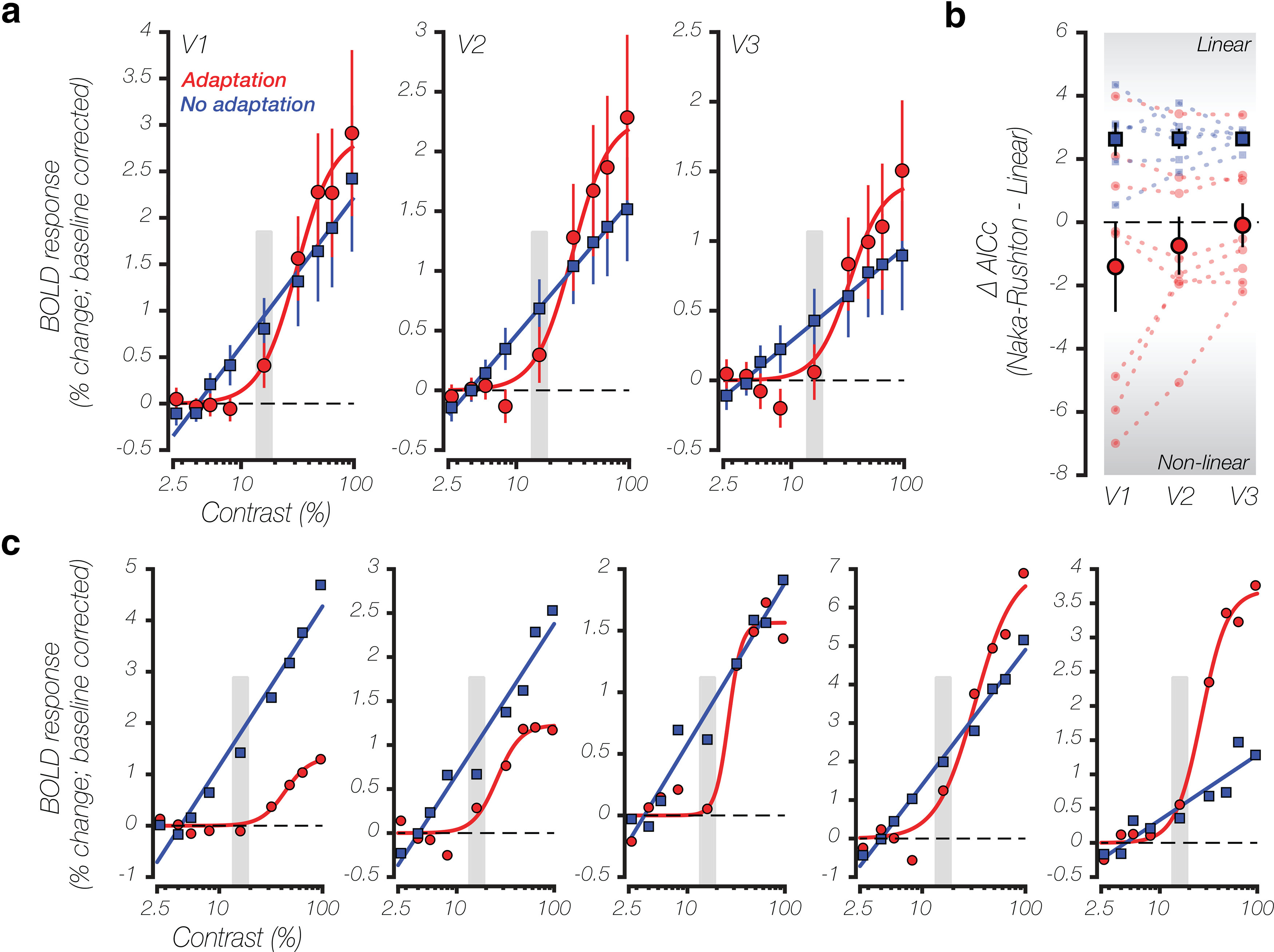
Sustained adaptation promotes nonlinear contrast responses within and across human visual cortex. a, Contrast response functions for example participant. ROI-averaged contrast response (mean BOLD percent signal change after baseline correction) of a representative participant plotted as a function of log-spaced Michelson contrast for each region of interest (V1–V3) for both adaptation (red circle) and no adaptation (blue square) conditions. Solid lines reflect the best-fit model (Naka–Rushton or linear function) for each respective experimental condition. Before fitting, all contrast responses were shifted by the mean response across the lowest three contrast levels at the ROI level to center the response function baseline around zero. Vertical dashed lines represent the 16% Michelson contrast level, corresponding to the adapter stimulus contrast level. Data are means ± half the SD across voxels. b, Model fit comparison. Individual and group-averaged voxelwise differences of the corrected AICc, comparing Naka–Rushton model fits to linear model fits for each region of interest and for both adaptation (red circle) and no adaptation (blue square) conditions. Negative values indicate the Naka–Rushton model is the most likely function to have generated the observed contrast responses. Small symbols with dashed lines denote individual participants (means ± SE across all voxels), and large symbols outlined in black denote group-averaged AICc difference scores (means ± SE across all participants). c, Voxelwise contrast response functions within area V1. Common patterns of contrast responses observed across experimental conditions at the voxelwise level within area V1 for the individual participant depicted in a. All voxels depicted survived cross-session registration and label transformation, and had <1° absolute difference in pRF eccentricity estimates across sessions. All data plotted using the same conventions as described in a.

To evaluate the degree to which sustained contrast adaptation promotes nonlinear population responses, we computed an ROI-averaged AIC_c metric that allowed for the comparison between model fits of a Naka–Rushton (nonlinear) and a linear model (Fig. 2b). Under contrast adaptation, AIC_c differences between the two models (AIC_Naka-Rushton and AIC_Linear), reported below as mean ± SE across participant, favored the Naka–Rushton model across all early visual areas (V1, −1.41 ± 1.43; V2, −0.74 ± 0.92; V3, −0.10 ± 0.69). In the absence of constrained contrast adaptation, AIC_c differences instead favored the linear model across all early visual areas (V1, 2.63 ± 0.52; V2, 2.64 ± 0.32; V3, 2.64 ± 0.11). Furthermore, the general juxtaposition of linear versus nonlinear response functions remains prevalent at the voxelwise level when comparing across adapt and no adapt conditions, respectively (Fig. 2c). Overall, this pattern of results demonstrates the profound impact that adaptation can have in shaping contrast response functions acquired with population-based measurements.

To better assess the heteroscedasticity of the model fitting across conditions, the model prediction errors (residuals) were plotted as a function of contrast level (Fig. 3) and compared using the Durbin-Watson autocorrelation test (DW_d), with a DW_d < 1.5 signifying a positive lag 1 autocorrelation. In the presence of adaptation, the linear function systematically failed to capture the variance across the midrange contrast levels, resulting in a positive autocorrelation across residuals for all ROIs (DW_d (V1) = 0.95, DW_d (V2) = 1.09, DW_d (V3) = 0.95), indicating that a linear function does not adequately describe the pattern of contrast responses measured in experiment 1. Conversely, the prediction error of the Naka–Rushton function lacks this systematic bias and does not display any autocorrelation across residuals for all ROIs (DW_d (V1) = 1.91, DW_d (V2) = 2.34, DW_d (V3) = 2.22), indicating that an inherently nonlinear function is necessary for describing the pattern of contrast responses measured in experiment 1. In the absence of constrained adaptation, however, both models displayed little to no systematic biases, with the linear model residuals having the weakest overall tendency toward a positive autocorrelation (linear model: DW_d (V1) = 1.91, DW_d (V2) = 1.58, DW_d (V3) = 1.72), and the Naka–Rushton model only having a slight bias in area V1 (Naka–Rushton model: DW_d (V1) = 1.25, DW_d (V2) = 1.72, DW_d (V3) = 1.52).

Figure 3.

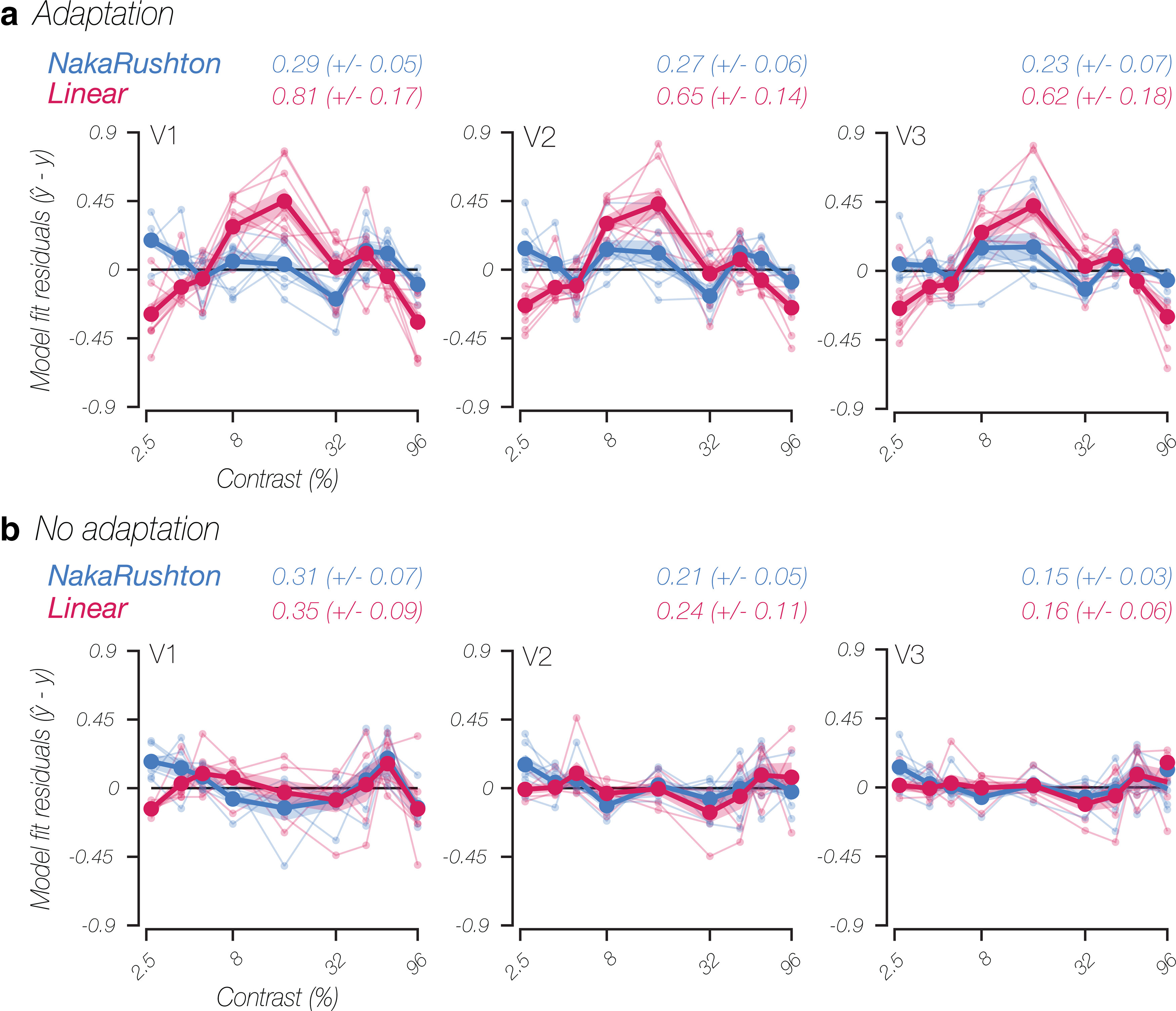
Systematic bias of model fit residuals; linear model inadequate with adaptation. a, Adaptation model fit heteroscedasticity. Individual and group-averaged model fit residuals plotted as a function of contrast level (log spaced) for both Naka–Rushton and linear model fits across regions of interest for data acquired following adaptation (experiment 1). Each plot depicts the prevalence of any systematic bias in model fits (heteroscedasticity). The mean sum of the squared error (± SE) across all participants is reported above each respective plot. b, No adaptation model fit heteroscedasticity. Model fit residuals for data acquired in the absence of constrained adaptation (experiment 2). All results plotted using the same conventions as described in a.

Voxelwise contrast response functions: Heterogeneity and trends within regions of interest

To ascertain the degree of heterogeneity within an ROI, contrast response functions were evaluated on a voxelwise basis. An NR equation was fit to voxelwise contrast responses only for experiment 1, where it was demonstrated that adaptation is required to capture the nonlinearity of the population response. The median estimated model parameters at the voxelwise level were computed for each participant, which were then averaged within each ROI across all participants, producing three parameters of interest (Fig. 4), reported below as mean ± SE across participants. The semisaturation constant estimate (C₅₀) remained relatively stable and low across ROIs (V1, 42.09 ± 5.75; V2, 40.02 ± 4.61; V3, 47.05 ± 5.30), reflecting the sustained low-contrast adaptation at 16% Michelson contrast, with no main effect of ROI (F_(2,21) = 0.47, p = 0.628). The transducer estimate (n) increased in steepness from striate to extrastriate ROIs (V1, 2.21 ± 0.20; V2, 3.12 ± 0.24; V3, 3.64 ± 0.42), confirmed by a main effect of ROI (F_(2,21) = 5.64, p = 0.011), with significant differences between V1 versus V2 (t₍₇₎ = −3.85, p_corrected = 0.019) and V1 versus V3 (t(7) = −4.18, p_corrected = 0.012) but not between V2 versus V3 (t₍₇₎ = −2.13, p_corrected = 0.212). Finally, the response saturation level (R_max) decreased in magnitude from striate to extrastriate ROIs (V1, 2.97 ± 0.36; V2, 1.89 ± 0.11; V3, 1.46 ± 0.13), confirmed by a main effect of ROI (F_(2,21) = 11.67, p < 0.001), with significant differences between V1 versus V2 (t₍₇₎ = 3.53, p_corrected = 0.029), V1 versus V3 (t₍₇₎ = 5.83, p_corrected = 0.002), and V2 versus V3 (t₍₇₎ = 4.81, p_corrected = 0.006). Finally, the significant differences observed across ROIs (V1–V3) are not simply because of monotonic changes in functional SNR (see above, Materials and Methods) across the visual hierarchy (F_(2,21) = 0.25, p = 0.777). In general, the different patterns of transducer and response saturation estimates across the visuocortical hierarchy reflect hallmarks of nonlinear contrast response functions previously reported in the literature (Levitt et al., 1994; Avidan et al., 2002), whereas the consistent semisaturation estimates across early visual areas seen here are analogous to those of previous reports (Albrecht and Hamilton, 1982; Sclar et al., 1990).

Figure 4.

Voxelwise Naka–Rushton model parameter estimates (adaptation condition). Individual and group-averaged voxelwise Naka–Rushton function parameter estimates describing contrast responses following adaptation for each region of interest (V1–V3). Colored circles identify the median voxelwise parameter estimate for each individual participant, whereas gray circles denote the group-averaged parameter estimates (means ± SE). Note that semisaturation estimates are plotted on log scale, with the dashed line corresponding to 16% Michelson contrast. Asterisks denote significant t test results (*p_corrected < 0.05, **p_corrected < 0.01).

Although the semisaturation constant estimates at the participant level did not vary across the visual hierarchy (Fig. 4), several interesting trends were found at the voxelwise level. Semisaturation constant estimates displayed a significant monotonic Spearman's correlation with the distance of the preferred visual field location from fixation (eccentricity), being estimated by the pRF method, within each early visual area (V1–V3; V1, r_s = 0.35 ± 0.06, t₍₇₎ = 5.82, p_corrected < 0.001; V2, r_s = 0.41 ± 0.06, t(7) = 7.03, p_corrected < 0.001; V3, r_s = 0.28 ± 0.06, t₍₇₎ = 4.94, p_corrected = 0.005). Voxelwise semisaturation constant estimates were also found to be positively correlated with response saturation level (V1, r_s = 0.36 ± 0.05, t₍₇₎ = 7.72, p_corrected < 0.001; V2, r_s = 0.20 ± 0.05, t₍₇₎ = 3.95, p_corrected = 0.017; V3, r_s = 0.34 ± 0.03, t₍₇₎ = 9.96, p_corrected < 0.001), and negatively correlated with transducer steepness (V1, r_s = −0.49 ± 0.04, t₍₇₎ = −11.85, p_corrected < 0.001; V2, r_s = −0.32 ± 0.05, t₍₇₎ = −6.69, p_corrected < 0.001; V3, r_s = −0.26 ± 0.05, t₍₇₎ = −5.05, p_corrected = 0.005) consistently for all early visuocortical areas (Fig. 5a,b). However, the eccentricity bias did not generalize in the same consistent manner to any other voxelwise Naka–Rushton parameter estimates, with response saturation level displaying only a negative eccentricity bias in area V2 (V1, r_s = −0.02 ± 0.05, t₍₇₎ = −0.37, p_corrected = 1; V2, r_s = −0.15 ± 0.04, t₍₇₎ = −3.71, p_corrected = 0.023; V3, r_s = −0.05 ± 0.04, t₍₇₎ = −1.45, p_corrected = 0.573) and transducer steepness only displaying a positive eccentricity bias in area V3 (V1, r_s = 0.004 ± 0.06, t₍₇₎ = 0.06, p_corrected = 1; V2, r_s = 0.12 ± 0.04, t₍₇₎ = 3.00, p_corrected = 0.06; V3, r_s = 0.16 ± 0.05, t₍₇₎ = 3.23, p_corrected = 0.043), although response saturation level and transducer steepness estimates did display a strong negative correlation with each other across all early visuocortical areas (V1, r_s = −0.49 ± 0.04, t₍₇₎ = −12.08, p_corrected < 0.001; V2, r_s = −0.47 ± 0.06, t₍₇₎ = −8.51, p_corrected < 0.001; V3, r_s = −0.47 ± 0.06, t₍₇₎ = −8.08, p_corrected < 0.001). On average across participants, 15.5% of voxels within each ROI were found to have bounded semisaturation constant estimates at or near 100% contrast. Despite bounded fitting, these voxels were not excluded because they had reliable pRF estimates and survived the voxel selection procedure, and the exclusion of these particular voxels does not alter the general pattern of results. Specifically, excluding these bounded voxels (C₅₀ > = 99) did not significantly alter the AICc difference scores for each ROI within the contrast adaptation condition (V1, −1.40 ± 1.47, t₍₇₎ = 0.05, p_corrected = 1; V2, −0.86 ± 0.96, t₍₇₎ = −1.89, p_corrected = 0.302; V3, −0.15 ± 0.73, t₍₇₎ = −0.81, p_corrected = 1).

Figure 5.

Voxelwise contrast response functions, heterogeneity, and trends within region of interest. a, Voxelwise eccentricity bias. Log–log scatter plots depicting voxelwise semisaturation parameter estimates covarying with visual field eccentricity preference, which corresponds to the pRF estimate of the response field center (in degrees of visual angle radiating out from fixation) for each respective voxel included in each ROI analysis. Data point color scale depicts the corresponding response saturation (R_max) parameter estimate for each particular voxel being plotted. Black circles denote binned group-averaged median parameter estimates. Error bars were asymmetric and uninformative when plotted on a log scale and have been omitted. Black dashed lines correspond to 16% Michelson contrast. b, All data plotted using the same conventions as described in a, with the exception that the data point color scale depicts the corresponding transducer (n) parameter estimate for each particular voxel being plotted. c, Groupwise eccentricity bias. Mean eccentricity-based contrast responses (BOLD percent signal change after baseline correction) of each participant plotted as a function of log-spaced Michelson contrast for each region of interest (V1–V3). Each respective solid-colored line reflects the best-fit Naka–Rushton function to the group-averaged contrast responses within each mutually exclusive eccentricity range defined by the colored brackets in a and b. All individual participant contrast responses within each eccentricity range are plotted in low opacity. Triangle symbols denote the value of the semisaturation parameter estimate for each respective eccentricity range.

When averaging the voxelwise contrast responses coarsely binned by eccentricity, it becomes apparent that the population-based CRFs are centered at progressively higher contrast levels as the preferred visual field location shifts farther away from fixation (Fig. 5c). It has been well established that RF size and eccentricity preference strongly covary with one another in early visuocortical areas (Dow et al., 1981; Smith et al., 2001; Harvey and Dumoulin, 2011). If the interaction between semisaturation constant estimates and eccentricity reported above is not a spurious finding, semisaturation constant estimates should also covary with population RF size within each ROI, which was found to be the case (V1, r_s = 0.20 ± 0.04, t₍₇₎ = 5.43, p_corrected < 0.001; V2, r_s = 0.29 ± 0.05, t₍₇₎ = 6.34, p_corrected < 0.001; V3, r_s = 0.23 ± 0.05, t₍₇₎ = 5.20, p_corrected = 0.004). However, although both sets of correlations are significant, these findings indicate that additional factors in addition to eccentricity and RF size contribute to the variation of semisaturation constant estimates we observed within human visual cortex. No consistent RF size biases were found for response saturation level (V1, r_s = 0.09 ± 0.05, t₍₇₎ = 1.85, p_corrected = 0.321; V2, r_s = −0.01 ± 0.04, t₍₇₎ = −0.32, p_corrected = 1; V3, r_s = −0.04 ± 0.04, t₍₇₎ −1.05, p_corrected = 0.986) and transducer steepness (V1, r_s = −0.03 ± 0.05, t₍₇₎ = −0.68, p_corrected = 1; V2, r_s = 0.06 ± 0.05, t₍₇₎ = 1.35, p_corrected = 0.662; V3, r_s = 0.14 ± 0.04, t₍₇₎ = 3.24, p_corrected = 0.043), congruent with the pattern of eccentricity bias results reported above.

Discussion

Although nonlinearities have often been considered a trademark property of neural responses, functional neuroimaging measures of response profiles have tended to appear puzzlingly linear. In this study, we find evidence to suggest that sustained adaptation plays a key role in promoting nonlinear population-based contrast response functions in the human visual cortex. The Naka–Rushton parameter estimates we obtained are coincident with previous reports of contrast response variability across the visual hierarchy. Crucially, a linear function proved to be inadequate in capturing the pattern of population-based contrast responses, highlighted by a systematic fitting bias across contrast levels. In the absence of constrained contrast adaptation, a qualitatively different pattern of contrast responses was observed, best captured by a linear model, consistent with the bulk of previous population-based contrast responses measured in humans (Tootell et al., 1995, 1998; Boynton et al., 1996, 1999; Buracas et al., 2005; Buracas and Boynton, 2007; Murray, 2008; Pestilli et al., 2011; Itthipuripat et al., 2019).

How might constrained adaptation have such a profound effect on contrast responsivity in early visual cortex? Adaptation is a naturally occurring everyday phenomenon, constantly operating to reflect statistical regularities in our environment and helping to maintain high sensitivity within a particular stimulus range (Clifford et al., 2007; Kohn, 2007). In the visual modality, contrast adaptation has been shown to alter perception in systematic ways, improving sensitivity within the adapted range (Foley and Boynton, 1993). At the neural level, contrast adaptation serves to recenter the response profiles of individual units toward the average contrast level of the visual environment (Ohzawa et al., 1985; Sclar et al., 1989; Carandini and Ferster, 1997) within a relatively short period of time (30–60 s; Blakemore and Campbell, 1969; Movshon and Lennie, 1979; Albrecht et al., 1984; Gardner et al., 2005). The population response captured by the fMRI BOLD signal encompasses quite a large number and variety of neurons with a broad heterogeneity of nonlinear response profiles known to be present at this submillimeter level (Albrecht and Hamilton, 1982; Sclar et al., 1990). Recalibration during adaptation may serve to reduce this neural response heterogeneity within local neural populations insomuch as to preserve the nonlinear response properties even after pooling across the population. Indeed, it has been demonstrated that in the absence of any explicit adaptation, averaging over a heterogeneous neural population can aggregate a multitude of nonlinear neural contrast response functions into a qualitatively different population response within both experimental (Albrecht and Hamilton, 1982) and modeling (Hara et al., 2014) contexts. Therefore, by bringing the sensitivity of a heterogenous array of nonlinear response functions into closer alignment, subsequent population response measurements, such as fMRI, may then summarize a more homogenous population response, capturing a nonlinear representation of the underlying neural units (Fig. 6).

Figure 6.

Contrast gain changes reducing neural response heterogeneity to produce a nonlinear population contrast response function. Conceptual illustration demonstrating how sustained contrast adaptation potentially induces nonlinear population contrast response functions by bringing individual neural units within the population into closer alignment via contrast gain changes (e.g., horizontal shifts).

As adaptation is an ongoing process, it is worthwhile to consider what recalibration was taking place in the absence of any constrained contrast adaptation. One consideration is that by removing the initial adaptation period to the 16% contrast stimulus and presenting a mean gray blank fixation (0% contrast) during interleaved periods, the average contrast level encountered throughout a single functional run was much lower than 16%. Having adapted to a lower contrast level under unconstrained adaptation settings, one would expect response functions to have shifted even farther to the left relative to the response functions we observed following adaptation to 16% contrast. However, this was not what we observed, instead finding nonsaturating response functions largely centered at higher contrast levels, suggesting a qualitatively different contrast responsivity change is occurring after prolonged viewing consisting mainly of uniform and diffusely illuminated stimuli (0% contrast). Additionally, we observed a general reduction in responsivity at high contrast levels in the absence of adaptation, which suggests processes other than contrast sensitivity were being altered during adaptation. Previous modeling work has linked intracortical inhibition to changes in response saturation (Todorov et al., 1997), with lower R_max estimates expected when adapting to progressively higher contrast levels, which has previously been shown to be the case in cat striate cortex (Albrecht et al., 1984). However, if the unconstrained adaptation condition is considered as having induced adaptation to a contrast level lower than 16%, given the average stimulus contrast level encountered throughout any given run, then our results demonstrate the opposite relationship. This contradiction suggests that it may be misleading to classify a uniform and diffusely illuminated stimulus as being 0% contrast and that this extreme contrast level should not be treated the same as nonzero contrast level stimuli. Suffice it to say, the effects of contrast adaptation may well extend beyond straightforward contrast sensitivity changes, with further experimental evidence needed to clarify exactly how, and under what conditions, various gain control processes interact with one another.

Undoubtedly, another important contribution to the contrast response nonlinearities we report is the use of an event-related experimental design rather than a blocked design. The latter design type has considerable downsampling and hysteresis caveats that are detrimental to capturing nonlinear contrast responses. When taking the block-averaged BOLD response to represent a particular contrast response, the average of the entire decaying BOLD time series within the block is not necessarily analogous to the evoked response for any particular stimulus condition when the contrast response nuances are most prevalent as the initial evoked response at the beginning of each block. Improvements in modeling BOLD response variability measured with blocked designs has been reported when including a decaying exponential function for neural response during each stimulus block (Boynton et al., 1996), or when using a sinusoidal period instead of a square wave to model ON/OFF stimulus periods (Boynton et al., 1999; Buracas et al., 2005). Additionally, in some instances the block-averaged response to a low-contrast stimulus may be overwhelmingly negative relative to initial baseline if that particular block is preceded by a stimulus block during which adaptation to a significantly higher contrast level has occurred. Stimulus differences between our study and other event-related fMRI studies highlight other potential contributions to the overall potency and breadth of activity we see within early visual areas. Crucial stimulus properties include stimulus position (peripheral vs centered at fixation), overall size, spatial frequency (fixed vs cortically magnified), and local orientation relative to the visual meridians and fixation (radial orientation bias; Sasaki et al., 2006; Mannion et al., 2010; Freeman et al., 2011).

These aforementioned methodological concerns are not only relegated to fMRI-based population measurements of responses; indeed, they generalize to many measures, and in particular any population-based measure that succumbs to these pitfalls can misleadingly produce linear results. Optical imaging spectroscopy is an alternate population-based measurement of brain function operating at higher temporal resolutions while also being based on changes in hemodynamics and blood oxygenation levels (Malonek and Grinvald, 1996). Contrast response function obtained in animals using optical imaging have resulted in reports of largely linear response profiles in areas V1 and V2 for both cats (Carandini and Sengpiel, 2004; Zhan et al., 2005) and nonhuman primates (Lu and Roe, 2007). It remains to be clearly seen whether contrast adaptation can also alter the contrast response function measured in optical imaging studies, although some insight is provided by studies examining orientation tuning under different adaptation states across very few contrast levels (Dragoi et al., 2000; Sengpiel and Bonhoeffer, 2002).

Electroencephalography (EEG) offers a qualitatively different measure of neural population activity, based largely on electrical activity generated from postsynaptic potentials located within cortical layers oriented parallel to electrodes on the scalp (da Silva, 2013). Despite having a coarser spatial resolution, nonlinear contrast responses are relatively common in the literature (Reynolds et al., 2000; Di Russo et al., 2001; Itthipuripat et al., 2019). However, it is likely that these EEG results reflect a biased, narrower sample of population activity, driven by a handful of focally potent signals because of intraregional cortical folding and stimulus feature preferences, and dependent on particular event-related potential components, frequency band (Kappenman and Luck, 2016; Hermes et al., 2017), or the source-localization technique used (Grech et al., 2008). Finally, studies are beginning to reveal that the neurovascular coupling between BOLD response and neural activation is a dynamic relationship that can be systematically altered across stimulus intensity (i.e., contrast; Liang et al., 2013), stimulus duration (Boynton et al., 1996; Thompson et al., 2014), and stimulus flicker frequency (Lin et al., 2008). Although these changes in neurovascular coupling may have been at play in the given study, they would have been consistent across both experimental conditions and cannot account for the impact of adaptation on contrast response nonlinearities.

Achieving an accurate portrayal of the various ongoing nonlinear gain control operations (i.e., arousal and attention) may ultimately require leveraging what we already know about other properties of the human CNS. When measuring population-based activity, presenting weak or nonpreferred stimuli may not be sufficient for a complete response profile to emerge. Going forward, careful consideration of stimulus properties and incorporating sustained adaptation into experimental designs will allow for more robust computational modeling by using data from both animal and human findings, as well as being able to capture functional variability across multiple spatial scales of measurement. By acquiring a comprehensive understanding of how the human brain adapts and responds to the environment, we can better discern the local and global neural circuitry supporting human sensation and perception.

References

- Albrecht DG, Hamilton DB (1982) Striate cortex of monkey and cat: contrast response function. J Neurophysiol 48:217–237. 10.1152/jn.1982.48.1.217 [DOI] [PubMed] [Google Scholar]
- Albrecht DG, Farrar SB, Hamilton DB (1984) Spatial contrast adaptation characteristics of neurones recorded in the cat's visual cortex. J Physiol 347:713–739. 10.1113/jphysiol.1984.sp015092 [DOI] [PMC free article] [PubMed] [Google Scholar]
- Andersson JLR, Skare S, Ashburner J (2003) How to correct susceptibility distortions in spin-echo echo-planar images: application to diffusion tensor imaging. Neuroimage 20:870–888. 10.1016/S1053-8119(03)00336-7 [DOI] [PubMed] [Google Scholar]
- Avidan G, Harel M, Hendler T, Ben-Bashat D, Zohary E, Malach R (2002) Contrast sensitivity in human visual areas and its relationship to object recognition. J Neurophysiol 87:3102–3116. 10.1152/jn.2002.87.6.3102 [DOI] [PubMed] [Google Scholar]
- Banks HT, Joyner ML (2017) AIC under the framework of least squares estimation. App Math Lett 74:33–45. 10.1016/j.aml.2017.05.005 [DOI] [Google Scholar]
- Blakemore C, Campbell FW (1969) On the existence of neurones in the human visual system selectively sensitive to the orientation and size of retinal images. J Physiol 203:237–260. 10.1113/jphysiol.1969.sp008862 [DOI] [PMC free article] [PubMed] [Google Scholar]
- Bonds AB (1991) Temporal dynamics of contrast gain in single cells of the cat striate cortex. Vis Neurosci 6:239–255. 10.1017/s0952523800006258 [DOI] [PubMed] [Google Scholar]
- Boynton GM, Engel SA, Glover GH, Heeger DJ (1996) Linear systems analysis of functional magnetic resonance imaging in human V1. J Neurosci 16:4207–4221. 10.1523/JNEUROSCI.16-13-04207.1996 [DOI] [PMC free article] [PubMed] [Google Scholar]
- Boynton GM, Demb JB, Glover GH, Heeger DJ (1999) Neuronal basis of contrast discrimination. Vision Res 39:257–269. 10.1016/s0042-6989(98)00113-8 [DOI] [PubMed] [Google Scholar]
- Brainard DH (1997) The Psychophysics Toolbox. Spat Vis 10:433–436. [PubMed] [Google Scholar]
- Buracas GT, Boynton GM (2007) The effect of spatial attention on contrast response functions in human visual cortex. J Neurosci 27:93–97. 10.1523/JNEUROSCI.3162-06.2007 [DOI] [PMC free article] [PubMed] [Google Scholar]
- Buracas GT, Fine I, Boynton GM (2005) The relationship between task performance and functional magnetic resonance imaging response. J Neurosci 25:3023–3031. 10.1523/JNEUROSCI.4476-04.2005 [DOI] [PMC free article] [PubMed] [Google Scholar]
- Carandini M, Heeger DJ (1994) Summation and division by neurons in primate visual cortex. Science 264:1333–1336. 10.1126/science.8191289 [DOI] [PubMed] [Google Scholar]
- Carandini M, Ferster D (1997) A tonic hyperpolarization underlying contrast adaptation in cat visual cortex. Science 276:949–952. 10.1126/science.276.5314.949 [DOI] [PubMed] [Google Scholar]
- Carandini M, Sengpiel F (2004) Contrast invariance of functional maps in cat primary visual cortex. J Vis 4(3):1 1–14. 10.1167/4.3.1 [DOI] [PubMed] [Google Scholar]
- Carandini M, Heeger DJ, Movshon JA (1997) Linearity and normalization of simple cells of the macaque primary visual. J Neurosci 17:8621–8644. 10.1523/JNEUROSCI.17-21-08621.1997 [DOI] [PMC free article] [PubMed] [Google Scholar]
- Carandini M, Heeger DJ, Movshon JA (1999) Linearity and gain control in V1 simple cells. In: Models of cortical circuits, cerebral cortex, pp 401–443. Boston, MA:Springer. [Google Scholar]
- Clifford CWG, Webster MA, Stanley GB, Stocker AA, Kohn A, Sharpee TO, Schwartz O (2007) Visual adaptation: neural, psychological and computational aspects. Vision Res 47:3125–3131. 10.1016/j.visres.2007.08.023 [DOI] [PubMed] [Google Scholar]
- da Silva FL (2013) EEG and MEG: relevance to neuroscience. Neuron 80:1112–1128. [DOI] [PubMed] [Google Scholar]
- Dale AM (1999) Optimal experimental design for event-related fMRI. Hum Brain Mapp 8:109–114. [DOI] [PMC free article] [PubMed] [Google Scholar]
- Dean AF (1981) The relationship between response amplitude and contrast for cat striate cortical neurones. J Physiol 318:413–427. 10.1113/jphysiol.1981.sp013875 [DOI] [PMC free article] [PubMed] [Google Scholar]
- Di Russo F, Spinelli D, Morrone MC (2001) Automatic gain control contrast mechanisms are modulated by attention in humans: evidence from visual evoked potentials. Vision Res 41:2435–2447. 10.1016/s0042-6989(01)00134-1 [DOI] [PubMed] [Google Scholar]
- DiCarlo JJ, Zoccolan D, Rust NC (2012) How does the brain solve visual object recognition? Neuron 73:415–434. 10.1016/j.neuron.2012.01.010 [DOI] [PMC free article] [PubMed] [Google Scholar]
- Dow BM, Snyder AZ, Vautin RG, Bauer R (1981) Magnification factor and receptive field size in foveal striate cortex of the monkey. Exp Brain Res 44:213–228. 10.1007/BF00237343 [DOI] [PubMed] [Google Scholar]
- Dragoi V, Sharma J, Sur M (2000) Adaptation-induced plasticity of orientation tuning in adult visual cortex. Neuron 28:287–298. 10.1016/s0896-6273(00)00103-3 [DOI] [PubMed] [Google Scholar]
- Dumoulin SO, Wandell BA (2008) Population receptive field estimates in human visual cortex. Neuroimage 39:647–660. 10.1016/j.neuroimage.2007.09.034 [DOI] [PMC free article] [PubMed] [Google Scholar]
- Fischl B (2012) FreeSurfer. Neuroimage 62:774–781. 10.1016/j.neuroimage.2012.01.021 [DOI] [PMC free article] [PubMed] [Google Scholar]
- Foley JM, Boynton GM (1993) Forward pattern masking and adaptation: effects of duration, interstimulus interval, contrast, and spatial and temporal frequency. Vision Res 33:959–980. 10.1016/0042-6989(93)90079-C [DOI] [PubMed] [Google Scholar]
- Freeman J, Brouwer GJ, Heeger DJ, Merriam EP (2011) Orientation decoding depends on maps, not columns. J Neurosci 31:4792–4804. 10.1523/JNEUROSCI.5160-10.2011 [DOI] [PMC free article] [PubMed] [Google Scholar]
- Gardner JL, Sun P, Waggoner RA, Ueno K, Tanaka K, Cheng K (2005) Contrast adaptation and representation in human early visual cortex. Neuron 47:607–620. 10.1016/j.neuron.2005.07.016 [DOI] [PMC free article] [PubMed] [Google Scholar]
- Grech R, Cassar T, Muscat J, Camilleri KP, Fabri SG, Zervakis M, Xanthopoulos P, Sakkalis V, Vanrumste B (2008) Review on solving the inverse problem in EEG source analysis. J Neuroeng Rehabil 5:25–33. 10.1186/1743-0003-5-25 [DOI] [PMC free article] [PubMed] [Google Scholar]
- Greenlee MW, Georgeson MA, Magnussen S, Harris JP (1991) The time course of adaptation to spatial contrast. Vision Res 31:223–236. 10.1016/0042-6989(91)90113-j [DOI] [PubMed] [Google Scholar]
- Greve DN, Fischl B (2009) Accurate and robust brain image alignment using boundary-based registration. Neuroimage 48:63–72. 10.1016/j.neuroimage.2009.06.060 [DOI] [PMC free article] [PubMed] [Google Scholar]
- Hara Y, Gardner JL (2014) Encoding of graded changes in spatial specificity of prior cues in human visual cortex. J Neurophysiol 112:2834–2849. 10.1152/jn.00729.2013 [DOI] [PubMed] [Google Scholar]
- Hara Y, Pestilli F, Gardner JL (2014) Differing effects of attention in single-units and populations are well predicted by heterogeneous tuning and the normalization model of attention. Front Comput Neurosci 8:12. [DOI] [PMC free article] [PubMed] [Google Scholar]
- Harvey BM, Dumoulin SO (2011) The relationship between cortical magnification factor and population receptive field size in human visual cortex: constancies in cortical architecture. J Neurosci 31:13604–13612. 10.1523/JNEUROSCI.2572-11.2011 [DOI] [PMC free article] [PubMed] [Google Scholar]
- Heeger DJ (1992) Normalization of cell responses in cat striate cortex. Vis Neurosci 9:181–197. 10.1017/s0952523800009640 [DOI] [PubMed] [Google Scholar]
- Hermes D, Nguyen M, Winawer J (2017) Neuronal synchrony and the relation between the blood-oxygen-level dependent response and the local field potential. PLoS Biol 15:e2001461. 10.1371/journal.pbio.2001461 [DOI] [PMC free article] [PubMed] [Google Scholar]
- Ho WA, Berkley MA (1988) Evoked potential estimates of the time course of adaptation and recovery to counterphase gratings. Vision Res 28:1287–1296. 10.1016/0042-6989(88)90059-4 [DOI] [PubMed] [Google Scholar]
- Itthipuripat S, Sprague TC, Serences JT (2019) Functional MRI and EEG index complementary attentional modulations. J Neurosci 39:6162–6179. 10.1523/JNEUROSCI.2519-18.2019 [DOI] [PMC free article] [PubMed] [Google Scholar]
- Kappenman ES, Luck SJ (2016) Best practices for event-related potential research in clinical populations. Biol Psychiatry Cogn Neurosci Neuroimaging 1:110–115. 10.1016/j.bpsc.2015.11.007 [DOI] [PMC free article] [PubMed] [Google Scholar]
- Kay KN, Winawer J, Mezer A, Wandell BA (2013) Compressive spatial summation in human visual cortex. J Neurophysiol 110:481–494. 10.1152/jn.00105.2013 [DOI] [PMC free article] [PubMed] [Google Scholar]
- Kohn A (2007) Visual adaptation: physiology, mechanisms, and functional benefits. J Neurophysiol 97:3155–3164. 10.1152/jn.00086.2007 [DOI] [PubMed] [Google Scholar]
- Kriegeskorte N, Mur M, Ruff DA, Kiani R, Bodurka J, Esteky H, Tanaka K, Bandettini PA (2008) Matching categorical object representations in inferior temporal cortex of man and monkey. Neuron 60:1126–1141. 10.1016/j.neuron.2008.10.043 [DOI] [PMC free article] [PubMed] [Google Scholar]
- Lee AT, Glover GH, Meyer CH (1995) Discrimination of large venous vessels in time-course spiral blood-oxygen-level-dependent magnetic-resonance functional neuroimaging. Magn Reson Med 33:745–754. 10.1002/mrm.1910330602 [DOI] [PubMed] [Google Scholar]
- Levitt JB, Kiper DC, Movshon JA (1994) Receptive fields and functional architecture of macaque V2. J. Neurophysiol 71:2517–2542. [DOI] [PubMed] [Google Scholar]
- Li X, Lu Z-L, Tjan BS, Dosher BA, Chu W (2008) Blood oxygenation level-dependent contrast response functions identify mechanisms of covert attention in early visual areas. Proc Natl Acad Sci U S A 105:6202–6207. 10.1073/pnas.0801390105 [DOI] [PMC free article] [PubMed] [Google Scholar]
- Liang CL, Ances BM, Perthen JE, Moradi F, Liau J, Buracas GT, Hopkins SR, Buxton RB (2013) Luminance contrast of a visual stimulus modulates the BOLD response more than the cerebral blood flow response in the human brain. Neuroimage 64:104–111. 10.1016/j.neuroimage.2012.08.077 [DOI] [PMC free article] [PubMed] [Google Scholar]
- Lin A-L, Fox PT, Yang Y, Lu H, Tan L-H, Gao J-H (2008) Evaluation of MRI models in the measurement of CMRO2 and its relationship with CBF. Magn Reson Med 60:380–389. 10.1002/mrm.21655 [DOI] [PMC free article] [PubMed] [Google Scholar]
- Lu HD, Roe AW (2007) Optical imaging of contrast response in macaque monkey V1 and V2. Cereb Cortex 17:2675–2695. 10.1093/cercor/bhl177 [DOI] [PubMed] [Google Scholar]
- Malonek D, Grinvald A (1996) Interactions between electrical activity and cortical microcirculation revealed by imaging spectroscopy: implications for functional brain mapping. Science 272:551–554. 10.1126/science.272.5261.551 [DOI] [PubMed] [Google Scholar]
- Mannion DJ, McDonald JS, Clifford CWG (2010) Orientation anisotropies in human visual cortex. J Neurophysiol 103:3465–3471. 10.1152/jn.00190.2010 [DOI] [PubMed] [Google Scholar]
- Marquardt I, Schneider M, Gulban OF, Ivanov D, Uludağ K (2018) Cortical depth profiles of luminance contrast responses in human V1 and V2 using 7 T fMRI. Hum Brain Mapp 39:2812–2827. 10.1002/hbm.24042 [DOI] [PMC free article] [PubMed] [Google Scholar]
- Moeller S, Yacoub E, Olman CA, Auerbach E, Strupp J, Harel N, Uğurbil K (2010) Multiband multislice GE-EPI at 7 tesla, with 16-fold acceleration using partial parallel imaging with application to high spatial and temporal whole-brain fMRI. Magn Reson Med 63:1144–1153. 10.1002/mrm.22361 [DOI] [PMC free article] [PubMed] [Google Scholar]
- Motulsky H, Christopoulos A (2004) Fitting models to biological data using linear and nonlinear regression: a practical guide to curve fitting. New York: Oxford University Press. [Google Scholar]
- Movshon JA, Lennie P (1979) Pattern-selective adaptation in visual cortical neurones. Nature 278:850–852. 10.1038/278850a0 [DOI] [PubMed] [Google Scholar]
- Murray SO (2008) The effects of spatial attention in early human visual cortex are stimulus independent. J Vis. 8(10):2. 10.1167/8.10.2 [DOI] [PubMed] [Google Scholar]
- Naka KI, Rushton WA (1966) S-potentials from luminosity units in the retina of fish (Cyprinidae). J Physiol 185:587–599. 10.1113/jphysiol.1966.sp008003 [DOI] [PMC free article] [PubMed] [Google Scholar]
- Ohzawa I, Sclar G, Freeman RD (1985) Contrast gain control in the cat's visual system. J Neurophysiol 54:651–667. 10.1152/jn.1985.54.3.651 [DOI] [PubMed] [Google Scholar]
- Pestilli F, Carrasco M, Heeger DJ, Gardner JL (2011) Attentional enhancement via selection and pooling of early sensory responses in human visual cortex. Neuron 72:832–846. 10.1016/j.neuron.2011.09.025 [DOI] [PMC free article] [PubMed] [Google Scholar]
- Polimeni JR, Balasubramanian M, Schwartz EL (2006) Multi-area visuotopic map complexes in macaque striate and extra-striate cortex. Vision Res 46:3336–3359. 10.1016/j.visres.2006.03.006 [DOI] [PMC free article] [PubMed] [Google Scholar]
- Priebe NJ, Ferster D (2012) Mechanisms of neuronal computation in mammalian visual cortex. Neuron 75:194–208. 10.1016/j.neuron.2012.06.011 [DOI] [PMC free article] [PubMed] [Google Scholar]
- Reuter M, Rosas HD, Fischl B (2010) Highly accurate inverse consistent registration: a robust approach. Neuroimage 53:1181–1196. 10.1016/j.neuroimage.2010.07.020 [DOI] [PMC free article] [PubMed] [Google Scholar]
- Reynolds JH, Pasternak T, Desimone R (2000) Attention increases sensitivity of V4 neurons. Neuron 26:703–714. 10.1016/s0896-6273(00)81206-4 [DOI] [PubMed] [Google Scholar]
- Sasaki Y, Rajimehr R, Kim BW, Ekstrom LB, Vanduffel W, Tootell RBH (2006) The radial bias: a different slant on visual orientation sensitivity in human and nonhuman primates. Neuron 51:661–670. 10.1016/j.neuron.2006.07.021 [DOI] [PubMed] [Google Scholar]
- Sclar G, Lennie P, DePriest DD (1989) Contrast adaptation in striate cortex of macaque. Vision Res 29:747–755. 10.1016/0042-6989(89)90087-4 [DOI] [PubMed] [Google Scholar]
- Sclar G, Maunsell JH, Lennie P (1990) Coding of image contrast in central visual pathways of the macaque monkey. Vision Res 30:1–10. 10.1016/0042-6989(90)90123-3 [DOI] [PubMed] [Google Scholar]
- Sengpiel F, Bonhoeffer T (2002) Orientation specificity of contrast adaptation in visual cortical pinwheel centres and iso-orientation domains. Eur J Neurosci 15:876–886. 10.1046/j.1460-9568.2002.01912.x [DOI] [PubMed] [Google Scholar]
- Shapley RM, Victor JD (1978) The effect of contrast on the transfer properties of cat retinal ganglion cells. J Physiol 285:275–298. 10.1113/jphysiol.1978.sp012571 [DOI] [PMC free article] [PubMed] [Google Scholar]
- Smith AT, Singh KD, Williams AL, Greenlee MW (2001) Estimating receptive field size from fMRI data in human striate and extrastriate visual cortex. Cereb Cortex 11:1182–1190. 10.1093/cercor/11.12.1182 [DOI] [PubMed] [Google Scholar]
- Smith SM, Jenkinson M, Woolrich MW, Beckmann CF, Behrens TEJ, Johansen-Berg H, Bannister PR, De Luca M, Drobnjak I, Flitney DE, Niazy RK, Saunders J, Vickers J, Zhang Y, De Stefano N, Brady JM, Matthews PM (2004) Advances in functional and structural MR image analysis and implementation as FSL. Neuroimage 23 Suppl 1:S208–S219. 10.1016/j.neuroimage.2004.07.051 [DOI] [PubMed] [Google Scholar]
- Thompson SK, Engel SA, Olman CA (2014) Larger neural responses produce BOLD signals that begin earlier in time. Front Neurosci 8:159. 10.3389/fnins.2014.00159 [DOI] [PMC free article] [PubMed] [Google Scholar]
- Todorov EV, Siapas AG, Somers DC, Nelson SB (1997) Modeling visual cortical contrast adaptation effects. In: Computational neuroscience (Bower JM, eds), pp 525–531. Boston: Springer. [Google Scholar]
- Tootell RB, Reppas JB, Kwong KK, Malach R, Born RT, Brady TJ, Rosen BR, Belliveau JW (1995) Functional analysis of human MT and related visual cortical areas using magnetic resonance imaging. J Neurosci 15:3215–3230. 10.1523/JNEUROSCI.15-04-03215.1995 [DOI] [PMC free article] [PubMed] [Google Scholar]
- Tootell RB, Hadjikhani NK, Vanduffel W, Liu AK, Mendola JD, Sereno MI, Dale AM (1998) Functional analysis of primary visual cortex (V1) in humans. Proc Natl Acad Sci U S A 95:811–817. 10.1073/pnas.95.3.811 [DOI] [PMC free article] [PubMed] [Google Scholar]
- van der Kouwe AJW, Benner T, Salat DH, Fischl B (2008) Brain morphometry with multiecho MPRAGE. Neuroimage 40:559–569. 10.1016/j.neuroimage.2007.12.025 [DOI] [PMC free article] [PubMed] [Google Scholar]
- Williford T, Maunsell JHR (2006) Effects of spatial attention on contrast response functions in macaque area V4. J Neurophysiol 96:40–54. 10.1152/jn.01207.2005 [DOI] [PubMed] [Google Scholar]
- Winawer J, Horiguchi H, Sayres RA, Amano K, Wandell BA (2010) Mapping hV4 and ventral occipital cortex: the venous eclipse. J Vis 10(5):1. 10.1167/10.5.1 [DOI] [PMC free article] [PubMed] [Google Scholar]
- Xu J, Moeller S, Auerbach EJ, Strupp J, Smith SM, Feinberg DA, Yacoub E, Uğurbil K (2013) Evaluation of slice accelerations using multiband echo planar imaging at 3 T. Neuroimage 83:991–1001. 10.1016/j.neuroimage.2013.07.055 [DOI] [PMC free article] [PubMed] [Google Scholar]
- Yeo BT, Krienen FM, Sepulcre J, Sabuncu MR, Lashkari D, Hollinshead M, Roffman JL, Smoller JW, Zöllei L, Polimeni JR, Fischl B, Liu H, Buckner RL (2011) The organization of the human cerebral cortex estimated by intrinsic functional connectivity. J Neurophysiol 106:1125–1165. 10.1152/jn.00338.2011 [DOI] [PMC free article] [PubMed] [Google Scholar]
- Zhan CA, Ledgeway T, Baker CL (2005) Contrast response in visual cortex: quantitative assessment with intrinsic optical signal imaging and neural firing. Neuroimage 26:330–346. 10.1016/j.neuroimage.2005.01.043 [DOI] [PubMed] [Google Scholar]
Associated Data
This section collects any data citations, data availability statements, or supplementary materials included in this article.
Data Availability Statement