More frequent, shorter trials enhance acquisition in a training session: There is a free lunch!

Abstract

The strength of the learned relation between two events, a model for causal perception, has been found to depend on their overall statistical relation, and might be expected to be related to both training trial frequency and trial duration. We report five experiments using a rapid-trial streaming procedure containing Event 1-Event 2 pairings (A trials), Event1-alone (B trials), Event2-alone (C trials), and neither event (D trials), in which trial frequencies and durations were independently varied. Judgements of association increased with increasing frequencies of A trials and decreased with increasing frequencies of both B and C trials, but showed little effect of frequency of D trials. Across five experiments, a weak but often significant effect of trial duration was also detected, which was always in the same direction as trial frequency. Thus, both frequency and duration of trials influenced learning, but frequency had decidedly stronger effects. Importantly, the benefit of more trials greatly outweighed the observed reduction in effect size caused by a proportional decrease in trial duration. In Experiment 5, more trials of proportionately shorter duration enhanced effects on contingency judgements despite a shortening of the training session. We consider the observed ‘frequency advantage’ with respect to both frequentist models of learning and models based on information.

An experiment seeking to enhance learning of experimental events will often either increase the total frequency of training trials or increase the duration in which the participant is exposed to the trial event. Both frequency and duration of experience might be expected to enhance the memory of a trial, but also the opportunity for other cognitions such as those necessary for relating trial events to one another, for example, contingency learning. We know that thunder often follows lightning, that dessert follows the main course, and that arguments can follow unhelpful criticism, and we can use knowledge of such relationships to anticipate future states of the world. Intuition suggests that it is our memories of event co-occurrences that influences these associations. (Allan, 1980; Baker, Murphy, & Vallee-Tourangeau, 1996; Miller & Matute, 1996; Wasserman, Dorner, & Kao, 1990). The study of how events become associated, the content of the association, and how the association is influenced by unpaired presentations of the events provide insights into how humans extract a relational structure of events in their environment (Murphy, Byrom, & Msetfi, 2017) and potentially use these memories to make causal inferences (Griffiths & Tenenbaum, 2005). Most relations between events that are remembered are not deterministic like lightning and thunder. Instead, they involve imperfect statistical relations that require integrating experience from multiple events like clouds and rain. Both frequency and duration of our experiences might be expected to enhance our recall of these relationships.

Event-event learning in humans, like Pavlovian conditioning (Pavlov, 1927), is dependent on repeated exposure to the events in question (e.g., Smedslund, 1963; Vallee-Tourangeau, Hollingsworth, & Murphy, 1998). Repeated exposure to events is related to enhanced memory, for instance, recall for word lists is based on frequency of presentation (Deese, 1960). In contrast, research on memory for objects suggests not only that people remember single experiences or trials (e.g., Rock, 1957), but that there might be little appreciable effect of repeated exposures and even that total duration of exposure is of little relevance. So-called ‘one-trial learning’ suggests that single experiences can be as effective as repeated experiences. Increasing trial duration has been shown to have little impact on the memory for an item (Intraub, 1980). However, in some of these demonstrations, trial duration is confounded with the effective number of repetitions that people might self-generate (Bugelski, 1962). Further other work suggests that the total duration of exposure rather than the number of exposures is the relevant variable for predicting memory for a scene (Melcher, 2001), in contrast to other research that finds no memory advantage for total duration of exposure (Hintzman, 1970). For instance, concepts like ‘10000 hours of experience to become an expert’ imply a relevance on total duration (e.g., Miall, 2013). The evidence from memory research is equivocal, and in much of this research, frequency and total amount of time are confounded (e.g., Delrome, Poncet, & Fabre-Thorpe, 2018). Here we studied how frequency and duration influence the representation of an associative link between two events, rather than memory per se.

What differs in the experimental study of event-event associative learning is that people are not simply required to remember the items but to learn their relation. To what extent does the presence of one event predict the presence of another? Rather than simply remembering an experience, the participant needs to construct a link between the two that reflects the strength of the relation. Human subjects show sensitivity to the overall correlation between events without explicit instruction or access to statistical records (e.g., Vallee-Tourangeau, Payton & Murphy, 2008). Without such sensitivity, judgements would likely be systematically biased by the memory of chance pairings (Ward & Jenkins, 1965; see also Matute, Blanco, & Diazlago, 2019). The evidence that behaviour is related to event correlation comes from experiments involving the systematic manipulation of the events paired and unpaired. Judgement of the strength of the relationship between two events, E1 and E2, is enhanced by the conjoint presence or conjoint absence of the two events, and is diminished to the extent that either of the events is experienced alone (Allan & Jenkins, 1983; Vallee-Tourangeau, Murphy, Drew & Baker, 1998a, 1998b; Wasserman, Dorner & Kao, 1990). In this sense, judgements of association reflect a sensitivity to the empirical correlation between the two events (Baker, Murphy & Vallee-Tourangeau, 1996; DeHouwer & Beckers, 2002; Miller & Matzel, 1988; White, 2004).

Contingency learning

Descriptive theories of learning have generated algorithms for predicting performance from paired event learning, specifically identifying how the four type of trials (i.e., both events present, both absent, one present with the other absent, and the other present with the first absent) might be combined and the relative importance of these different experiences (Cheng, 1997; Hallam, Grahame, & Miller, 1992; Kao & Wasserman, 1993; Kelley, 1973; Miller & Matzel, 1988; Rescorla, 1968; White, 2004). In general, these accounts assume that learning is frequentist and that although increased duration of exposure might enhance coding, it would not be perceived as multiple instances.

One frequency-based analysis presented by Allan (1980) described a metric (delta P; Δp) for capturing the degree of statistical dependence between two binary variables in association learning situations, with the assumption that each type of trial has equivalent informational weight in learning the relationship between two events. Δp is the one-way contingency between two events and was initially designed to account for sequentially presented stimuli where Event 1 precedes the putatively contingent Event 2. Specifically, Δp is the difference between two conditional probabilities: the probability of E2 in the presence of the preceding event, E1, minus the probability of E2 in the absence of E1 (i.e., the rate of E2 given only the background or experimental context). The trial types in the left panel of Figure 1 illustrate the relevant types of event experiences and conditional probabilities that can be calculated to extract the overall Δp relation. Participants observe the trial events one at a time and following exposure, instead of measuring recall or recognition of the events as might take place in a memory experiment, participants are asked for a subjective rating of the relation between the two events. Although there are numerous metrics of relatedness between two events, research has found that Δp is usually the best fitting metric (e.g., Hallam et al., 1992). Here the first conditional probability, the frequency with which E1 and E2 occur together (A) and the frequency that E1 occurs without E2 (B) can be used to calculate the conditional probability p[E2|E1] (i.e., A/(A+B)). Similarly, the probability of E2 without E1 (p[E2|~E1]) is based on the frequency that E2 occurs without E1 (C trials) and the frequency that neither event occurs (D trials); thus, in terms of trial types the p[E2|~E1] can be expressed as C/(C+D). The difference between these two conditional probabilities reflects the direction, positive or negative, and strength, bound by +1.0 and −1.0, of the relationship between E1 and E2 (Chapman & Robbins, 1990; Hallam et al., 1992; Kao & Wasserman, 1993; Murphy, Vallee-Tourangeau, Msetfi, & Baker, 2005). Note the implicit assumption that each type of trial has equivalent informational weight in learning the relationship between two events, a point to which we later return.

Figure 1.

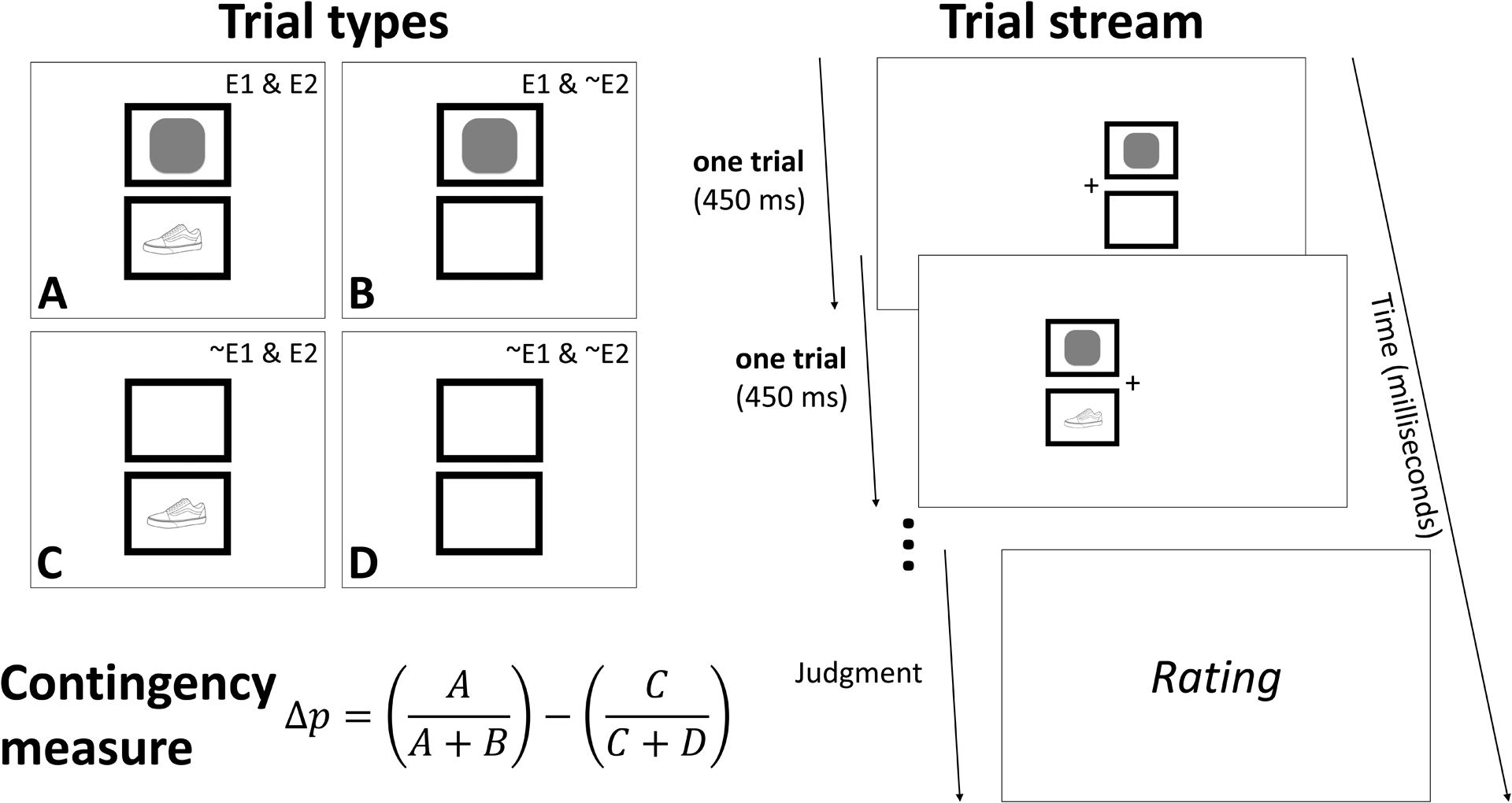
Left-hand panel illustrates the four trial types conceived as relevant for a 2 × 2 contingency between binary events (Allan, 1980). The four squares depict the different instances of the two events E1 (geometric figure) and E2 (object), with their presence and absence varied in the different trial types. Below the squares, the formula for the calculation of the Δp contingency between two binary events is presented as the difference between two conditional probabilities for the occurrence of E2 in the presence of E1 [A/(A+B)] and in the absence of E1[C/(C+D)]. Right-hand panel depicts an example trial stream of two consecutive trials (first a B trial and then an A trial) from the present series of experiments. Participants provided a subjective rating of the relation between the two events (here the rounded square and the shoe). The dimensions are 130 × 130 pixels for the cue and outcome stimuli, and 240 × 190 pixels for the trial marker (TM) borders. Their respective positions are centered at different XY coordinates. For the TM borders: (590, 302) for the top left border, (850, 302) for the top right border, (590, 506) for the bottom left border, and (850, 506) for the bottom right border.

In a typical experiment, participants are exposed to individual trials containing the to-be-associated events, with A trials consisting of either E1 and E2 being presented simultaneously or with one event briefly preceding the second (sequential presentation as might be expected if E1 were a cause of E2), B and C trials consisting of E1 alone and E2 alone, respectively, and D events consisting of ‘trials’ devoid of both E1 and E2. On D trial events, experimenters typically present either a blank screen, or explicit wording of an ‘empty’ trial or trial ‘context’ cues meant to indicate to participants that a trial has occurred in which both events were absent. For example, in a within-subjects study by Wasserman, Kao, Van Hamme, Katagiri, and Young (1996), participants received training with a fictitious fertilizer as E1 and a plant blooming as E2. Across conditions, training was conducted with four different positive contingencies between the events (all with Δp = 0.25), four different negative contingency conditions (all with Δp = −0.25), and thirteen different zero contingency conditions (Δp = 0.0). Participants’ judgements of the conditions appeared to be influenced by participants’ experience with each of the four trial types (also see Allan & Jenkins, 1983; Dickinson & Shanks, 1987; Vallee-Tourangeau, Murphy, Drew, & Baker, 1998). Thus, the presence or absence of both E1 and E2 on each trial influences the strength and direction of the contingency learnt.

A standard model of learning that uses the principle of error prediction, such as that of Rescorla and Wagner (1972), assumes that incremental changes in associative strength accrue as a function of trial frequency. Trial duration can be modelled by assuming an arbitrary temporal unit and that increasing duration increases the number of those units, and that is what we have done in Figure 2. So that at least in the case of a one or zero event trial (i.e., B, C, or D), a 200-m exposure to an event should be half as effective as 400 ms. Using the Rescorla-Wagner theory, we modelled the changes in associative strength for changes in frequency and duration for each of the four trial types and illustrate them in Figure 2 panel a. Clearly, the model predicts the pattern of results for the overall contingency analysis described above. Increased associative strength is predicted for increases in either frequency or duration to A and D trials, while decreased associative strength is predicted for increases in B and C trials.

Figure 2.

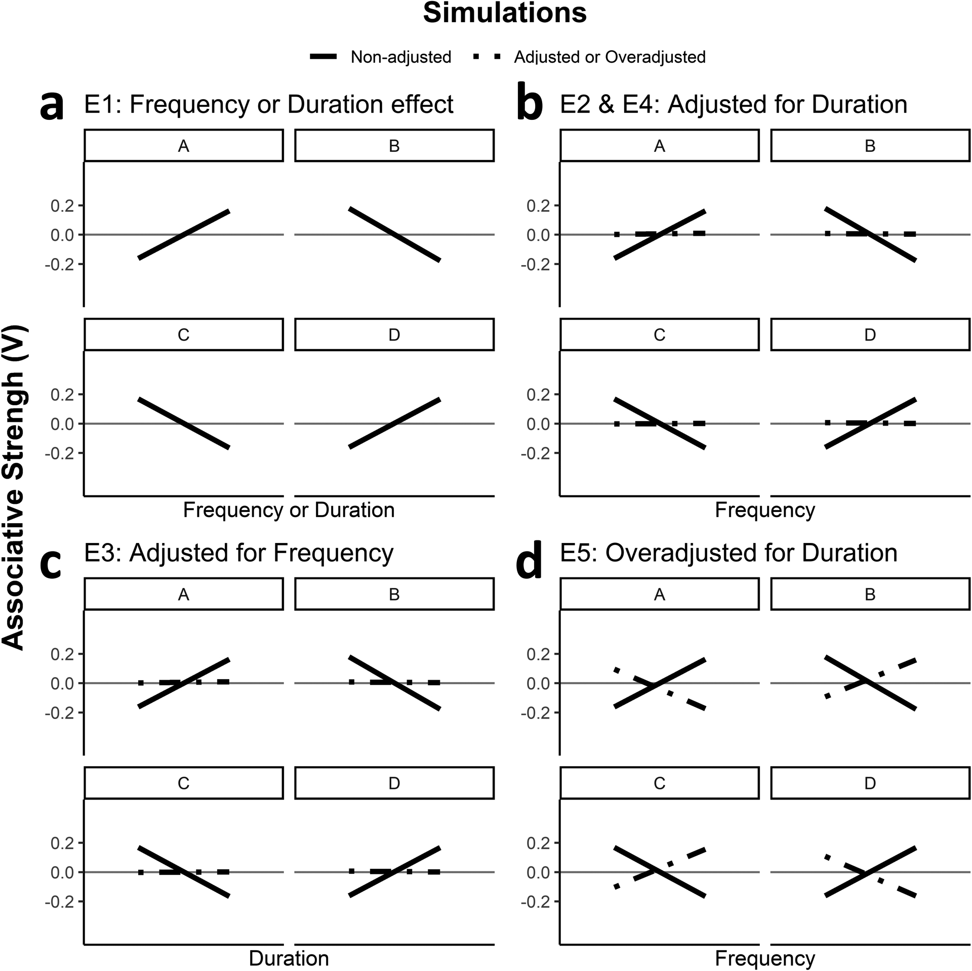
Predicted associative strengths for each experiment (E) based on the Rescorla-Wagner (1972) model. Panel a represents the predicted change in associative strength between two events following changes in either frequency or duration of each of the four type of trial independent of the any changes in the other type of trial for Experiment 1. Panel b predictions for Experiment 2 and 4. Panel c predictions for Experiment 3, and Panel d predictions for Experiment 5.

Although human judgements track the output of the Δp metric, relatively consistent deviations from Δp are commonly observed. One hypothesis to address these deviations from the simple Δp is that the different types of trial information are weighted differently for judgements (e.g., Kao & Wasserman, 1993; Wasserman et al., 1993; White, 2004); that is, Δp = (W_AA/[W_AA+W_BB]) - (W_CC/[W_CC+W_DD]), where W_i is the relative weight of trial type i. Based on fits to data, Kao and Wasserman suggested that judgements are most heavily influenced by the number of A events (i.e., pairings), somewhat less by B and C events, and least by D events; that is, W_A > W_B ~ W_C > W_D. This is consistent with the general observation that the presence of an event has greater influence than its absence when learning an association. This principle is also seen in discrimination learning (e.g., Jenkins & Sainsbury, 1970; Uengoer, Koenig, Pearce, & Lachnit, 2012). In those experiments, a cue configuration that signals an outcome is easier to learn about than a cue configuration that signals the absence of the outcome. Assuming that the perceptual qualities of these different experiences (i.e., presence vs. absence) influence how they are processed begins to explain the observed departure from a normative or a purely informational account of contingency judgements (i.e., W_A = W_B = W_C = W_D). Regardless of theoretical perspective, the perceived relatedness between E1 and E2 should increase with selective increases in the frequency of A trials because these trials are evidence of a positive association between the two events. In contrast, either E1 alone or E2 alone is evidence against a positive association; thus, selective increases in the frequency of B and C trials reduce the perceived relatedness between E1 and E2. Moreover, the absence of both events is consistent with the view that they are related, although this latter case by itself is clearly insufficient evidence of a positive relationship between a cue and an outcome (e.g., Wasserman & Miller, 1997).

Previous research investigating the effects of frequency of A, B, C, and D trials often confounded frequency with cumulative duration of the A, B, C, and D trials, respectively. For example, a common experimental method is to allow self-pacing of the trial presentations by participants; therefore, participants view trial events for unsystematically variable durations. In other experiments, the experimenter defines the durations, but as the number of a given trial type increases, so too does cumulative exposure time to that type of trial. Little analysis has been conducted on the relative roles that trial duration and trial frequency play in the perception of contingency. Given that these trials happen in real-time, a test of the relative contributions of trial frequency and trial duration to the perceived association requires experimental control over the amount of time that each trial is presented as well as how often it is presented. It is clear that simple control of exposure to the trials requires removing the opportunity for the participant to pace the trials. Additionally, the durations and frequencies of different types of trials need to be varied by comparable proportions to compare the relative roles of frequency and duration of the different types of trials on the perceived contingency. If total trial duration is crucial for acquisition, then there is little possibility of speeding up learning because increases in duration of exposure would lengthen total training time. However, if frequency is a critical variable, then it might be possible to enhance learning without lengthening total training time by shortening trial duration while increasing trial frequency.

Even more challenging for any attempt to compare trial frequency and duration is the question of how to manipulate the frequency and duration of trials on which both events are absent (i.e., D trials). One of the reasons to believe that D trial duration is particularly relevant comes from the many demonstrations of the previously mentioned ‘trial spacing effect,’ in which longer ITIs, periods in which no events occur, are often found to result in superior learning and retention (e.g., Wickelgren, 1972). Unless something marks the occurrence of individual trials, a long inter-trial period might be processed as one long ITI event or multiple shorter sequential ITI events. For example, Gibbon’s (1977) scalar expectancy theory (SET; Gibbon, 1977) assumes that a pace-maker (or ‘internal clock’, see Treisman, 1963) mechanism underlies timing estimation. In this framework, animals are assumed to experience an ITI as a series of discrete states resulting from the parsing of time between A, B, and C trials into a sequence of D trials (e.g., Buhusi & Meck, 2005). Of course, this ambiguity also exists with respect to A, B, and C type trials if nothing (including D trials) separates otherwise identical trials (e.g., two A trials in immediate succession). The present experiments used a procedure explicitly designed to circumvent this issue.

Streaming Procedure

In light of the evidence that association learning between paired events may relate to event rates rather than event frequencies, we employed a preparation that was specifically developed to circumvent the time constraints of conventional contingency learning procedures. Crump et al. (2007) described their task as involving the rapid presentation of events within relatively short ‘trial streams’ in which trials are presumably parsed by participants isomorphic with the experimentally manipulated trial frequencies. Participants viewed 60 trials of training over the course of 12-s. Each trial depicted one of the four types of trials (A/B/C/D) relevant for the relation between two geometric figures, a square and a circle, presented on a computer screen (simultaneously on A trials). The results from participants’ contingency judgements and trial frequency estimates suggested that participants perceived and learned the relations between the stimuli with ease, even with trial durations as low as 100 ms. Participants reported a stronger E1-E2 contingency after the streamed trials in the two Δp-positive conditions than the two Δp = 0 conditions. Note that while an interpretation of these results in terms of overall contingency based on trial frequencies is consistent with the findings, it is also the case that accumulated trial durations or subsets of trial frequencies might have controlled participants’ judgements. For instance, in the experiment described here, the frequency and summed durations of A trial events in the two Δp-positive contingency conditions was greater than the frequency and summed durations of A trial events in the two Δp = 0 conditions; therefore, frequency of A trials, summed durations of A trials, or both may have been responsible for differences in judgements rather than sensitivity to the number of each of the four types of trials.

Across a wide range of contingencies, Allan, Hannah, Crump, and Siegel, (2008) found relatively accurate learning of the contingencies between pairs of events that may have encouraged fast processing or different types of processing (i.e., emoticons that have a social value rather than geometric figures) and events indicating motivational shifts (i.e., financial rewards). The task has also been used for the training of more complex contingent relations including those involving an instrumental component (Hannah, Allan, & Siegel, 2007) and stimulus interaction experiments with multiple stimulus relations (Hannah, Crump, Allan, & Siegel, 2009; see also Darredeau, Baetu, Baker, & Murphy, 2009; Laux, Goedert, & Markman, 2010). In the present experiments, we used Allan’s streaming procedure to assess how humans learn contingent relations, specifically whether frequencies and/or durations of the different trial types are critical for these learning effects.

Experiment 1a

Experiment 1 was designed to accomplish two goals: (1) to dissociate the effects of the frequencies of A, B, C, and D trials from the effects of their duration, and (2) to assess a modification to the streaming procedure that would allow equivalent manipulations of A, B, C, and D trials. In the first experiment, we sought to dissociate trial frequency from trial duration by presenting multiple conditions across which frequency or duration of one trial type at a time was varied, while equating the frequencies and durations of the other trial types. For instance, illustrated in the experimental design presented in Table 1, in a baseline Δp = 0 contingency condition, participants were exposed to 36/36/36/36, A/B/C/D trials, pseudo-randomly ordered, with all trial durations being 800 ms. However, in a manipulation of A trial frequency, the Fewer-A condition contained 9/36/36/36 trial events, whereas the Many-A condition was trained with 144/36/36/36. The comparison here was whether increasing the frequency of A trials by factors of four would result in increased judgements of association between the two events when the same trial duration of 800 ms was maintained for all trial types. Notice that Fewer-A and Many-A also have shorter and longer total duration of A trials, so two conditions were included in which only the duration of all A trials was manipulated. In the Shorter-A condition, the 36 A trials were reduced to 200 ms each (the same total time in A as 9 A trials for 800 ms each), and in the Longer-A condition the 36 A trials were increased to 3200 ms (the same total time in A as 144 A trials for 800 ms each), with the same 36 trials of 800 ms duration for B, C, and D trials. Hence, the variation in the duration of A trials not only assessed the influence of duration of A trials but also controlled for the changes in total duration of A trials when only the frequency of A trials was varied. In sum, the effect of using these values of frequency and duration was to maintain the duration or frequency, respectively, of A trials across conditions, with the variation of each variable being by the same factor of four. The Shorter-A and Fewer-A conditions each consisted of 7200 ms of total exposure to A trials, and the Longer-A and Many-A conditions each consisted of 115.2 s of total exposure to A trials. In this first experiment, we used the same reasoning to also independently alter training experience with the other three trial types (i.e., B, C, and D trials) in sets of other similarly varied conditions. However, note that the Figure 2 Panel a illustrates the prediction of the Rescorla-Wagner (1972) associative model; increasing either frequency or duration of a given trial type while holding the other trial types constant is predicted to have a similar effect.

Table 1.

The conditions in Experiments 1a and 1b: Event-Event conditions varied in terms of frequency and duration of trials from a baseline condition with 36 trials presented for 800 ms. From this baseline condition frequency and duration were varied by a factor of ¼ for the Fewer (9) and Shorter (200 ms) conditions or by 4 for the Many (144) and Longer (3200 ms) conditions.

		Duration (ms)
		200	800	3200	200	800	3200
Frequency	9		Fewer A			Fewer B
	36	Shorter A	Baseline	Longer A	Shorter B	Baseline	Longer B
	144		Many A			Many B
	9		Fewer C			Fewer D
	36	Shorter C	Baseline	Longer C	Shorter D	Baseline	Longer D
	144		Many C			Many D

Note: Baseline was a single control condition used to compare across the manipulations of the four trial types. In the Baseline condition, each trial type, A, B, C and D, was repeated 36 times at 800 ms. In the other conditions, Frequency or Duration of one type of trial (A, B, C, or D) deviated from the Baseline condition.

A second modification to the streaming procedure implemented here relates to an experimental ambiguity of the D trials described previously (Crump et al., 2007; Maia, Lefevere, & Jozefowiez, 2018). As trials are often randomised, any repeated presentations of the same type of trial in immediate succession might be perceived as either multiple separate trials or a single longer duration trial. Because trials are streamed rapidly, the discrimination between sequential trials of the same type based on duration alone would be difficult. One solution is to introduce an ITI which might be expected to solve this problem; however, the ITI in which no events occur would be indiscriminable from D trials in which neither event occurs. Prior investigators (e.g., Crump et al., 2007) addressed this problem by briefly presenting a blank screen (i.e., an absence of the context of A, B, C, and D trials), but it is unclear whether the blank screen without the cue or outcome was perceived as distinctly different from a D trial. We sought to overcome this problem with two procedural changes. One was to present each trial with a trial marker (TM) that consisted of a pair of identical, vertically aligned rectangular frames to signal trial times and spaces in which the two events might or might not appear as shown in Figure 1 (see Murphy & Baker, 2004 for the use of a TM in Pavlovian conditioning). On each trial, the top frame might contain a shape (E1) and the bottom frame might contain a line drawing of an object (E2). During A trials, the top frame contained a shape and the bottom frame contained a drawing. During B trials, the top frame contained a shape and the bottom frame was empty. During C trials, the top frame was empty and the bottom frame contained a drawing. During D trials, both frames were empty. Although this modification may highlight the presence or absence of either stimulus, it does not eliminate the problem of how participants might parse repeated trials of the same type without using some form of transition between trials. To avoid the potential confound of participants’ perceiving extra intertrial time as D trials, a second procedural change was to present trials in an alternating left-right position in the two locations on the screen as depicted in the right panel of Figure 1. In this manner, each trial of any given type was the same duration, and immediately repeated trial types always appeared in different locations. This permitted parsing of sequential trials without conventional ITIs, which would have confounded the potential counting of D trials.

Methods

Participants.

Experiment 1a involved recruitment of 43 university students (33 females and 10 males) who received course credit for their participation. Sample size was based on the initial study using the streaming procedure, specifically Crump et al. (2007), who reported sensitivity with n = 37. The mean age was 25.16 (SD = 8.1) years, ranging between 14 and 50. Due to the rapidly changing images on the screen, recruitment postings and the informed consent form excluded potential participants who had a propensity for convulsions. They were all students at the University of Canterbury in New Zealand. Experiment 1a was reviewed and approved by the Institutional Review Board of the University of Canterbury. All subsequent experiments were reviewed and approved by the Institutional Review Board at the State University of New York at Binghamton.

Design.

A fully within-subject design was used in which each participant experienced 17 different contingency conditions (see Table 1) presented in random order. A Baseline condition in which there were the same number (i.e., 36) of each trial type (A/B/C/D) with each trial lasting 800 ms was contrasted with two different trial-type manipulations, Frequency (Fewer or Many) and Duration (Shorter or Longer). Thus, there were four conditions within each of the four trial types (A, B, C, and D) plus the Baseline condition for a total of 17 experimental conditions, all preceded by one Warmup condition. Each condition involved learning the relation between a unique pair of E1 and E2 stimuli, with E1 drawn randomly without replacement from a list of black and white symbols, and E2 drawn from a list of black and white line drawings of commonplace objects.

Procedure.

The computer tasks were programmed in E-Prime 2. Each participant was exposed to a Warmup condition in which 144 total trials (36 each of A, B, C, and D) were presented in nine successive blocks, each consisting of four presentations of each of the four trial types presented in random order within a block, with each trial lasting 800 ms. The Warmup contingency condition was the same as the Baseline contingency, but with a different pair of stimuli, E1 and E2. The remaining 17 conditions, including the Baseline condition, were then presented in random order.

Within the conditions that differed in Frequency, all trials were 800 ms as in the Baseline condition, but the frequencies were changed. In each Fewer condition, 117 total trials were presented in nine blocks, with the trial type presented less frequently presented only once per block. For example, the Fewer-A condition received 1 A, 4 B, 4 C, and 4 D trials in each of the nine blocks. In the Many-A condition, 252 total trials were presented in nine blocks, with A trials being presented four times as often as the other trial types for a total of 144 A trials. So, the Many-A condition included 16 A, 4 B, 4 C, and 4 D trials in each of the nine blocks.

Within the conditions that differed in Duration, the frequencies of each trial type were consistently 36 in number as in the Baseline condition, but the durations were changed. In each Shorter condition, the trial type in focus was presented for a reduced duration of 200 ms and in each Longer condition the trial type in focus was presented for 3200 ms, whereas the other three trial types were consistently 800 ms long. Thus, the Warmup and Baseline conditions presented an uncorrelated relation between the two events, as the probability of one stimulus being presented with the other stimulus was 36/(36+36) = 0.5, whereas the probability of either event without the other was the same, 36/(36+36) = 0.5. Consequently, the objective contingency was Δp = 0.5 – 0.5 = 0. Trial order within a block was randomly selected without replacement for each of the 17 experimental conditions. The 18 cues and 18 outcomes were organized into 18 pairs (i.e., a cue and an outcome consistently yoked for all participants) and were randomly selected without replacement for the 17 experimental runs for each participant, with a common E1-E2 pair used for the Warmup condition. The use of the terms ‘Cue’ and ‘Outcome’ here need to be qualified as in Experiment 1a (and 1b) they were presented simultaneously on A type trials. The terminology of cue and outcome reflects only the wording of the question used to assess contingency learning. Simultaneous presentation of the two stimuli was used to avoid the ambiguity that sequential presentation would have created on B and C type trials; for example, the first part of a C type trial without a ‘cue’ would have been indistinguishable from a D-type trial. The dimensions for each stimulus event were 130 × 130 pixels, and 240 × 190 pixels for the rectangular trial marker (TM) borders (see left panel of Figure 1). Their respective positions were centered at different XY coordinates. For the TM borders: (590, 302) for the top left border, (850, 302) for the top right border, (590, 506) for the bottom left border, and (850, 506) for the bottom right border. The cue and outcome stimuli were centered inside the TM rectangles. Throughout each training condition, a small fixation cross was consistently present at the center of the screen where the corners of the four rectangular TMs approached each other.

The dependent variable was ratings of the relation between the two events. Participants were asked to judge the contingency between the ‘cue’ and ‘outcome’ following each of the 17 experimental runs (consisting of 117, 144, or 252 trials/condition). The total session time for the experiment was approximately 50 minutes.

Before participating in the experiment, all participants were required to complete an informed consent form, turn off their mobile phones, read a series of instructions presented on the computer screen, and provide demographic information (age and gender). The instructions informed participants that they “… will be watching numerous series of rapidly presented shapes and drawings. After each series, a question screen will appear and you will be asked to rate the degree of relatedness between the shape and drawing on a scale from −10 to +10. Please keep your eyes on the cross in the center of the screen. A strong positive rating should be given when the shape and drawing are always presented together and when one is absent the other is also absent. A strong negative rating should be given when the shape is always presented without the drawing and the drawing is always presented without the shape.” Any participant who provided the same rating on all 17 experimental runs was scheduled to be eliminated from the experiment, but in practice, this never occurred in this or any of the subsequent experiments.

Statistical analysis:

A linear mixed model (LMM) analysis with a subject random intercept was conducted. The LMM analysis was performed in R (R Core Team, 2019) using the function lmer() from the package lme4 (Bates & Machler, 2014). To obtain ANOVA’s F scores and p values from lmer(), the package lmeTest (Kuznetsova, et al., 2017) was used. ANOVAs were generated by passing the model through the anova() function from R-base. For the Full model, the LMM predicted ratings (−10 to 10) using eight predictors: A, B, C, and D, from Frequency and Duration (i.e., 4 × 2). The form of the Full model was as follows:

$${\mathit{\text{rating}}}_i=\left({\beta }_0+{\beta }_{0,j}\right)+{\beta }_1*f{A}_i+{\beta }_2*f{B}_i+{\beta }_3*f{C}_i+{\beta }_4*f{D}_i+{\beta }_5*d{A}_i+{\beta }_6*d{B}_i+{\beta }_7*d{C}_i+{\beta }_8*d{D}_i+{\epsilon }_i$$ (eq. 1)

where i is the ith data observation and j the jth subject, β_0,j and β₀ are intercepts for the random effects of participant and order of conditions, and ε_i (error) ~ N(0,σ), and the f or d before the A, B, C, or D refers to frequency (f) or duration (d), respectively. By feeding the model only with the actual values of frequencies (9, 36, or 144) and durations (200, 800, or 3200), the model was blind to the conditions. The regressors were factors/categories, this means that they were imputed using dummy variables and the reference category for all of the regressors were the baseline, that is, 36 for frequency and 800 for duration. We did not use conditions as regressors. So we did not need to duplicate the baseline condition. As regressors we used the actual frequencies and durations. The R scripts code used for statistical analysis, plots, and data files (for all the experiments) are available online: https://github.com/santiagocdo/ABC_paper (instructions provided in readme file). The threshold for rejecting the null hypothesis, α, was established as 0.05. The results from each Frequency and Duration model, which included either the three levels of the factor frequencies or three levels of duration of each trial type as predictors, were obtained. A model comparison between the Full, Frequency, and Duration models to assess the fit between the data and the models was also performed.

Results

The mean judgements, and individual ratings, for each of the 17 contingencies are presented in Figure 3 with the Frequency manipulation presented in the four left-hand panels and the Duration manipulation in the four right-hand panels. Generally, judgements were influenced by trial frequency for A, B and C trials, but not by D trials (i.e., the absence of both stimuli). Trial duration showed smaller but reliable effects for A, B, and D trials, but not C trials. Next, we present the F scores and p values for individual factors. A summary of the Full model with effect sizes is presented in Table S1 of the Supplementary Materials.

Figure 3.

Contingency judgement data from Experiment 1a panel a shows the trial Frequency effect, and panel b shows trial Duration effect. The black shapes represent the means with the 95% CIs computed by a bootstrap method (using stat_summary (fun.data = “mean_cl_boot”) function in ggplot2 package; Wickham, 2016). The black lines are linear fit (using geom_smooth(method = “lm”) from ggplot2). At the top of each subplot, the significance of the F-score from the Full model is indicated, where *** is p < 0.001, * is p < 0.05, and nonsignificant (ns). Individual participant points and lines are added with a y-axis jitter in grey.

Full model:

In the Full model with all eight predictors, Frequency was reliable for A trials (F[2, 688] = 49.40, p < .001), B trials (F[2, 688] = 25.45, p < .001), and C trials (F[2, 688] = 27.20, p < .001), but not D trials (F[2, 688] = 1.22, p > .1). However, Duration was also related to judgements for A trials (F[2, 688] = 3.06, p < .05), and B trials (F[2, 688]) = 3.96, p < .05), and D trials (F[2, 688] = 3.55, p < .05), but not C trials (F[2, 688] = 1.93, p > .1).

Frequency model:

The analysis of the separate model testing trial Frequency only found significant effects for frequency of A trials, (F[2, 688] = 46.43, p < .001), B trials, (F[2, 688] = 29.05, p < .001), and C trials, (F[2, 688] = 29.90, p < .001), but not D trials (F[2, 688] = 1.66, p > .1).

Duration model:

The analysis of the separate model testing trial Duration found reliable effects of duration of A trials (F[2, 688] = 3.09, p < .05) and D trials (F[2, 688] = 3.46, p < .05), but not of B trials (F[2, 688] = 2.78, p > 0.05) nor C trials (F[2, 688] = 1.48, p > .1). Figure 3 illustrates the significant effect of D trial duration, with the effect represented by this F score including the Baseline condition. This F value is based on the D duration variable, which is a factor of 3 levels: 200, 800, and 3200. For this 3-level variable the model uses 800 (i.e., baseline) as comparison, and it creates two dummy variables 200 and 3200. However, notice that the regression line looks quite flat; indeed, the statistical analysis found that the slope was not significant.

Model comparison:

When we compared the Full model (deviance = 4162.2) against the Frequency model (deviance = 4177.9) there was a statistically significant difference, χ²(8) = 15.68, p < 0.05, i.e., lower deviance for the Full model; however, ΔAIC = 0.32 and a Bayes Factor (BF) approximation (Wagenmakers, 2007) > 100 support a better fit for the Frequency model against the Full model. Similarly, the difference between the Full model (deviance = 4162.2) and the Duration model (deviance = 4345.6) was statistically significant, χ²(8) = 183.39, p < 0.001, and ΔAIC = −167.39, BF > 100 supporting the Full model. Comparing the Frequency model against the Duration model found a better fit for Frequency (ΔAIC = 167.7, BF > 100), supporting the Frequency model over the Duration model. No likelihood ratio was calculated because these models are nested within the Full model but not within each other. In summary, the comparison of models suggests that Frequency is a better explanation of ratings than is Duration. Moreover, the Frequency model is better and more parsimonious than the Full model, which is not the case for the Duration model.

Experiment 1b

Experiment 1b sought to test the replicability of the effects found in Experiment 1a using an online testing method. In this experiment the instructions, design and analysis were as similar as possible to Experiment 1a, except participants were recruited from Amazon’s Mechanical Turk (MTurk) online crowdsourcing system and tested on their own computers. We present Experiment 1b as a near replication of Experiment 1a both to assess the reliability of the results of Experiment 1a and to examine the consistency of the data between participants tested on computers in a conventional university laboratory setting and participants tested online with Amazon’s MTurk platform.

Methods

Participants:

Forty-three participants (18 females, 22 males, 1 non-binary, 2 preferred not to say), with a mean age of 33.6 (SD 7.84; range between 22 and 49), were recruited online via Amazon’s Mechanical Turk and compensated with US $4.00 for completion. Recruitment was restricted to users who were reported by Amazon as living in the United States and not having previously participated in any similar experiment from our laboratory. Previous studies in learning and cognition have reported strong agreement in many (but not all) basic cognitive tasks between traditional laboratory procedures and being conducted on MTurk (e.g., Crump, McDonnell, & Gureckis, 2013). The procedure used rapid streaming of images, so participants who self-identified as having a history of seizures or being younger than 18 or older than 50 years were excluded. These qualifications were applied in all subsequent experiments.

Procedure:

The online version of the program was written in HTML, with the participants in Experiment 1b experiencing stimuli and tasks nearly identical to Experiment 1a. The online version of the procedure was as similar as possible to the in-laboratory procedure except for the following differences. Participants were instructed to not use a mobile device to perform the task. For computer performance reasons, they were also asked to not use Internet Explorer. Participants were instructed to respond to all questions (e.g., cue-outcome contingency judgements) in less than 10 s and were excluded from the experiment if they ever delayed their responses by more than 20 s. Participants were permitted to take short breaks (up to five minutes) between conditions after rating the most recently experienced condition. In order for the images to display correctly on various computer monitors, the width of each cue and outcome was 216 pixels × 176 pixels (W × H), including a 20-pixel wide, black border that served the trial marker on all trials. All stimuli were presented in a centrally arranged 462-pixel × 332-pixel rectangular area, with a centered fixation cross highly similar to the one in the right panel of Figure 1.

Results

The mean judgements of association between the two events from the 17 different contingency conditions are shown in Figure 4 and provide a pattern very similar to the results of Experiment 1a. Frequency seems to influence judgements more than duration. See the Full model summary in Table S2 in Supplementary Materials.

Figure 4.

Contingency judgement data from Experiment 1b panel a shows the manipulation of trial Frequency, and panel b shows trial Duration effect. Error bars = 95% CIs. At the top of each subplot, the significance of the F-score from the Full model is indicated, where *** is p < 0.001, ** is p < .01, * is p < 0.05, and non-significant (ns). Individual participant points and lines are added with a y-axis jitter in grey.

Full model:

The effects of frequency of A trials (F[2, 688] = 47.74, p < .001), B trials (F[2, 688] = 21.92, p < .001), and C trials were significant (F[2, 688] = 16.01, p < .001), but D trials were not (F[2, 688] = 0.00, p > .1). Similarly, the effect of duration of A trials (F[2, 688] = 5.62, p < .01), B trials (F[2, 688] = 8.13, p < .001), and C trials were significant (F[2, 688] = 4.40, p < .05), but D trials were not (F[2, 688] = 0.33, p > .1).

Frequency model:

For the Frequency model, we found an effect of frequency of A trials (F[2, 688] = 46.11, p < .001), B trials (F[2, 688] = 21.65, p < .001), and C trials (F[2, 688] = 16.25, p < .001), but not of D trials (F[2, 688] = 0.00, p > .1).).

Duration model:

For the Duration model, we found an effect of duration of A trials (F[2, 688] = 4.55, p < .05), B trials (F[2, 688] = 7.63, p < .001), and C trials (F[2, 688] = 4.12, p < .05) , but not D trials (F[2, 688] = 0.32, p > .1).

Model comparison:

When the Full model (deviance = 4315.1) was compared with the Frequency model (deviance = 4356.7), a significant difference was found, χ²(8) = 41.57, p < 0.001. The Full model had lower deviance, ΔAIC = −25.6 in favour of the full model, but when correcting for complexity a BF > 100 was found, supporting the Frequency model. Similarly, the Full model (deviance = 4315.1) better fit the data than did the Duration model (deviance = 4475.2), using the likelihood ratio test, χ²(8) = 160.06, p < 0.001, and the other two indicators, ΔAIC = −144.0.6, BF > 100, also supported the Full model. Finally, we compared the Frequency model against the Duration model and obtained evidence supporting the Frequency model, ΔAIC = 118.5, BF > 100. In summary, as in Experiment 1a, the Frequency model seemed to be the most parsimonious model to explain the data; however, duration still showed some explanatory power that was always in the same direction as the frequency manipulation (e.g., the effect of Longer was always in the same direction as Many). A similar analysis conducted with pooled data from Experiments 1a and 1b provided similar support for the effect of Frequency (see Table S3 in Supplementary Materials).

A backward elimination of non-significant fixed and random effects using a step-wise algorithm (Kuznetsova, et al., 2017) was applied to the Full model of the pooled data (see Table S3). This algorithm selected the factor with the worst predictive value, creating a Reduced model without it, comparing the Full against the ith Reduced model, and repeating this until there was no factor that with its elimination improved the final model significantly (see more details in Kuznetsova, et al., 2017). The final model resulted in the elimination of both D frequency and D duration factors, suggesting little if any effect of our manipulations of D trials.

Discussion

Experiment 1 provides the first demonstration of the impact of trial type on contingency judgements in which there was a dissociation between frequency and duration in a situation in which the ranges of variation were matched (i.e., here by a factor of 16). The frequency with which both stimuli were presented together (A trials) or either stimulus was presented alone (B and C trials) had an effect on contingency judgements that was consistent with the previous literature on the experimental manipulation of trial frequencies (e.g., Wasserman et al., 1996) and consistent with the prediction reported in Figure 2 panel a. Interestingly, there was no indication that frequency of D trials had an effect on judgements. The D trials are logically as informative as the other types of trials and, from the perspective of theories of learning, the D trials provide exposure to and extinction of the trial context. Yet, manipulations of D-trial frequency and duration produced little change in perceived contingency in the present preparation. However, as previously mentioned, prior research has found that although Δp is a good descriptor of contingency judgements, weighted Δp is a better one, where the weight of A trials is larger than weights of B and C trials, which in turn are larger than the weight of D trials (e.g., Kao & Wasserman, 1993; Wasserman et al., 1993; White, 2004). Thus, the present failure to observe an effect of either the frequency or duration of D trials more likely reflects a D-trial weight too small to be detected in the current preparation rather than simply the absence of any effect of D trials in the current preparation. Other research in our laboratory lends support to this account with respect to the weight of D trials (Castiello et al., manuscript in preparation). An alternative perspective is that D trials are effectively ITIs and, when these trials are made longer, they support better learning of the content of the non-empty trials (i.e., A, B, and C trials).

Experiment 1 did find evidence of a small to very small (see Table S3) effect of A, B and C duration trials in the direction anticipated by changes in Δp calculated based on exposure times to the four types of trials, as opposed to frequencies. In this framework, an increase in exposure to one event without the other (i.e., B or C trials) is consistent with a decrease in the overall contingency. Although this effect was small when the duration of B or C trials was manipulated, it consistently occurred across conditions in which the same number of experiences of B or C (i.e., frequencies) were presented. Two very similar versions of the experimental design were conducted in different environments (i.e., conventional cubicles and MTurk) with similar results. An analysis of the complete data set found highly similar patterns of findings (see Supplementary Table S3).

It is worth noting that the manipulations of frequency, unlike the manipulations of duration, were confounded in Experiment 1, thereby undermining the strength of the evidence and conclusions concerning the effects of trial frequencies. Specifically, the manipulation of frequency in the Fewer and Many conditions involved decreasing and increasing, respectively, trial frequency, but also had the effect of decreasing and increasing the total duration of exposure to the trial events (i.e., Fewer conditions were exposed for a total of 9 trials of 800 ms each and Many conditions were exposed for 144 trials of 800 ms each). Thus, while manipulations of duration were not confounded, manipulations of frequency were confounded because increases (or decreases) in trial frequency also increased (or decreased) total time in the presence of the A, B, or C trials (see Table S3).  One might argue that the absence of effect of duration indicates that it was actually the number of A, B, and C trials and not the accompanying change in total duration of exposure to A, B, or C trials that produced the observed changes in contingency judgements, a finding that would be inconsistent with recent experiments looking at a similar relationship between exposure and memory (e.g. Melcher, 2001). However, there are at least two problems with this argument.

First, the duration and frequency of B were both significant factors, Frequency of B trials (F[2, 688] = 21.92, p < .001) and Duration of B trials (F[2, 688] = 8.13, p < .001). However, part of the observed effect of Frequency of B trials might have been due to altered B trial duration. This means that the true effect of the Frequency of B trials might have been overestimated, with the difference between ‘pure’ Frequency effects and Duration effects being substantially smaller than suggested above. The same might be true for A and C trials, although the effects of duration of A and C trials were far smaller than the effect of Duration of B trials. For D trials, the nonsignificant effect of Duration was actually in the opposite direction from that of Frequency of D trials (the latter of which was consistent with Δp). But for A, B, and C trials, the inherent changes in overall trial Duration accompanying changes in trial Frequency might have appreciably contributed to the observed effects of Frequency of A, B, and C trials.

The second problem is that the changes in overall duration of A, B, and C trials that accompanied changes in frequency of these trials were distributed differently across the training stream than were the changes in duration of the A, B, and C trials when the durations of the A, B, and C trials were explicitly manipulated. Changes in duration in conditions Shorter and Longer resulted in different individual trial lengths, whereas the frequency manipulation always used the same duration. This asymmetry may have masked the effects of Duration and perhaps enhanced the effects of Frequency.

Experiment 2

Experiment 2 was conducted to assess the contributions of and possible interactions between changes in the cumulative durations of A, B, and C trials when we manipulated frequency of A, B, and C trials while holding constant the duration of individual trials in the Frequency conditions. In this experiment, the frequencies of A, B, and C trials were manipulated while the durations of the A, B, and C trials were inversely adjusted (Adj), so the changes in frequency were not accompanied by changes in the total trial duration of the manipulated trial type. Figure 2 panel b illustrates the predicted effects on learning derived from the Rescorla-Wagner (1972) model for the effect of adjusting trial duration while modifying trial frequency. Increased frequency is predicted to enhance the impact of each trial type. The Non Adjusted conditions are similar to those used in Experiment 1 and are predicted to result in changes in associative strength consistent with the Δp model. However, participants in the Adjusted conditions experienced changes in trial frequency with trial duration being inversely modified. Therefore, if the strength of the association is a function of the overall duration, then associative strength should be similar in all conditions of a particular trial type. This addresses the confound in Experiment 1 between trial frequency and total duration. The central question was whether the previously observed effects of A, B, and C trial frequency would be diminished by inversely modifying trial duration so that the product of trial duration and trial frequency (i.e., total time of exposure to each of the four trial types) stayed constant across the Adj conditions. We did not vary the frequency or duration of D trials because there had been no consistent effect of frequency or duration of D trials in Experiment 1.

Methods

Participants.

Fifty-one participants (36 female and 15 male) from SUNY-Binghamton with a mean age of 19.2 (SD = 1.27) and an age range between 18 and 24 served as participants in Experiment 2.

Procedure.

The stimuli and method of presentation were the same as in Experiment 1. The changes in the design were to the frequency and duration of trials in each of the 13 contingencies presented to participants within-subjects (see Table 2). The Baseline condition was the same as in Experiment 1 involving 36 presentations of each type of trial, with a consistent 800-ms trial duration. Conditions Few and Many were the same as Experiment 1 and involved either 9 or 144 trials of the manipulated trial type. However, the two corresponding adjusted conditions either used longer duration trials (3200 ms) or shorter duration trials (200 ms). In this way, Conditions Few Adj and Many Adj maintained the same overall trial exposure duration as Conditions Many and Few, respectively, as well as the Baseline condition.

Table 2.

The conditions of Experiment 2 in which Frequency of trials and duration Adjusted for frequency of trials were manipulated.

		Duration (ms)
		200	800	3200	200	800	3200
Frequency	9		Few A	Few A Adj		Few B	Few B Adj
	36		Baseline			Baseline
	144	Many AAdj	Many A		Many B Adj	Many B
	9		Few C	Few C Adj
	36		Baseline
	144	Many CAdj	Many C

Note: Baseline was a single control condition identical to Baseline in Experiment 1, and was used to compare across the manipulations of the A, B, and C trial types. In the Baseline condition, each trial type, A, B, C and D, was repeated 36 times for 800 ms. In the other conditions, Frequency or Duration Adjusted for frequency of one type of trial (A, B, or C) deviated from the Baseline condition.

Statistical analysis.

To model the data, we used an LMM like that used for Experiment 1. But unlike the previous experimental design, here the Baseline condition was part of each trial type’s comparison so that the factors would have the same number of levels. However, to avoid duplicating the data, the first model fit was made omitting the Baseline condition. The Full model is: rating~cells(A, B, C) * frequency(9,144) * adjustead(yes, no), and we included condition order as a covariate and a random subject intercept. We describe the effects from the Full model factors using an ANOVA to obtain F scores for each factor. In addition, we compared the Full model against the Reduced model with Adjusted conditions omitted¹. We then conducted a sensitivity analysis, to determine whether the direction of the effect changed when we added in the Baseline condition (i.e., repeating Baseline condition in each comparison, that is, 3 (cell trial type) × 2 (adjusted, non-adjusted; see Baseline model estimates in Table S4). As post hoc analyses, we explored the individual trial-type effects by fitting models to individual trial types. The detailed sensitivity analysis and its post hoc analysis are presented in Table S4 and S5 in the Supplementary Materials: Experiment 2.

Results and discussion

The top panel of Figure 5 presents the mean judgements of association between the two events and illustrates the effect of frequency for trial types A, B, and C, respectively, found in Experiment 2. For the analysis of frequency without the Baseline condition (i.e., no repeated data inserted into the model), the three-way interaction of Frequency, Adjusted, and Trial type was significant (F[2, 561] = 4.16, p < .05), whereas the covariate, Condition order, was not (F < 1, p > 0.1). The analysis suggested that trial frequency was relevant, but the adjustment for duration was not relevant. The main effect of Frequency (Few-9, Many-144) was significant (F[1, 561] = 6.55, p < .05), but the Adjusted manipulation was not (F[1, 561] = 1.58, p > .1). The effect of the three trial types was significant (F[2, 561] = 11.08, p < .001), but importantly the interaction between Frequency and Adjusted was not significant (F[1, 551] = 0.82, p > .1). However, the interaction between Frequency and Trial type was significant (F[2, 561] = 204.29, p < .001), supporting the observation from Figure 5 that increasing frequencies of A trials increased judgements of association, but increasing frequencies of B and C decreased judgements. The interaction between Adjusted and Trial type was not significant (F[2, 561] = 1.02, p > .1). When Baseline was included, the results did not differ in the direction nor the significance of the effects (see Baseline model estimates in Table S4 in Supplementary Materials). Thus, we observed a reliable effect of the frequencies of A, B, and C trials, but no effect of or interaction with duration adjusted for frequency was seen.

Figure 5.

Judgements of contingency between trained events in the different conditions for Experiment 2 in panel a, and Experiment 3 in panel b. Error bars = 95% CIs.

To compare whether the variable Adjusted played a significant role in the model, we ran a Reduced model without the factor Adjusted (see model comparison). In addition, to assess the effect of the three-way interaction, we analyzed the individual cells’ effects (including Baseline; see Table S5 for post hoc ANOVAs results).

Trial Type A:

We compared a Full model with all three cell types against a Reduced model just for A trial types (i.e., no cells factor was included). The Full model (deviance = 1666) was no better than the Reduced A model (deviance = 1669.8; χ²[3] = 3.76, p > 0.1, but ΔAIC = 2.24 and BF > 100), supporting the Reduced A model. For both models, Frequency was significant (Fs > 120, ps < 0.001) and Condition Order was not (Fs < 1, ps > 0.1). In the Full model for A, neither the Adjusted factor nor the interaction was significant (F[1, 254.8] = 1.54, p > 0.10, and F[1, 254.8] = 3.18, p = .076). These results strongly suggest that the effect on variation in contingency judgements based on the manipulation of A trials is due to the frequency with which those trials are experienced without any significant contribution from trial duration.

Trial Type B:

Similar to A trials, we compared a Full B model (deviance = 1634.7) against a Reduced B model (deviance = 1638; i.e., only B manipulated conditions). The Full B model was no better than the Reduced B model (χ²[3] = 3.35, p > 0.1, ΔAIC = 2.65, and the BF > 100), supporting the Reduced B model. For both models, the Frequency factor was significant (F > 70, p < 0.001) and Condition Order was not (F < 1, p > 0.1). In the Full B model, the Adjusted factor and the interaction were not significant (F[1, 254.8] = 0.15, p > 0.1, and F[1, 254.8] = 1.61, p > 0.1). As seen with the analysis of A trials and consistent with the results of Experiment 2 depicted in Figure 5, trial frequency appeared to be the relevant dimension that contributed to differences across conditions in contingency judgements.

Trial Type C:

We also compared a Full C model (deviance = 1699) against a Reduced C model (deviance = 1706). In this case, the Full C model was not better (χ²[3] = 7.01 p > 0.05, ΔAIC = −1.01); however, a large BF (> 100) supported the Reduced C model. For both models, the Frequency factor was significant (Fs > 40, ps < 0.001) and Condition Order was not (Fs < 1, ps > 0.1). In the Full C model, the Adjusted factor was not significant (F[1, 254.7] = 2.38, p > 0.1) nor was the interaction (F[1, 254.7] = 2.36, p > 0.10).

Model Comparison:

Based on the comparisons between the Full and the Reduced model (non-adjusted for duration), we cannot reject the hypothesis that the two models are equally likely; however, there is evidence in the AICs and BFs that suggest that the Reduced model is better for all three trial types. When Baseline was repeatedly included, the difference between the Full model (deviance = 4926.3) and the Reduced model (deviance = 4941.8) was not significant (χ²[9] = 15.5, p > 0.05, ΔAIC = 2.49, in favor of the Reduced model); when complexity of the models was corrected for, the BF (> 100) strongly supported the Reduced model. However, when the Full model was compared to the Reduced model without the Baseline data, the Full model proved to be better (χ²[6] = 12.64, p < 0.05, ΔAIC = −0.64). But when complexity was corrected for, the BF (> 100), supported the Reduced no-baseline model. This suggests that the most parsimonious models are the Reduced models, which omit adjustment by duration. In summary, the BFs with the BIC approximation (Wagenmakers, 2007) from both model comparisons (duplicated and removed Baselines) support the Reduced models. Consequently, we conclude that the best models are the reduced ones. However, using the likelihood ratio and AIC, when we excluded the repeated Baseline, we could not reject the hypothesis that the two models were equally likely. This suggests that the Full model was slightly better (lower deviance and lower AIC), which is indirect evidence of a small duration effect.

Experiment 2 tested whether the effect of Frequency of A, B, and C trials observed in Experiment 1 was due in part to increasing numbers of any one kind of trial also increasing the total duration in that trial type. Hence, as the number of A, B, or C trials was increased, in the Adjusted conditions the duration of that trial type was reduced proportionately. As was seen in Experiment 1, Frequency of A trials was positively correlated with judgements, and the Frequency of B and C trials was negatively correlated with judgements. When we modified Duration of trials inversely to the Frequency of trials, the effects were slightly reduced, suggesting that the duration of each type of trial does matter but far less so than frequency. Thus, although Duration manipulations had effects on judgements in the directions anticipated by Δp calculated based on cumulative exposure time, these effects of Duration were never statistically significant. Results were consistent with Experiment 1 in which large positive effects of Frequency of A trials and moderate negative effects of Frequency of B and C trials were observed. However, small but significant reductions in these three effects were observed when trial duration was inversely varied so that total time (across trials) in each trial type was held constant. It seems clear that trial duration does have an effect on judgements, but it is much weaker than trial frequency, a result that is in opposition to previous results that suggested either equivalent effects of frequency and duration or minimally an effect of total duration regardless of frequency, albeit in very different preparations (e.g., Melcher, 2001; Rock, 1957).

Experiment 3

One potential concern with our somewhat sanguine conclusions about the Adjusted manipulation is perhaps embedded in the procedural details of Experiment 2. The Adjusted manipulation for Condition Many involved using trial durations as short as 200 ms which might be approaching the limits of human temporal combinatorial cognition in this preparation, particularly with the left/right alternation of stimuli on-screen across immediately successive trials. Notwithstanding the previously published contingency learning research employing trial durations as short as 125 ms (Crump et al., 2009 which demonstrated sensitivity to trial frequency, there are grounds for concern that, for a manipulation designed to assess sensitivity to summation of trial durations, the use of durations as short as 200 ms in Experiment 2 may have introduced a floor effect. This could have obscured an effect of trial duration, thereby masking an effect of adjusted duration in the Many Adj conditions. Therefore, Experiment 3 was conducted to seek an effect of trial duration while avoiding the use of extremely short trial durations. Like Experiment 2, increases in duration of each trial type are predicted to have an effect on contingency ratings consistent with its role in the associative strength modeled in Figure 2 panel c. For instance, increasing the duration of A trials should increase the perception of an association. In the adjusted conditions, the increased duration of trials is compensated by a reduction in frequency. A comparison between the Adjusted and Non-Adjusted conditions provides a test of the effect of duration. Notice that if frequency is the determining variable, then judgements should run in opposition to the predictions of the associative model depicted in Figure 2. The decreased frequency that accompanies the increased duration should result in changes in ratings opposite to the predictions for duration.

In Experiment 3, the minimal (i.e., Short condition) duration was 600 ms and other trial durations were multiples of three with respect to this value. Thus, the Baseline trial duration was 1800 ms and the Long trial duration was 5400 ms. A factor of three (rather than four as in Experiments 1 and 2) was used to avoid very long trials in which the attention of participants would have been more apt to wander. This reduction from a factor of four in the prior experiments to a factor of three in this experiment was based on an examination of the regression of contingency ratings as a function of frequency of A, B, and C type trials in Experiments 1 and 2. In other words, the regression analysis indicated that a change of nine (3 × 3) in Frequency would be sufficient to observe the previously obtained effects of at least frequency. However, the Short Adjusted and Long Adjusted conditions would definitively indicate whether a factor of nine in frequency and duration was sufficient to retain sensitivity to Frequency. In addition to these Short, Baseline, and Long conditions, conditions were included in which the frequency of the trial type in which duration was being manipulated was adjusted so that cumulative training time for the trial type being manipulated was equal to that of the Baseline condition. To fit all of these different conditions into an experimental session that was not impractically long, the Baseline frequency for each trial type was set at 12, and frequency of the trial type being examined in Condition Short Adjusted was 36 and in Condition Long Adjusted was 4, thereby matching the factor of three in durations across the Short, Baseline, and Many conditions. Contingency judgements were collected using the online participant facility MTurk as we had in Experiment 1b. This appeared justified given the high similarity in results between Experiments 1a and 1b (also see Crump et al., 2013). The D trials as well as A, B and C trials were manipulated. In total, participants received one Baseline condition and four conditions (Short, Short Adjusted, Long, and Long Adjusted) for each of the four trial types for a total of 17 conditions as listed in Table 3.

Table 3.

The conditions of Experiment 3 in which Duration of trials and frequency Adjusted for duration of trials were manipulated.

		Duration (ms)
		600	1800	5400	600	1800	5400
Frequency	4			Long A Adj			Long B Adj
	12	Short A	Baseline	Long A	Short B	Baseline	Long B
	36	Short A Adj			Short B Adj
	4			Long C Adj			Long D Adj
	12	Short C	Baseline	Long C	Short D	Baseline	Long D
	36	Short C Adj			Short D Adj

Note: Baseline was a single control condition analogous to Baseline in Experiments 1 and 2, and was used to compare across the manipulations of the four types of trials (A, B, C, and D). In the Baseline condition, each trial type, A, B, C, and D, was repeated 12 times for 1800 ms. In the other conditions, Duration or frequency Adjusted for duration of one type of trial (A, B, C, or D) deviated from the Baseline condition.

Methods

Participants.

Forty-four adults (19 females and 25 males) between 23 and 39 years old with a mean age of 35.9 (SD = 7.2) obtained through MTurk served as participants. One female participant was excluded because their data were lost due to a failure in the program. Thus, 43 participants contributed to the data analysis.

Procedure.

Other than the changes in trials durations and trial frequencies, all procedures were identical to Experiment 1b.

Statistical analysis.

The analysis was very similar to the one performed in Experiment 2, but instead of Frequency and duration Adjusted for frequency as factors, the models had Duration and frequency Adjusted for duration as factors.

Results and discussion

The mean contingency judgements for the 17 conditions of Experiment 3 are presented in the bottom panels of Figure 5. Consistent with findings of Experiment 2, the results with no baseline (i.e., no repeated data included in the model) supported the conclusion that the frequency instead of duration manipulation was the strongest determinant of judgements (i.e., frequency accounted for most of the variance) and the effect of frequency was strongest for A trials, followed by B and C trials. As in Experiment 1, there was no effect of D trial manipulations. In this case, the frequency effect emerges from the Adjusted conditions which have lower frequency and therefore lower ratings.

A Full no-baseline model was created for ratings with Duration, frequency Adjusted for duration, the four trial types, and the respective interactions, with Condition Order included as a covariate. For comparison purposes, a Reduced model without the frequency Adjusted for duration conditions was created. For the Full no-baseline model, the main effects of Duration and frequency Adjusted for duration were not significant (F[1, 645] = 2.13, p > 0.05, and F[1, 645] = 1.99, p > 0.05, respectively). The main effect of Trial type was significant (F[3, 645] = 4.26, p < 0.01). The significant interactions were Duration × Trial type and the three-way interaction (F[3, 645] = 6.38, p < 0.001, and F[3, 645] = 20.73, p < 0.001, respectively). Nothing else was significant. The Full model F scores with replicated Baseline results were very similar (see Table S6 for the effect sizes and model estimates). The Full model (deviance = 3924.1) was better than the Reduced (deviance = 3990.2, χ²[8] = 66.1, p < 0.001, ΔAIC = −50.1, BF > 100), supporting the Full no-baseline model. We found the same direction of effects when we compared the Full baseline model (deviance = 5704.7) against the Reduced baseline model (deviance = 5783.1), with the Full baseline model being better (χ²[12] = 78.452, p < 0.001, ΔAIC = −54.45), but the BF (= 11.12) supported the Reduced model. These comparisons suggest that the Adjusted factor played an important role in explaining the contingency ratings. For both Full models (including or not including Baseline), the three-way interaction of Duration × Adjusted × Cells was significant. In order to explore the interaction, we ran the same model comparison (including Baseline) for each trial type. Individual cells effects were (see post hoc Table S7 in Supplementary Materials):

Trial Type A:

The effect of Duration was significant (F[2, 215.35] = 6.93, p < .001) as was the effect of Adjusted-frequency (F[1, 214.93] = 4.15, p < .05) and the interaction between Duration and Adjusted-frequency (F[2, 214] = 20.98, p < .001). Finally, the Full model (deviance = 1489) was better than the Reduced model (deviance = 1530.7; χ²[3] = 41.75, p < 0.001, ΔAIC = −35.74, a BF > 100), supporting the Full model and suggesting that Adjusted frequency helped the model better explain the data.

Trial Type B:

No main effects were significant (i.e., Duration and Adjusted frequency yielded Fs < 1.5 and ps > 0.05). However, the interaction was significant (F[1, 215.06] = 5.34, p < 0.01). The Full model was better supported than the Reduced model (χ²[3] = 10.476, p < 0.001, ΔAIC = −4.47), but the BF (= 22) suggests that the Reduced model was significantly more likely than the Full model.

Trial Type C:

No main effects were significant (F < 3, p > 0.05). However, the interaction was significant (F[2, 215] = 6.00, p < 0.01). The model comparison favored the Full model in LR test and AIC (χ²[3] = 11.683, p < 0.01, and ΔAIC = −5.68), but when corrected for complexity, the BF (= 12.04) supports the Reduced model.

Trial Type D:

No main effects nor the interaction were significant, and the model comparison was not significant. However, the ΔAIC (= 5.08) and BF (> 100) supported the Reduced model.

A comparison of the models for B and C trial types suggests that it is possible to reject the hypothesis that the two types of models (Full and Reduced) are equally likely. However, the BFs for B and C trial types, as well as D trial types, suggest that the Reduced models are more likely. This is evidence that suggests adjusting the frequency inversely to duration is the main predictor of ratings, but, for B, C, and D trials duration still plays an important role. Nonetheless, it is important to note that for B and C trials not all the model comparisons point in the same direction. We interpret this as a lack of robust evidence in favor of duration or frequency for B and C. Inspection of the post hoc F-scores for the interaction between Duration and Adjusted for A, B, and C supplies indirect evidence against duration and in favor of frequency, which is congruent with the results of Experiments 1 and 2. (For details of the Full baseline model estimates with effect sizes, see Table S6.) Finally, based on the prior experiments, we conclude that Frequency has a stronger effect than Duration, and that the weight of A trials is greater than the weights of B and C trials.

Experiment 4

Although we found consistent evidence for a strong positive effect of frequency of A trials and a moderate negative effect of the frequency of B and C trials, we also found evidence consistent with weak effects of A, B, and C trial durations, but little evidence for any effect of trial D. One of the functional values of contingency learning discussed in the introduction suggested that contingency learning reflects a mechanism that is sensitive to causal variables or at least to variables that allow prediction of future events. Pavlovian conditioning, for instance, demonstrates a strong sensitivity to contingency. Although there is reason to think that learning is usually strongest with simultaneous presentations of the CS and the US (Barnet, Arnold, & Miller, 1991; Rescorla, 1981; Savastano & Miller, 1998), the magnitude and duration of the conditioned response in preparations that assess anticipation of a biologically significant event are ordinarily greater if the CS also precedes the onset of the US by a few seconds. Although the optimal temporal relation for anticipatory responding is dependent upon the particular response in question and the modalities of CS and US, the CS precedes the US in most conventional conditioning preparations (e.g. Schneiderman & Gormezano, 1964). However, in all the experiments presented here so far, we used simultaneous presentation of cues and outcomes which may have interfered with the causal learning processes that support contingency sensitivity when cues precede outcomes (Murphy et al., 2005). One might argue that cues are never presented perfectly simultaneously in the present task because vision is a discrete process. Consequently, a small delay between seeing E1 and E2 (or vice versa) will exist on every A trial (e.g., Friston et al., 2012; Shiferaw et al., 2019), although with little or no systematic temporal ordering of the cues. Previous rapid trial streaming research has used sequential presentations of E1 and E2. For example, Maia et al. (2018) used the streaming procedure with E1 onset preceding E2 onset. Each trial consisted of a 100-ms presentation of the predictive E1, terminating with the onset of E2 which persisted for another 100 ms. The two events did not overlap but did constitute a sequential presentation, with trials separated by a 100-ms ITI that was differentiated from a D trial by an absence of a trial marker (see Murphy & Baker, 2004 for the use of trial markers in Pavlovian conditioning). They found a differential sensitivity between positive and negative objective contingencies, and suggested that the difference may have been due to participants’ being more sensitive to stimulus occurrence than stimulus non-occurrence (i.e., the feature positive effect). That is, in comparison to positive contingencies, negative contingencies involve fewer E1+E2 trials and more omissions of either E1 or E2, which may reduce sensitivity to variations across negative contingencies. Similarly, our results suggest that A trials were more salient than B, C, or D trials (i.e., higher effect sizes for A, see Table S3, in Supplementary Materials).

In Experiment 4, we sought to test the generality of the results from the first three experiments in a preparation in which the stimuli were sequentially presented. A, B, and C trial Frequency and duration Adjusted for frequency were varied to test whether the A, B, and C trial effects observed in the previous experiments would generalise to sequential cue-outcome presentations. This experiment used a design similar to Experiment 2 but with a Baseline trial duration of 1200 ms and a Baseline trial frequency of 16 trials for A, B, C, and D trials. Frequency and frequency with duration Adjusted were varied from the Baseline, one trial type per condition. In both the Frequency and Adjusted conditions, there was a temporal structure within trials such that cue onset preceded outcome onset, thereby creating sequential cue-outcome A trials. Additionally, we added a 100-ms ITI (in addition to the scheduled D trials) between the left-right alternation of trials. The rationale for the addition of the blank screen ITIs was that it might enhance discriminability between successive trials, thereby enhancing the perception of cue and outcome presentations being sequential on A trials. Since this experiment used the same manipulation of frequency adjusted for duration as Experiment 2, the predictions illustrated in Figure 2 panel b apply to this experiment.

Methods

Participants.

Forty-six participants (23 females and 23 males) with a mean age of 34.4 (SD = 6.17), and range between 24 and 49, participated in this study. They were MTurk ‘workers’ obtained using the same selection criteria as in Experiment 1b.

Procedure.

As in the prior experiments, the upper and lower black frames alternating between right and left sides of the screen were present throughout each trial. However, the frames differed from those of previous experiments in that the lower frame (i.e., the outcome frame) was merged with the upper frame (i.e., the cue frame) such that there was only one frame edge collectively at the junction of the top of the bottom frame and bottom of the top frame (shown in Supplementary Materials: Procedure: Figure S1). Additionally, a 100-ms blank-screen ITI (in addition to the planned D-events) was presented between each left-right alternation of trials. The rationale for eliminating the horizontal space between the upper and lower frames and for adding the ITI was to encourage discrimination between successive trials and add to the cue-outcome relationship appearing sequential (i.e., top cues predicting bottom outcomes). Other than these two changes, the instructions and procedural details were the same as in the previous experiments except that participants were presented with 13 randomly ordered conditions as well as an initial Warmup condition, for a total of 14 conditions. The Baseline condition, 6 basic Frequency conditions, and 6 Adjusted conditions are depicted in Table 4. For all Baseline condition trials, the cue frame (on A and B trials) or empty cue frame (on C and D trials) along with the empty outcome frame was presented 16 times for 600 ms, followed on each trial by the outcome or empty outcome frame for another 600 ms (i.e., full baseline trial duration = 1200 ms). In the Few Adjusted conditions, the cue or empty cue frame along with the empty cue frame was presented 4 times for 2400 ms, followed by an outcome or empty outcome frame for another 2400 ms (i.e., full trial duration = 4800 ms); the other three trials types remained with 16 cue or empty cue frame presentations of 600 ms each followed by the outcome or empty outcome frame presentation lasting another 600 ms (i.e., full trial duration = 1200 ms). In the Many Adjusted conditions, the cue or empty cue frame was presented 64 times for 150 ms, each followed by an outcome or empty outcome frame for 150 ms (i.e., full trial duration = 300 ms). Note that with the trial frequencies and full trial durations adjusted to 4, 16, 64, and 300 ms, 1200 ms, and 4800 ms, respectively, a multiplicative factor of 16 (4 × 4) was conserved across Frequency and Duration. If 150-ms cues and 150-ms outcomes were too short to be consistently perceived, that would surely not be the case for 600-ms cues and 600-ms outcomes given previous research (e.g., Allan et al., 2008).

Table 4.

The conditions in Experiment 4 in which Frequency of trials and duration Adjusted for frequency of trials were manipulated.

		Duration (ms)
		300	1200	4800	300	1200	4800
Frequency	4		Few A	Few A Adj		Few B	Few B Adj
	16		Baseline			Baseline
	64	Many A Adj	Many A		Many B Adj	Many B
	4		Few C	Few C Adj
	16		Baseline
	64	Many C Adj	Many C

Note: Baseline was a single control condition analogous to Baseline in Experiments 1, 2, and 3, and was used to compare across the manipulations of the three types of trials (A, B, and C). In the Baseline condition, each trial type, A, B, C, and D, was repeated 16 times for 1200 ms. In the other conditions, Frequency or duration Adjusted for frequency of one type of trial (A, B, or C) deviated from the Baseline condition.

Results and discussion

The mean contingency ratings are presented in the top panel of Figure 6 and suggest a pattern of results highly similar to the previous experiments. Frequency was a better predictor of judgements than Duration, and increasing the frequency of A trials increased judgements, whereas increasing the frequency of B or C trials decreased judgements. For the Full non-baseline model, the main effects of Frequency and Adjusted-duration were not significant (F[1, 506] = 0.77, p > 0.05, and F[1, 506] = 0.77, p > 0.05, respectively). The main effect on Trial type was significant (F[2, 506] = 3.38, p < 0.05) and the significant interactions were Frequency × Trial Type and Adjusted × Trial Type (F[2, 506] = 71.69, p < 0.001, and F[3, 506] = 3.22, p < 0.05, respectively), nothing else was significant. The Replicated Baseline Full model F-score results were very similar. (See Table S8 in the Supplementary Materials to see the effect sizes and model estimates). The model comparison approach yielded results similar to Experiment 2. Two pairs of models were created, one pair omitting the Baseline and the other including it. The Full model predicts ratings with Frequency, Adjusted-duration, and Trial Type (A, B, and C), whereas the Reduced model lacks Adjusted-duration. None of the comparisons were significant but AICs and BF supports the Reduced models. With the Baseline included, the Full model (deviance = 4872. 8) was no better than the Reduced model (deviance = 4883.9; χ²[9] = 11.16, p > 0.1, ΔAIC = 6.84), and the BF (> 100) supports the Reduced model. With the Baseline excluded, the Full model (deviance = 3344.1) is no better than the Reduced model (deviance = 3353.4; χ²[6] = 9.31, p > 0.1, ΔAIC = 2.69), and the BF (> 100) supports the Reduced model. Due to the lack of a significant 3-way interaction, we do not present post hoc analyses for individual trial types here. (However, for comparison with Experiment 2, and as evidence of the different cell weights, i.e. A > B = C, see individual cell analysis in Table S9 in the Supplementary Materials.)

Figure 6.

Mean contingency judgements in Experiment 4 in panel a and Experiment 5 in panel b. Error bars = 95% CIs.

With sequential presentations of cues and outcomes, we might have anticipated that smaller effect sizes for Duration would be observed than in the prior experiments because, with longer A trials, more elements of the cue presentation were removed in time from more elements of the outcome presentation. For example, on each A trial, the onset of the cue without the outcome is potentially treated as a B trial. Similarly, the offset of the cue and onset of the outcome on an A trial is similar to a C trial. Thus, it is possible that a form of generalization between trials may have attenuated the effect of A trials on judgements. However, there was little evidence for any such effect in the present data.

Experiment 5

The results of Experiment 4 suggest that trial frequency is more relevant than both individual and total trial-type duration, and also that it might be possible to trade-off stimulus duration for frequency. Our initial hypothesis was that individual trials might summate so that, for example, two 450-ms trials of the same type would produce a similar effect on learning as one longer 900-ms trial. The results of all four experiments suggest that the on-off nature of discrete trials, which might be viewed as permitting counting of trials, enhances contingency learning more than simply increasing the duration of a single type of trial. Experiment 4 showed that, in an equally long training session, better learning could be obtained with more training trials inversely reduced in duration. This finding suggests the possibility that we might be able to decrease the total time taken to learn to an equal degree by reducing exposure duration as long as we increase the number of trials. Learning using this type of accelerated regime might be better acquired than in a longer training session with fewer but longer trials. Experiment 5 tested this prediction.

We reduced total duration of trial type exposure by reducing individual trial durations in ‘over’- adjustment of duration conditions. In this experiment, the design of which is presented in Table 5, we over-adjusted duration (i.e., we more than inversely varied duration with respect to frequency in the over Adjusted conditions). The Baseline condition received 18 of each of the four trial types, each presented for 900 ms. Now consider the conditions in which we manipulated the A trials. Given the results of the previous four experiments, decreasing the frequency of A trials from 18 to 6 was predicted to decrease contingency ratings of the event-event contingency, and increasing the frequency from 18 to 54 was expected to increase judgements of the ratings between the two events. However, we now included two adjusted conditions for comparison purposes in which the 3-fold change in frequency from Baseline (i.e., 6 and 54 A trials relative to 18 A trials in the Baseline condition) was accompanied by a 6-fold change in trial duration (i.e., 5400 ms and 150 ms relative to 900 ms in the Baseline condition). The changes in ratings predicted by the Rescorla-Wagner (1972) associative model are presented in panel d of Figure 2, increasing the frequency of trials was expected to result in the standard change in ratings that we have observed throughout these experiments. Given the results of the previous experiments, we predicted that over-Adjusting duration would have little effect on learning, in contrast to a model of learning that assumes that duration contributes to the perception of association. Hence, we predicted that the Many A with over Adjusted duration condition would learn better than the Few A over Adjusted condition despite the latter condition having longer total exposure time to A trials and a longer training session. Note that between the former and latter conditions there is a 36-fold (6 × 6) difference in trial duration (from 150 ms and 5400 ms).

Table 5.

The conditions of Experiment 5 in which Frequency and frequency with over Adjustment of duration were manipulated.

		Duration (ms)
		150	900	5400	150	900	5400
Frequency	6		Few A	Few A Adj		Few B	Few B Adj
	18		Baseline			Baseline
	54	Many A Adj	Many A		Many B Adj	Many B
	6		Few C	Few C Adj		Few D	Few D Adj
	18		Baseline			Baseline
	54	Many C Adj	Many C		Many D Adj	Many D

Note: Baseline is the same condition and was used to compare across the 4 trial types. At baseline, each cell A, B, C and D, was repeated 18 times for 900 ms each.

We undertook Experiment 5 to determine whether we could exploit the appreciably greater effect size of frequency of trials relative to duration of trials to obtain stronger learning, not just without increasing the duration of the training session as in Experiment 4, but actually decreasing the duration of the training session. That is, in Experiment 4 we obtained better learning without increasing the session length (i.e., we got something at no cost in total session time, sort of a ‘free lunch’ as in the expression from economics, “there is no such thing as a free lunch” which implies that there is always a cost, albeit sometimes hidden, for an improvement). In Experiment 5 we sought better learning while actually decreasing the session length (i.e., can we get a free dessert with our free lunch?).

Methods

Forty-three participants (15 females and 28 males) with an age mean of 32.5 (SD = 6.8), and range between 20 and 50, participated in this study. They were MTurk workers obtained using the same selection criteria as described in Experiments 1b, 3, and 4. The same statistical analysis and model selection approach used in the previous experiments was applied here. All procedures were the same as in Experiment 3 except for there being different trial frequencies and durations, and the rectangular black frames serving as TMs were the same as in Experiment 4 (see Figure S1 in the Supplemental Materials: Procedures).

Results and Discussion

We fit two sets of Full models², one with the Baseline condition repeated and the other without the Baseline condition. For each set of models, we fit a Reduced model which was the same but without the Adjusted factor. As in the previous experiments, we tested two sets of models to ensure that how we used the Baseline condition in the analysis (adding the Baseline condition for each comparison) did not influence the interpretation of the results. The ANOVAs of the Full models suggest the same overall result, so here we just report the statistics of the Full model with repeated Baseline condition (see the coefficients and effect sizes in Table S10).

The mean contingency judgements are presented in Figure 6 and suggest an effect similar to the previous experiments including evidence for the new prediction that reducing total trial duration could accelerate learning if accompanied by an increase in frequency. We found that increasing A trials increased ratings, whereas increasing B and C trial types decreased ratings; moreover, we found similar statistical effect in groups that had the increased frequency, but with sharply reduced trial duration. That is, we obtained the same trial frequency effects with much shorter durations as without manipulation of trial duration, except for D trials which showed no effect of frequency. The analysis found a significant Frequency × Trial type interaction, F[6,989.01] = 11.75, p < 0.001; and the three-way interaction of Frequency × Adjusted × Trial type, F[6, 989] = 2.63, p < 0.05. The triple interaction reflects the fact that for D trials there was a moderate reversal of the effect, as can be seen in the bottom right panel of Figure 6.

When the Full baseline model (deviance = 5953.3) was compared with the Reduced baseline model (deviance = 5979.2), the Full model was better in terms of both the likelihood ratio and AIC (χ²[12] = 25.89, p < 0.05, ΔAIC = −1.89); although the BF (> 100) strongly supported the Reduced model. In contrast, when the Full non-baseline model (deviance = 4106.1) was compared with the Reduced non-baseline model (deviance = 4127.5), the Full model was seen to be better in terms of likelihood ratio and AIC (χ²[8]) = 21.48, p < 0.01, ΔAIC = −5.48); again the BF (> 100) strongly supported the Reduced model. Both sets of models point in the same direction. However, the relevance of over adjusting duration is not as robust and is supported by the likelihood ratio and AIC, but not by BIC. To explore the interactions, we present the model comparisons for individual trial types. These model comparisons are between the individual trial models and the Reduced (i.e., non-adjusted individual trial types) models.

Trial Type A:

A likelihood ratio comparison between the Full A model (deviance = 1555.4) and the Reduced A model (deviance = 1560.8) found no evidence for a better fit by the Full A model (χ²[3] = 5.4, p > 0.1), but the ΔAIC (= 0.6) and BF (> 100) supported the Reduced A model. This suggests that over adjusting duration was not a relevant factor for A trials.

Trial Type B:

A likelihood ratio comparison between the Full B model (deviance = 1531.8) and the Reduced B model (deviance = 1534.5) found no evidence for a better fit by the Full B model (χ²[3] = 2.8, p > 0.1), but the ΔAIC (= 3.2) and BF (> 100) support the Reduced B model. This suggests that over adjusting duration was not a relevant factor for B trials.

Trial Type C:

A likelihood ratio comparison between the Full C model (deviance=1532.5) and the Reduced C model (deviance = 1536.7) found no evidence for a better fit by the Full C model (χ²[3] = 4.21, p > 0.1), but the ΔAIC (= 1.79) and BF (> 100) support the Reduced C model. This suggests that over adjusting duration was not a relevant factor for C trials.

Trial Type D:

A likelihood ratio comparison between the Full D model (deviance = 1478.4) and the Reduced D model (deviance = 1493.9) suggested a better fit by the Full D (χ²[3] = 15.46, p < 0.01), and ΔAIC (= −9.47); however, the BF (= 1.82) very weakly supports the Reduced D model. Overall, the conclusion is that over adjusting duration may have larger effects on D trials than A, B, or C trials.

In summary, Experiment 5 found that, at least for A trials, higher contingency ratings resulted when A-trial frequency was increased, even when A-trial duration was reduced more than proportionately to the increase in frequency of A trials. Hence, stronger learning was obtained despite training having occurred in a shorter training session. Alternatively stated, we got a free dessert with our free lunch. Even with over-adjustment of duration with respect to frequency, we find that the Frequency effect was stronger than the Duration effect. In contrast to the associative model predictions presented in Figure 2 panel d, there was little evidence of a reversal of the frequency effect with over adjusted duration. Nevertheless, in the bottom panel of Figure 6 one can see a systematically smaller slope in all of the over adjusting conditions. Speculatively, a more extreme increase in duration inverse to the decrease in frequency would likely render significant the effect of inversely varying duration.

General Discussion

Across five experiments, we found strong evidence for systematic changes to contingency judgements with changes in the frequency of A, B and C trial types. Specifically, increased judgements were observed with increased frequency of pairings of the two events (A trials) and decreased judgements were observed with increased presentation of either event alone (B and C trials). In contrast, increasing the duration of any given trial type had little effect on judgements, but whatever effect it had was in the same direction as increasing the frequency of that type of trial. Some previous research examining the strength of memory for events through recall or recognition has suggested that the total duration of item experience was relevant for strengthening the memory of that item (e.g., Melcher, 2001). It is clear that both the memory requirements and the memory content (e.g., degree of complexity) may play a role in distinguishing between memories that benefit primarily from duration and those that benefit from frequency. For instance, Melcher required participants to recall multiple items from a consistent complex visual array; encoding a spatial or geometric representation may benefit from increases in duration, whereas encoding novel associative links as they develop over time, where any single event is only partial evidence for the overall relation, may benefit from increases in frequency.

That multiple repetitions of the same event have greater impact on memory than the total duration of the events across multiple presentations suggests that the novelty of stimulus onset commands more attention than the continued presentation of the stimulus and may reflect the degree of control that we imposed on the learning events relative to Melcher. In the case of contingency learning, participants are not required simply to remember whether they have been exposed to an event, but rather are forming an impression of the relatedness of two events. In this case, three of the different trial types are relevant and need to be combined to form the impression of relatedness; the relevance of D trial events is less clear.

We noted that previous literature on spaced versus massed training trials might seem inconsistent with our results. The frequently observed trial spacing effect is the finding that participants have stronger memory following repeated exposure to events that are separated by longer intervals of time. In contrast, the present data suggest that learning might be enhanced by exposure to more trials of shorter duration within a training session. This packing of more of any given trial type within an equal or shorter session necessarily requires that the trials in question occur closer together. However, the present data are not inherently inconsistent with the trial spacing effect because the benefit of more trials might more than compensate for both (a) any impairment arising from the increased number of trials being more massed than in an appropriate control condition with fewer trials, and (b) any impairment arising from the shorter duration trials.

According to standard probabilistic metrics of correlation, co-event presence and co-event absence are both indicators of a positive correlation. In the present experiments, only the former type of event contributed to increased judgements. This is generally consistent with the idea that the presence of events has greater impact than the absence of events (i.e., the feature positive effect). In principle, presenting either event by itself might have increased the memory of that event without having any detrimental effect on the memory for the event-event association. In fact, these presentations decreased the perceived relationship between the two events.

We also found, at best, weak evidence for a total duration interpretation of these exposure effects. In general, more frequent exposure to the paired events (and the individual events alone) increased (and decreased) judgements of event relatedness more than simply increasing the cumulative duration of exposure to the type of trial in question. This result is in contrast to a study by Melcher (2001) in which association of paired events was shown to be determined by total duration, albeit using a very different procedure. In the present research using the streaming procedure in which trial frequency and duration were independently varied, learning was consistently determined more by frequency than duration, at least within the parametric range of values examined.

Boundary Conditions

Although the present task and procedures consistently yielded similar results, one might wonder what would be observed with changes in the task or procedures. For example, the present experiments all measured participants’ responses to questions concerning contingency (i.e., What is the relationship of cue X with outcome Y?). Whether similar results would be observed if memory questions (e.g., Given cue X, what outcome would you expect to accompany it?) or causal questions (e.g., To what extent was X a cause of Y?) were asked is unclear. Although Experiment 3 administered trials slower than the rapid streaming trials used in the other experiments, trials even in this experiment were short, the shortest being only 600 ms. Would similar results be observed if all trials were appreciably longer? In all of the present experiments, each condition included only one cue and one outcome. Would similar results be observed if a single condition included more than one pair of cues and outcomes? These are all questions for future research.

Computational models

Conventional contingency learning theory predicts an increase in A trial frequency will increment p(Outcome|Cue) [i.e., A/(A+B)], so Δp should increase with the frequency of A trials. The case is similar for D trial frequency, but the increase in Δp arises from a decrement in p(Outcome|~Cue) [C/(C+D)], so the subtracted element of the Δp calculation becomes smaller as the frequency of D trials increases. Consequently, Δp becomes more positive or at least less negative. These predictions are consistent with the Rescorla-Wagner (1972) model, a model of Pavlovian conditioning that has been applied to human contingency learning (Baker et al., 1996; Dickinson & Shanks, 1987; Wasserman et al., 1996). Figure 2 illustrates how the model’s predictions for associative strength (V) asymptotically converge with Δp (Baker et al. 1996). The model, when fed evidence consistent with a particular overall contingency, settles on an associative value that is isomorphic with that contingency. There are two learning rate parameters that determine the speed of learning, but changing these parameter values has no effect on the ordinal relations at asymptote. However, this prediction is not always empirically supported (Miller et al., 1995). For example, the present Experiment 1 failed to detect an effect of D-trial frequency (or duration) manipulations on contingency ratings. This could be due to a very low weight of D trials as previously reported (Wasserman et al., 1993) or, less plausibly, to an absence of an effect of D trials in the current preparation. Future experiments with larger differences in frequency (and duration) of D trials would speak to these alternatives. The possibility that results from Experiment 1 are not asymptotic is very unlikely; evidence suggests that fewer than 120 trials are enough to bring contingency learning to asymptote in humans (Baker, Vallée-Tourangeau, & Murphy, 2000). Perhaps more convincing evidence of asymptotic learning is found by scrutinising the ratings for the zero contingencies. A zero contingency is predicted to reflect a zero relation at asymptote. Prior to asymptotic learning, a zero contingency is difficult to differentiate from a positive one. This is because a zero contingency (and a negative contingency) only develop after the excitatory learning of E1-E2 has taken place. In our preparation, the evidence is quite strong that participants learnt both zero and negative contingencies.

In the present research, the effects of frequencies and durations of the four different trial types on contingency ratings were examined. In contrast to the large effects of frequencies of A, B, and C trials, durations of A, B, and C trials had a small effect that was only sometimes statistically significant. Importantly, trial duration in the present preparation should not be confused with the temporal variables in scalar expectancy theory (Gibbon & Balsam, 1981), which in accord with considerable data suggests that the rate of conditioning depends on the ratio of time to the outcome predicted by the context (C) to time to the outcome predicted by cue onset (T). In the present research (except Experiment 4), the two stimuli in each condition were presented simultaneously on A trials (i.e., common onset on A trials). This undermines the concept of learned ‘expectation’ on which scalar expectancy is founded. More generally, demonstrations of simultaneous and particularly backward conditioning are challenges to scalar expectancy theory. However, other computational models of learning that consider time may provide a connectionist explanation for present accelerated learning effects (e.g., Donahoe, et al., 1993).

At least qualitatively, the major findings of the present experiments (excluding the absence of any effect of D trials) appear consistent with the spirit of scalar expectancy theory in that increases in the frequency of A trials, holding everything else constant (i.e., B, C, and D trials), make the cue a better predictor of the outcome relative to the context. Increases in the frequency of B trials make the cue a worse predictor of the outcome. Increases in the frequency of C trials make the context a better predictor of the outcome. Lastly, increases in the frequency of D trials (i.e., ITIs) should make the context a worse predictor of the outcome, although this effect was not observed in the present experiments, more generally the context is an important determiner of learning (e.g., Msetfi, Byrom, & Murphy, 2017). More quantitatively, scalar expectancy theory does not do as well, in part due to the divergent weights of the different trial types which the model does not accommodate.

Implications for other learning tasks

Rapid presentation of associative events may have implications for more naturalistic situations in which people learn to relate previously unrelated events (e.g., advertising, nudges) on the basis of short sharp exposure to social media. We have also argued in the introduction that associative learning may form the basis of causal learning and therefore forms a basis of human action. One question is whether rapid learning effects reflect the output of the same sort of error correction mechanism that we described in the previous section (e.g., Rescorla & Wagner, 1972). There is some evidence that very rapid presentations, below awareness, may generate a learning signal different than the signal generated by more slowly presented stimuli. For instance, subliminal presentation of stimuli, below an awareness threshold, may enhance learning specifically because people are not aware of the stimuli (e.g., Seitz, Lefebver, Watanabe, & Jolicoeur, 2005).

In addition to suggesting that frequency is more important than duration in forming new associations, our experiments suggest that weakening or replacing previously learned associations can be achieved more efficiently by using more frequent but shorter training trials. For instance, our evidence of the effect of repeated B events suggests that trial frequency may play an important role in extinction (e.g., Harris & Andrew, 2017). Extinction is an operational procedure for reducing a learned response following training of a positive contingency between two events (i.e., Phase 1 A and D events followed by Phase 2 B and D events). Our results suggest that frequent extinction events may be as or more effective than longer duration exposure to these events. For example, Siegel and Warren (2013a, 2013b) used procedures similar to the rapid streaming of trials to study the effect of rapid exposure on phobic responses and behavioural measurements of fear (acquisition of fear responses during conditioning is considered a model of anxiety, see Kadosh, et al., 2015). In one experiment with so-called very brief exposure techniques (VBE) that consisted of very short (25-ms) extinction trials, fear was assessed following repeated exposure to a masked fear-inducing CS. Participants reported being unable to discriminate between the masked stimuli, and had little conscious awareness of the cues and therefore might be expected to show no change in fear response to the phobic stimuli after VBE, but participants with a previous history for phobia did show an enhanced reduction to fear. One aspect of the learning theories described in the previous section that might bear on this effect is that the rate of learning is determined by the salience of the stimuli. It follows that one possible consequence of rapidly presented stimuli is that they might have lower salience than stimuli presented for longer durations.

On this basis, it would be difficult to understand how very short rapidly presented cues enhances learning. Alternatively, trial-wise theories of learning assume that sustained conscious exposure to stimuli is unimportant or detrimental to salience and that the rapid presentations may function to enhance the rate of learning of cues. This idea could be formalized quantitatively and is consistent with at least the spirit of other theories that involve modifying the learning rate of a cue. For instance, some theories of learning describe such shifts in salience (e.g., Mackintosh, 1975; Pearce & Hall, 1980) as relying on changes in a cue’s predictiveness that result from training. These theories relate the learning rate to the cue’s predictiveness in a way that is compatible with the present results. We suggest that rapid presentation may be a mechanism for enhancing predictiveness and thereby the rate of learning. Regardless of the mechanism, one prediction would be that fear responses should diminish following such exposure treatment or that fear responses might be counter conditioned with new associative training (see also Byrom & Murphy, 2018). With regard to the former, and consistent with the work of Siegel and colleagues, our frequency effect, suggests a method of accelerating extinction. Might extinction be accelerated without lengthening session duration but by administering more frequent very short trials rather than fewer, longer exposures? There are alternative accounts relating exposure to changes in beliefs that may also be considered from this framework given that our effects were seen in explicit judgements (e.g., Craske, Treanor, Conway, Zbozinek & Vervliet, 2014).

Limitations & Conclusions

The results suggest that the number of trial occurrences, that is, the experience of event onset and termination, may be particularly relevant for learning relations. Some limitations of the current research relate to whether they would generalise to different longer durations, the longest duration trials were only 5 s. Longer durations may not demonstrate similar effects. Additionally, the content of the trials was chosen to be unlikely to elicit responses based on prior knowledge. It remains to be seen whether these effects hold with other types of stimuli (e.g., emotionally valent events) or ones for which preexperimental knowledge beyond basic semantic identification is relevant.

One of the most pervasive effects in the study of learning is that more trials are ordinarily more effective than fewer trials. The limiting factor in implementing this effect in practical situations is that it adds to the time required for training. Our findings, that the number of trials has a greater impact than duration of trials, at least in the present preparation, suggest that more trials of proportionately shorter duration can result in enhanced acquired behaviour without increasing total training time and sometimes can actually reduce the total training time. Surely there are limitations with respect to the kinds of information that would accommodate these effects and to how short a trial can be while still remaining effective. But for some situations, many, very short trials seemingly can facilitate learning without the cost of additional training time. So yes, there is a free lunch.

Context Paragraph.

There is theoretical controversy concerning the relative importance of the number of any given type of learning trial relative to the total duration of exposure to that trial type. In particular, the duration of exposure to material is often considered relevant to learning. In our preparation, the number of any given trial type had far greater influence on subsequent judgments than the total duration of that trial type. Applying this finding, we demonstrate that learning can be enhanced even with a shorter total training session by administering more trials that have been more than proportionately shortened in duration. This holds for both confirmatory trials on which both stimuli are presented together and disconfirmatory trials on which only one of the two stimuli are present.

References

- Allan LG (1980). A note on measurement of contingency between two binary variables in judgment tasks. Bulletin of the Psychonomic Society, 15(3), 147–149. [Google Scholar]
- Allan LG, & Jenkins HM (1983). The effect of representations of binary variables on judgment of influence. Learning and Motivation, 14(4), 381–405. [Google Scholar]
- Allan LG, Hannah SD, Siegel S (2007). The consequences of surrendering a degree of freedom to the participant in a contingency assessment task. Behavioural Processes, 74(2), 265–273. 10.1016/j.beproc.2006.09.007 [DOI] [PubMed] [Google Scholar]
- Allan LG, Hannah SD, Crump MJC, Siegel S (2008). The psychophysics of contingency assessment. Journal of Experimental Psychology: General, 137(2), 226–243. 10.1037/0096-3445.137.2.226 [DOI] [PubMed] [Google Scholar]
- Baker AG, Murphy RA, & Vallee-Tourangeau F (1996). Associative and normative models of causal induction: Reacting to versus understanding cause. In Shanks DR, Holyoak KJ, & Medin DL (Eds.), The psychology of learning and motivation (Vol. 34, pp. 1–45). New York: Academic Press. 10.1016/S0079-7421(08)60557-5 [DOI] [Google Scholar]
- Baker AG, Vallée-Tourangeau F & Murphy RA (2000). Asymptotic judgment of cause in a relative validity paradigm. Memory & Cognition, 28, 466–479. [DOI] [PubMed] [Google Scholar]
- Barnet RC, Arnold HM, & Miller RR (1991). Simultaneous conditioning demonstrated in second-order conditioning: Evidence for similar associative structure in forward and simultaneous conditioning. Learning and Motivation, 22, 253–268. 10.1016/0023-9690(91)90008-V [DOI] [Google Scholar]
- Bates D, Mächler M, Bolker B, & Walker S (2015). Fitting linear mixed-effects models using lme4. Journal of Statistical Software, 67(1), 1–48. doi: 10.18637/jss.v067.i01 [DOI] [Google Scholar]
- Buhusi CV, & Meck WH (2005). What makes us tick? Functional and neural mechanisms of interval timing. Nature Reviews Neuroscience, 6(10), 755–765. [DOI] [PubMed] [Google Scholar]
- Bugelski BR (1962). Presentation time, total time, and mediation in paired associate learning. Journal of Experimental Psychology, 63(4), 409–412. 10.1037/h0045665 [DOI] [PubMed] [Google Scholar]
- Byrom N & Murphy RA (2018). Individual differences are more than a gene x environment interaction: The role of learning. Journal Experimental Psychology: Animal Learning & Cognition, 44, 36–55. [DOI] [PubMed] [Google Scholar]
- Cheng PW (1997). From covariation to causation: A causal power theory. Psychological Review, 104(2), 367. [Google Scholar]
- Courville AC, Daw ND, & Touretzky DS (2006). Bayesian theories of conditioning in a changing world. Trends in Cognitive Sciences, 10(7), 294–300. [DOI] [PubMed] [Google Scholar]
- Craske MG, Treanor M, Conway CC, Zbozinek T, & Vervliet B (2014). Maximizing exposure therapy: An inhibitory learning approach. Behaviour Research and Therapy, 58, 10–23. [DOI] [PMC free article] [PubMed] [Google Scholar]
- Crump JC, Hannah SD, Allan LG, Hord LK (2007) Contingency judgements on the fly. Quarterly Journal of Experimental Psychology, 60(6), 753–761. 10.1080/17470210701257685 [DOI] [PubMed] [Google Scholar]
- Crump MJC, McDonnell JV, & Gureckis TM (2013). Evaluating Amazon’s Mechanical Turk as a tool for experimental behavioral research. PLoS One, 8(3), e57410. 10.1371/journal.pone.0057410 [DOI] [PMC free article] [PubMed] [Google Scholar]
- Darredeau C, Baetu I, Baker AG, & Murphy RA (2009). Competition between multiple causes of a single outcome in causal reasoning. Journal of Experimental Psychology: Animal Behavior Processes, 35(1), 1–14. 10.1037/a0012699 [DOI] [PubMed] [Google Scholar]
- Deese J (1960). Frequency of usage and number of words in free recall: The role of association. Psychological Reports, 7(2), 337–344. [Google Scholar]
- DeHouwer JD, & Beckers T (2002). A review of recent developments in research and theories on human contingency learning. Quarterly Journal of Experimental Psychology, 55B(4), 289–310. [DOI] [PubMed] [Google Scholar]
- Delorme A, Poncet M, & Fabre-Thorpe M (2018). Briefly flashed scenes can be stored in long-term memory. Frontiers in Neuroscience, 12, 688. 10.3389/fnins.2018.00688 [DOI] [PMC free article] [PubMed] [Google Scholar]
- Dickinson A, & Shanks D (1987). Associative accounts of causality judgment. The Psychology of Learning and Motivation, 21, 229–261. [Google Scholar]
- Donahoe JW, Burgos JE, & Palmer DC (1993). A selectionist approach to reinforcement. Journal of the Experimental Analysis of Behavior, 60(1), 17–40. [DOI] [PMC free article] [PubMed] [Google Scholar]
- Friston K, Adams R, Perrinet L, & Breakspear M (2012). Perceptions as hypotheses: Saccades as experiments. Frontiers in Psychology, 3, 151. [DOI] [PMC free article] [PubMed] [Google Scholar]
- Gibbon J (1977). Scalar expectancy theory and Weber’s law in animal timing. Psychological Review, 84(3), 279. [Google Scholar]
- Gibbon J, & Balsam P (1981). Spreading association in time. In Locurto CM, Terrace HS, & Gibbon J (Eds.), Autoshaping and conditioning theory (pp. 219–253). New York: Academic Press. [Google Scholar]
- Griffiths TL, & Tenenbaum JB (2005). Structure and strength in causal induction. Cognitive Psychology, 51(4), 334–384. [DOI] [PubMed] [Google Scholar]
- Hallam SC, Grahame NJ, & Miller RR (1992). Exploring the edges of Pavlovian contingency space: An assessment of contingency theory and its various metrics. Learning and Motivation, 23, 225–249. 10.1016/0023-9690(92)90007-9 [DOI] [Google Scholar]
- Hannah S, Allan LG, & Siegel S (2007). The consequences of surrendering a degree of freedom to the participant in a contingency assessment task. Behavioural Processes, 74(2), 265–273. [DOI] [PubMed] [Google Scholar]
- Hannah SD, Crump MJC, Allan LG, Siegel S (2009). Cue-interaction effects in contingency judgements using the streamed-trial procedure. Canadian Journal of Experimental Psychology, 63(2), 103–112. 10.1037/a0013521 [DOI] [PubMed] [Google Scholar]
- Harris JA, & Andrew BJ (2017). Time, trials, and extinction. Journal of Experimental Psychology: Animal Learning and Cognition, 43(1), 15. 10.1037/xan0000125 [DOI] [PubMed] [Google Scholar]
- Hintzman DL (1970). Effects of repetition and exposure duration on memory. Journal of Experimental Psychology, 83(3p1), 435. [Google Scholar]
- Intraub H (1980). Presentation rate and the representation of briefly glimpsed pictures in memory. Journal of Experimental Psychology: Human Learning and Memory, 6(1), 1–12. [PubMed] [Google Scholar]
- Jenkins HM & Sainsbury RS (1970). Discrimination learning with the distinctive feature on positive or negative trials. In Mostofsky D (Ed.), Attention: Contemporary theory and analysis (pp. 239–273). New York: Appleton-Century-Crofts. [Google Scholar]
- Kadosh KC, Haddad AD, Heathcote LC, Murphy RA, Pine DS, & Lau JY (2015). High trait anxiety during adolescence interferes with discriminatory context learning. Neurobiology of Learning and Memory, 123, 50–57. [DOI] [PMC free article] [PubMed] [Google Scholar]
- Kao SF, & Wasserman EA (1993). Assessment of an information integration account of contingency judgment with examination of subjective cell importance and method of information presentation. Journal of Experimental Psychology: Learning, Memory, and Cognition, 19(6), 1363–1386. [Google Scholar]
- Kelley HH (1973). The processes of causal attribution. American Psychologist, 28(2), 107. [Google Scholar]
- Kuznetsova A, Brockhoff PB, & Christensen RHB (2017). lmerTest package: tests in linear mixed effects models. Journal of Statistical Software, 82(13). 10.18637/jss.v082.i13 [DOI] [Google Scholar]
- Laux JP, Goedert KM, & Markman AB (2010). Causal discounting in the presence of a stronger cue is due to bias. Psychonomic Bulletin & Review, 17(2), 213–218. [DOI] [PubMed] [Google Scholar]
- Lotz A, Uengoer M, Koenig S, Pearce JM, & Lachnit H (2012). An exploration of the feature-positive effect in adult humans. Learning & Behavior, 40(2), 222–230. [DOI] [PubMed] [Google Scholar]
- Maia S, Lefèvre F, Jozefowiez J (2018). Psychophysics of associative learning: quantitative properties of subjective contingency. Journal of Experimental Psychology: Animal Learning and Cognition, 44(1), 67–81. 10.1037/xan0000153 [DOI] [PubMed] [Google Scholar]
- Matute H, Blanco F, & Díaz-Lago M (2019). Learning mechanisms underlying accurate and biased contingency judgments. Journal of Experimental Psychology: Animal Learning and Cognition, 45(4), 373. [DOI] [PubMed] [Google Scholar]
- Melcher D (2001). Persistence of visual memory for scenes. Nature, 412(6845), 401. 10.1038/35086646 [DOI] [PubMed] [Google Scholar]
- Miall C (2013). 10,000 hours to perfection. Nature neuroscience, 16(9), 1168–1169. [DOI] [PubMed] [Google Scholar]
- Miller RR, & Matute H (1996). Animal analogues of causal judgment. Psychology of Learning and Motivation, 34, 133–166. [Google Scholar]
- Miller RR, & Matzel LD (1988). The comparator hypothesis: A response rule for the expression of associations. In Bower GH (Ed.), The psychology of learning and motivation, Vol. 22 (pp. 51–92). San Diego, CA: Academic Press. 10.1016/S0079-7421(08)60038-9 [DOI] [Google Scholar]
- Msetfi RA, Byrom N & Murphy RA (2017). To neglect or integrate contingency information from outside the task frame, that is the question! Effects of depressed mood, Acta Psychologica, 178, 1–11. 10.1016/j.actpsy.2017.05.003 [DOI] [PubMed] [Google Scholar]
- Murphy RA & Baker AG (2004). A role for CS-US contingency in Pavlovian conditioning. Journal of Experimental Psychology: Animal Behavior Processes, 30, 229–239. 10.1037/0097-7403.30.3.229 [DOI] [PubMed] [Google Scholar]
- Murphy RA, Vallée-Tourangeau F, Msetfi RM & Baker AG (2005). Signal-outcome contingency, contiguity and the depressive realism effect. In Wills A (Ed.) New directions in associative learning. (Ch. 10) Hillsdale, NJ: Lawrence Erlbaum Associates. 10.4324/9781410612113 [DOI] [Google Scholar]
- Murphy RA, Byrom N & Msetfi RM (2017). The problem with explaining symptoms: The origin of biases in causal processing, European Journal for Person Centered Healthcare, 5, 344–350. [Google Scholar]
- Murphy RA, Witnauer JE, Castiello S, Tsvetkov A, Li A, Alcaide D, & Miller RR (2021, March 2) ABC_cells_paper. GitHub repository https://github.com/santiagocdo/ABC_cells_paper
- Pavlov IP (1927). Conditioned reflexes, translated by Anrep GV. London: Oxford. [Google Scholar]
- R Core Team (2019). R: A language and environment for statistical computing. R Foundation for Statistical Computing, Vienna, Austria. URL https://www.R-project.org/. [Google Scholar]
- Rescorla RA (1968). Probability of shock in the presence and absence of CS in fear conditioning. Journal of Comparative and Physiological Psychology, 66, 1–5. 10.1037/h0025984 [DOI] [PubMed] [Google Scholar]
- Rescorla RA (1981). Simultaneous associations. In Harzem P and Zeiler MD (Eds.), Predictability, correlation, and contiguity (pp. 47–80). New York: Wiley. [Google Scholar]
- Rescorla RA, & Wagner AR (1972) A theory of Pavlovian conditioning: Variations in the effectiveness of reinforcement and nonreinforcement, Classical Conditioning II, Black AH & Prokasy WF, Eds., pp. 64–99. New York, NY: Appleton-Century-Crofts. [Google Scholar]
- Rock I (1957). The role of repetition in associative learning. American Journal of Psychology, 70(2), 186–193. 10.2307/1419320 [DOI] [PubMed] [Google Scholar]
- Schneiderman N, & Gormezano I (1964). Conditioning of the nictitating membrane of the rabbit as a function of CS-US interval. Journal of Comparative and Physiological Psychology, 57(2), 188. [DOI] [PubMed] [Google Scholar]
- Savastano HI, & Miller RR (1998). Time as content in Pavlovian conditioning. Behavioural Processes, 44, 147–162. 10.1016/S0376-6357(98)00046-1 [DOI] [PubMed] [Google Scholar]
- Seitz A, Lefebvre C, Watanabe T, & Jolicoeur P (2005). Requirement for high-level processing in subliminal learning. Current Biology, 15(18), R753–R755. [DOI] [PubMed] [Google Scholar]
- Shiferaw B, Downey L, & Crewther D (2019). A review of gaze entropy as a measure of visual scanning efficiency. Neuroscience & Biobehavioral Reviews, 96, 353–366. [DOI] [PubMed] [Google Scholar]
- Smedslund J (1963). The concept of correlation in adults. Scandinavian Journal of Psychology, 4(1), 165–173. [Google Scholar]
- Siegel P, & Warren R (2013a). Less is still more: Maintenance of the very brief exposure effect 1 year later. Emotion, 13(2), 338. [DOI] [PubMed] [Google Scholar]
- Siegel P & Warren R (2013b). The effect of very brief exposure of experienced fear after in vivo exposure. Cognition & Emotion, 27, 1013–1022. [DOI] [PubMed] [Google Scholar]
- Treisman M (1963). Temporal discrimination and the indifference interval: Implications for a model of the” internal clock”. Psychological Monographs: General and Applied, 77(13), 1. [DOI] [PubMed] [Google Scholar]
- Vallée-Tourangeau F, Hollingsworth L, & Murphy RA (1998). ‘Attentional bias’ in correlation judgements? Smedslund (1963) revisited. Scandinavian Journal of Psychology, 39, 221–233. 10.1111/1467-9450.00082 [DOI] [Google Scholar]
- Vallée-Tourangeau F, Murphy RA, Drew S & Baker AG (1998b). Judging the importance of constant and variable candidate causes: A test of the Power PC theory. Quarterly Journal of Experimental Psychology, 51A, 65–84. 10.1080/713755745 [DOI] [Google Scholar]
- Vallée-Tourangeau F & Murphy RA (1999). Action-effect contingency judgment tasks foster normative causal reasoning. In Hahn M & Stoness SC (Eds.) Proceedings of the Twenty First Annual Conference of the Cognitive Science Society, (820). Hillsdale, NJ: Lawrence Erlbaum Associates. ISSN 1047–1316. [Google Scholar]
- Vallée-Tourangeau F, Payton T, & Murphy RA (2008). The impact of presentation format on causal inferences. European Journal of Cognitive Psychology, 20, 177–194. 10.1080/09541440601056588 [DOI] [Google Scholar]
- Wagenmakers EJ (2007). A practical solution to the pervasive problems of p values. Psychonomic Bulletin & Review, 14(5), 779–804. 10.3758/BF03194105 [DOI] [PubMed] [Google Scholar]
- Ward WC, & Jenkins HM (1965). The display of information and the judgment of contingency. Canadian Journal of Psychology, 19(3), 231. [DOI] [PubMed] [Google Scholar]
- Wasserman EA, Dorner WW, & Kao SF (1990). Contributions of specific cell information to judgments of interevent contingency. Journal of Experimental Psychology: Learning, Memory, and Cognition, 16, 509–521. 10.1037/0278-7393.16.3.509 [DOI] [PubMed] [Google Scholar]
- Wasserman EA, Elek SM, Chatlosh DL, & Baker AG (1993). Rating causal relations: Role of probability in judgments of response-outcome contingency. Journal of Experimental Psychology: Learning Memory and Cognition, 19(1), 174. 10.1037/0278-7393.19.1.174 [DOI] [Google Scholar]
- Wasserman EA, Kao SF, Van Hamme LJ, Katagiri M, & Young ME (1996). Causation and association. The psychology of learning and motivation: Causal learning, 34, 207–264. [Google Scholar]
- Wasserman EA, & Miller RR (1997). What’s elementary about associative learning? Annual Review of Psychology, 48, 573–607. [DOI] [PubMed] [Google Scholar]
- White PA (2004). Causal judgment from contingency information: A systematic test of the pCI rule. Memory & Cognition, 32(3), 353–368. 10.3758/BF0319583 [DOI] [PubMed] [Google Scholar]
- Wickelgren WA (1972). Trace resistance and the decay of long-term memory. Journal of Mathematical Psychology, 9(4), 418–455. [Google Scholar]
- Wickham H (2016). ggplot2: Elegant Graphics for Data Analysis. Springer-Verlag; New York. [Google Scholar]
Associated Data
This section collects any data citations, data availability statements, or supplementary materials included in this article.