Capturing Free-Radical Polymerization by Synergetic Ab Initio Calculations and Topological Reactive Molecular Dynamics

Abstract

Photocurable polymers are used ubiquitously in 3D printing, coatings, adhesives, and composite fillers. In the present work, the free radical polymerization of photocurable compounds is studied using reactive classical molecular dynamics combined with a dynamical approach of the nonequilibrium molecular dynamics (D-NEMD). Different concentrations of radicals and reaction velocities are considered. The mechanical properties of the polymer resulting from 1,6-hexanediol dimethacrylate systems are characterized in terms of viscosity, diffusion constant, and activation energy, whereas the topological ones through the number of cycles (polymer loops) and cyclomatic complexity. Effects like volume shrinkage and delaying of the gel point for increasing monomer concentration are also predicted, as well as the stress–strain curve and Young’s modulus. Combining ab initio, reactive molecular dynamics, and the D-NEMD method might lead to a novel and powerful tool to describe photopolymerization processes and to original routes to optimize additive manufacturing methods relying on photosensitive macromolecular systems.

1. Introduction

Technologies based on curing macromolecular systems by light are pervasively used for 3D printing of polymers and composites. Notable examples include stereolithography, continuous liquid interface production, and digital light processing,^1,2 to name but a few. These methods often exploit light-induced photopolymerization where, for instance, photosensitive resins cured by a light source (often a UV light source) are used to prime and support the polymerization. Light-induced polymerization is also widely employed in a vast range of modern technological applications, ranging from coatings^3,4 to lithographic processes and the fabrication of bioscaffolds.⁵⁻⁸ This technology has gained much popularity over alternative methods (such as thermally induced polymerization) due to its reasonable cost, high accuracy and spatial control of the curing process, and improved sustainability, due to the lower use of volatile organic components.

One of the most largely used chemical mechanisms underlying photopolymerization is based on the free-radical polymerization,^9,10 which essentially consists of the three following reactions.

• (1)Initiation:

• (2)Propagation:

• (3)Termination:

Here I is the photoinitiator, and the symbol “•” indicates the radical while M and M_n represent a monomer and a polymer composed of n monomers, respectively. In the first step of the process, upon the interaction of light with a photoinitiator, the radical I^• reacts with a monomer M, producing the shortest propagating radical IM^•. Afterward, in the propagation step, the macroradicals, IM_n^•, react with pending vinyl groups, M, and, through cross-linking reactions with propagating radical sites, form a polymeric network.¹¹ Finally, the polymerization stops with a reaction between radicals and macroradicals, either via combination IM_n+mI or via disproportionation IM_n + IM_m.

Many polymers, such as poly(methyl methacrylate), polyethylene glycol diacrylate, and poly(vinyl chloride), photopolymerize using this radical reaction scheme. For instance, the prototypical compound 1,6-hexanediol dimethacrylate (HDDMA) (Figure 1), a monomer belonging to the family of methyl–acrylic compounds with two vinyl groups,¹² is often used in adhesives, sealants and inks, and it has gained a significant interest due to its hydrophobic nature with respect to other photocured polymer of dimethacrylate compounds. Indeed, a photocured polymer network of HDDMA contains from three to four times less water than a corresponding network of triethylene glycol dimethacrylate.¹³ The relative low hygroscopicity of HDDMA (1-octanol–water partition coefficient log P equal to 3.13 from ref (14)) is a desired feature, for example, in coatings and dentistry,¹⁵ i.e., in applications where moisture absorption from the air should be avoided.

Figure 1.

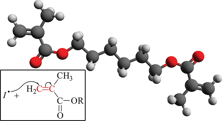
Atomic structure of 1,6-hexanediol dimethacrylate (HDDMA). Hydrogen atoms are in light gray, carbon atoms are in dark gray, and oxygen atoms are in red. The largest distance among atoms of the structure is about 15 Å. The inset shows a sketch of the radical addition mechanism. The radical photoinitiator reacts with one of the two vinyl groups (in red), opening the double bond and shifting the radical site to the most substituted carbon.

Since the viscous and mechanical properties of photocured materials are critically affected by the type of polymer used, understanding the molecular structure and topology of the polymer network as well as its dynamics during polymerization remains essential. A complex polymeric matrix, for example, could hinder chain mobility, shrinkage processes, and location of the gelation point, thus potentially jeopardizing propagation and termination reactions.¹⁶⁻¹⁸ From an experimental standpoint, the topological characterization of the network formation often remains elusive, due to the fast reaction rates and the intricate structure of the polymer mesh.

Hence, computer simulations are a fundamental tool to tackle such problems.¹⁹⁻²³ Although the simulation of the whole process, comprising the interaction between light and the material plus the chemical reactions responsible for the polymer growth, is currently not feasible, precious insights can be gained through an approximate description. In particular, several kinetic modeling approaches and ab initio techniques have been used to probe the network formation process in step-growth polymerization for comprehending the features related to the development of the polymer structures, such as gel point, cross-linking density, and final physical properties of the network, like Young’s modulus, viscosity, and tensile strength²⁴⁻²⁶ On the other hand, over the last 2 decades, classical molecular dynamics (MD) methods have gained much popularity because of their detailed atomistic description granted at reduced computational costs, if compared, for example, with the typical ones needed for purely ab initio techniques. More specifically, a reactive version of the classical MD can describe the formation of the cross-link bond among monomers with number of bonds engaged by a single monomer larger than two (degree), leading to the generation of a polymer.

Reactive MD methods can be built following two alternative procedures. The first one relies on the use of environment parametrized force fields,²⁷⁻³⁰ such as the reactive force field (ReaxFF),³¹ the Empirical Valence Bond,³² and the Adaptive Intermolecular Reactive Empirical Bond Order (AIREBO),³³ successfully employed to model the polymerization in carbon composites and thermal decomposition of polymers.³⁴⁻³⁶ The second one adopts a topological reactive approach³⁷ which essentially consists of an algorithm that, once the specific topology of the prereacted template is matched, adds a new bond, if a set of predetermined conditions (mainly distance cutoffs and probability transition coefficients) is fulfilled,³⁸ propagating the radical site.

This method has been used, for example, to study the mechanical properties of cured epoxy resins, providing a value of Young’s modulus in close agreement with the experimental one.³⁹ It has also been applied to simulate the thermomechanical properties of hexanediol diacrylate (HDDA) polymer networks⁴⁰ and the photoinduced polymerization of diacrylate, at different curing light intensities and photoinitiator concentrations.⁴¹ Further notable examples include the heat conduction in polydisperse polyethylenimine⁴² and poly(3,4-ethylenedioxythiophene),⁴³ as well as the formation of flattened carbon nanotube/polyimide nanocomposites.⁴⁴

In the present work, we use the classical MD alongside with the topological reactive approach to simulate the polymerization of HDDMA and in particular the formation of covalent bonds among monomers. In particular, the HDDMA monomer, having two vinyl groups, could form up to four new covalent bonds. In the following, the number of bonds engaging a monomer defines the degree of the molecule (the maximum possible degree of a HDDMA molecule is four). First, all HDDMA molecules have degree zero (since they are monomers). As polymerization proceeds, the monomers become covalently bonded to other HDDMA molecules providing to molecules with degree one, two and eventually three and four, forming cross-links. The classical MD is found to correctly compute a number of thermodynamic quantities characterizing the initial monomer blend, such as diffusion constant and viscosity and the topological features of the resulting polymer solution. Our reactive MD simulations show, for example, that the number of polymer loops (also termed as cycles) increases during the polymerization, with a maximum size ranging between two and four, although larger structures (up to size 10) also appear. Their formation is generally penalized for a higher initial concentration of monomers, while linear chains are more favored. The concentration of monomers also affects the location of the gel point, which is found to shift toward higher values of rate of double bond conversion, a behavior also observed in HDDA.⁴⁰ Finally, an estimation of Young’s modulus around 4 GPa is also provided.

The paper is organized as follows. In the Computational Details section, we describe the computational approach used to simulate the polymerization of HDDMA, while in the section Results, we discuss the thermodynamic properties of the liquid monomer and the mechanical and topological features of the polymerization as well as the mechanical properties of the initial monomer blend. Some final remarks close the manuscript.

2. Computational Details

2.1. Classical HDDMA Modeling

Classical molecular dynamics (whose equations are integrated using LAMMPS) is used to model both HDDMA monomers and the corresponding polymer.⁴⁵ In this work, we exploit the TraPPE United Atoms (UA) classical force field,⁴⁶⁻⁵¹ a method which implicitly embeds hydrogen atoms in the carbon atomic description, so that each carbon describes a methyl (−CH₃) or a methylidene (=CH₂) group. A list of parameters is reported in Supporting Information. With respect to all-atom force fields (such as OPLS-AA and Amber Force Fields), the TraPPE UA reduces the complexity of the simulations, preserving accurate benchmarks against multiple phases, densities, and temperatures. Although the original formulation implements rigid interatomic bonds, here we adopt elastic bond interaction potentials to simulate the cross-linking bond.

To observe the volume shrinkage effect, the isothermal–isobaric (NPT) ensemble is chosen and simulated through a Nose–Hoower thermostat,⁵²⁻⁵⁶ with a chain length of 3 in pressure and temperature,¹⁰¹, fixed at 1 atm and 400 K respectively.⁵⁷ With this temperature, the system is in a liquid state above the glass transition, thus allowing the reaction to proceed. The relaxing time of the NPT thermostat is set equal to 0.1 and 1.0 ps, respectively, for the temperature and pressure, while the integration time step is fixed at 1 fs.

2.2. Classical Reaction Modeling

The initiation step is modeled introducing a predefined quantity of active monomers reacting with the unreacted ones. The amount of active radicals depends on the kind of initiator, on the characteristics of the light irradiating the material and on the exposure time. The photoactivation can be treated either as a probabilistic event⁵⁸ or by setting an initial fixed number of free radicals, mimicking the effect of a very short intense light beam.^40,58 In this work, we use the second approach. In particular, we randomly extract a set of a given number of vinyl groups among the HDDMA molecules. Then, the selected vinyl groups are modified to radical sites. The ratio between the number of modified vinyl groups and the total number of vinyl groups before the random selection is defined in the following as the initial radical concentration.

The process of double bond conversion (in the following DBC) occurring in the propagation step is simulated using the reactive molecular dynamics, following the topological approach introduced in the literature.³⁷ This strategy allows for the simulation of large system sizes (tens of nanometers), whose dynamics are generally inaccessible to quantum molecular dynamics, due to the high computational costs of ab initio calculations.

In this topological reactive method, the bond/react fix package of LAMMPS is used to match the topology (type, bonds, angles, dihedrals) of pre- and post-templates (i.e., before and after the formation of the cross-linking bond) of reactive atoms.³⁷ More specifically, whenever a reactive carbon is below a prescribed distance from a reactive vinyl group (−CH=CH₂), the algorithm checks whether the topology of the prereacted template matches with the molecular configuration of the reactant. If the identification step is positive, the carbon atoms change type due to the DBC in a single bond, and a new cross-linking bond is added between the carbon and the vinyl group alongside with the propagating radical site. Once the prereacted template is identified, a random number, ranging between zero and one, is extracted and compared with the reaction probability k, computed as

1

where ΔG_A is the activation free energy of the formation of a cross-linking bond, in the following assessed by ab initio calculations (see Section 2.3), A is the pre-exponential acceleration factor, R is the gas constant, and T is the local temperature.⁵⁹

A sketchy view of the propagation step is schematized in Figure 2, where three templates, containing pre and post configurations, are shown (see Supporting Information). Here, the red filled circles represent the two carbons of the vinyl group (−CH=CH₂) of each half monomer, the unfilled circles indicate the radicals, and the black filled circles represent dead atoms that can not endure further reactions. In the top panel a radical carbon (unfilled circle) changes type due to the reaction with a carbon atom of the vinyl group (red filled circle) forming a new cross-linking bond, represented with a headless black line. Note that the HDDMA monomer contains two vinyl group. Once the bond is created, the radical unit is transferred to this half monomer (middle panel of Figure 2), thus realizing the propagation step. Afterward, angles and dihedrals (whose complete list is reported in Supporting Information) are modified as prescribed by the force filed parameters and according to the post reaction template. It is worth noting that a detailed knowledge of the topology is crucial to assess Young’s modulus and the volume shrinkage during the polymerization.

Figure 2.

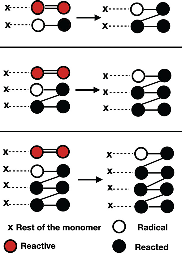
Schematic representation of the three templates used to simulate the propagation reaction mechanism. The red circles represent the potentially reactive carbons of the vinyl group, the white circle represents the radical site, and the black circles represent the reacted ones. The rest of the monomer is represented with a cross. Note that the presence of a second vinyl group in the HDDMA (here represented with the cross) makes possible the formation of cross-links.

Finally, the termination process is modeled by a probabilistic rule in order to describe the ratio between disproportionation and combination reactions whose ratio is significantly high in acrylate compounds.⁶⁰⁻⁶² In particular, a pseudorandom number is extracted from the uniform distribution within the unit interval when two radical atoms are close enough. If the pseudorandom number is lower than a threshold value, the two radicals proceed according to the disproportionation way without forming an extra bond. Otherwise, the combination way is modeled with an additional bond alongside the associated angle and dihedral parameters. The threshold value was set according to the ratio disproportionation/combination 73/27 experimentally measured for the PMMA.⁶¹

2.3. Ab Initio HDDMA Calculations

Ab initio calculations are used to estimate the activation energy needed for the addition of a HDDMA monomer to a radical HDDMA dimer, connected to a tert-butyl group (reproducing the situation due to the action of an azobis(isobutyronitrile)-AIBN radical initiator). Then, the estimated activation energy is corrected for the zero-point energy and for thermal contribution, the last one being evaluated in NWChem for a canonical ensemble of a nonlinear polyatomic ideal gas.⁶³ Finally, the solvation energy was estimated by the conductor-like screening model (COSMO)⁶⁴ in the version provided by York and Karplus⁶⁵ using the modified scaling form of the dielectric constant proposed by Stefanovich and Truong⁶⁶ with the radius parameters for the spherical molecule-shaped cavity suggested by Klamt et al.⁶⁷ The resulting activation free energy ΔG_A is used in eq 1.

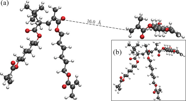
The location of the transition state is obtained using the nudged elastic band (NEB) method,⁶⁸ in which the initial energy path lies between the optimized HDDMA trimer structure (taken as initial configuration of the band) and the structure corresponding to a monomer placed at 16 Å from a HDDMA dimer (final configuration of the band, see Figure 3). The covalent bond of the optimized HDDMA trimer between the carbon atoms of the dimer and the monomer is used to trace the unit vector pointing the direction of the monomer position in the final configuration (with the two carbons involved in the covalent formation placed at 16 Å).

Figure 3.

(a) Optimized structures (dimer and monomer) of HDDMA, with the two carbons forming the covalent bond placed at a distance of 16 Å. In the inset (b), the optimized trimer HDDMA structure is reported.

Theoretical calculations are carried out using the NWChem program of the Environmental Molecular Sciences Laboratory,⁶⁹ based on the density functional theory (DFT) implementation of the exchange-correlation functional B3LYP (Becke three-parameter exchange functional (B3)⁷⁰ and the Lee–Yang–Parr correlation functional (LYP)⁷¹) of the Los Alamos National Laboratory 2-double-z (LanL2DZ) basis sets.⁷² The ultrafine grid is used for energy, gradients, and Hessians.

2.4. Dynamical Approach to Nonequilibrium Molecular Dynamics

To investigate different properties of the polymer (e.g., gel point, Young modulus) we use the dynamical approach to nonequilibrium molecular dynamics (D-NEMD) introduced by Orlandini, Meloni, and Ciccotti.⁷³ The D-NEMD extends a previous method initially introduced by Ciccotti and co-workers,^74,75 where the initial state is determined by a macroscopic condition (e.g., isothermal–isobaric equilibrium). Let us denote Ô(Γ) as a generic observable which is a function of the point in the phase space Γ = (r⃗,p⃗). In a nonequilibrium system the expectation value of this observable, O̅(t), is the ensemble average over the probability density function (PDF) f(Γ, t) at time t given as

2

It is worth to highlight that f(Γ,t) respects the Liouville equation:

3

where {·,·} denotes the Poisson bracket and L(t) is the Liouville operator. Usually, the direct evaluation of the PDF, Γ = (r⃗,p⃗), at time t is extremely difficult to be obtained, apart from simple cases. On the other hand, we can get around the problem by using the Onsager–Kubo relation:

4

where S(t) is the time-evolution operator of the phases space, Γ, and S*(t), its adjoint, represents the time-evolution operator of the PDF. On the other hand, the PDF, f(Γ,t₀), at the initial time, t₀, can be easily sampled, since the system is microscopically determined (e.g., given temperature and pressure). Thus, the eq 4 can be used to compute O̅(t) by an alternative approach. Precisely, we use N trajectories starting from a set of phase space points, {Γ₀ⁱ}_i=1,N, which are distributed over the PDF f(Γ,t₀). At any time t, the time dependent average O̅(t) is assessed as

5

where Ô(Γ(t,Γ₀ⁱ)) denotes the value of the observable, Ô, assumed at time t along the ith trajectory started from the phase space point, Γ₀. Note that in the present work we assume that f(Γ,t₀) is the PDF of a system at constant number of atoms, temperature, and pressure.

3. Results

3.1. Liquid Monomer Properties

To begin, we perform an NPT 10 ns equilibration of 2250 monomers which correspond to 40 500 atoms. The initial length of each axis is set to 200 Å. The last 4 ns of the trajectory is used to estimate the equilibrium volume V = 1.04973(13) × 10⁶ ų and the density ρ = 0.986(2) g/cm³. The experimental value at 300 K is about 0.995 g/cm³, confirming a good agreement with the numerical density value (less than 1%). The diffusion coefficient is obtained by a linear fit of R²(t), through the well-known expression

6

where N is the total number of atoms and represents the position of the ith atom at time t. The resulting value is D = 1.17 × 10^–5 cm²/s, which is in good agreement with the value reported in ref (76) for an hydroxyethyl methacrylate dimer (about 0.98 × 10^–5 cm²/s at 323 K).

To further test the quality of the model, we also calculate the shear viscosity of the monomers using the D-NEMD method⁷⁷⁻⁷⁹ (see Section 2.4). We use the SLLOD method⁸⁰⁻⁸² to simulate a shear flow, with a rate, in the xy plane, of 1.25 × 10¹⁰ s^–1. The shear viscosity can be estimated using the following expression⁸³

7

where is the virial stress tensor estimator in the x, y direction. The numerator is assessed at t = 0 by averaging over a number of initial configurations obtained by sampling an equilibrium NPT ensemble. Then, each configuration evolves independently for a time t under a shear rate γ, giving an estimation of the time-dependent average . Finally, the independent trajectories are run until a plateau in time of is attained.

We use 200 initial trajectories sampled every 20 ps and evolved for 250 ps (see Figure 4). The calculated viscosity is 5.9 ± 0.1 cPs, in good agreement with experimental results in ref (84), where a value of 6 cPs is reported.

Figure 4.

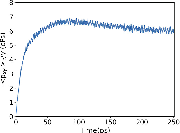
Value of η given in eq 7 averaged over 200 trajectories. The error bars are within the symbols.

3.2. Polymerization Characterization

3.2.1. Activation Energy

To get insights into the formation of the cross-link, we compute the activation free energy ΔG_A (required in eq 1) using the NEB method (see Section 2.3). This is done by considering a set of different images (in our simulations we have 128 images), linearly interpolated between the initial configuration (the optimized trimer) and the final one (the dimer and the monomer placed at distance equal to 16 Å; see also panels a and b of Figure 3), relaxed via ab initio calculations. The process lasts until the energy path matches the minimum energy one in the potential energy surface (PES), within a given tolerance gap in the maximum and root-mean-square gradient values.

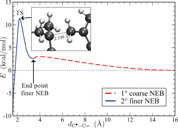
The PES profile along the relaxed path is shown in Figure 5 as a function of the distance between the carbon atoms reacting to form the new covalent bond. Importantly, since a finer mesh size in the NEB improves the accuracy of the transition state (TS) description, a second path of images (whose number has been taken once again equal to 128) is relaxed among the initial state (the trimer) and the relative minimum located at 3.45 Å (see Figure 5).Then, using the potential energy measured at as a zero energy reference, the activation energy corrected for the zero point vibrational energy is estimated equal to ΔE_A = 11.3 kcal/mol, whereas the activation energy corrected by the COSMO model for the solvation correction is equal to ΔE_A = 12.1 kcal/mol. Finally, the activation free energy computed by both solvation and thermal corrections (see Section 2.32.3) at 400 K is ΔG_A = 12.0 kcal/mol.

Figure 5.

Profile of the PES along the minimum energy path (MEP) projected over the distance between the carbon atoms reacting to the covalent bond. The red dashed line represents the MEP obtained by the coarse NEB extended up to 16 Å, while the blue continuous one shows the MEP from the finer NEB, computed up to the local minimum placed at 3.45 Å. Note that the profile of the PES is reported without the COSMO solvation correction. In the inset, two reacting carbons are drawn at the transition state.

Once ΔG_A is computed, one needs to calculate the probability coefficient k of the reaction, which is necessary to perform the identification step in the topological reactive method. Two different strategies are used. In the first one (reaction model A), the superimposed structure is controlled at each time step with the probability coefficient k set equal to 1, while in the second one (reaction model B), it is checked, once again, at each integration step but with k computed from eq 1. In both cases an integration time step of 1 fs is employed. In the model B, since the ΔG_A is assessed via ab initio calculations, the pre-exponential acceleration factor can be interpreted as A = κ[(k_BT)/h] (following the Eyring equation⁸⁵ of the transition state theory), where κ is the transmission coefficient equal or lower than 1, k_B is the Boltzmann constant and h is the Planck constant. Assuming κ = 1, the reaction probability is k ≃ 10^–8 per each time step, making the cross-link formation highly unlikely to occur. If, for example, two monomers are in the configuration to react, such probability would be lower than 2% in 1 ns of simulation. Thus, we conclude that the standard molecular dynamics cannot sample the polymerization events by the simulation time commonly reachable by typical computational facilities (e.g., a few microseconds). In other words, the cross-linking process, adopting the real ΔG_A, is a rare event, so the statistical sampling of the polymerization process is hindered by the free energy barrier. To get around the problem, we set the pre-exponential acceleration factor equal to A = 10 000[(k_BT)/h] to accelerate the cross-link event and observe the polymerization process numerical simulations. This corresponds to a probability of about 30% to observe the cross-link event in one picosecond of simulation. However, in Sections 3.2.4 and 3.2.3, we will show that different acceleration factor values do not bias the main features of the polymer network, such as the gel point and cyclomatic complexity, confirming the validity of the present approach in accelerating the dynamics of the cross-linking formation and, concurrently, preserving the essential features of the final polymer obtained in the simulations.

3.2.2. Double Bond Conversion

We consider three different values of initial radical concentration (in the following RC), equal to 1%, 3% and 5%, at a pressure of 1 atm. Simulations are stopped when approximately 80% of double bonds are converted (see Figure 6). A higher bond conversion is hard to achieve as the mobility of the system slows down dramatically with curing. For instance, the self-diffusion coefficient computed by eq 6 on both the unreacted and reacted HDDMA molecules of the case initial radical concentration 3% as a function of bond conversion shows a clear decrease, equal to 1.17 × 10^–5, 0.38 × 10^–5, 0.16 × 10^–5, and 0.11 × 10^–5 cm²/s for the bond conversion values: 0%, 25%, 50%, and 75%, respectively. Furthermore, the severe self-diffusion limitations provide a drastic decrease in the rate of chain termination steps (also referred to as the Trommsdorff effect⁸⁶), which yields a decrease in the radical concentration always lower than 5% in all simulations.

Figure 6.

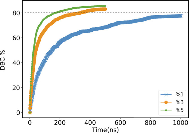
Double bonds conversion (in percentage) for model A as a function of time for different concentrations. Simulations are run until a value of ≃80% of DBC is attained. For model B, the DBC is about 10 times slower.

The cutoff distance for the reaction is fixed at 4 Å and checked at each time step (equal to one femtosecond), in both models A and B. In model A, we observe a higher frequency of DBC, particularly at early time steps and for larger concentration of active monomers. This is the consequence of a reaction probability to form a new bond much smaller than that in model B.

3.2.3. Number of Cycles and Cyclomatic Complexity

Characterizing the topological properties of the polymerization is essential to gain insights about relevant quantities, such as the gel point and Young’s modulus. For example, it has been found that the formation of primary and secondary polymer loops (or cycles) in the polymeric network may lead to a significant shift on the gel point toward lower concentrations of active monomers.⁸⁷⁻⁸⁹ Our simulations suggest that this behavior holds for HDMMA as well. Thus, the present reactive MD approach is combined with the graph theory to extract topological information on the polymer network, contributing to the vast effort afforded in the past decade to quantify the effect of the polymer network’s complexity on the gel point and elasticity.^{24,40,90−92} In particular, we identify these clusters by using methods of the graph theory, where each HDDMA molecule is a node and the bond (connections) between them are edges of a graph. A cluster is defined as a set of connected HDDMA molecules (nodes) where, given any pair of nodes in the same cluster, exists at least one path of connections (edges) linking the two nodes of the pair. Thus, we use the Deep First Search (DFS) method.⁹³ The DFS method is able to identify all the HDDMA molecules belonging to a same cluster, also if they are not directly connected, and the number of such clusters.

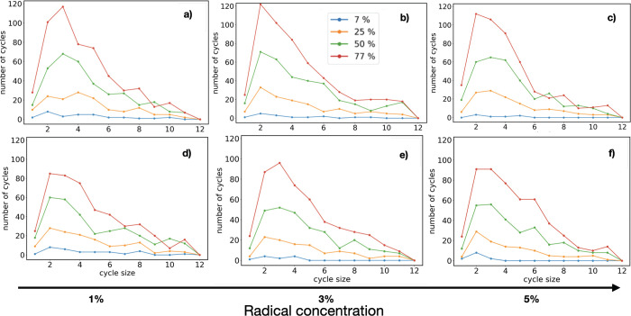
We use the Python library NetworkX⁹⁴ to calculate the number of cycles. Figure 7 shows the number of cycles as a function of the cycle size (defined as the number of indirectly connected monomers in a loop) for different values of DBC and RC. Panels a–c show the results obtained from model A (with the check frequency equal to 1 fs), while the panels d–f show those from model B. At the initial stage of polymerization (DBC around 7%, blue lines), the number of large cycles (i.e., those with more than four monomers) is rather small, and most of the cycles have size equal to 2. For all RC values under consideration, we observe that cycles of size larger than 2 are almost negligible although, as the reaction proceeds (higher DBC) their number generally increases. However, we observe that the total number of cycles at low 1% RC is larger than the total number of cycles for larger concentrations in the initial stage of the polymerization.

Figure 7.

Number of cycles of a given size at different DBC values reported in the legend (7%, 25%, 50%, and 77%) and RC amounts: (a–c) model A; (d–f) model B.

For example, at a DBC of 7% (initial phase of polymerization process), the total number of cycles is 31, 12, and 11 for 1%, 3%, and 5% of RC in reaction model A, and 30, 11, and 12 in reaction model B. Both the models A and B show that the increase in RC disfavors the formation of loops. On the other hand, we observe that the final results are almost independent of the reaction model A and B, used to accelerate the cross-link formation. As the DBC augments, cycles of larger size appear and the plots (yellow, green, and red ones in Figure 7) show a similar behavior, regardless of the RC value.

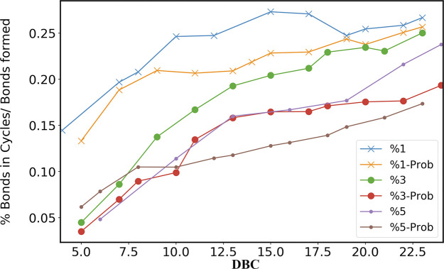
An intriguing question is whether the decrease in the number of loops corresponds to an increase of linear polymer chains at high values of RC. To this purpose, we probe the ratio of the number of formed covalent bonds involved in the formation of cycles to the total number of formed covalent bonds (in both cycle and linear structures) shown in Figure 8 for different concentrations and reaction probabilities. The Figure 8 clearly shows that high values of initial RC suppress the formation of cycles in favor of linear polymer chains, since the largest part of the formed covalent bonds are involved in noncyclic structures. Finally, in the last stage of the polymerization, HDDMA systems exhibit similar topological properties, regardless of the RC values, a behavior also observed, for example, in BPA polymers.⁴¹

Figure 8.

Ratio of the number of bonds involved in the formation of cycles to the total number of bonds vs DBC, for different values of RC. In the legend, the curves labeled only with the initial amount of radicals correspond to the check frequency of 1 fs (model A), while the ones labeled with “Prob” are obtained with the reaction probability given in Section 3.2.1 (model B).

The percentage of cross-linked monomers (i.e., monomers with more than two bonds) and the cyclomatic complexity (indicating the number of elementary cycles not containing further cycles) are also expected to change during the polymerization process. Their behavior is shown in Figure 9, where the cyclomatic complexity is defined as Cyc = B – M + C, with B being the number of bonds, M the number of monomers, and C the number of clusters. They monotonically increase as the reaction proceeds, with negligible differences for RC values.

Figure 9.

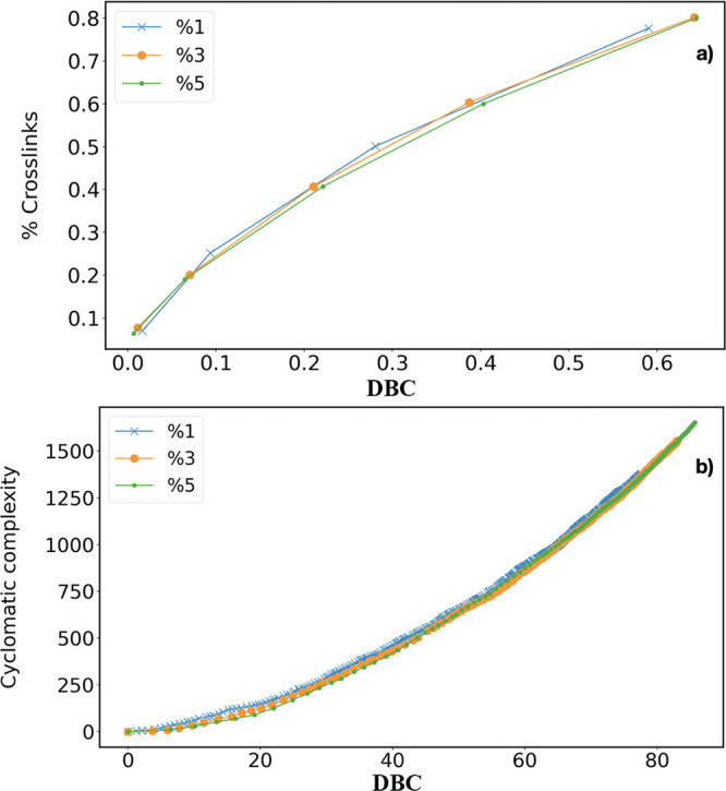
(a) Percentage of cross-linked monomers (monomer with more than two bonds) at different DBC and RC in model A. (b) Cyclomatic complexity at different DBC and RC in model A.

3.2.4. Gel Point

In this section, we probe the effect of different values of RC on the gel point. Characterizing the gel point is fundamental since, at it, the system undergoes a transition from a fluid toward a solid-like behavior, and the viscosity abruptly augments. Following the approach introduced by Torres-Knoop et al.,⁴⁰ the gel point can be identified by monitoring the inflection point of the maximum size of the cluster versus the rate of DBC (Figure 10).

Figure 10.

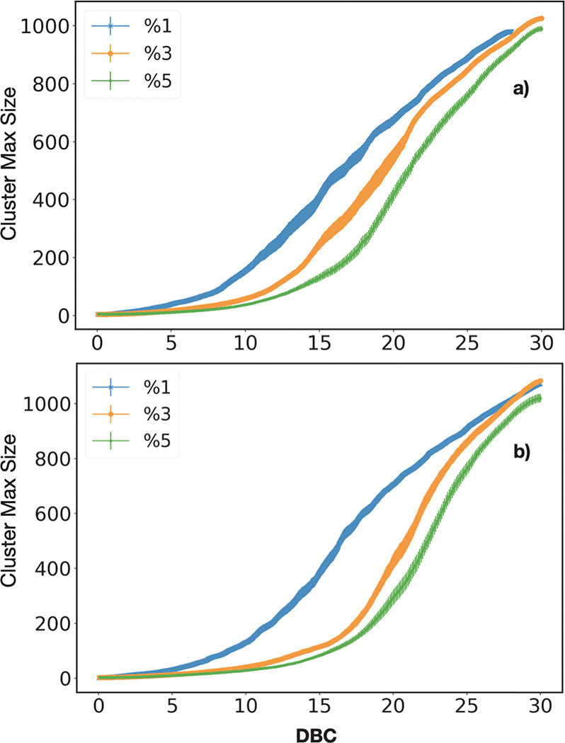
Maximum size of the cluster vs DBC, for three values of RC, in model A (a) and in model B (b), respectively.

Using the following logistic function

8

one has an inflection point located at x_gel = b[(c – 1)/(c + 1)]^1/c, where a, b, c, and d are fitting parameters. This represents the estimate of the rate of DBC at which the gel transition takes place. The linear term in n_max(x) is included to improve the fit without modifying the analytical location of the inflection point x_gel (the variance is calculated as that of the random variable x_gel obtained for the 20 independent curves). Hence, the gel point is obtained by fitting the max size versus DBC curve averaged over 20 independent trajectories within values ranging between 0% to 30% of the DBC. Following the D-NEMD approach⁷⁷⁻⁷⁹ introduced in Section 2.4, the starting configurations for the independent trajectories have been sampled from an isobaric–isothermal simulation of the initial monomer liquid at the equilibrium with 400 K and 1 atm.

We get x_gel ≃ {15.8 ± 0.9, 18.9 ± 0.4, 21.2 ± 0.4} for 1%, 3%, and 5% in reaction model A, and x_gel ≃ {16.2 ± 0.3, 21.2 ± 0.4, 22.6 ± 0.3} for 1%, 3%, and 5% in reaction model B. In both the models A and B, we observe as the high values of RC increase the DBC of the gel point. Furthermore, the different DBC values of the gel point stem from the different quantity of linear structures in the polymer network, whose number increases for larger values of RC. Indeed, since linear clusters have a higher radius of gyration, their mobility is lower than cyclic ones, an effect that limits their rotational degree of freedom providing the shift of the gel point toward higher values of DBC. Note also that gel points are systematically shifted toward higher values of DBC in model B, once again because of the lower number of cycles (thus higher number of linear structures) in the early stage of polymerization (see Figure 8).

Inspecting the topological arrangement of clusters of monomers during the polymerization confirms the previous results. In the top panel of Figure 11, we show the reactive monomers with their connectivity at different rates of DBC (horizontal direction) and RC (vertical direction). At RC equal to 1% (top panel, top row of images in Figure 11), the latter give rise at a unique giant cluster at 16% of DBC, a result in agreement with a gel point located at x_gel ≃ 16. At RC equal to 3% (top panel, middle row of images in Figure 11), clusters of monomers are still present at 16% of DBC, while a large aggregate emerges only at 19%, thus basically confirming that x_gel ≃ 19. Finally at RC 5% (top panel, bottom row in Figure 11), a giant cluster appears around 22% of rate of DBC, whereas for lower values the polymerization exhibits only separated groups of monomers. These results, in agreement with recent studies,^40,95 indicate that the atomistic model used in our simulations provides an accurate description of the microscopic physics of the photopolymerization for both of the reaction models A and B.

Figure 11.

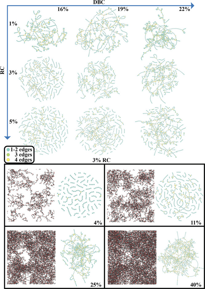
Top panel: Graphical representation of the reacted monomers at different DBC and initial values of RC. Here, the colors indicate the number of connections for each monomer (node of the graph). Bottom panel: The polymerized structure is shown (for the case at RC equal to 3%), at different stages of DBC, indicated in each subpanel.

3.3. Final States Characterization

3.3.1. Volume Shrinkage

The volume shrinkage stems mainly from the formation of the new covalent bonds occurring along the polymerization process. Further, the different packing efficiency in the monomer liquid and the final polymer state provides a relevant change in the free volume of each HDDMA molecule. The volume shrinkage was assessed on the volume difference averaged over a MD simulation of 5 ns of the two systems, the monomer liquid state and the final polymer with DBC equal to 80% at 400 K and initial RC equal to 3%. The resulting volume shrinkage is equal to 19 ± 0.25%. As a reference value, we highlight that for the similar diacrylate HDDA the volume shrinkage was experimentally measured by reflective laser scanning in the work by Ji et al.⁹⁶ at the different temperature of 293 K resulting in 16 ± 0.5%.

Further, to characterize the volume difference of the final state of the polymer as a function of the RC value, we run 2 ns of simulation at 1 atm and 400 K, for each RC, starting from the configurations obtained after reaching the desired DBC (larger than 80%). Then, the equilibrated simulations are analyzed to compute the average volumes. The results show that, as expected, increasing values of RC generally leads to a decrease in the volume (Figure 12), although the effect is mild. The effect stems likely from the higher quantity of linear structures in the systems with higher initial RC.

Figure 12.

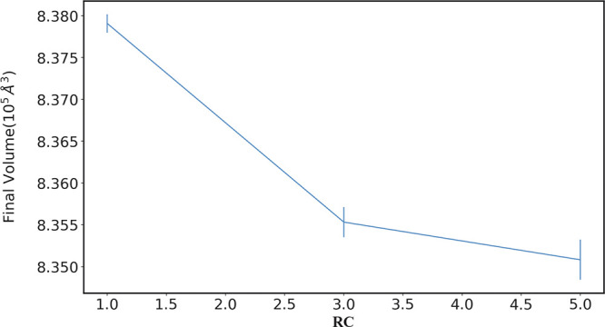
Final volume of the systems equilibrated for 2 ns at 80% of DBC, vs different values of RC.

3.3.2. Young’s Modulus

The elastic properties of the polymerized material can be inspected by monitoring Young’s modulus, computed at 80% of DBC. This is done using the D-NEMD method (see Section 2.4) where the time-dependent average virial tensor is computed during uniaxial extension of the simulation box⁷⁷

9

Here S(t) is the time-evolution operator of an expanding system, whose length has the following time dependence

10

with denoting the strain rate fixed at 10⁹ s^–1. The values of in eq 9 are sampled from an isobaric isothermal simulation of the final polymer at the equilibrium with 400 K and 1 atm, in order to extract independent configuration belonging to the initial phase space, Γ, distribution at time t₀. Also, in the D-NEMD simulations the time-evolution operator S(t) corresponds to the non-Hamiltonian equations of motion of the isothermal–isobaric Nosé–Hoover thermostat,⁵² fixed at 1 atm and 400 K along the y and z directions during the strain deformation, while the side along the x axis follows eq 10. In our work, the virial stress in function of the strain ϵ(t) = (L_x(t) – L₀)/L₀ is averaged over 100 trajectories, each one started from an initial independent configuration.

In panel a) of Figure 13, we show as a function of ϵ(t), for different values of initial RC. In this stress–strain plots, three regimes can be distinguished: (i) the elastic linear regime for strain values raging from 0 to 5%, (ii) the softening regime for strain values going from 5% to 30%, and finally (iii) the hardening regime for higher values of strain rates. Similar curves have been also obtained in experiments and simulations of other polymer systems, such as polybutadiene and polystyrene.^97,98

Figure 13.

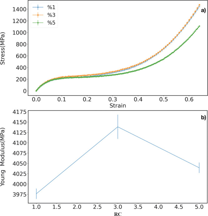
(a) Stress–strain curves for the final polymerized systems starting from different initial values of RC. (b) Young modulus obtained by fitting the linear part of the stress–strain curves for small strain values (0–5%).

Young’s modulus, shown in panel b of Figure 13, can be computed from the angular coefficient of the line fitting the curve within the elastic, linear regime. It is found to range between 3.9 and 4.1 GPa for different values of RC, while experimental values around 3.1 and 4.1 GPa were found for similar systems such as bisGMA and TEGDMA polymers, respectively.⁹⁹

3.3.3. Degree of Heterogeneity

We finally calculate the degree of heterogeneity H for the cured systems as defined in¹⁰⁰

11

where M is the number of monomers, k_min and k_max, respectively the minimum and maximum degree of cross-link bonds (equal to 1 and 4, respectively), and h_het² is a normalization constant.¹⁰⁰H is zero for a network having all monomers with the same number of links (connections) (P(k) is not zero for only one value of k) and has a unity value for a uniform distribution of P(k).¹⁰⁰ In other words, a polymeric network having all the HDMMA molecules bonded to four HDMMA molecules provides the degree of heterogeneity equal to zero. A value of H of about 0.034 was obtained for our systems, indicating very low heterogeneity of the degrees in the final states. In Figure 14 we show the probability P(k) to have a monomer with a given degree k in the polymerized systems, at 80% of DBC. The plots obtained with different RC values exhibit a very similar behavior, except for a small monotonic increase of P(3) and decrease of P(2) for increasing RC. It is worth highlighting that HDDMA molecules of degrees 1 and 3 contain a radical site since the radical reaction shifts a radical site on the molecule. On the other hand, HDDMA molecules of degrees 2 and 4 do not contain a radical site as the second or fourth reaction moves the radical on the adjacent molecule. For the sake of completeness, we also measure the probability that an HDDMA molecule of degree 2 contains at the same time two radical sites which is indeed extremely low (less than 1%). Consequently, the increase in the probability of degrees 1 and 3 for the case 5% of RC stems likely from the larger presence of radical sites, fostering the probability of observing an HDDMA molecule containing a radical site with degrees 1 and 3.

Figure 14.

Probability to have a monomer with a given degree of heterogeneity in the polymerized systems, at 80% of DBC for the three different values of RC.

4. Conclusions

In this work, the reactive classical molecular dynamics has been combined with ab initio calculations and successfully used to study the photopolymerization of the prototypical compound, HDDMA. Also, by the D-NEMD method, our simulations predict the values of many quantities relevant to photopolymers, such as viscosity, gel point, and Young’s modulus, and essential topological features, like chains and polymer cycles observed during curing. The ab initio calculations at the density functional theory level allow for the evaluation of the activation energy necessary to add an HDDMA monomer to a radical HDMMA dimer, showing as the large free energy barrier hinders the probing of the real dynamics in the cross-linking process. Thus, we showed that alternative accelerating strategies (reaction models A and B) could be pursued to provide insights into the process without biasing the features of final polymers.

Furthermore, by varying the concentration of radicals, we monitor the dynamics of linear chains and loops of polymers and find that the latter are generally penalized in systems with a high initial RC of reactive monomers. In this regime, the gel point is found to occur at high values of rate of DBC, i.e., at a relatively late stage of the reaction. On the contrary, gelification is anticipated if the concentration of reactants diminishes. The graph theory was used to analyze the loop formation during the polymerization. In this framework, the topological inspection from modeling studies could also be used to elucidate in future works as the size loop is biased from the rigidity of the monomer segments in the polymeric network. Finally, our model captures the volume shrinkage observed at the final state of the polymerization and, from the stress–strain curve, a value of Young’s modulus of approximately 4 GPa, not far from that found in analogous polymer mixtures.

Supporting Information Available

The Supporting Information is available free of charge at https://pubs.acs.org/doi/10.1021/acs.macromol.1c01408.

• Additional information on the force fields parameters and details of the three templates for the topology reactive algorithm (PDF)

The authors declare no competing financial interest.

References

- Ngo T. D.; Kashani A.; Imbalzano G.; Nguyen K. T.; Hui D. Additive manufacturing (3D printing): A review of materials, methods, applications and challenges. Composites, Part B 2018, 143, 172–196. 10.1016/j.compositesb.2018.02.012. [DOI] [Google Scholar]
- Tumbleston J. R.; Shirvanyants D.; Ermoshkin N.; Janusziewicz R.; Johnson A. R.; Kelly D.; Chen K.; Pinschmidt R.; Rolland J. P.; Ermoshkin A.; et al. Continuous liquid interface production of 3D objects. Science 2015, 347, 1349–1352. 10.1126/science.aaa2397. [DOI] [PubMed] [Google Scholar]
- Zhang J.-Y.; Windall G.; Boyd I. W. UV curing of optical fibre coatings using excimer lamps. Appl. Surf. Sci. 2002, 186, 568–572. 10.1016/S0169-4332(01)00641-9. [DOI] [Google Scholar]
- Rosero-Navarro N.; Pellice S.; Castro Y.; Aparicio M.; Durán A. Improved corrosion resistance of AA2024 alloys through hybrid organic-inorganic sol-gel coatings produced from sols with controlled polymerisation. Surf. Coat. Technol. 2009, 203, 1897–1903. 10.1016/j.surfcoat.2009.01.019. [DOI] [Google Scholar]
- Layani M.; Wang X.; Magdassi S. Novel Materials for 3D Printing by Photopolymerization. Adv. Mater. 2018, 30, 1706344. 10.1002/adma.201706344. [DOI] [PubMed] [Google Scholar]
- Bagheri A.; Jin J. Photopolymerization in 3D Printing. ACS Applied Polymer Materials 2019, 1, 593–611. 10.1021/acsapm.8b00165. [DOI] [Google Scholar]
- Zhou T.; McCarthy E. D.; Soutis C.; Cartmell S. H. Lactone-layered double hydroxide networks: Towards self-assembled bioscaffolds. Appl. Clay Sci. 2018, 153, 246–256. 10.1016/j.clay.2017.11.044. [DOI] [Google Scholar]
- Yu C.; Schimelman J.; Wang P.; Miller K. L.; Ma X.; You S.; Guan J.; Sun B.; Zhu W.; Chen S. Photopolymerizable Biomaterials and Light-Based 3D Printing Strategies for Biomedical Applications. Chem. Rev. 2020, 120, 10695–10743. 10.1021/acs.chemrev.9b00810. [DOI] [PMC free article] [PubMed] [Google Scholar]
- Duval-Terrié C.; Lebrun L. Polymerization and Characterization of PMMA. Polymer Chemistry Laboratory Experiments for Undergraduate Students. J. Chem. Educ. 2006, 83, 443. 10.1021/ed083p443. [DOI] [Google Scholar]
- Ansong O. E.; Jansen S.; Wei Y.; Pomrink G.; Lu H.; Patel A.; Li S. Accelerated controlled radical polymerization of methacrylates. Polym. Int. 2009, 58, 54. 10.1002/pi.2492. [DOI] [Google Scholar]
- Tsarevsky N. V., Sumerlin B. S., Eds. Fundamentals of Controlled/Living Radical Polymerization; Royal Society of Chemistry: 2013; pp 1 – 59. [Google Scholar]
- Clayden J.; Greeves N.; Warren S.. Organic Chemistry; OUP Oxford: 2012. [Google Scholar]
- Tu J.; Makarian K.; Alvarez N. J.; Palmese G. R. Formulation of a Model Resin System for Benchmarking Processing-Property Relationships in High-Performance Photo 3D Printing Applications. Materials 2020, 13, 4109. 10.3390/ma13184109. [DOI] [PMC free article] [PubMed] [Google Scholar]
- Ling L.; Xu X.; Choi G.-Y.; Billodeaux D.; Guo G.; Diwan R. Novel F-releasing composite with improved mechanical properties. J. Dent. Res. 2009, 88, 83–88. 10.1177/0022034508328254. [DOI] [PMC free article] [PubMed] [Google Scholar]
- Anseth K.; Newman S.; Bowman C. Polymeric dental composites: properties and reaction behavior of multimethacrylate dental restorations. Adv. Polym. Sci. 1995, 122, 177–217. 10.1007/3540587888_16. [DOI] [Google Scholar]
- Lang M.; Müller T. Analysis of the gel point of polymer model networks by computer simulations. Macromolecules 2020, 53, 498–512. 10.1021/acs.macromol.9b02217. [DOI] [Google Scholar]
- Gupta A. M.; Hendrickson R. C.; Macosko C. W. Monte Carlo description of A f homopolymerization: Diffusional effects. J. Chem. Phys. 1991, 95, 2097–2108. 10.1063/1.461009. [DOI] [Google Scholar]
- Herrmann H. J. Geometrical cluster growth models and kinetic gelation. Phys. Rep. 1986, 136, 153–224. 10.1016/0370-1573(86)90047-5. [DOI] [Google Scholar]
- De Keer L.; Kilic K. I.; Van Steenberge P. H.; Daelemans L.; Kodura D.; Frisch H.; De Clerck K.; Reyniers M.-F.; Barner-Kowollik C.; Dauskardt R. H.; et al. Computational prediction of the molecular configuration of three-dimensional network polymers. Nat. Mater. 2021, 20, 1422–1430. 10.1038/s41563-021-01040-0. [DOI] [PubMed] [Google Scholar]
- De Keer L.; Van Steenberge P. H.; Reyniers M.-F.; D’hooge D. R. Going Beyond the Carothers, Flory and Stockmayer Equation by Including Cyclization Reactions and Mobility Constraints. Polymers 2021, 13, 2410. 10.3390/polym13152410. [DOI] [PMC free article] [PubMed] [Google Scholar]
- Gartner T. E. III; Jayaraman A. Modeling and simulations of polymers: a roadmap. Macromolecules 2019, 52, 755–786. 10.1021/acs.macromol.8b01836. [DOI] [Google Scholar]
- Karatrantos A.; Clarke N.; Kröger M. Modeling of polymer structure and conformations in polymer nanocomposites from atomistic to mesoscale: A Review. Polym. Rev. 2016, 56, 385–428. 10.1080/15583724.2015.1090450. [DOI] [Google Scholar]
- Glotzer S. C.; Paul W. Molecular and mesoscale simulation methods for polymer materials. Annu. Rev. Mater. Res. 2002, 32, 401–436. 10.1146/annurev.matsci.32.010802.112213. [DOI] [Google Scholar]
- Jin J.; Zheng R.-Q.; Zhou Y.-N.; Luo Z.-H. Network Formation Kinetics of Poly (dimethylsiloxane) Based on Step-Growth Polymerization. Macromolecules 2021, 54, 7678–7689. 10.1021/acs.macromol.1c01131. [DOI] [Google Scholar]
- Desmet G. B.; De Rybel N.; Van Steenberge P. H.; D’hooge D. R.; Reyniers M.-F.; Marin G. B. Ab-Initio-Based Kinetic Modeling to Understand RAFT Exchange: The Case of 2-Cyano-2-Propyl Dodecyl Trithiocarbonate and Styrene. Macromol. Rapid Commun. 2018, 39, 1700403. 10.1002/marc.201700403. [DOI] [PubMed] [Google Scholar]
- Desmet G. B.; Marien Y. W.; Van Steenberge P. H.; D’hooge D. R.; Reyniers M.-F.; Marin G. B. Ab initio based kinetic Monte Carlo analysis to unravel the propagation kinetics in vinyl acetate pulsed laser polymerization. Polym. Chem. 2017, 8, 7143–7150. 10.1039/C7PY01008G. [DOI] [Google Scholar]
- Mueller J. E.; van Duin A. C. T.; Goddard W. A. Application of the ReaxFF Reactive Force Field to Reactive Dynamics of Hydrocarbon Chemisorption and Decomposition. J. Phys. Chem. C 2010, 114, 5675–5685. 10.1021/jp9089003. [DOI] [Google Scholar]
- Yang Y.; Shin Y. K.; Li S.; Bennett T. D.; van Duin A. C. T.; Mauro J. C. Enabling Computational Design of ZIFs Using ReaxFF. J. Phys. Chem. B 2018, 122, 9616–9624. 10.1021/acs.jpcb.8b08094. [DOI] [PubMed] [Google Scholar]
- Schmitt U. W.; Voth G. A. Multistate Empirical Valence Bond Model for Proton Transport in Water. J. Phys. Chem. B 1998, 102, 5547–5551. 10.1021/jp9818131. [DOI] [Google Scholar]
- Marelius J.; Kolmodin K.; Feierberg I.; Aqvist J. Q: a molecular dynamics program for free energy calculations and empirical valence bond simulations in biomolecular systems. J. Mol. Graphics Modell. 1998, 16, 213–225. 10.1016/S1093-3263(98)80006-5. [DOI] [PubMed] [Google Scholar]
- Chenoweth K.; van Duin A. C. T.; Goddard W. A. ReaxFF Reactive Force Field for Molecular Dynamics Simulations of Hydrocarbon Oxidation. J. Phys. Chem. A 2008, 112, 1040–1053. 10.1021/jp709896w. [DOI] [PubMed] [Google Scholar]
- Warshel A.; Weiss R. M. An empirical valence bond approach for comparing reactions in solutions and in enzymes. J. Am. Chem. Soc. 1980, 102, 6218–6226. 10.1021/ja00540a008. [DOI] [Google Scholar]
- Stuart S. J.; Tutein A. B.; Harrison J. A. A reactive potential for hydrocarbons with intermolecular interactions. J. Chem. Phys. 2000, 112, 6472–6486. 10.1063/1.481208. [DOI] [Google Scholar]
- Damirchi B.; Radue M.; Kanhaiya K.; Heinz H.; Odegard G. M.; Van Duin A. C. ReaxFF Reactive Force Field Study of Polymerization of a Polymer Matrix in a Carbon Nanotube-Composite System. J. Phys. Chem. C 2020, 124, 20488–20497. 10.1021/acs.jpcc.0c03509. [DOI] [Google Scholar]
- Odegard G. M.; Jensen B. D.; Gowtham S.; Wu J.; He J.; Zhang Z. Predicting mechanical response of crosslinked epoxy using ReaxFF. Chem. Phys. Lett. 2014, 591, 175–178. 10.1016/j.cplett.2013.11.036. [DOI] [Google Scholar]
- Chenoweth K.; Cheung S.; Van Duin A. C.; Goddard W. A.; Kober E. M. Simulations on the thermal decomposition of a poly (dimethylsiloxane) polymer using the ReaxFF reactive force field. J. Am. Chem. Soc. 2005, 127, 7192–7202. 10.1021/ja050980t. [DOI] [PubMed] [Google Scholar]
- Gissinger J. R.; Jensen B. D.; Wise K. E. Modeling chemical reactions in classical molecular dynamics simulations. Polymer 2017, 128, 211–217. 10.1016/j.polymer.2017.09.038. [DOI] [PMC free article] [PubMed] [Google Scholar]
- Gissinger J. R.; Jensen B. D.; Wise K. E. REACTER: A Heuristic Method for Reactive Molecular Dynamics. Macromolecules 2020, 53, 9953–9961. 10.1021/acs.macromol.0c02012. [DOI] [Google Scholar]
- Okabe T.; Oya Y.; Tanabe K.; Kikugawa G.; Yoshioka K. Molecular dynamics simulation of crosslinked epoxy resins: Curing and mechanical properties. Eur. Polym. J. 2016, 80, 78–88. 10.1016/j.eurpolymj.2016.04.019. [DOI] [Google Scholar]
- Torres-Knoop A.; Kryven I.; Schamboeck V.; Iedema P. D. Modeling the free-radical polymerization of hexanediol diacrylate (HDDA): a molecular dynamics and graph theory approach. Soft Matter 2018, 14, 3404–3414. 10.1039/C8SM00451J. [DOI] [PubMed] [Google Scholar]
- Xie H.; Basu S.; DeMeter E. C. Molecular Dynamics Simulations of Photo-Induced Free Radical Polymerization. J. Chem. Inf. Model. 2020, 60, 6314–6327. 10.1021/acs.jcim.0c01156. [DOI] [PubMed] [Google Scholar]
- Kawagoe Y.; Surblys D.; Matsubara H.; Kikugawa G.; Ohara T. Construction of polydisperse polymer model and investigation of heat conduction: A molecular dynamics study of linear and branched polyethylenimine. Polymer 2019, 180, 121721. 10.1016/j.polymer.2019.121721. [DOI] [Google Scholar]
- Cappai A.; Antidormi A.; Bosin A.; Narducci D.; Colombo L.; Melis C. Impact of synthetic conditions on the anisotropic thermal conductivity of poly (3, 4-ethylenedioxythiophene)(PEDOT): a molecular dynamics investigation. Physical Review Materials 2020, 4, 035401. 10.1103/PhysRevMaterials.4.035401. [DOI] [Google Scholar]
- Patil S. U.; Radue M. S.; Pisani W. A.; Deshpande P.; Xu H.; Al Mahmud H.; Dumitrică T.; Odegard G. M. Interfacial characteristics between flattened CNT stacks and polyimides: A molecular dynamics study. Comput. Mater. Sci. 2020, 185, 109970. 10.1016/j.commatsci.2020.109970. [DOI] [Google Scholar]
- Plimpton S. Fast parallel algorithms for short-range molecular dynamics. J. Comput. Phys. 1995, 117, 1–19. 10.1006/jcph.1995.1039. [DOI] [Google Scholar]
- Martin M. G.; Siepmann J. I. Transferable potentials for phase equilibria. 1. United-atom description of n-alkanes. J. Phys. Chem. B 1998, 102, 2569–2577. 10.1021/jp972543+. [DOI] [Google Scholar]
- Wick C. D.; Martin M. G.; Siepmann J. I. Transferable potentials for phase equilibria. 4. United-atom description of linear and branched alkenes and of alkylbenzenes. J. Phys. Chem. B 2000, 104, 8008–8016. 10.1021/jp001044x. [DOI] [Google Scholar]
- Chen B.; Potoff J. J.; Siepmann J. I. Monte Carlo calculations for alcohols and their mixtures with alkanes. Transferable potentials for phase equilibria. 5. United-atom description of primary, secondary and tertiary alcohols. J. Phys. Chem. B 2001, 105, 3093–3104. 10.1021/jp003882x. [DOI] [Google Scholar]
- Stubbs J. M.; Potoff J. J.; Siepmann J. I. Transferable potentials for phase equilibria. 6. United-atom description for ethers, glycols, ketones and aldehydes. J. Phys. Chem. B 2004, 108, 17596–17605. 10.1021/jp049459w. [DOI] [Google Scholar]
- Kamath G.; Robinson J.; Potoff J. J. Application of TraPPE-UA force field for determination of vapor-liquid equilibria of carboxylate esters. Fluid Phase Equilib. 2006, 240, 46–55. 10.1016/j.fluid.2005.11.034. [DOI] [Google Scholar]
- Maerzke K. A.; Schultz N. E.; Ross R. B.; Siepmann J. I. TraPPE-UA force field for acrylates and Monte Carlo simulations for their mixtures with alkanes and alcohols. J. Phys. Chem. B 2009, 113, 6415–6425. 10.1021/jp810558v. [DOI] [PubMed] [Google Scholar]
- Melchionna S.; Ciccotti G.; Lee Holian B. Hoover NPT dynamics for systems varying in shape and size. Mol. Phys. 1993, 78, 533–544. 10.1080/00268979300100371. [DOI] [Google Scholar]
- Martyna G. J.; Tobias D. J.; Klein M. L. Constant pressure molecular dynamics algorithms. J. Chem. Phys. 1994, 101, 4177–4189. 10.1063/1.467468. [DOI] [Google Scholar]
- Parrinello M.; Rahman A. Polymorphic transitions in single crystals: A new molecular dynamics method. J. Appl. Phys. 1981, 52, 7182–7190. 10.1063/1.328693. [DOI] [Google Scholar]
- Tuckerman M. E.; Alejandre J.; López-Rendón R.; Jochim A. L.; Martyna G. J. A Liouville-operator derived measure-preserving integrator for molecular dynamics simulations in the isothermal–isobaric ensemble. J. Phys. A: Math. Gen. 2006, 39, 5629–5651. 10.1088/0305-4470/39/19/S18. [DOI] [Google Scholar]
- Shinoda W.; Shiga M.; Mikami M. Rapid estimation of elastic constants by molecular dynamics simulation under constant stress. Phys. Rev. B 2004, 69, 134–103. 10.1103/PhysRevB.69.134103. [DOI] [Google Scholar]
- Kollamaram G.; Croker D. M.; Walker G. M.; Goyanes A.; Basit A. W.; Gaisford S. Low temperature fused deposition modeling (FDM) 3D printing of thermolabile drugs. Int. J. Pharm. 2018, 545, 144–152. 10.1016/j.ijpharm.2018.04.055. [DOI] [PubMed] [Google Scholar]
- Okabe T.; Oya Y.; Tanabe K.; Kikugawa G.; Yoshioka K. Molecular dynamics simulation of crosslinked epoxy resins: curing and mechanical properties. Eur. Polym. J. 2016, 80, 78–88. 10.1016/j.eurpolymj.2016.04.019. [DOI] [Google Scholar]
- Ribelli T. G.; Augustine K. F.; Fantin M.; Krys P.; Poli R.; Matyjaszewski K. Disproportionation or combination? The termination of acrylate radicals in ATRP. Macromolecules 2017, 50, 7920–7929. 10.1021/acs.macromol.7b01552. [DOI] [Google Scholar]
- Nakamura Y.; Lee R.; Coote M. L.; Yamago S. Termination mechanism of the radical polymerization of acrylates. Macromol. Rapid Commun. 2016, 37, 506–513. 10.1002/marc.201500677. [DOI] [PubMed] [Google Scholar]
- Nakamura Y.; Yamago S. Termination mechanism in the radical polymerization of methyl methacrylate and styrene determined by the reaction of structurally well-defined polymer end radicals. Macromolecules 2015, 48, 6450–6456. 10.1021/acs.macromol.5b01532. [DOI] [Google Scholar]
- Hill T. L.An introduction to statistical thermodynamics; Courier Corporation: 1986. [Google Scholar]
- Klamt A.; Schüürmann G. COSMO: a new approach to dielectric screening in solvents with explicit expressions for the screening energy and its gradient. J. Chem. Soc., Perkin Trans. 2 1993, 2, 799–805. 10.1039/P29930000799. [DOI] [Google Scholar]
- York D. M.; Karplus M. A smooth solvation potential based on the conductor-like screening model. J. Phys. Chem. A 1999, 103, 11060–11079. 10.1021/jp992097l. [DOI] [Google Scholar]
- Stefanovich E. V.; Truong T. N. Optimized atomic radii for quantum dielectric continuum solvation models. Chem. Phys. Lett. 1995, 244, 65–74. 10.1016/0009-2614(95)00898-E. [DOI] [Google Scholar]
- Klamt A.; Jonas V.; Bürger T.; Lohrenz J. C. Refinement and parametrization of COSMO-RS. J. Phys. Chem. A 1998, 102, 5074–5085. 10.1021/jp980017s. [DOI] [Google Scholar]
- Henkelman G.; Jónsson H. Improved tangent estimate in the nudged elastic band method for finding minimum energy paths and saddle points. J. Chem. Phys. 2000, 113, 9978–9985. 10.1063/1.1323224. [DOI] [Google Scholar]
- Valiev M.; Bylaska E. J.; Govind N.; Kowalski K.; Straatsma T. P.; Van Dam H. J.; Wang D.; Nieplocha J.; Apra E.; Windus T. L.; et al. NWChem: A comprehensive and scalable open-source solution for large scale molecular simulations. Comput. Phys. Commun. 2010, 181, 1477–1489. 10.1016/j.cpc.2010.04.018. [DOI] [Google Scholar]
- Becke A. D. Density-functional thermochemistry. III. The role of exact exchange. J. Chem. Phys. 1993, 98, 5648–5652. 10.1063/1.464913. [DOI] [Google Scholar]
- Lee C.; Yang W.; Parr R. G. Development of the Colle-Salvetti correlation-energy formula into a functional of the electron density. Phys. Rev. B: Condens. Matter Mater. Phys. 1988, 37, 785. 10.1103/PhysRevB.37.785. [DOI] [PubMed] [Google Scholar]
- Pritchard B. P.; Altarawy D.; Didier B.; Gibson T. D.; Windus T. L. New basis set exchange: An open, up-to-date resource for the molecular sciences community. J. Chem. Inf. Model. 2019, 59, 4814–4820. 10.1021/acs.jcim.9b00725. [DOI] [PubMed] [Google Scholar]
- Orlandini S.; Meloni S.; Ciccotti G. Hydrodynamics from statistical mechanics: combined dynamical-NEMD and conditional sampling to relax an interface between two immiscible liquids. Phys. Chem. Chem. Phys. 2011, 13, 13177–13181. 10.1039/c1cp20778d. [DOI] [PubMed] [Google Scholar]
- Ciccotti G.; Jacucci G. Direct computation of dynamical response by molecular dynamics: The mobility of a charged Lennard-Jones particle. Phys. Rev. Lett. 1975, 35, 789. 10.1103/PhysRevLett.35.789. [DOI] [Google Scholar]
- Ciccotti G.; Jacucci G.; McDonald I. Thought-experiments” by molecular dynamics. J. Stat. Phys. 1979, 21, 1–22. 10.1007/BF01011477. [DOI] [Google Scholar]
- Strauch J.; McDonald J.; Chapman B. e.; Kuchel P. W.; Hawkett B. S.; Roberts G. E.; Tonge M. P.; Gilbert R. G. Diffusion Coefficients of the Monomer and Oligomers in Hydroxyethyl Methacrylate. J. Polym. Sci., Part A: Polym. Chem. 2003, 41, 2491–2501. 10.1002/pola.10789. [DOI] [Google Scholar]
- Ciccotti G.; Ferrario M. Dynamical non-equilibrium molecular dynamics. Entropy 2014, 16, 233–257. 10.3390/e16010233. [DOI] [Google Scholar]
- Ryckaert J.-P.; Bellemans A.; Ciccotti G.; Paolini G. Evaluation of transport coefficients of simple fluids by molecular dynamics: comparison of Green–Kubo and nonequilibrium approaches for shear viscosity. Phys. Rev. A: At., Mol., Opt. Phys. 1989, 39, 259. 10.1103/PhysRevA.39.259. [DOI] [PubMed] [Google Scholar]
- Ryckaert J.-P.; Bellemans A.; Ciccotti G.; Paolini G. Shear-rate dependence of the viscosity of simple fluids by nonequilibrium molecular dynamics. Phys. Rev. Lett. 1988, 60, 128. 10.1103/PhysRevLett.60.128. [DOI] [PubMed] [Google Scholar]
- Hoover W. G.; Evans D. J.; Hickman R. B.; Ladd A. J. C.; Ashurst W. T.; Moran B. Lennard-Jones triple-point bulk and shear viscosities. Green–Kubo theory, Hamiltonian mechanics, and nonequilibrium molecular dynamics. Phys. Rev. A: At., Mol., Opt. Phys. 1980, 22, 1690–1697. 10.1103/PhysRevA.22.1690. [DOI] [Google Scholar]
- Evans D. J.; Morriss G. P. Nonlinear-response theory for steady planar Couette flow. Phys. Rev. A: At., Mol., Opt. Phys. 1984, 30, 1528–1530. 10.1103/PhysRevA.30.1528. [DOI] [Google Scholar]
- Daivis P. J.; Todd B. D. A simple, direct derivation and proof of the validity of the SLLOD equations of motion for generalized homogeneous flows. J. Chem. Phys. 2006, 124, 194103. 10.1063/1.2192775. [DOI] [PubMed] [Google Scholar]
- Tuckerman M. E., Ed. Statistical Mechanics: Theory and Molecular Simulation; Oxford University Press: 2010. [Google Scholar]
- Eyring H. The activated complex in chemical reactions. J. Chem. Phys. 1935, 3, 107–115. 10.1063/1.1749604. [DOI] [Google Scholar]
- Tulig T. J.; Tirrell M. Molecular theory of the Trommsdorff effect. Macromolecules 1981, 14, 1501–1511. 10.1021/ma50006a070. [DOI] [Google Scholar]
- Wang J.; Lin T.-S.; Gu Y.; Wang R.; Olsen B. D.; Johnson J. A. Counting secondary loops is required for accurate prediction of end-linked polymer network elasticity. ACS Macro Lett. 2018, 7, 244–249. 10.1021/acsmacrolett.8b00008. [DOI] [PubMed] [Google Scholar]
- Wang R.; Alexander-Katz A.; Johnson J. A.; Olsen B. D. Universal cyclic topology in polymer networks. Phys. Rev. Lett. 2016, 116, 188302. 10.1103/PhysRevLett.116.188302. [DOI] [PubMed] [Google Scholar]
- Zhou H.; Woo J.; Cok A. M.; Wang M.; Olsen B. D.; Johnson J. A. Counting primary loops in polymer gels. Proc. Natl. Acad. Sci. U. S. A. 2012, 109, 19119–19124. 10.1073/pnas.1213169109. [DOI] [PMC free article] [PubMed] [Google Scholar]
- Gu Y.; Zhao J.; Johnson J. A. A (macro) molecular-level understanding of polymer network topology. Trends in Chemistry 2019, 1, 318–334. 10.1016/j.trechm.2019.02.017. [DOI] [Google Scholar]
- Wang R.; Lin T.-S.; Johnson J. A.; Olsen B. D. Kinetic Monte Carlo simulation for quantification of the gel point of polymer networks. ACS Macro Lett. 2017, 6, 1414–1419. 10.1021/acsmacrolett.7b00586. [DOI] [PubMed] [Google Scholar]
- Wang R.; Johnson J. A.; Olsen B. D. Odd–even effect of junction functionality on the topology and elasticity of polymer networks. Macromolecules 2017, 50, 2556–2564. 10.1021/acs.macromol.6b01912. [DOI] [Google Scholar]
- Skiena S. S.The algorithm design manual; Springer: 1998. [Google Scholar]
- https://networkx.org.
- Sarkar S.; Baker P. J.; Chan E. P.; Lin-Gibson S.; Chiang M. Y. Quantifying the sensitivity of the network structure and properties from simultaneous measurements during photopolymerization. Soft Matter 2017, 13, 3975–3983. 10.1039/C7SM00419B. [DOI] [PMC free article] [PubMed] [Google Scholar]
- Ji L.; Chang W.; Cui M.; Nie J. Photopolymerization kinetics and volume shrinkage of 1, 6-hexanediol diacrylate at different temperature. J. Photochem. Photobiol., A 2013, 252, 216–221. 10.1016/j.jphotochem.2012.12.010. [DOI] [Google Scholar]
- Kang Y.; Zhou D.; Wu Q.; Duan F.; Yao R.; Cai K. Fully Atomistic Molecular Dynamics Computation of Physico-Mechanical Properties of PB, PS, and SBS. Nanomaterials 2019, 9, 1088. 10.3390/nano9081088. [DOI] [PMC free article] [PubMed] [Google Scholar]
- Mohammady S. Z.; Mansour A. A.; Stoll B. Dynamic mechanical relaxation behavior of block copolymers at high temperatures. Polymer Physics 2001, 39, 2198–2206. 10.1002/polb.1193. [DOI] [Google Scholar]
- Emami N.; Söderholm K. J. Young’s Modulus and Degree of Conversion of Different Combination of Light-Cure Dental Resins. Open Dent. J. 2009, 3, 202–207. 10.2174/1874210600903010202. [DOI] [PMC free article] [PubMed] [Google Scholar]
- Jacob R.; Harikrishnan K. P.; Misra R.; Ambika G. Measure for degree heterogeneity in complex networks and its application to recurrence network analysis. R. Soc. Open Sci. 2017, 4, 160757. 10.1098/rsos.160757. [DOI] [PMC free article] [PubMed] [Google Scholar]
- The Nosé–Hoover chain thermostat is a generalization of the original Nosé–Hoover algorithm, where a certain number of thermostats are coupled, in chain, to the first one which is, in turn, coupled to the system. The number of thermostats represents the chain length.
Associated Data
This section collects any data citations, data availability statements, or supplementary materials included in this article.