Individualized treatment effects with censored data via fully nonparametric Bayesian accelerated failure time models

Summary

Individuals often respond differently to identical treatments, and characterizing such variability in treatment response is an important aim in the practice of personalized medicine. In this article, we describe a nonparametric accelerated failure time model that can be used to analyze heterogeneous treatment effects (HTE) when patient outcomes are time-to-event. By utilizing Bayesian additive regression trees and a mean-constrained Dirichlet process mixture model, our approach offers a flexible model for the regression function while placing few restrictions on the baseline hazard. Our nonparametric method leads to natural estimates of individual treatment effect and has the flexibility to address many major goals of HTE assessment. Moreover, our method requires little user input in terms of model specification for treatment covariate interactions or for tuning parameter selection. Our procedure shows strong predictive performance while also exhibiting good frequentist properties in terms of parameter coverage and mitigation of spurious findings of HTE. We illustrate the merits of our proposed approach with a detailed analysis of two large clinical trials (N = 6769) for the prevention and treatment of congestive heart failure using an angiotensin-converting enzyme inhibitor. The analysis revealed considerable evidence for the presence of HTE in both trials as demonstrated by substantial estimated variation in treatment effect and by high proportions of patients exhibiting strong evidence of having treatment effects which differ from the overall treatment effect.

1. Introduction

While the main focus of clinical trials is on evaluating the average effect of a particular treatment, assessing heterogeneity in treatment effect (HTE) across key patient sub-populations remains an important task in evaluating the results of clinical studies. Accurate evaluations of HTE that is attributable to variation in baseline patient characteristics offers many potential benefits in terms of informing patient decision-making and in appropriately targeting existing therapies. HTE assessment can encompass a wide range of goals: quantification of overall heterogeneity in treatment response, identification of important patient characteristics related to HTE, estimation of proportion who benefits from the treatment, identification of patient sub-populations deriving most benefit from treatment, detection of cross-over (qualitative) interactions, identifying patients who are harmed by treatment, estimation of individualized treatment effects, optimal treatment allocation for individuals, and predicting treatment effect for a future patient.

Recently, there has been increasing methodology development in the arena of HTE assessment. However, each developed method has usually been targeted to address one specific goal of HTE analysis. For example, Xu and others (2015) and Foster and others (2011) proposed methods to identify patient subgroups whose response to treatment differs substantially from the average treatment effect. Weisberg and Pontes (2015) and Lamont and others (2018) discuss estimation of individualized treatment effects. Zhao and others (2012) discuss construction of optimal individualized treatment rules through minimization of a weighted classification error. Shen and Cai (2016) focus on detection of biomarkers which are predictive of treatment effect heterogeneity. Thus, most existing methods are not sufficiently flexible to address multiple goals of HTE analysis.

The aim of this article is to construct a unified methodology for analyzing and exploring HTE with a particular focus on cases where the responses are time-to-event. The methodology is readily extended to continuous and binary response data. The motivation for investigating such a framework is the recognition that most, if not all, of the above-stated goals of personalized medicine could be directly addressed if a sufficiently rich approximation to the true data generating model for patient outcomes were available. Bayesian nonparametric methods are well-suited to provide this more unified framework for HTE analysis because they place few a priori restrictions on the form of the data-generating model and provide great adaptivity. Bayesian nonparametrics allow construction of flexible models for patient outcomes coupled with probability modeling of all unknown quantities which generates a full posterior distribution over the desired response surface. This allows researchers to directly address a wide range of inferential targets without the need to fit a series of separate models or to employ a series of different procedures. Our methodology has the flexibility to address all of the HTE goals previously highlighted. For example, researchers could quantify overall HTE; identify most important patient characteristics pertaining to HTE; estimate the proportion benefiting from, or harmed by, the treatment; and predict treatment effect for a future patient.

Bayesian additive regression trees (BART) (Chipman and others, 2010) provide a flexible means of modeling patient outcomes without the need for making specific parametric assumptions, specifying a functional form for a regression model, or for using pre-specified patient subgroups. Because it relies on an ensemble of regression trees, BART has the capability to automatically detect non-linearities and covariate interactions. As reported by Hill (2011) in the context of using BART for causal inference, BART has the advantage of exhibiting strong predictive performance in a variety of settings while requiring little user input in terms of selecting tuning parameters. Crucially, using BART for HTE analysis also allows the user to avoid the need to pre-specify patient subgroups or to specify a potentially large number of treatment-covariate interaction terms. While tree-based methods have been employed in the context of personalized medicine and subgroup identification by a variety of investigators including, for example, Su and others (2009), Loh and others (2015), and Foster and others (2011), BART offers several advantages for the analysis of HTE. In contrast to many other tree-based procedures that use a more algorithmic approach, BART is model-based and utilizes a full likelihood function and corresponding prior over the tree-related parameters. Because of this, BART automatically generates measures of posterior uncertainty; on the other hand, reporting uncertainty intervals is often quite challenging for other frequentist tree-based procedures though there has been interesting recent work on constructing confidence intervals for random forests (Wager and others, 2014; Wager and Athey, 2015). In addition, because inference with BART relies on posterior sampling, analysis of HTE on alternative treatment scales can be done directly by simply transforming the desired parameters in posterior sampling. Moreover, any quantity of interest for individualized decisions or HTE evaluation can be readily accommodated by the Bayesian framework. In this article, we aim to utilize and incorporate these advantages of BART into our approach for analyzing HTE with censored data.

Accelerated failure time (AFT) models (Wei, 1992) represent an alternative to Cox-proportional hazards models in the analysis of time-to-event data. AFT models have a number of features which make them appealing in the context of personalized medicine and investigating the comparative effectiveness of different treatments. Because they involve a regression with log-failure times as the response variable, AFT models provide a direct interpretation of the relationship between patient covariates and failure times. Moreover, treatment effects may be defined directly in terms of the underlying failure times for the two different treatments.

Bayesian semi-parametric approaches to the accelerated failure time model have been investigated by a number of authors including Komárek and Lesaffre (2007), Johnson and Christensen (1988), Kuo and Mallick (1997), Hanson and Johnson (2002), and Hanson (2006). Kuo and Mallick (1997) assume a parametric model for the regression function and suggest either modeling the distribution of the residual term or of the exponential of the residual term via a Dirichlet process (DP) mixture model, while Hanson (2006) proposed modeling the residual distribution with a DP mixture of Gamma densities. Our approach for modeling the residual distribution resembles that of Kuo and Mallick (1997). Similar to these approaches, we model the residual distribution as a location-mixture of Gaussian densities, and by utilizing constrained DPs, we constrain the mean of the residual distribution to be zero, thereby clarifying the interpretation of the regression function.

Extensions of the original BART procedure to handle time-to-event outcomes have been proposed and investigated by Bonato and others (2011) and Sparapani and others (2016). In Bonato and others (2011), the authors introduce several sum-of-trees models and examine their use in utilizing gene expression measurements for survival prediction. Among the survival models proposed by Bonato and others (2011) is an AFT model with a sum-of-trees regression function and a normally distributed residual term. Sparapani and others (2016) introduce a nonparametric approach that employs BART to directly model the individual-specific probabilities of an event occurring at the observed event and censoring times. To harness the advantages of both BART and AFT models for HTE analysis, we propose a nonparametric version of the AFT model which combines a sum-of-trees model for the regression function with a DP mixture model for the residual distribution. Such an approach has the advantage of providing great flexibility while generating interpretable measures of covariate-specific treatment effects thus facilitating the analysis of HTE.

This article is organized as follows. In Section 2, we describe the general structure of our nonparametric, tree-based AFT model, discuss its use in estimating individualized treatment effects, detail new choices for the BART hyperparameters, and describe our approach for posterior computation. Section 3 examines key inferential targets in the analysis of HTE and describes how the nonparametric AFT model may be utilized to estimate these targets. Moreover, in this section, we demonstrate the use of our nonparametric AFT method to investigate HTE in two large clinical trials involving the use of an ACE inhibitor. In Section 4, we detail the results of two simulation studies that evaluate our procedure in terms of individualized treatment effect estimation, coverage, and treatment assignment. We conclude in Section 5 with a short discussion.

2. Methods

2.1. Notation and nonparametric AFT model

We assume that study participants have been randomized to one of two treatments, which we denote by either or . We let denote a vector of baseline covariates and let denote patient failure time. Given censoring time , we observe 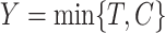and a failure indicator 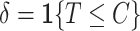We assume also that censoring is noninformative, that is, and are independent given . The data consist of independent measurements . Although, we assume randomized treatment assignment here, our approach may certainly be applied in observational settings. In such settings, however, one should ensure that appropriate unconfoundedness assumptions (e.g. Hill, 2011) are reasonable, so that the individualized treatment effects defined in (2.2) correspond to an expected difference in potential outcomes under the two treatments.

The conventional AFT model assumes that log-failure times are linearly related to patient covariates. We consider here a nonparametric analogue of the AFT model in which the failure time is related to the covariates and treatment assignment through

(2.1)

and where the distribution of the residual term is assumed to satisfy 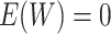. With the mean-zero constraint on the residual distribution, the regression function has a direct interpretation as the expected log-failure time given treatment assignment and baseline covariates.

The AFT model (2.1) leads to a natural, directly interpretable definition of the individualized treatment effect (ITE), namely, the difference in expected log-failure in treatment versus . Specifically, we define the ITE for a patient with covariate vector as

(2.2)

The distribution of in the accelerated failure time model (2.1) is characterized by both the regression function and the distribution of the residual term. In the following, we outline a model for the regression function that utilizes additive regression trees, and we describe a flexible nonparametric mixture model for the residual distribution .

2.2. Overview of BART

BART is an ensemble method in which the regression function is represented as the sum of individual regression trees. The BART model for the regression function relies on a collection of binary trees 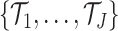and an associated set of terminal node values for each binary tree . Each tree consists of a sequence of decision rules through which any covariate vector can be assigned to one terminal node of by following the decision rules prescribed at each of the interior nodes. In other words, each binary tree generates a partition of the predictor space where each element 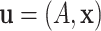of the predictor space belongs to exactly one of the terminal nodes of . The decision rules at the interior nodes of are of the form vs. , where denotes the element of . A covariate that corresponds to the terminal node of is assigned the value and is used to denote the function returning whenever is assigned to the terminal node of .

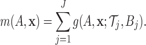
The regression function is represented in BART as a sum of the individual tree contributions

(2.3)

Trees and node values can be thought of as model parameters. The prior distribution on these parameters induces a prior on and hence induces a prior on the regression function via (2.3). To complete the description of the prior on , one needs to specify the following: (i) the distribution on the choice of splitting variable at each internal node; (ii) the distribution of the splitting value used at each internal node; (iii) the probability that a node at a given node-depth splits, which is assumed to be equal to 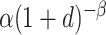; and (iv) the distribution of the terminal node values which is assumed to be . In order to ensure that the prior variance for induces a prior on the regression function that assigns high probability to the observed range of the data, Chipman and others (2010) center and scale the response so that the minimum and maximum values of the transformed response are and respectively. Regarding (i), at each interior node, the splitting variable is chosen uniformly from the set of available splitting variables. Regarding (ii), Chipman and others (2010) suggest a uniform prior on the discrete set of available splitting values though alternative prior distributions for the splitting value are implemented in the R package BayesTree. We discuss our choice for the prior distribution on the splitting values in more detail in Section 2.4.

To denote the distribution on the regression function induced by the prior distribution on with parameter values and total trees, we use the notation . Choices for the hyperparameters 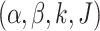are described in more detail in Section 2.4.

2.3. Centered DP mixture prior

We model the density of as a location-mixture of Gaussian densities with common scale parameter . Letting denote the distribution of the locations, we assume the density of (conditional on and can be expressed as

(2.4)

where is the standard normal density function. The DP is a widely used choice for a nonparametric prior on an unknown probability distribution, and when placing a DP prior on G, the resulting DP mixture model for the distribution of provides a flexible prior for the residual density. Indeed, a DP mixture model similar to (2.4) was used by Kuo and Mallick (1997) as a prior for a smooth residual distribution in a semi-parametric accelerated failure time model. The Gaussian location-mixture model in (2.4) is also similar to the flexible approach described in Komárek and others (2005) for modeling the residual distribution in an AFT setting.

Because of the zero-mean constraint on the residual distribution, the DP is not an appropriate choice for a prior on . A direct approach proposed by Yang and others (2010) addresses the problem of placing mean and variance constraints on an unknown probability measure by utilizing a parameter-expanded version of the DP which the authors refer to as the centered DP (CDP). As formulated by Yang and others (2010), the CDP with mass parameter and base measure has the following stick-breaking representation

where and where denotes a distribution consisting only of a point mass at . We denote that a random measure follows a CDP with the notation . From the above representation of the CDP, it is clear that the mixture model (2.4) for and the assumption that together imply the mean-zero constraint, since the expectation of may be expressed as

which equals zero almost surely.

For the scale parameter of , we assume that 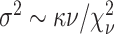, with the default degrees of freedom set to . Instead of specifying a particular value for the mass parameter, we allow for learning about this parameter by assuming where and refer to the shape and rate parameters of the Gamma distribution, respectively.

Our nonparametric model that combines the BART model for the regression function and DP mixture model for the residual density can now be expressed hierarchically as

$$\begin{array}{c}\log T_i=m(A_i,{\mathbf{x}}_i)+W_i,W_i|{\tau }_i,{\sigma }^2\sim N({\tau }_i,{\sigma }^2),\text{ for }i=1,\dots ,n\\ m\sim \text{BART}(\alpha ,\beta ,k,J),{\tau }_i|G\sim G,G|M\sim \text{CDP}(M,G_0)\\ {\sigma }^2\sim \kappa \nu /{\chi }_{\nu }^2,M\sim \text{Gamma}({\psi }_1,{\psi }_2).\end{array}$$ (2.5)

In our implementation, the base measure is assumed to be Gaussian with mean zero and variance . Choosing to be conjugate to the Normal distribution simplifies posterior computation considerably, but other choices of could be considered. For example, a t-distributed base measure could be implemented by introducing an additional latent scale parameter.

2.4. Prior specification

2.4.1. Prior for trees.

For the hyperparameters of the trees , we defer to the defaults suggested in Chipman and others (2010); namely, , , and . These default settings seem to work quite well in practice, and in part F of the supplementary material available at Biostatistics online, we investigate the impact of varying through cross-validation estimates of prediction performance. Our choice for the prior distribution of the splitting value is uniform over the covariate quantiles which is is based on the implementation in the BayesTree package (Chipman and McCulloch, 2016). Further details are provided in part D of the supplementary material available at Biostatistics online.

2.4.2. Prior for terminal node parameters.

As discussed in Section 2.2, the original description of BART in Chipman and others (2010) employs a transformation of the response variable and sets the hyperparameter to so that the regression function is assigned substantial prior probability to the observed range of the response. Because our responses are right-censored, we propose an alternative approach to transforming the responses and to setting the prior variance of the terminal node parameters. Our suggested approach is to first fit a parametric AFT model that only has an intercept in the model and that assumes log-normal residuals. This produces estimates of the intercept and the residual scale which allows us to define transformed “centered” responses . Turning to the prior variance of the terminal node parameters , we assign the terminal node values the prior distribution , where 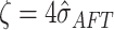. This prior on induces a prior on the regression function and hence assigns approximately prior probability to the interval . Thus, the default setting of assigns prior probability to the interval . Note that assigning most of the prior probability to the interval is sensible because this corresponds to the regression function for the “centered” responses rather than the original responses.

2.4.3. Residual distribution prior.

Under the assumed prior for the mass parameter, we have and . We set and so that the resulting prior on is relatively diffuse with , .

When setting the defaults for the remaining hyperparameters and , we adopt a similar strategy to that used by Chipman and others (2010) for BART when calibrating the prior for the residual variance. There, they rely on a preliminary, rough overestimate of the residual variance parameter and define the prior for in such a way that there is prior probability that is greater than the rough estimate . Here, may be regarded as an additional hyperparameter with the value of determining how conservative the prior of is relative to the initial estimate of the residual variance. Chipman and others (2010) suggest using as the default whenever is set to .

Similar to the approach described above, we begin with a rough over-estimate of the variance of to calibrate our choices of and . A direct way of generating the estimate is to fit a parametric AFT model with log-normal residuals and use the resulting estimate of the residual variance, but other estimates could potentially be used. To connect the estimate with the hyperparameters and described in (2.5), it is helpful to first note that the conditional variance of the residual term can be expressed as

(2.6)

Our aim then is to select and so that the induced prior on the variance of assigns approximately probability to the event 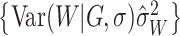, where is treated here as a fixed quantity. As an approximation to the distribution of (2.6), we use the approximation that 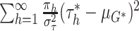has a distribution (see part E of the supplementary material available at Biostatistics online for further details about this approximation). Assuming further that , we have that the variance of is approximately distributed as where , and with this approximation, we can directly find a value of such that . In contrast to the setting suggested in Chipman and others (2010), we set the default to .

With the normal approximation to 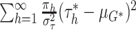, the prior for 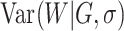has a mean of where is the variance of conditional on a known location and is the variance of the locations. Thus, when , our default setting of means that roughly three-fourths of the prior variation in is attributable to the variance of conditional on location. Rather than fixing , one could introduce an additional hyperparameter that represents the proportion of variation in that is due to variation conditional on location, but we have chosen to fix in order to keep the number of model hyperparameters manageable.

2.5. Posterior computation

The original Metropolis-within-Gibbs sampler proposed in Chipman and others (2010) works by sequentially updating each tree while holding all other trees fixed. As a result, each iteration of the Gibbs sampler consists of steps where the first steps involve updating either one of the trees or terminal node parameters and the last step involves updating the residual variance parameter. The Metropolis-Hastings algorithm used to update the individual trees is discussed in Chipman and others (1998). Our strategy for posterior computation is a direct extension of the original Gibbs sampler, viz., after updating trees and terminal node parameters, we update the parameters related to the residual distribution. In addition, censored values are handled through a data augmentation approach where unobserved survival times are imputed in each Gibbs iteration.

To sample from the posterior of the CDP, we adopt the blocked Gibbs sampling approach described in Ishwaran and James (2001). In this approach, the mixing distribution is truncated so that it only has a large, finite number of components which is done by assuming that, for and . This modification of the stick-breaking weights ensures that 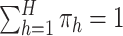. One advantage of using the truncation approximation is that it makes posterior inferences regarding straightforward. Additionally, when truncating the stick-breaking distribution, using the CDP prior as opposed to a DP prior does not present any additional challenges for posterior computation because the unconstrained parameters in (2.5) may be updated as described in Ishwaran and James (2001) with the parameters of interest then being updated through the simple transformation 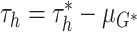. The upper bound on the number of components should be chosen to be relatively large (as a default, we set ), and in the Gibbs sampler, the maximum index of the occupied clusters should be monitored. If a maximum index equal to occurs frequently in posterior sampling, should be increased. A detailed description of our Metropolis-within-Gibbs sampler used for posterior computation is given in part A of the supplementary material available at Biostatistics online. It is worth mentioning that in our implementation, we assume that there is no missing data. A number of missing-data models for the covariates could potentially be directly incorporated into our posterior sampling scheme. In part H of the supplementary material available at Biostatistics online, we describe two particular missing-data models for the covariates, and we discuss how they would be into integrated into our nonparametric AFT model.

3. Posterior Inferences for the Analysis of Heterogeneous Treatment Effects with an Application to Two Large Clinical Trials

The nonparametric AFT model (2.5) generates a full posterior over the entire regression function and the residual distribution. As such, this model has the flexibility to address a variety of questions related to heterogeneity of treatment effect. In particular, we focus in this section on the use of the nonparametric AFT model to answer the following key HTE questions: overall variation in response to treatment, individual-specific treatment effects, evidence for the presence of HTE, and the proportion of patients likely to benefit from treatment. We use two large clinical trials (the SOLVD trials) to illustrate the use of the BART-based nonparametric AFT model in addressing these HTE inferential targets. Applications of the nonparametric AFT model to answer other HTE questions of interest from the SOLVD trial are described in part B of the supplementary material available at Biostatistics online.

The Studies of Left Ventricular Dysfunction (SOLVD) were devised to investigate the efficacy of the angiotensin-converting enzyme (ACE) inhibitor enalapril in a target population with low left-ventricular ejection fractions. The SOLVD treatment trial (SOLVD-T) enrolled patients determined to have a history of overt congestive heart failure, and the SOLVD prevention trial (SOLVD-P) enrolled patients without overt congestive heart failure. In total, patients were enrolled in the treatment trial while patients were enrolled in the prevention trial. The survival endpoint that we examine in our analysis is time until death or hospitalization where time is reported in days from enrollment.

In our analysis of the SOLVD-T and SOLVD-P trials, we included patient covariates common to both trials, in addition to using treatment and study indicators as covariates. These patient covariates contained information from key patient characteristics recorded at baseline (e.g. age, sex, weight, ejection fraction, blood pressure, sodium level, and diabetic status) along with information about patient history (e.g. history of myocardial infarction, history of stroke, smoking history). In our analysis, we dropped those patients who had one or more missing covariates, which resulted in patients being dropped from the total of enrolled in either trial. Currently, our software does not support an analysis where the design matrix contains missing values. However, a number of missing-data models could be directly incorporated into our Gibbs sampling scheme though the computational efficiency of any such scheme will of course depend on specific model details and the size of the dataset to be analyzed. In the supplementary material available at Biostatistics online, we discuss several potential missing-data models and how they could be incorporated into our posterior computation scheme.

3.1. Individualized Treatment Effects

As discussed in Section 2.1, a natural definition of the individual treatment effects in the context of an AFT model is the difference in expected log-survival . Draws from the posterior distribution of allow one to compute fully nonparametric estimates of the treatment effects along with corresponding credible intervals. As is natural with an AFT model, the treatment difference in (2.2) is examined on the scale of log-survival time, but other, more interpretable scales on which to report treatment effects could be easily computed. For example, ratios in expected survival times defined by

(3.1)

could be estimated via posterior output. Likewise, one could estimate differences in expected failure time by using both posterior draws of and of the residual distribution. Posterior information regarding treatment effects may be used to stratify patients into different groups based on anticipated treatment benefit. Stratification could be done using the posterior mean, the posterior probability of treatment benefit, or some other relevant measure.

Figure 1 shows point estimates of the ITEs for patients in both the SOLVD-T and SOLVD-P trials. While the plot in Figure 1 indicates a clear, overall benefit from the treatment, the variation in the ITEs suggests substantial heterogeneity in response to treatment. In the following subsection, we further investigate the evidence for the presence of HTE in the SOLVD trials.

Fig. 1.

Posterior means of with corresponding credible intervals for patients in the SOLVD-T and SOLVD-P trials.

3.2. Assessing Evidence for Heterogeneity of Treatment Effect

As a way of detecting the presence of HTE, we utilize the posterior probabilities of differential treatment effect

(3.2)

along with the closely related quantity

(3.3)

where, in (3.2), is the conditional average treatment effect. Note that is a model parameter that represents the average value of the individual and does not represent a posterior mean. The posterior probability is a measure of the evidence that the ITE is greater or equal to , and thus we should expect both high and low values of in settings where substantial HTE is present. Note that approaches as the value of approaches either or , and whenever . For a given individual , we consider there to be strong evidence of a differential treatment effect if (equivalently, if 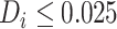or 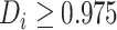), and we define an individual as having mild evidence of a differential treatment effect provided that (equivalently, if or ). For cases with no HTE present, the proportion of patients exhibiting strong evidence of differential treatment effect should, ideally, be zero or quite close to zero. For this reason, the proportion of patients with can potentially be a useful summary measure for detecting the presence of HTE. In this article, we do not explore explicit choices of a threshold for this proportion, but we examine, through a simulation study in Section 4.2, the value of this proportion for scenarios where no HTE is present. It is worth mentioning that the quantity represents evidence that the treatment effect for patient differs from the overall treatment effect, and by itself, is not a robust indicator of HTE across patients in the trial. Rather, the proportion of patients with high values of is what we use to assess evidence for HTE.

It is worth noting that the presence or absence of HTE depends on the treatment effect scale, and is designed for cases, such as the AFT model, where HTE is difference in expected log-failure time. For example, it is possible to have heterogeneity on the log-hazard ratio scale while having no heterogeneity in the ITEs across patients.

Examining the posterior probabilities of differential treatment effect offers further evidence for the presence of meaningful HTE in the SOLVD trials. Table 1 shows that, in the SOLVD-T trial, approximately of patients had strong evidence of a differential treatment effect (i.e. ), and approximately of patients had mild evidence (i.e. ). In the SOLVD-P trial, approximately of patients had strong evidence of a differential treatment effect while approximately had mild evidence. Comparison of these percentages with the results from the simulations of Section 4.2 suggests the presence of HTE. In the null simulation scenarios of Section 4.2, the proportion of cases with strong evidence of differential treatment was very close to zero. Thus, the large proportion of patients with strong evidence for differential treatment effect is an indication that there is HTE in the SOLVD trials that deserves further exploration.

Table 1.

Tabulation of posterior probabilities of treatment benefit and posterior probabilities of differential treatment effect for patients in the SOLVD trials

	SOLVD Treatment Trial	SOLVD Prevention Trial
	51.38	20.47
	24.69	23.71
	20.08	41.98
	3.85	13.84
	0.00	0.00
	19.36	7.30
	41.93	31.58

For each trial, the empirical percentage of patients whose estimated posterior probability of treatment benefit lies within each of the intervals , and is reported. In addition, the percentages of patients in each trial that exhibit “strong” (i.e. ) and “mild” (i.e. ) evidence of differential treatment effect are shown.

3.3. Characterizing heterogeneity of treatment effect

Variability in treatment effect across patients in the study is a prime target of interest when evaluating the extent of HTE from the results of a clinical trial. Assessments of HTE can be used to evaluate consistency of response to treatment across patient sub-populations or to assess whether or not there are patient subgroups that appear to respond especially strongly to treatment. In more conventional subgroup analyses (e.g. Jones and others, 2011), HTE is frequently reported in terms of the posterior variation in treatment effect across patient subgroups. While the variance of treatment effect is a useful measure, especially in the context of subgroup analysis, we can provide a more detailed view of HTE by examining the full distribution of the individualized treatment effects defined by (2.2) where the distribution may be captured by the latent empirical distribution function . Such an approach to examining the “distribution” of a large collection of parameters has been explored in Louis and Shen (1999). The distribution function may be regarded as a model parameter that may be directly estimated by

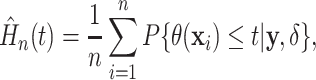(3.4)

and credible bands for may be obtained from posterior samples. For improved visualization of the spread of treatment effects, it is often better to display a density function associated with (3.4) which could be obtained through direct differentiation of (3.4). Alternatively, a smooth estimate can be found by computing the posterior mean of a kernel function with bandwidth

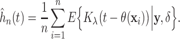(3.5)

The posterior of provides a direct assessment of the variation in the underlying treatment effects, and as such, serves as a useful overall evaluation of HTE.

Figure 2 displays a histogram of the posterior means of the treatment ratios (see eq. (3.1)), for each patient in the SOLVD-T and SOLVD-P trials. In contrast to the ITE scale used in Figure 1, defining the ITEs in terms of the ratios of expected failure times may provide a more interpretable scale by which to describe HTE. As may be inferred from the histogram in Figure 2, nearly all patients have a positive estimated treatment effect with having an estimated value of greater than one. Of those in the SOLVD-T trial, all the patients ha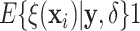d , and of patients in the SOLVD-P trial had .

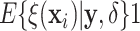Fig. 2.

Histogram of point estimates (i.e. posterior means) of the treatment effects 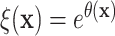and smooth posterior estimates of the treatment effect distribution. The histogram is constructed using all point estimates from both the SOLVD treatment and prevention trials. Smooth estimates, , of the distribution of treatment effects were computed as described in equation (3.5) for the two trials separately. The kernel bandwidth for each trial was chosen using the rule , where and are posterior means of the standard deviation and inter-quartile range of respectively and where is the trial-specific sample size.

Figure 2 also reports the smoothed estimate of the distribution of the treatment effects separately for the two trials. These smoothed posterior estimates of the treatment effect distribution were computed as described in equation (3.5) where posterior samples of were used in place of . Note that the shown in Figure 2 are estimates of the distribution of the underlying treatment effects and do not represent the posterior distribution of the overall treatment effects within each trial. As expected, the variation in treatment effect suggested by the plots of in Figure 2 is greater than the variation exhibited by the posterior means of . The estimates provide informative characterizations of the distribution of treatment effects in each trial especially for visualizing the variability in treatment effects in each trial.

3.4. Proportion who benefits

Another quantity of interest related to HTE is the proportion of patients who benefit from treatment. Such a measure has a direct interpretation and is also a useful quantity for assessing the presence of cross-over or qualitative interactions, namely, cases where the effect of treatment has the opposite sign as the overall average treatment effect. That is, for situations where an overall treatment benefit has been determined, a low- estimated proportion of patients benefiting may be an indication of the existence of cross-over interactions.

Using the treatment differences , the proportion who benefit may be defined as

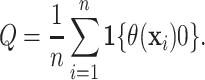(3.6)

Alternatively, one could define the proportion benefiting relative to a clinically relevant threshold , i.e. . The posterior mean of is an average of the posterior probabilities of treatment benefit . Posterior probabilities of treatment benefit can be used for treatment assignment ( vs. ), or as an additional summary measure of HTE where one, for example, could tabulate the proportion very likely to benefit from treatment or the proportion likely to benefit from treatment .

When using (3.6) to estimate the proportion of patients benefiting in each of the SOLVD trials, the estimated proportions of patients (i.e. the posterior mean of in (3.6)) benefiting were and in the SOLVD-T and SOLVD-P trials, respectively. These proportions are approximately equal to the area under the curve of for in Figure 2.

Table 1 shows a tabulation of patients according to evidence of treatment benefit. In both trials, all patients have at least a posterior probability of treatment benefit (i.e. ). In the treatment trial, percent of patients exhibit a posterior probability of benefit greater than , and the corresponding percentage for the prevention trial is .

3.5. Partial dependence and exploring important variables for HTE

To explore patient attributes important in driving differences in treatment effect, we use a direct approach similar to the “Virtual Twins” method used by Foster and others (2011) in the context of subgroup identification. In Foster and others (2011), the authors suggest a two-stage procedure where one first estimates treatment difference for each individual and then, using these estimated differences as a new response variable, one estimates a regression model in order to identify a region of the covariate space where there is an enhanced treatment effect. Similar to this, to examine important HTE variables in the SOLVD trials, we first fit the full nonparametric AFT model to generate posterior means of the individualized treatment effect for each patient. Then, we fit a (weighted) linear regression using the previously estimated as the response variable and the patient covariates (except for treatment assignment) as the predictors. Because the treatment difference should only depend on covariates that are predictive of HTE, using estimates of the unobserved as the responses in a regression with the patient covariates as predictors represents a direct and efficient approach to exploring variables involved in driving treatment effect heterogeneity. In this weighted regression, the residual variances were assumed proportional to the posterior variances of . Additionally, to make the covariates comparable, all covariates were normalized to have zero mean and unit variance. The patient covariates with the five largest estimated coefficients in absolute value were as follows: ejection fraction, history of myocardial infarction, creatinine levels, gender, and diabetic status. We can further explore the role these key variables play in driving HTE through the use of partial dependence plots.

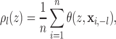
Partial dependence plots are a useful tool for visually assessing the dependence of an estimated function on a particular covariate or set of covariates. As described in Friedman (2001), such plots demonstrate the way an estimated function changes as a particular covariate varies while averaging over the remaining covariates. For the purposes of examining the impact of a covariate on the treatment effects, we define the partial dependence function for the covariate as

where denotes a vector where the component of has been removed and replaced with the value . Estimated partial dependence functions with associated credible bands may be obtained directly from MCMC output. The supplementary material available at Biostatistics online contains a figure showing partial dependence plots for ejection fraction and creatinine, and this figure also displays the posterior distribution of the overall treatment effect in both the male/female subgroups and the subgroups defined by history of myocardial infarction.

4. Simulations studies

To evaluate the performance of the nonparametric, tree-based AFT method, we performed two main simulation studies. An additional simulation study involving randomly generated nonlinear regression functions is described in part C of the supplementary material available at Biostatistics online. For performance related to quantifying HTE, we recorded the following measures: root mean-squared error (RMSE) of the estimated individualized treatment effects, the misclassification proportion (MCprop), i.e. the proportion of patients allocated to the wrong treatment, and the average coverage of the credible intervals. Average coverage proportions are measured as the average coverage over individuals, namely, , for interval estimates .

For the performance measures of RMSE and coverage proportions, we compared our tree-based nonparametric AFT model (NP-AFTree) with the semi-parametric AFT model (SP-AFTree) where the BART model is used for the regression function and the residual distribution is assumed to be Gaussian. In addition, we compared the NP-AFTree procedure with a parametric AFT model (Param-AFT) which assumes a linear regression with treatment-covariate interactions and log-normal residuals. For both the NP-AFTree and SP-AFTree methods, MCMC iterations were used with the first treated as burn-in steps. For both of these, the default parameters (i.e. , , ) were used for each simulation scenario.

4.1. AFT simulations based on the SOLVD trials

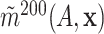In our first set of simulations, we use data from the SOLVD trials (The SOLVD Investigators, 1991) as a guide. To generate our simulated data, we first took two random subsets of sizes and from the SOLVD data. For each subset, we computed estimates and 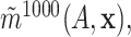respectively of the regression function for using the nonparametric AFT Tree model. Simulated responses were then generated as

(4.1)

where the regression function was fixed across simulation replications and 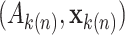corresponds to the patient’s treatment assignment and covariate vector in the random subset with patients. The constant in (4.1) was added so that there was a substantial fraction of simulated patients that would have an underlying ITE less than zero. For the distribution of , we considered four different choices: a Gaussian distribution, a Gumbel distribution with mean zero, a “standardized” Gamma distribution with mean zero, and a mixture of three t-distributions with degrees of freedom for each mixture component. The parameters of these four distributions were chosen so that the variances were approximately equal, and the levels of censoring was varied across three levels: none, light censoring ( of cases censored), and heavy censoring ( of cases censored).

Root mean-squared error, misclassificiation, and coverage results are shown in Figure 3. More detailed results from this simulation study are detailed in part G of the supplementary material available at Biostatistics online. As may be inferred from Figure 3, the NP-AFTree method consistently performs better in terms of RMSE and MCprop than the SP-AFTree procedure. Moreover, while not apparent from the figure, the NP-AFTree approach performs just as well as SP-AFTree, even when the true residual distribution is Gaussian (see the supplementary material available at Biostatistics online). For each residual distribution, the advantage of NP-AFTree over SP-AFTree is more pronounced for the smaller sample sizes settings , with closer performance for the cases. While RMSE and MCprop seem to be comparable between NP-AFTree and SP-AFTree for the settings, the coverage for NP-AFTree is consistently closer to the desired level and is greater than for nearly all settings. When , average coverage often differs substantially from , but in these cases, BART is quite conservative in the sense that coverage is typically much greater than . It is worth mentioning that while we have observed good frequentist coverage in many settings, BART does not come with strong frequentist coverage guarantees as the reported uncertainty measures are based on Bayesian credible intervals. The supplementary material available at Biostatistics online shows an example where modest under coverage has been observed. In our experience, such cases of under coverage can occur when there is both low treatment balance in certain regions of the covariate space and considerable variation in the ITE function . In these cases, the regularization prior used by BART imposes a kind of skepticism on very large ITEs meaning that ITE estimates and credible intervals are shrunken considerably whenever there is not strong evidence supporting ITEs that differ strongly from the overall treatment effect. In other words, under coverage is often due to shrinkage towards the overall treatment effect rather than estimates which overstate the amount of HTE.

Fig. 3.

Simulations based on the SOLVD trial data. Results are based on simulation replications. Root mean-squared error, misclassification proportion, and empirical coverage are shown for each method. Performance measures are shown for the NP-AFTree method, the SP-AFTree, and the parametric, linear regression-based AFT (Param-AFT) approach. Four different choices of the residual distribution were chosen: a Gaussian distribution, a Gumbel distribution with mean zero, a “standardized” Gamma distribution with mean zero, and a mixture of three t-distributions with degrees of freedom for each mixture component.

4.2. Several “null” simulations

We considered data generated from several “null” cases where the simulation scenarios were designed to have no HTE. For these simulations, we consider four AFT models and one Cox proportional-hazards model. In these “null” simulations, we are primarily interested in the degree to which the NP-AFTree procedure “detects” spurious HTE in settings where no HTE is present in the underlying data generating model. The AFT models used for the simulations assumed a linear regression function with no treatment-covariate interactions

(4.2)

and the hazard functions for the Cox model simulations similarly took the form

(4.3)

Although there may be a degree of heterogeneity in for the Cox proportional hazards model (4.3), it is still worthwhile to investigate the behavior of when there is no HTE when treatment effects are defined in terms of hazard ratios.

The parameters in (4.2) were first estimated from the SOLVD data using a parametric AFT model with log-normal residuals. Herein, we estimated the parameters in (4.2) separately using the same fixed subsets of size and used in Section 4.1. The parameters were fixed across simulation replications. For the AFT models, we considered the same four choices of the residual term distribution as in Section 4.1. The parameters for the hazard functions in (4.3) were found by fitting a Cox proportional hazards model to the same two subsets of size and from the SOVLD trials data, and these parameters were fixed across simulation replications. The cumulative baseline hazard function used for generating the Cox proportional hazards simulations was found using Breslow’s estimator.

For each null simulation scenario, we computed the posterior probabilities of differential treatment effect (see equations (3.2) and 3.3)) and tabulated the percentage of patients with either strong evidence of differential treatment effect (i.e. ) or mild evidence (i.e. ). Table 2 shows, for each null simulation scenario, the average proportion of individuals exhibiting strong evidence of a differential treatment effect and the average proportion of individuals exhibiting mild evidence. As displayed in Table 2, the average percentage of individuals showing strong evidence of differential treatment effect is less than for all simulation settings. Moreover, the percentages of cases with mild evidence of differential treatment effect was fairly modest. The average percentage of patients with mild evidence was less than for all except one simulation scenario, and most of the simulation scenarios had, on average, less than of patients exhibiting mild evidence of differential treatment effect. Null simulations with tended to have much fewer cases of strong or mild evidence than those simulations with . The results presented in Table 2 suggest that the NP-AFTree procedure rarely reports any patients as having strong evidence of differential treatment effects in situations where HTE is absent.

Table 2.

Simulation for settings without any HTE present

		Normal		Gumbel		Std-Gamma		T-mixture		Cox-PH
n	Censoring	SE	ME	SE	ME	SE	ME	SE	ME	SE	ME
200	none	0.000	0.095	0.000	0.040	0.000	0.070	0.000	0.060	0.000	0.140
200	light	0.000	0.095	0.000	0.000	0.075	0.350	0.000	0.380	0.000	0.015
200	heavy	0.000	0.020	0.000	0.000	0.000	0.000	0.000	0.055	0.000	0.290
1000	none	0.000	0.803	0.073	2.066	0.092	1.483	0.161	3.087	0.176	3.824
1000	light	0.061	1.989	0.015	0.967	0.213	2.674	0.066	3.176	0.111	3.405
1000	heavy	0.002	1.253	0.000	0.484	0.030	1.176	0.123	2.953	0.135	2.688

Results are based on simulation replications. Average percentage of patients exhibiting strong evidence (SE) of differential treatment effect (i.e. ) and average percentage of patients exhibiting mild evidence (ME) of differential treatment effect (i.e. ). Results are shown for AFT models with the same four residual distributions used in the simulations from Section 4.1 and for a Cox-proportional hazards model with no treatment-covariate interactions. Censoring levels were varied according to: none, light censoring ( of cases censored), and heavy censoring ( of cases censored).

5. Discussion

In this article, we have described a flexible, tree-based approach to examining heterogeneity of treatment effect with survival endpoints. This method produces estimates of individualized treatment effects and corresponding credible intervals for AFT models with an arbitrary regression function and residual distribution. Moreover, we have demonstrated how this approach provides a useful framework for addressing a variety of other HTE-related questions. When using the default hyperparameter settings, the method only requires the user to input the survival outcomes, treatment assignments, and patient covariates. Due to the tree-based formulation of the regression function, the user does not need to pre-specify any treatment covariate interaction terms or patient subgroups in order to obtain informative characterizations of HTE. As shown in several simulation studies, the default settings exhibit strong predictive performance and good coverage properties. Though quite flexible, our nonparametric AFT model does entail some assumptions regarding the manner in which the patient covariates modify the baseline hazard. Hence, it would be worth further investigating the robustness of the nonparametric AFT method to other forms of model misspecification such as cases where neither an AFT or a Cox proportional hazards assumption holds or cases where the residual distribution depends on the patient covariates.

In addition to describing a novel nonparametric AFT model, we examined a number of measures for reporting HTE including the distribution of individualized treatment effects, the proportion of patients benefiting from treatment, and posterior probabilities of differential treatment effect. Each have potential uses in allowing for more refined interpretations of clinical trial results. The argument has been made by some (e.g. Kent and Hayward, 2007) that the positive results of some clinical trials are driven substantially by the outcomes of high-risk patients. In such cases, the posterior distribution of the ITEs along with the estimated proportion benefiting may help in clarifying the degree to which lower risk patients are expected to benefit from the proposed treatment. In Section 4.2, we explored the use of posterior probabilities of differential treatment effect as a means of detecting the presence of HTE. Such measures show potential for evaluating the consistency of treatment and for assessing whether or not further investigations into HTE are warranted.

6. Software

The methods described in this paper are implemented in the R package AFTrees, which is available for download at https://github.com/nchenderson/AFTrees (accessed July 4, 2018). The AFTrees package and additional supplementary code is also available for download at http://hteguru.com/index.php/software/ (accessed July 4, 2018).

Funding

The authors were supported by the National Institute of Health’s (NIH) National Center for the Advancement of Translational Sciences (NCATS) through the grant number UL1TR001079-04S1, and by the NIH grant number P30CA006973. This work was also supported through a Patient-Centered Outcomes Research Institute (PCORI) Award (ME-1303-5896).

References

- Bonato, V., Baladandayuthapani, V., Broom, B. M., Sulman, E. P., Aldape, K. D. and Do, K.-A. (2011). Bayesian ensemble methods for survival prediction in gene expression data. Bioinformatics 27, 359–367. [DOI] [PMC free article] [PubMed] [Google Scholar]
- Chipman, H. A., George, E. I. and McCulloch, R. E. (1998). Bayesian CART model search (with discussion and a rejoinder by the authors). Journal of the American Statistical Association 93, 935–960. [Google Scholar]
- Chipman, H. A., George, E. I. and McCulloch, R. E. (2010). BART: Bayesian additive regression trees. The Annals of Applied Statistics 4, 266–298. [Google Scholar]
- Chipman, H. and McCulloch, R. (2016). BayesTree: Bayesian Additive Regression Trees. R package version 0.3-1.4. [Google Scholar]
- Foster, J. C., Taylor, J. M. G. and Ruberg, S. J. (2011). Subgroup identification from randomized clinical trial data. Statistics in Medicine 30, 2867–2880. [DOI] [PMC free article] [PubMed] [Google Scholar]
- Friedman, J. (2001). Greedy function approximation: a gradient boosting machine. The Annals of Statistics 29, 1189–1232. [Google Scholar]
- Hanson, T. and Johnson, W. O. (2002). Modeling regression error with a mixture of Polya trees. Journal of the American Statistical Association 97, 1020–1033. [Google Scholar]
- Hanson, T. E. (2006). Modeling censored lifetime data using a mixture of gammas baseline. Bayesian Analysis 1, 575–594. [Google Scholar]
- Hill, J. L. (2011). Bayesian nonparametric modeling for causal inference. Journal of Computational and Graphical Statistics 20, 217–240. [Google Scholar]
- Ishwaran, H. and James, L. F. (2001). Gibbs sampling methods for stick-breaking priors. Journal of the American Statistical Association 96, 161–173. [Google Scholar]
- Johnson, W. and Christensen, R. (1988). Modeling accelerated failure time with a Dirichlet process. Biometrika 75, 693–704. [Google Scholar]
- Jones, H. E., Ohlssen, D. I., Neuenschwander, B., Racine, A. and Branson, M. (2011). Bayesian models for subgroup analysis in clinical trials. Clinical Trials 8, 129–143. [DOI] [PubMed] [Google Scholar]
- Kent, D. M. and Hayward, R. A. (2007). Limitations of applying summary results of clinical trials to individual patients - The need for risk stratification. Journal of the American Medical Association 298, 1209–1212. [DOI] [PubMed] [Google Scholar]
- Komárek, A. and Lesaffre, E. (2007). Bayesian accelerated failure time model for correlated interval-censored data with a normal mixture as error distribution. Statistica Sinica 17, 549–569. [Google Scholar]
- Komárek, A., Lesaffre, E. and Hilton, J. F. (2005). Accelerated failure time model for arbitrarily censored data with smoothed error distribution. Journal of Computational and Graphical Statistics 14, 726–745. [Google Scholar]
- Kuo, L. and Mallick, B. (1997). Bayesian semiparametric inference for the accelerated failure-time model. The Canadian Journal of Statistics 25, 457–472. [Google Scholar]
- Lamont, A., Lyons, M. D., Jaki, T., Stuart, E., Feaster, D. J., Tharmaratnam, K., Oberski, D., Ishwaran, H., Wilson, D. K. and Horn, M. L. V. (2018). Identification of predicted individual treatment effects in randomized clinical trials. Statistical Methods in Medical Research 27, 142–157. [DOI] [PubMed] [Google Scholar]
- Loh, W.-Y., He, X. and Man, M. (2015). A regression tree approach to identifying subgroups with differential treatment effects. Statistics in Medicine 34, 1818–1833. [DOI] [PMC free article] [PubMed] [Google Scholar]
- Louis, T. A. and Shen, W. (1999). Innovations in Bayes and empirical Bayes methods: estimating parameters, populations, and ranks. Statistics in Medicine 18, 2493–2505. [DOI] [PubMed] [Google Scholar]
- Shen, Y. and Cai, T. (2016). Identifying predictive markers for personalized treatment selection. Biometrics 72, 1017–1025. [DOI] [PMC free article] [PubMed] [Google Scholar]
- Sparapani, R. A., Logan, B. R., McCulloch, R. E. and Laud, P. W. (2016). Nonparametric survival analysis using Bayesian additive regression trees (BART). Statistics in Medicine 35, 2741–2753. [DOI] [PMC free article] [PubMed] [Google Scholar]
- Su, X., Tsai, C.-L., Wang, H., Nickerson, D. M. and Li, B. (2009). Subgroup analysis via recursive partitioning. Journal of Machine Learning Research 10, 141–158. [Google Scholar]
- The SOLVD Investigators. (1991). Effect of enalapril on survival in patients with reduced left ventricular ejection fraction and congestive heart failure. The New England Journal of Medicine 325(5), 293–302. [DOI] [PubMed] [Google Scholar]
- Wager, S. and Athey, S. (2015). Estimation and inference of heterogeneous treatment effects using random forests. ArXiv 1510.04342. [Google Scholar]
- Wager, S., Hastie, T. and Efron, B. (2014). Confidence intervals for random forests: the jackknife and the infinitesimal jackknife. Journal of Machine Learning Research 15, 1625–1651. [PMC free article] [PubMed] [Google Scholar]
- Wei, L. J. (1992). The accelerated failure time model: a useful alternative to the Cox regression model in survival analysis. Statistics in Medicine 11, 1871–1879. [DOI] [PubMed] [Google Scholar]
- Weisberg, H. I. and Pontes, V. P. (2015). Post hoc subgroups in clinical trials: anathema or analytics? Clinical Trials 12, 357–364. [DOI] [PubMed] [Google Scholar]
- Xu, Y., Yu, M., Zhao, Y.-Q., Li, Q., Wang, S. and Shao, J. (2015). Regularized outcome weighted subgroup identification for differential treatment effects. Biometrics 71, 645–653. [DOI] [PMC free article] [PubMed] [Google Scholar]
- Yang, M., Dunson, D. B. and Baird, D. (2010). Semiparametric Bayes hierarchical models with mean and variance constraints. Computational Statistics & Data Analysis 54, 2172–2186. [DOI] [PMC free article] [PubMed] [Google Scholar]
- Zhao, Y.-Q., Zheng, D., Rush, A. J. and Kosorok, M. R. (2012). Estimating individualized treatment rules using outcome weighted learning. Journal of the American Statistical Association 107, 1106–1118. [DOI] [PMC free article] [PubMed] [Google Scholar]
Associated Data
This section collects any data citations, data availability statements, or supplementary materials included in this article.