

Abstract
Hot and humid heat exposures challenge the health of outdoor workers engaged in occupations such as construction, agriculture, first response, manufacturing, military, or resource extraction. Therefore, government institutes developed guidelines to prevent heat‐related illnesses and death during high heat exposures. The guidelines use Wet Bulb Globe Temperature (WBGT), which integrates temperature, humidity, solar radiation, and wind speed. However, occupational heat exposure guidelines cannot be readily applied to outdoor work places due to limited WBGT validation studies. In recent years, institutions have started providing experimental WBGT forecasts. These experimental products are continually being refined and have been minimally validated with ground‐based observations. This study evaluated a modified WBGT hindcast using the historical National Digital Forecast Database and the European Centre for Medium‐Range Weather Forecasts Reanalysis v5. We verified the hindcasts with hourly WBGT estimated from ground‐based weather observations. After controlling for geographic attributes and temporal trends, the average difference between the hindcast and in situ data varied from −0.64°C to 1.46°C for different Köppen‐Geiger climate regions, and the average differences are reliable for decision making. However, the results showed statistically significant variances according to geographical features such as aspect, coastal proximity, land use, topographic position index, and Köppen‐Geiger climate categories. The largest absolute difference was observed in the arid desert climates (1.46: 95% CI: 1.45, 1.47), including some parts of Nevada, Arizona, Colorado, and New Mexico. This research investigates geographic factors associated with systematic WBGT differences and points toward ways future forecasts may be statistically adjusted to improve accuracy.
Keywords: climate change adaptation, heat exposure, weather forecast, occupational exposure
Key Points
The estimated Wet Bulb Globe Temperature seems to be reliable for most parts of the U.S.
The differences varied according to geographical features, temporal variables, and the Köppen‐Geiger climatic zones
The estimated average differences varied from −0.64°C to 1.46°C according to the Köppen‐Geiger climate categories
1. Introduction
Hot and humid heat exposures challenge the health of outdoor workers engaged in such as construction, agriculture, first response, manufacturing, military, or resource extraction. Furthermore, workers produce additional metabolic heat through exertional activity, coping with radiant heat from machines, and may wear heat‐insulating protective equipment (Cai et al., 2019; Vega‐Arroyo et al., 2019). Elevated heat exposure increases the risk of deaths, illnesses, and injuries among outdoor workers and reduces workers' productivity and cognitive functioning (Garzon‐Villalba et al., 2016; Riley et al., 2012, 2018; Spector & Sheffield, 2014; Varghese et al., 2019; Venugopal et al., 2019).
Most outdoor heat‐related deaths can be prevented with occupational and exertional heat management practices (Arbury et al., 2016; Hosokawa et al., 2019; Lemke et al., 2019). For example, the State of California Department of Industrial Regulation (2018) requires outdoor workers to take breaks in the shade and rehydrate when air temperatures exceed 80 degrees Fahrenheit (26.6°C). In addition to air temperature, previous studies have found that wind speed, solar radiation, and humidity influence heat exposure and the human body's ability to thermoregulate. Therefore, many guidelines are based on Wet Bulb Globe Temperature (WBGT), which integrates a broader suite of physical characteristics and is more applicable to outdoor workers than heat index, which is calculated with relative humidity and air temperature. Multiple occupational heat exposure and safety guidelines use WBGT to determine the intensity of work and duration of rest that can be safely completed (American College of Sports Medicine, 2012; Occupational Safety and Health, 2016; Occupational Safety and Health Administration, 2014; U.S. Department of Defense, 2003). The U.S. National Oceanic and Atmospheric Administration National Weather Service (NOAA NWS) started to issue experimental WBGT forecasts using the National Digital Forecast Database (NDFD), which is generated by regional Weather Forecast Offices (WFOs). This NOAA NWS WBGT forecast is experimental and is continually refined by feedback from NWS teams. However, few studies have investigated the difference between simulated WBGT and observed WBGT. Thus, this study's overarching purpose was to validate a modified hindcasted WBGT calculated from historical NDFD with WBGT estimated from ground‐based weather stations across the continental U.S. from 2018 to 2019.
Much of the research suggested an association between weather conditions and geographical variables (Behnke et al., 2016; Daly et al., 2008; Rubel et al., 2017). For example, many studies have found the local climate is altered by coastal effects (Daly et al., 2008; Fleuret & Atkinson, 2007), local land use and land cover (Davey & Pielke, 2005) and topographical features (Behnke et al., 2016; Daly et al., 2008; Myrick & Horel, 2006; Zardi & Whiteman, 2013). Therefore, we considered the following geographical features that should theoretically influence WBGT statistical biases: elevation, slope, aspect, land cover, local topographic features, distance from the coastline, and climate division information. On the windward side of a mountain, moisture saturation and precipitation increase, and air temperature decrease as the elevation increases (Behnke et al., 2016; Daly et al., 2008). A large number of studies found that wind direction and air flows vary in accordance with features of terrain such as valley bottom, mid‐slope, or ridge top (Albergel et al., 2018; Daly et al., 2008; Myrick & Horel, 2006; Page et al., 2018; Zardi & Whiteman, 2013). Therefore, we will consider geographical features and climate zones to answer the following questions: (a) To what extent can systematic WBGT errors be explained by local geographic patterns and temporal cycles; and (b) Which climatic zones have the strongest/weakest association with the difference between estimated and in situ WBGT?
2. Method
2.1. Scope of Study
This study focuses on the “warm” seasons (from April to October) of 2018–2019 during the “daylight” hours (05–21) in the 48 continental states in the United States.
2.2. Gridded Weather Data for Estimated WBGT
2.2.1. National Digital Forecast Database
The NDFD was developed to efficiently provide weather information to the Weather Enterprise (e.g., academia, government, and private industry). The NDFD currently has a gridded horizontal resolution of 2.5 km and data from NDFD are available at the National Centers for Environmental Information (NCEI) website (National Centers for Environmental Information (NCEI), 2021). Expert forecasters can consider local and regional terrain to predict the NDFD at local WFOs (Page et al., 2018). NDFD is updated every 30 min when new, and revised digital data from the WFO or NOAA National Centers for Environmental Prediction becomes available. This study used the NDFD model's historical temperature, dew point temperature, wind speed (10 m above ground), and relative humidity variables. However, the NDFD provides cloud cover but not solar radiation values, which is a crucial variable for estimating WBGT. The NOAA NWS process of estimating solar radiation evolved over the course of this project. While the experimental forecasts using Dimiceli et al.'s (2013) algorithm were not available until 2019, the historical NDFD forecasts (which do not include solar radiation) were systematically archived. To complement the NDFD, we gathered solar radiation data from the European Centre for Medium‐Range Weather Forecasts Reanalysis v5 (ERA5) which provided relatively accurate and accessible and comprehensive weather information (Tang et al., 2019).
2.2.2. ERA5
ERA5 provides an hourly forecast of approximately 300 atmospheric, land, and oceanic weather variables. The data is continuously updated within 5 days of real‐time, and the data has a horizontal spatial resolution of 30 km. For this study, the model provided hourly surface solar radiation (Tang et al., 2019). The data is available at the European Centre for Medium‐Range Weather Forecasts website (European Centre for Medium‐Range Weather Forecasts, 2021).
2.3. In Situ Weather Data for Observed WBGT
2.3.1. Data Collection
We collected historical in situ weather information from a patchwork of institutions due to the limited number of NOAA NCEI stations that recorded downward hourly solar radiation. Figure 1 provides the names of organizations that shared observational weather data free of charge for research purposes from 1,152 nationwide stations across 40 states (Table A1) (Colorado State University, 2020; Cooperative Agriculture Weather Network, 2020; Illinois State, 2019; Kansas Mesonet, 2017; Michigan State University, 2020; Missouri Mesonet, 2020; North Carolina State University, 2020; North Dakota Agriculture Weather Network Center, 2020; South Alabama, 2020; STEM, 2020; University of Arizona, 2020; University of Florida, 2020).
Figure 1.
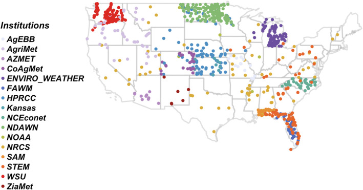
Location of stations. Note. Following information indicates abbreviation of the institutes and number of stations in the parentheses. AgEBB, Commercial Agriculture Program, Missouri University (29); AgriMet, Cooperative Agriculture Weather Network (28); AZMET, The Arizona Meteorological Network (83); CoAgMet, Colorado Agricultural Meteorological Network (77); ENVIRO_WEATHER, Michigan State University (95); FAWM, Florida Automated Weather Network (42); HPRCC, High Plains Regional Climate Center (113); Kansas, Kansas Mesonet (17); NCE CoNet:North Carolina Climate Office (39); NDAWN, North Dakota Agricultural Weather Network (152); NOAA:National Oceanic and Atmospheric Administration (6); NRCS, Natural Resources Conservation Service (138); SAM, South Alabama Mesonet (23); STEM:Weather STEM (141); WARM, Illinois Water and Atmospheric Resources (6); WSU, Washington State University (160); ZiaMet, New Mexico State University (10).
2.3.2. Quality Control for In Situ Data
We applied a statistically based quality control (QC) method to filter out suspicious observations (Napoly et al., 2018). We first flagged hourly WBGT outliers by identifying observations with z‐scores within the upper or lower 0.5% of all hourly WBGT data across the study period (Grassmann et al., 2018). If more than 20% of a station's observations in a month were flagged, QC removed the entire month's data. Furthermore, if a station was missing more than 20% of its study months, it was considered potentially erroneous, and the station was dropped from the study (Napoly et al., 2018). Through this process, 41% of the total station months were removed. Of the 1,152 candidate stations, 622 (53.9%) were used for the analysis. The number of stations that were included by year and month is indicated in Table A2. The stations were geographically distributed throughout the nation as follows; the Midwest and Great Plains had 270, the Northeast had 4, the South had 118, and the West had 230. The stations provided hourly solar radiation, air temperature, wind speed, and dew point temperature or relative humidity (Figure 1).
2.4. Geographical Data Collection
Many studies suggest that regions' topography such as large water bodies, the proximity to the ocean, land use, and influences local climatic conditions (Albergel et al., 2018; Daly et al., 2008; I. Gultepe et al., 2014; Oke, 1982). In addition, companion studies suggest gridded historical weather data's accuracy varies based on each regional climate zone (Behnke et al., 2016). Therefore, the analysis included elevation and terrain information from a 30 m resolution digital elevation model (NASA, 2007). Validation studies found the vertical height error was less than 16 m (Cooper et al., 2006). The US NED Multi‐Scale Topographic Position Index (mTPI) from Conservation Science Partners (Conservation Science Partners (CSP), 2020; Theobald et al., 2015) and accessed via Google Earth Engine inferred whether in situ stations were located in a ridge or a valley. Validation studies suggest the mTPI (m/km) is highly correlated with the spatial rate of temperature changes (°C/km) which showed Pearson's correlation 0.792 (Theobald et al., 2015). Positive values correspond to ridges and negative values to valleys. Moreover, Daly et al. (2008) suggest land use and land cover influence the local climate of gridded weather products. Intuitively, land use and land cover alter heat, moisture, and momentum fluxes (Behnke et al., 2016; Daly et al., 2008; Eliasson & Svensson, 2003; Geiger, Aron, and Todhunter, 2009; Myrick & Horel, 2006). This study used the United States Geological Survey (USGS) National Land Cover Database (NLCD) CONUS 2016 (United States Geological Survey (USGS), 2016). NLCD data was derived from an unsupervised classification of 30‐m Landsat data that has an overall classification accuracy of 88% (L. Yang et al., 2018).
We included coastal proximity information based on previous studies' findings of the influence of large water bodies and local sea breeze dynamics (Daly et al., 2008). The coastal proximity was collected from a 1:1,000,000‐map Scale Coastline of the United States (United States Geological Survey (USGS), 2014) by calculating the minimum distance from each individual in situ station's location with the “geopandas” package in Python 3.7 (Jordahl et al., 2021). Coastal influences diminish over distances from 1 to 50 km. In the summertime, the temperature differences between inland and coast can exceed 20 degrees Celsius within 5–20 km from the coastline (Daly et al., 2002; Perry & Hollis, 2005). Therefore, we indicated the stations that are located within 5 km as a compromise between local coastal and sea breeze effects.
We included the Köppen‐Geiger climate classification to consider the variations of the WBGT among different climate zones. Beck et al. (2018) updated global maps of the Köppen‐Geiger climate classification at a 1‐km resolution for a contemporary climatology period (1980–2016) (Table 1). The Köppen‐Geiger climate classification is based on mean temperature and precipitation. The continental US has 19 different climate zones.
Table 1.
Geographical Variables and Data Sources
| Data name | Variables | Data type | Categories | Data source |
|---|---|---|---|---|
| 30 M Digital Elevation Map | Elevation | Continuous | N/A | NASA (2007); Farr et al. (2007) |
| 30 M DEM | Aspect | Categorical | East, flat, north, northeast, southwest, south, southwest, west, northwest, and north | NASA (2007); Farr et al. (2007) |
| National Land Cover Database (NLCD) | Land use | Categorical | Open water developed open space, developed low intensity, developed medium intensity, developed high intensity, barren land (rock/sand/clay), deciduous forest, evergreen forest, mixed forest, shrub/scrub, grassland/herbaceous, pasture/hay, cultivated crops, woody wetlands, emergent herbaceous wetlands | United States Geological Survey (USGS) (2016) and Yang et al. (2018) |
| US NED mTPI (Multi‐Scale Topographic Position Index) | Topographic Position Index | Categorical | Ridge and valley index (1: ridge, 0: valley) | Conservation Science Partners (CSP) (2020) and Theobal et al. (2015) |
| 1:1,000,000‐Scale Coastline of the United States | Coastal proximity | Categorical | Distance from the coastline (1: within 5 km, 0: outside 5 km) | United States Geological Survey (USGS) (2014) |
| Köppen‐Geiger climate classification | Köppen‐Geiger climate classification | Tropical (Af, Am, Aw), arid steppe (BSh, BSk), arid desert (BWh, BWk), temperate (Cfa, Csb, Csa, Cfb), cold and no dry season (Dfa, Dfb), and cold and dry (Dsa, Dsb, Dwa, Dwb) | Beck et al. (2018) |
2.5. Data Processing
2.5.1. Wet Bulb Globe Temperature Estimation
WBGT is a relatively conservative measure of heat exposure that increases the risk of occupational injury or heat‐related illness (Yaglou & Minaed, 1957).
| (1) |
In Equation 1, WBGT is the weighted sum of natural wet bulb temperature (T nw), black globe temperature (T g), and ambient air temperature (T a ). Natural wet bulb temperature is directly related to air temperature and humidity and indirectly to wind speed and radiation. Black globe temperature is influenced by solar and thermal radiation and wind speed via convective cooling. Thus, WBGT captures physical processes (conduction, convection, radiation, and evaporation) that influence the human body's thermoregulation.
This study analyzed WBGT estimated from NOAA NWS's NDFD (hourly air temperature, dew point temperature, wind speed at 10m) and hourly solar radiation from ERA reanalysis (est_WBGT). We estimated 2 m from 10m wind speeds using a vertical wind profile power law for a radiatively cooled rural area (stability class C) (Liljegren et al., 2008). We compared hourly est_WBGT with in situ_WBGT from the observation weather information. There are multiple thermodynamic and/or derived empirical methods to approximate WBGT based on weather observations (Gaspar & Quintela, 2009; Hunter & Minyard, 1999). We choose Liljegren et al.'s (2008) approach since inter‐comparison studies suggest the two most common algorithms (Dimiceli et al., 2013; Liljegren et al., 2008) perform well across different climatic zones (Lemke & Kjellstrom, 2012; Patel et al., 2013; Rennie et al., 2021).
The “HeatStress” package in R implements Liljegren et al.'s (2008) algorithm to convert weather information to WBGT for both est_WBGT and in situ_WBGT. The function requires air temperature, relative humidity, solar radiation, and dewpoint temperature. Some weather stations from SAM, FAWM, ENVIRO, Kansas, AgEBB, and CoAgMet provided relative humidity, which was subsequently converted to dew point temperature using the “meteocalc” package in Python 3.7.
2.6. Analysis
The aim of the analysis was to examine which geographic variables were associated with the difference between est_WBGT and in situ_WBGT (dependent variable). We constructed a Gaussian distribution mixed‐effects model with a random effect to control for stations nested within climate regions using the “lme4” R statistical computing package (Casa et al., 2015). The hourly difference was calculated during the warm season (April to October) and potential daylight hours (5 a.m. to 9 p.m.). The study focused on the WBGT difference to illustrate how the statistical corrections could improve accuracy. The independent variables were elevation, aspect, topographic position index, land use, location within 5 km from coastline, month, and beta spline of the hour of the day and month of the year. WBGT, elevation, and hour of the day were modeled as continuous variables, while the remaining independent variables were categorical (Table 1).
To consider the diurnal and annual WBGT cycle, we created a beta‐spline basis with 3‐degrees of freedom for the hour of the day and month of the year with the “splines” package (version 4.0.2) in R (R Development Core Team, 2010). Splines use piecewise polynomial functions to model non‐linear cycles. We modeled stations nested within Köppen‐Geiger climate zones with a random effect to estimate a region‐specific statistical bias. Due to the somewhat small number of stations within some regions and a moderately large number of independent variables, the mixed‐effects models were fit by Restricted Maximum Likelihood (Zuur et al., 2010). We recategorized the land use category as well based on microclimate and similar effects on WBGT statistical biases. We merged “pasture and hay” and “grassland and herbaceous” to “Herbaceous” and “Wood wetlands” and “Emergent herbaceous wetlands” to “Wetlands”. We also applied interaction terms between the month of the year and each land category to consider seasonally varying land use effects. We conducted the ANOVA test to compare the interaction between land use and month and applied the interaction term. We confirmed the model's normality of residuals and homogeneity of variance and reported the Akaike Information Criterion (AIC).
Additionally, we examined the effect of geographical features by comparing the AIC between a null model and the full model. We created a null model with an intercept and against the difference between est_WBGT and in situ_WBGT (absolute value of est_WBGT minuses in situ_WBGT). Then, we computed the variance of both null and full models with the AIC function (Chambers & Hastie, 1992). We also compared the null and full model's AIC as a metric of the benefits of considering local geographic characteristics for estimating WBGT.
3. Results
3.1. Descriptive Statistics
Florida has the highest average monthly WBGT (26.8°C) among 40 continental states with observational information. Montana has the lowest monthly average WBGT (1.65°C). The most significant monthly difference between est_WBGT and in situ_WBGT was shown in Vermont (7.22°C). Figure 2 displays each individual station's monthly max and the difference value.
Figure 2.
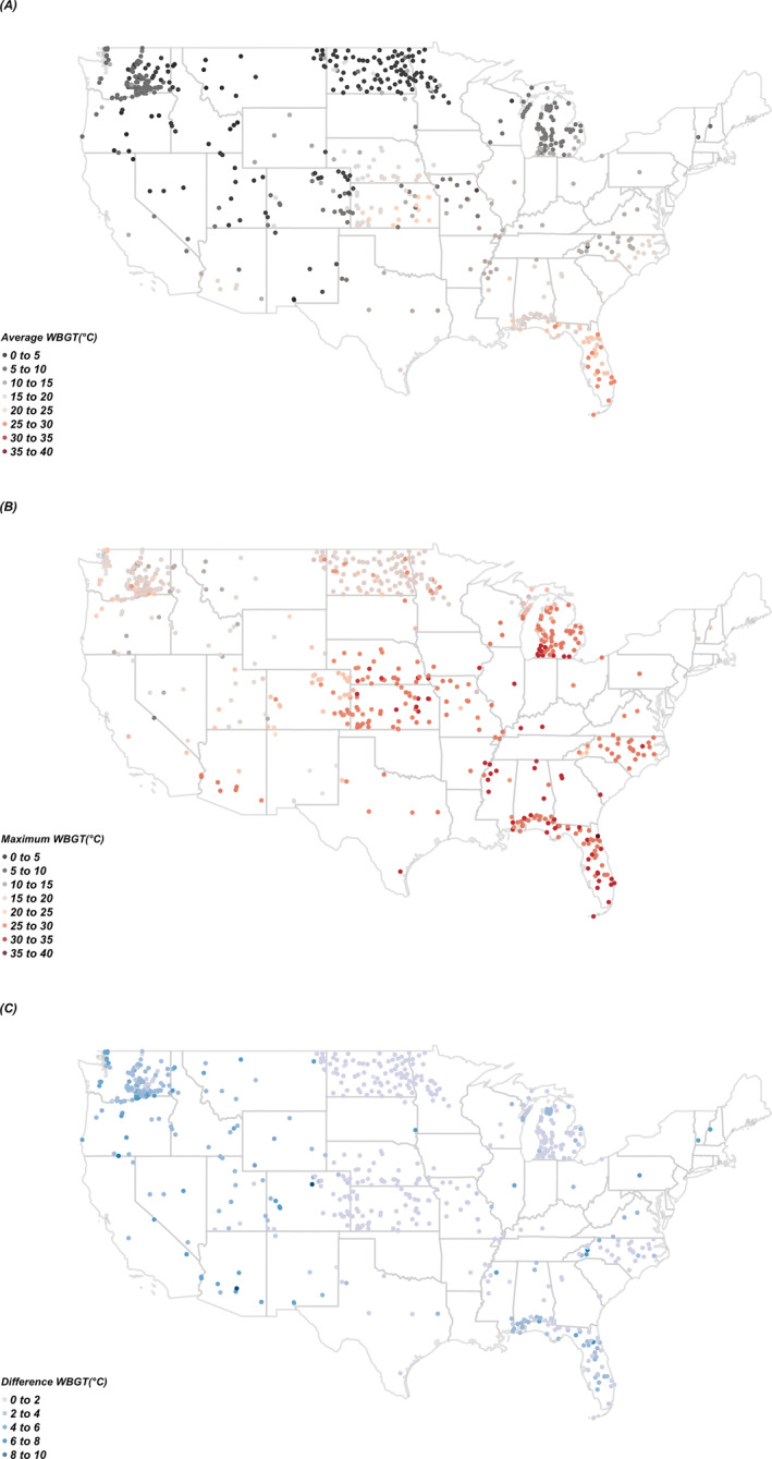
Each individual station's monthly max, and difference value ((a) average Wet Bulb Globe Temperature (WBGT), (b) maximum WBGT, (c) average difference between est_WBGT and obs_WBGT). (Maximum, average difference were calculated from each state's monthly average, maximum and average difference between est_WBGT and in situ_WBGT).
This section summarizes the station locations' local land cover and coastal proximity. The stations were located in 12 out of 20 land use categories. Approximately half of the study stations (54.6%) were in cultivated cropland. More than 10% of stations (26.3%) were located in herbaceous. Other stations were in shrub/scrub (7.6%), developed high intensity (1.9%), evergreen forest (2.3%), deciduous forest (2.3%), wetlands (2.4%), open water (1.6%), barren land (0.6%), and mixed forest (0.5%). Moreover, among the stations we gathered, 3.1% of stations are located within 5 km from the coast.
With the Köppen‐Geiger climate classification, we report how many stations were located in each multi‐class climate zone. The stations were located in 18 out of 19 continental U.S. classifications (Beck et al., 2018). The study subsequently grouped the climate categories into six more general climate regions to increase the number of stations per region (Figure 3). The stations were located in the Cold, no dry season (4.8%), Temperate (21.3%), and Arid steppe (12.6%) climate groups. Reflecting the proportion of the U.S. covered by each climate group, there were a small number of stations in Cold dry (4.8%) and Tropical climates (0.8%) (Table 2).
Figure 3.
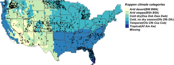
Köppen‐Geiger climate map with station location (Köppen‐Geiger climate map is created based on Beck et al. (2018)).
Table 2.
Number of Stations According to Köppen‐Geiger Climate
| Köppen‐Geiger climate group | Köppen‐Geiger climate categories | Abbreviation | Number of stations (%) | Köppen‐Geiger climate group summary (%) |
|---|---|---|---|---|
| Tropical | Tropical, rainforest | Af | 1 (0.16) | 5 (0.8) |
| Tropical, monsoon | Am | 2 (0.32) | ||
| Tropical, Savannah | Aw | 2 (0.32) | ||
| Arid steppe | Arid, steppe, hot | BSh | 2 (0.32) | 147 (23.7) |
| Arid, steppe, cold | BSk | 145 (23.35) | ||
| Arid desert | Arid, desert, hot | BWh | 6 (0.97) | 78 (12.6) |
| Arid, desert, cold | BWk | 72 (11.59) | ||
| Temperate | Temperate, no dry season, hot summer | Cfa | 110 (17.71) | 132 (21.3%) |
| Temperate, no dry season, warm summer | Cfb | 5 (0.81) | ||
| Temperate, dry summer, hot summer | Csa | 1 (0.16) | ||
| Temperate, dry summer, warm summer | Csb | 16 (2.58) | ||
| Cold, no dry season | Cold, no dry season, hot summer | Dfa | 119 (19.16) | 229 (36.9) |
| Cold, no dry season, warm summer | Dfb | 109 (17.55) | ||
| Cold, no dry season, cold summer | Dfc | 1 (0.16) | ||
| Cold dry | Cold, dry summer, warm summer | Dsb | 14 (2.25) | 30 (4.8) |
| Cold, dry winter, hot summer | Dwa | 3 (0.48) | ||
| Cold, dry winter, warm summer | Dwb | 13 (2.09) |
3.2. In Situ_WBGT and est_WBGT Relationship
We examined how incorporating geographical variables can further adjust for differences by comparing the null model and full model. The null model had a substantially higher AIC than the full model, suggesting that geographical variables could further improve accuracy between in situ_WBGT and est_WBGT (delta AIC: 321,855.2, df = 55). The mean absolute error, which is the absolute difference between observed and fitted values of the null model and full model was 2.97°C WBGT.
We found a statistically significant association between the geographic variables and differences between est_WBGT and in situ_WBGT. Through these results, we found that aspect, coastal proximity, time of the day, land use, the month of the year (May, June, July, August, and September), and the topographic position index showed a statistically significant relationship with the WBGT difference. We also discovered a significant effect of the month on land use (df = 24, deviance 10,282,188, p < 0.05).
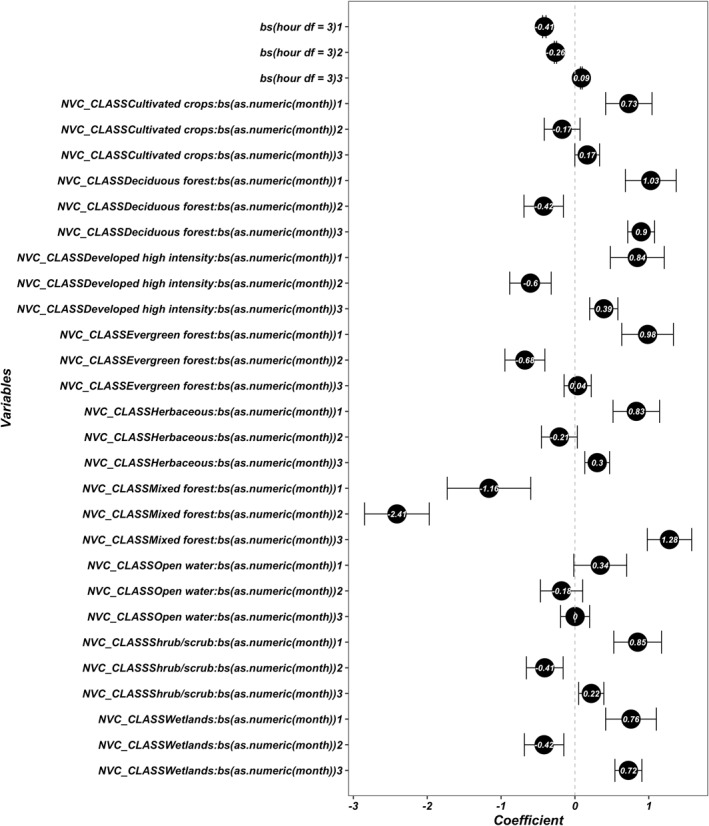
The absolute difference between est_WBGT and in situ_WBGT was bigger at locations within 5 km (0.75, 95% CI: 0.73, 0.75) from the coast. The difference tended to be bigger in valleys than ridges (−0.23, 95% CI: −0.24, −0.23). Except for wetlands, most land use type WBGT difference was bigger compared to barren land. Mixed forest tended to have 1.95 more significant differences than barren land. High intensity tended to have 0.12 bigger difference than barren land (Figure 4). The results showed that the difference between est_WBGT and in situ_WBGT varied throughout the day (Figure 5a). The differences tend to be smaller around noon but larger in the morning (5–10 hr) and afternoon (13–21 hr). The relationship between month of the year and the absolute difference of simulated and in situ WBGT tended to be bigger from April to July and October. Among the land use category, mixed forest showed the biggest difference throughout the year, and other land use showed similar trends (Figure 5b).
Figure 4.
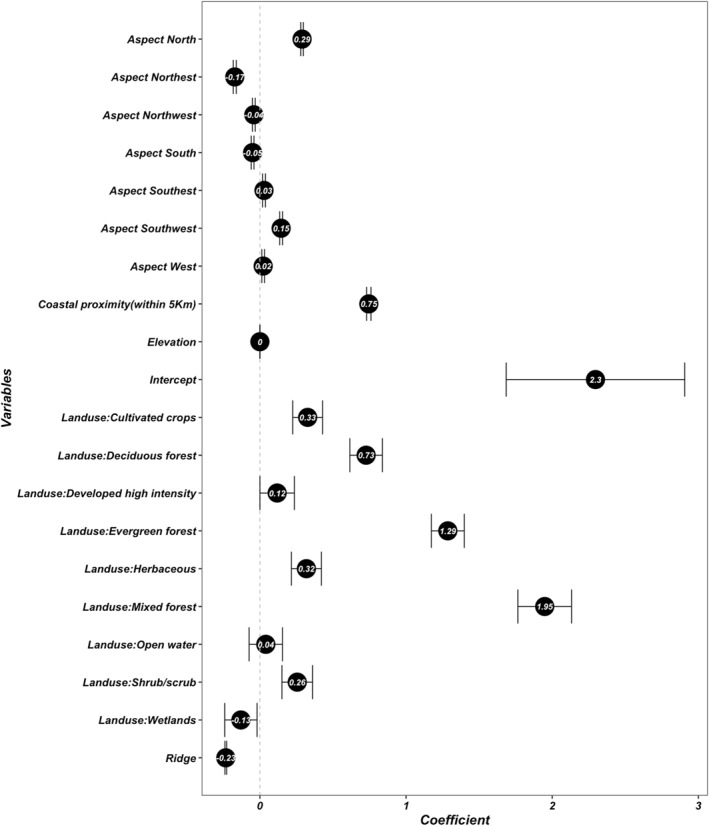
Regression coefficients and the 95% confidence intervals for the difference between estimated and observed Wet Bulb Globe Temperature.
Figure 5.
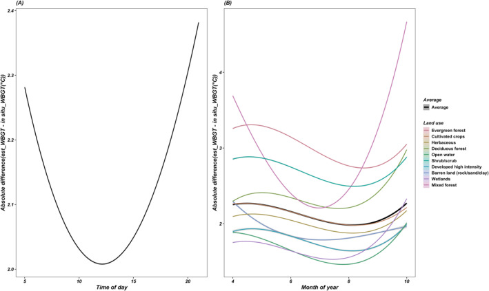
Relationship between the time of day and month of year and absolute difference between simulated and in situ Wet Bulb Globe Temperature (absolute value of est_WBGT—in situ_WBGT) ((a) time of day and (b) month of year according to landsue).
The WBGT difference also varied according to Köppen‐Geiger climate categories (Figure 6). Except for tropical climate, the differences were statistically significant. The biggest differences were shown in the arid desert climates (1.46: 95% CI: 1.45,1 .47). The magnitude of this difference was higher than any other climate zone. The map illustrates that the arid climate areas in Washington, California, Nevada, Utah, Arizona, New Mexico, and Texas states have the biggest differences. The rest of the areas seem to have a 0.1°C–0.6°C difference. The NDFD forecasts overestimated WBGT in Cold and no dry climate (−0.64; 95% CI: −0.65, −0.64), Cold and dry climate −0.46; 95% CI: −0.47, −0.45), and Arid steppe (−0.12; 95% CI: −0.12, −0.11). We also visualized the difference between predicted value from the model and input data (absolute value of simulated WBGT minus in situ WBGT) to illustrate the relative importance of region‐to‐region and within region (Figure 7). The average difference was 0.69°C WBGT across the US. One station showed 7°C difference in Colorado state, 4°C–5°C difference was shown from 6 stations.
Figure 6.
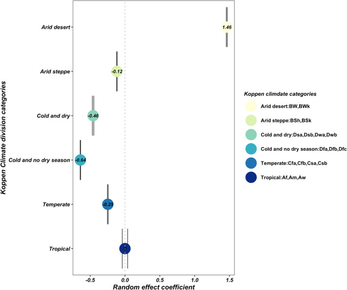
Random effect coefficient.
Figure 7.
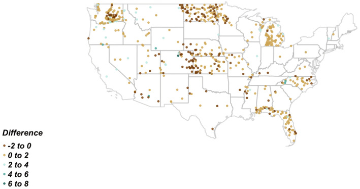
Difference between model predicted value and input data (absolute value of simulated Wet Bulb Globe Temperature (WBGT) minus in situ WBGT.
4. Discussion
The results suggest that the forecasts can be statistically improved by considering geographical features such as land use, topography, and distance from the coasts (Daly et al., 2008). This analysis illustrates the added value of geographical and temporal variables to decrease the discrepancy between in situ_WBGT and est_WBGT. The results showed statistically significant statistical biases according to aspect, coastal proximity, land use, topographic position index, and Köppen‐Geiger climate categories.
This section contextualizes the aspect and topographic position index study results in the broader literature. Mountain climates' dynamics are affected by slope, aspect, radiation, heat, cloudiness, wind, and precipitation (Barry, 2008; Du Vivier & Cassano, 2013; Gultepe, 2015; I. Gultepe et al., 2014; Kilpelainen et al., 2011; Monson & Baldocchi, 2014; Reeve & Kolstad, 2011). Previous studies have shown topography creates local airflows such as cold air drainage, adiabatic cooling, and diurnal mountain wind (Zardi & Whiteman, 2013). These processes can be challenging to model due to the complex terrain, differential solar heating, and wind speeds (Albergel et al., 2018; Page et al., 2018; Zardi & Whiteman, 2013). A previous NDFD validation study found the largest discrepancies between NDFD and observed wind speeds in complex terrain such as Colorado (Myrick & Horel, 2006). Colle et al.'s (2003) study of the dynamically downscaled Eta Model similarly found comparatively large wind speed statistical biases over the Rocky Mountains and western plains. Slater's (2016) research also found accounting for topography improved daily solar radiation predictions.
Moreover, we discovered significant differences in land use and land cover, which aligns with several published studies (Bonan, 1997; Chen et al., 2011; Eliasson & Svensson, 2003; Oke, 1973, 1982). The biosphere and atmosphere interact through heat, water, and energy fluxes that theoretically cause discrepancies between observed and est_WBGT (Monson, 2014; Monson & Baldocchi, 2014; Pielke et al., 1991). In urban areas, air temperature can be 9°C warmer than surrounding areas due to impervious surfaces, air pollution, and tall buildings (Eliasson & Svensson, 2003; Oke, 1973, 1982).
Stations close to the coastline tended to exhibit larger biases than inland observation stations. Marine inversions and sea breezes may account for NDFD forecast overestimates. The results align with Daly et al.'s (2008) research that suggested reanalysis models tend to underestimate the air temperature near the coastal area rather than inland areas. Relatedly, mesoscale modeling and validation studies confirmed temperatures or heatwave biases near coastal areas (Chen et al., 2011; Colle, 2003; Perry & Hollis, 2005). Chen et al. (2011) validated the Advanced Research Weather Research and Forecasting model and observation data in the Houston‐Galveston area, which is located along the coast. The study discovered that incorporating land use data increased sea breeze dynamics due to the differential heating of land surfaces.
This study discovered the differences varied up to 2.5°C according to the time of the day from 5 to 10 and 15 to 17, which is the hottest time of the day. Moreover, the result of this study indicated that the estimated average differences varied from −0.64°C to 1.46°C according to the Köppen‐Geiger climate categories. Humid and hot climates, where WBGT information is needed the most, tended to have ±0.5°C differences. This may be accurate enough for many, but not all WBGT based decisions. For example, local observations are still needed to distinguish between heat exposures near‐critical activity/work and rest decision thresholds that differ by 2°C. The most significant differences were observed in the arid desert climates (1.46: 95% CI: 1.45, 1.47), such as Nevada, Utah, Arizona, Colorado, and New Mexico.
T nw contributes 70% of WBGT (Equation 1). We believe that the uncertainty of WBGT is caused by complex interaction among several weather variables such as solar radiation, wind speed, humidity, and air temperature. Many studies evaluated each weather variable's accuracy with in situ data found the most considerable uncertainties in the west US or arid climate (D. Yang & Bright, 2020; Daly et al., 2015; Hilliker et al., 2010; Ramon et al., 2019; Rennie et al., 2021; Urban et al., 2021). For example, Rennie et al. (2021) validated WBGT at 139 sites. This site similarly found lower WBGT accuracy in the southwestern U.S. due to lower humidity and complex topography. Hilliker et al. (2010) compared temperature, dewpoint temperature, and wind speed from the NDFD with ASOS and AWS network discovered that NDFD might not resolve the dynamic of local effect in complex terrain. Similar results were shown in Daly et al. (2015) study, which investigated long‐term dewpoint temperature. Daly et al. (2015) found higher absolute errors of dew point temperature in the Rocky Mountains, Cascades, and Sierra Nevada areas that have a dry climate and discussed that the error might have been caused by complex terrain. While reanalysis models generally exhibit larger errors in mountainous regions, ERA5 performs moderately well in desert areas due to a higher proportion of days with clear sky conditions (D. Yang & Bright, 2020; Slater, 2016).
Moreover, air temperature comprises 10% component of the WBGT weighting (Equation 1), Behnke et al. (2016) found that the Northern and Southern Rockies showed the greatest differences with in situ data. Therefore, further research should be conducted to refine WBGT conversion algorithms in hot and arid climates. The statistically adjusted WBGT may improve forecasts on the order of 2°C–3°C. This improvement in accuracy can be critically important around established WBGT thresholds for scheduling work and rest schedules.
The results of this study seem promising, but there are some limitations that need to be addressed. The study is limited by the number (621 stations across 35 states) and geographic distribution of weather stations that collect downward solar radiation. More than half of the stations (53.5%) were in agricultural cultivated crops land or pasture/hay lands. Only 12% of the stations were in urban areas, and 5% were located in natural forests and wetlands. Moreover, northeast regions had fewer stations than other areas, which may understate the amount of local variability, particularly in mountainous areas. Future analysis could more accurately consider building heterogeneity in urban areas, which directly alter microclimates (Carter et al., 2020; Chen et al., 2011; Oke, 1982).
This study chose to approximate WBGT from weather stations instead of using the limited number of directly observed WBGT measurements. Weather STEM is the only network that directly measures WBGT, and these stations are primarily located in high schools, universities, and football stadiums. Clearly, local WBGT observations are still the best method for estimating health risks. STEM is mostly for football players. We believe local WBGT networks must be expanded to cover other at‐risk groups such as outdoor workers, athletes, the elderly, and children (Tripp et al., 2020).
To generate more applicable WBGT information for decision‐making, a finer scale of geographical and temporal weather data sets is required. Notable advances in the horizontal modeling resolution will be necessary to optimally support WBGT heat management decisions. Some studies suggest a 10–25 m spatial scale is required to capture sea breeze, convection, and mountain terrain effects (Dadic et al., 2010; Du Vivier & Cassano, 2013; Gultepe, 2015; Liston, 2004; Mott et al., 2008). Weather modeling that can represent complex small‐scale processes in a computationally efficient manner is currently under development (Du Vivier & Cassano, 2013; Gultepe, 2015).
5. Conclusion
This research validated simulated WBGT with in situ WBGT. The est_WBGT, after statistical adjustment, seems to be reliable for most parts of the U.S. However, we found that the differences varied according to geographical features, temporal variables, and the Köppen‐Geiger climatic zones. The results of this study indicated that Arid climates showed the largest differences, and other climate regions showed minor to moderate (−0.64°C to 1.46°C) differences. In general, est_WBGT can be fairly reliable.
Despite these promising results, we need to improve the accuracy of weather information. Since many occupational heat exposure guidelines are based on WBGT, inaccurate climate information can cause health problems or misapplication of currently available guidelines. Therefore, we suggested improving the model by applying statistical bias corrections.
Conflict of Interest
The authors declare no conflicts of interest relevant to this study.
Acknowledgments
This study was partially supported by a grant from the Center for Disease Control and Prevention's Climate‐Ready States and Cities Initiative (U38EH000942) and the NASA HAQAST (80NSSC21K0430). The authors want to acknowledge the helpful advice from Tim Boyer from the NOAA National Weather Service team. The authors also thank Dr. Tisha Holmes, Emily Powell, and David Zierden from the Florida BRACE team for their support in completing the project.
Appendix A.
This study gathered in situ hourly weather data from 12 different institutes (Table A1). We conducted quality control analysis of the in situ data, and Table A2 describes the number of stations included in the analysis in each month and year.
Figure A1 describes the interaction terms of land use and month of year coefficients and 95% confidence intervals for the difference between estimated and observed WBGT.
Table A1.
Data Sources
| Code | Name | Area | Website |
|---|---|---|---|
| AgEBB | Commercial Agriculture Program, Missouri University | Missouri | http://agebb.missouri.edu/weather/stations/ |
| AgriMet | Cooperative Agriculture Weather Network | Columbia‐Pacific Northwest Region | https://www.usbr.gov/pn/agrimet/agrimetmap/agrimap.html |
| AZMET | The Arizona Meteorological Network | Arizona | https://cals.arizona.edu/AZMET/az-data.htm |
| CoAgMet | Colorado Agricultural Meteorological | Colorado | https://coagmet.colostate.edu |
| ENVIRO WEATHER | Michigan State University | Michigan | https://mawn.geo.msu.edu |
| FAWM | Florida Automated Weather Network | Florida | https://fawn.ifas.ufl.edu |
| HPRCC | High Plains Regional Climate Center | Midwest | https://hprcc.unl.edu/index.php |
| Kansas | Kansas Mesonet | Kansas | http://mesonet.k-state.edu/weather/historical/ |
| NCE CoNet | North Carolina Climate Office | North Carolina | https://climate.ncsu.edu |
| NDAWN | North Dakota Agricultural Weather Network | North Dakota | https://ndawn.ndsu.nodak.edu/station-info.html?station=104 |
| NOAA | National Oceanic and Atmospheric Administration | US | https://www.esrl.noaa.gov/gmd/grad/surfrad/sitepage.html |
| NRCS | Natural Resources Conservation Service | US | https://www.nrcs.usda.gov/wps/portal/nrcs/site/national/home/ |
| SAM | South Alabama Mesonet | Alabama | http://chiliweb.southalabama.edu/archived_data.php |
| STEM | Weather STEM | Eastern US | https://franklin-oh.weatherstem.com/data |
| WARM | Illinois Water and Atmospheric Resources | Illinois | http://www.isws.illinois.edu/warm/icnsitemap.asp |
| WSU | Washington State University | Washington | http://weather.wsu.edu/?p=92950 |
| ZiaMet | New Mexico State University | New Mexico | https://weather.nmsu.edu/ziamet/request/station/nmcc-cr-1/data/ |
Table A2.
Number of Stations That Were Included for the Analysis After Quality Control
| Year | Month | Number of stations included for the analysis |
|---|---|---|
| 2018 | 4 | 620 |
| 2018 | 5 | 614 |
| 2018 | 6 | 611 |
| 2018 | 7 | 611 |
| 2018 | 8 | 608 |
| 2018 | 9 | 608 |
| 2018 | 10 | 622 |
| 2019 | 4 | 564 |
| 2019 | 5 | 559 |
| 2019 | 6 | 562 |
| 2019 | 7 | 551 |
| 2019 | 8 | 556 |
| 2019 | 9 | 582 |
| 2019 | 10 | 595 |
Figure A1.
Regression coefficients and the 95% confidence intervals for the difference between estimated and observed Wet Bulb Globe Temperature (interaction terms land use and moth of year).
Ahn, Y. , Uejio, C. K. , Rennie, J. , & Schmit, L. (2022). Verifying experimental Wet Bulb Globe Temperature hindcasts across the United States. GeoHealth, 6, e2021GH000527. 10.1029/2021GH000527
Data Availability Statement
The archived data from the National Digital Forecast Database (NDFD) (National Centers for Environmental Information (NCEI), 2021)) and ERA5 (European Centre for Medium‐Range Weather Forecasts, 2021) were used for calculating estimated WBGT. The in situ_WBGT was calculated from the data sets that were gathered from 12 institutes (Colorado State University, 2020; Cooperative Agriculture Weather Network, 2020; Illinois State, 2019; Kansas Mesonet, 2017; Michigan State University, 2020; Missouri Mesonet, 2020; North Carolina State University, 2020; North Dakota Agriculture Weather Network Center, 2020; South Alabama, 2020; STEM, 2020; University of Arizona, 2020; University of Florida, 2020). Quality control method (Napoly et al., 2018) was applied for the in situ_WBGT data. US NED Multiy‐Scale Topographic Position Index from Conservation Science Partners (Theobald et al., 2015) and 30 m resolution digital elevation model (NASA, 2007) were accessed via Google Earth Engine, National Land Cover Database CONUS 2016 (United States Geological Survey, 2016), and a 1:1,000,000‐map Scale Coastline (United States Geological Survey, 2014) were collected from the United States Geological Survey and the coastal proximity was calculated with the minimum distance from each individual in situ station's location with the “geopandas” package in Python 3.7 (Jordahl et al., 2021; https://doi.org/10.5281/ZENODO.5573592), Köppen‐Geiger climate classification at a 1‐km resolution for a contemporary climatology period (1980–2016) from Beck et al. (2018). Figures were made with the package “tmap” in R (version 4.1.0) (Tennekes, 2018). The storage of the data set is licensed under Harvard Dataverse (https://doi.org/10.7910/DVN/2HMGVH; Ahn, 2022).
References
- Ahn, Y. (2022). Verifying experimental Wet Bulb Globe Temperature hindcasts across the United States [Dataset]. Harvard Dataverse. 10.7910/DVN/2HMGVH [DOI] [PMC free article] [PubMed] [Google Scholar]
- Albergel, C. , Munier, S. , Bocher, A. , Bertrand, B. , Zheng, Y. , Draper, C. , et al. (2018). LDAS‐Monde sequential assimilation of satellite derived observations applied to the contiguous US: An ERA‐5 driven reanalysis of the land surface variables. Remote Sensing, 10(10), 1–24. 10.3390/rs10101627 [DOI] [Google Scholar]
- American College of Sports Medicine . (2012). ACSM heat and humidity guidelines for races. Retrieved from http://www.rrm.com/Newsarchives/archive11/11heat.htm [Google Scholar]
- Arbury, S. , Lindsley, M. , & Hodgson, M. (2016). A critical review of OSHA heat enforcement cases. Journal of Occupational and Environmental Medicine, 58(4), 359–363. 10.1097/JOM.0000000000000640 [DOI] [PubMed] [Google Scholar]
- Barry, R. G. (2008). Mountain weather and climate (3rd ed., Vol. 9780521862, pp. 1–506). 10.1017/CBO9780511754753 [DOI] [Google Scholar]
- Beck, H. E. , Zimmermann, N. E. , McVicar, T. R. , Vergopolan, N. , Berg, A. , & Wood, E. F. (2018). Present and future Köppen‐Geiger climate classification maps at 1‐km resolution [Data set]. Scientific Data, 5(1), 180214. 10.1038/sdata.2018.214 [DOI] [PMC free article] [PubMed] [Google Scholar]
- Behnke, R. , Vavrus, S. , Allstadt, A. , Albright, T. , Thogmartin, W. E. , & Radeloff, V. C. (2016). Evaluation of downscaled, gridded climate data for the conterminous United States. Ecological Applications, 26(5), 1338–1351. 10.1002/15-1061 [DOI] [PubMed] [Google Scholar]
- Bonan, G. B. (1997). Effects of land use on the climate of the United States. Climatic Change, 37(3), 449–486. 10.1023/A:1005305708775 [DOI] [Google Scholar]
- Cai, W. , Zhao, M. , Chen, Y. , Wang, C. , Lee, J. , Peters, C. , et al. (2019). Estimating economic impact of heat on China’s labor productivity: New evidence from a CGE model. Occupational and Environmental Medicine, 76(1), A69.1–A69. 10.1136/OEM-2019-EPI.185 [DOI] [Google Scholar]
- Carter, A. W. , Zaitchik, B. F. , Gohlke, J. M. , Wang, S. , & Richardson, M. B. (2020). Methods for estimating Wet Bulb Globe Temperature from remote and low‐cost data: A comparative study in central Alabama. GeoHealth, 4(5), 1–16. 10.1029/2019GH000231 [DOI] [PMC free article] [PubMed] [Google Scholar]
- Casa, D. J. , DeMartini, J. K. , Bergeron, M. F. , Csillan, D. , Eichner, E. R. , Lopez, R. M. , et al. (2015). National athletic trainers’ association position statement: Exertional heat illnesses. Journal of Athletic Training, 50(9), 986–1000. 10.4085/1062-6050-50.9.07 [DOI] [PMC free article] [PubMed] [Google Scholar]
- Chambers, J. M. , & Hastie, T. (1992). Statistical models in S. Chapman & Hall/CRC. [Google Scholar]
- Chen, F. , Miao, S. , Mukul, T. , Bao, J.‐W. , & Kusaka, H. (2011). A numerical study of interactions between surface forcing and sea breeze circulations and their effects on stagnation in the greater Houston area. Journal of Geophysical Research, 116(D12), D12105. 10.1029/2010JD015533 [DOI] [Google Scholar]
- Colle, B. A. (2003). An investigation of terrain‐atmosphere‐ocean interactions along the coastal regions of North America. Retrieved from http://www.onr.navy.mil/sci_tech/ocean/onrpgabr.htm [Google Scholar]
- Colle, B. A. , Olson, J. B. , & Tongue, J. S. (2003). Multiseason verification of the MM5. Part I: Comparison with the Eta model over the central and Eastern United States and impact of MM5 resolution. Weather and Forecasting, 18(3), 431–457. 10.1175/1520-0434(2003)18<431:MVOTMP>2.0.CO;2 [DOI] [Google Scholar]
- Colorado State University . (2020). Colorado’s Mesonet (CoAgMET) [Dataset]. Retrieved from https://coagmet.colostate.edu/ [Google Scholar]
- Conservation Science Partners (CSP) . (2020). US NED MTPI (Multi‐Scale Topographic Position Index) [Dataset]. Retrieved from https://www.csp-inc.org/ [Google Scholar]
- Cooper, E. R. , Ferrara, M. S. , Broglio, S. P. , & Broglio, S. P. (2006). Exertional heat illness and environmental conditions during a single football season in the southeast. Journal of Athletic Training, 41(3), 332–336. Retrieved from http://www.ncbi.nlm.nih.gov/pubmed/17043703 [PMC free article] [PubMed] [Google Scholar]
- Cooperative Agriculture Weather Network . (2020). Columbia‐Pacific Northwest Region Programs [Dataset]. Retrieved from https://www.usbr.gov/pn/agrimet/agrimetmap/agrimap.html [Google Scholar]
- Dadic, R. , Mott, R. , Lehning, M. , & Burlando, P. (2010). Wind influence on snow depth distribution and accumulation over Glaciers. Journal of Geophysical Research, 115(F1), F01012. 10.1029/2009JF001261 [DOI] [Google Scholar]
- Daly, C. , Gibson, W.P. , Taylor, G. H. , Johnson, G. L. , & Pasteris, P. (2002). A knowledge‐based approach to the statistical mapping of climate. Climate Research, 22(2), 99–113. 10.3354/cr022099 [DOI] [Google Scholar]
- Daly, C. , Halbleib, M. , Smith, J. I. , Gibson, W. P. , Doggett, M. K. , Taylor, G. H. , et al. (2008). The impact of the positive Indian Ocean dipole on Zimbabwe droughts tropical climate is understood to Be dominated by. International Journal of Climatology, 2029(March), 2011–2029. 10.1002/joc [DOI] [Google Scholar]
- Daly, C. , Smith, J. I. , & Olson, K. V. (2015). Mapping atmospheric moisture climatologies across the conterminous United States. PLoS One, 10, e0141140. 10.1371/journal.pone.0141140 [DOI] [PMC free article] [PubMed] [Google Scholar]
- Davey, C. A. , & Pielke, R. A. (2005). Microclimate exposures of surface‐based weather stations: Implications for the assessment of long‐term temperature trends. Bulletin of the American Meteorological Society, 86(4), 497–504. Retrieved from https://www.jstor.org/stable/26221293?seq=1#metadata_info_tab_contents [Google Scholar]
- Dimiceli, V. E. , Piltz, S. F. , & Amburn, S. A. (2013). Black globe temperature estimate for the WBGT index (pp. 323–334). Springer. 10.1007/978-94-007-4786-9_26 [DOI] [Google Scholar]
- Du Vivier, A. K. , & Cassano, J. J. (2013). Evaluation of WRF model resolution on simulated mesoscale winds and surface fluxes near Greenland. Monthly Weather Review, 141(3), 941–963. 10.1175/MWR-D-12-00091.1 [DOI] [Google Scholar]
- Eliasson, I. , & Svensson, M. K. (2003). Spatial air temperature variations and urban land use — A statistical approach. Meteorological Applications, 10(2), 135–149. 10.1017/S1350482703002056 [DOI] [Google Scholar]
- European Centre for Medium‐Range Weather Forecasts . (2021). ERA5 | ECMWF. Retrieved from https://www.ecmwf.int/en/forecasts/datasets/reanalysis-datasets/era5 [Google Scholar]
- Farr, T. G. , Rosen, P. A. , Caro, E. , Crippen, R. , Riley, D. , Scott, H. , et al. (2007). The shuttle radar topography mission. Reviews of Geophysics, 45(2), RG2004. 10.1029/2005RG000183 [DOI] [Google Scholar]
- Fleuret, S. , & Atkinson, S. (2007). Wellbeing, health and geography: A critical review and research agenda. New Zealand Geographer, 63(2), 106–118. 10.1111/j.1745-7939.2007.00093.x [DOI] [Google Scholar]
- Garzon‐Villalba, X. P. , Mbah, A. , Wu, Y. , Hiles, M. , Moore, H. , Schwartz, S. W. , & Bernard, T. E. (2016). Exertional heat illness and acute injury related to ambient Wet Bulb Globe Temperature. American Journal of Industrial Medicine, 59(12), 1169–1176. 10.1002/ajim.22650 [DOI] [PubMed] [Google Scholar]
- Gaspar, A. R. , Gaspar, A. , & Quintela, D. A. (2009). Physical modelling of globe and natural wet bulb temperatures to predict WBGT heat stress index in outdoor environments. International Journal of Biometeorology, 53(3), 221–230. 10.1007/s00484-009-0207-6 [DOI] [PubMed] [Google Scholar]
- Geiger, R. , Aron, R. H. , & Paul, T. (2009). The climate near the ground. Rowman & Littlefield Publishing Group. Retrieved from https://books.google.co.kr/books?hl=en&lr=&id=VhkDPgKgsq4C&oi=fnd&pg=PR9&dq=The+climate+near+the+ground&ots=xmLHeq55TL&sig=xNq3SI07GrJBh_FUaYoSo07X7qw [Google Scholar]
- Grassmann, T. , Napoly, A. , Meier, F. , & Fenner, D. (2018). DepositOnce: Quality control for crowdsourced data from CWS. Retrieved from https://depositonce.tu-berlin.de//handle/11303/7520.3# [Google Scholar]
- Gultepe, I. (2015). Mountain weather: Observation and modeling. Advances in Geophysics, 56, 229–312. 10.1016/bs.agph.2015.01.001 [DOI] [Google Scholar]
- Gultepe, I. , Isaac, G. A. , Joe, P. , Kucera, P. A. , Theriault, J. M. , & Fisico, T. (2014). Roundhouse (RND) mountain top research site: Measurements and uncertainties for winter Alpine weather conditions. Pure and Applied Geophysics, 171(1–2), 59–85. 10.1007/s00024-012-0582-5 [DOI] [Google Scholar]
- Hilliker, J. L. , Akasapu, G. , & Young, G. S. (2010). Assessing the short‐term forecast capability of nonstandardized surface observations using the national digital forecast Database (NDFD). Journal of Applied Meteorology and Climatology, 49(7), 1397–1411. 10.1175/2010JAMC2137.1 [DOI] [Google Scholar]
- Hosokawa, Y. , Casa, D. J. , Trtanj, J. M. , Belval, L. N. , Deuster, P. A. , Giltz, S. M. , et al. (2019). Activity modification in heat: Critical assessment of guidelines across athletic, occupational, and military settings in the USA. International Journal of Biometeorology, 63(3), 405–427. 10.1007/s00484-019-01673-6 [DOI] [PMC free article] [PubMed] [Google Scholar]
- Hunter, C. H. , & Minyard, C. O. (1999). Estimating Wet Bulb Globe Temperature using standard meteorological measurements. Retrieved from https://citeseerx.ist.psu.edu/viewdoc/download?doi=10.1.1.524.8486&rep=rep1&type=pdf [Google Scholar]
- Illinois State . (2019). Water and atmospheric resources monitoring Program – ICN: Stations map and information, Illinois State Water Survey [Dataset]. Retrieved from https://www.isws.illinois.edu/warm/icnsitemap.asp [Google Scholar]
- Jordahl, K. , Van den Bossche, J. , Fleischmann, M. , McBride, J. , Wasserman, J. , Garcia Badaracco, A. , et al. (2021). Geopandas/geopandas: V0.10.2 [software]. 10.5281/ZENODO.5573592 [DOI] [Google Scholar]
- Kansas Mesonet . (2017). Kansas Mesonet · historical weather [Dataset]. Retrieved from http://mesonet.k-state.edu/weather/historical/ [Google Scholar]
- Kilpelainen, T. , Vihma, T. , Lafsson, H. O. , & Karlsson, P. E. (2011). Modelling of spatial variability and topographic effects over Arctic Fjords in Svalbard. Tellus A: Dynamic Meteorology and Oceanography, 63(2), 223–237. 10.1111/j.1600-0870.2010.00481.x [DOI] [Google Scholar]
- Lemke, B. , & Kjellstrom, T. (2012). Calculating workplace WBGT from meteorological data: A tool for climate change assessment. Industrial Health, 50(4), 267–278. 10.2486/indhealth.MS1352 [DOI] [PubMed] [Google Scholar]
- Lemke, B. , Kjellstrom, T. , Varghese, B. , Hansen, A. , Williams, S. , Peng, B. , & Pisaniello, D. (2019). Epidemiological descriptions of occupational health effects of climate change. Occupational and Environmental Medicine, 76(Suppl 1), A72.1–A72. 10.1136/OEM-2019-EPI.193 [DOI] [Google Scholar]
- Liljegren, J. C. , Carhart, R. A. , Lawday, P. , Tschopp, S. , & Sharp, R. (2008). Modeling the Wet Bulb Globe Temperature using standard meteorological measurements. Journal of Occupational and Environmental Hygiene, 5(10), 645–655. 10.1080/15459620802310770 [DOI] [PubMed] [Google Scholar]
- Liston, G. E. (2004). Representing subgrid snow cover heterogeneities in regional and global models. Journal of Climate, 17(6), 1381–1397. 10.1175/1520-0442(2004)017<1381:RSSCHI>2.0.CO;2 [DOI] [Google Scholar]
- Michigan State University . (2020). Michigan Automated Weather Network [Dataset]. Retrieved from https://mawn.geo.msu.edu/ [Google Scholar]
- Missouri Mesonet . (2020). Missouri Mesonet – AgEBB [Dataset]. Retrieved from http://agebb.missouri.edu/weather/stations/ [Google Scholar]
- Monson, R. K. (2014). Plant‐environment interactions across multiple scales. Ecology and Environment, 1–27. 10.1007/978-1-4614-7501-9_22 [DOI] [Google Scholar]
- Monson, R. K. , & Baldocchi, D. D. (2014). Terrestrial biosphere‐atmosphere fluxes. Retrieved from https://books.google.co.kr/books?hl=en&lr=&id=nXLgAgAAQBAJ&oi=fnd&pg=PR11&dq=+Monson,+R.,+%26+Baldocchi,+2014&ots=lgZ7t-MvgN&sig=zndD0A7uakTFeF_hrF4UAwRMIdw#v=onepage&q&f=false [Google Scholar]
- Mott, R. , Faure, F. , Lehning, M. , Löwe, H. , Hynek, B. , Michlmayer, G. , et al. (2008). Simulation of seasonal snow‐cover distribution for Glacierized sites on Sonnblick, Austria, with the Alpine3D model. Annals of Glaciology, 49, 155–160. 10.3189/172756408787814924 [DOI] [Google Scholar]
- Myrick, D. T. , & Horel, J. D. (2006). Verification of surface temperature forecasts from the national digital forecast database over the Western United States. Weather and Forecasting, 21(5), 869–892. 10.1175/WAF946.1 [DOI] [Google Scholar]
- Napoly, A. , Grassmann, T. , Meier, F. , & Fenner, D. (2018). Development and application of a statistically‐based quality control for crowdsourced air temperature data. Frontiers of Earth Science, 6(August), 1–16. 10.3389/feart.2018.00118 [DOI] [Google Scholar]
- NASA . (2007). 30 M digital elevation map (DEM) [Dataset]. Reviews of Geophysics, 45(2), RG2004. 10.1029/2005RG000183 [DOI] [Google Scholar]
- National Centers for Environmental Information (NCEI), National Oceanic and Atmospheric Administration . (2021). National Digital Forecast Database [Dataset]. Retrieved from https://www.ncei.noaa.gov/products/weather-climate-models/national-digital-forecast-database [Google Scholar]
- North Carolina State University . (2020). North Carolina State Climate Office – A Public Service Center [Dataset]. Retrieved from https://climate.ncsu.edu/ [Google Scholar]
- North Dakota Agriculture Weather Network Center . (2020). North Dakota Agriculture Weather Network [Dataset]. Retrieved from https://ndawn.ndsu.nodak.edu/station-info.html?station=104 [Google Scholar]
- Occupational Safety and Health . (2016). Criteria for a recommended standard: Occupational exposure to heat and hot environments. Retrieved from https://www.cdc.gov/niosh/docs/2016-106/pdfs/2016-106.pdf?id=10.26616/NIOSHPUB2016106 [Google Scholar]
- Occupational Safety and Health Administration . (2014). Technical manual. Retrieved from https://www.osha.gov/otm/section-3-health-hazards/chapter-4 [Google Scholar]
- Oke, T. R. (1973). City size and the urban heat island (Vol. 7). Atmospheric Environment Pergamon Press. Retrieved from http://www.regionalclimateperspectives.com/uploads/4/4/2/5/44250401/post6oke1973uhiscaling.pdf [Google Scholar]
- Oke, T. R. (1982). The energetic basis of the urban heat island. Quarterly Journal of the Royal Meteorological Society, 108(455), 1–24. 10.1002/qj.49710845502 [DOI] [Google Scholar]
- Page, W. G. , Wagenbrenner, N. S. , Butler, B. W. , Forthofer, J. M. , & Gibson, C. (2018). An evaluation of NDFD weather forecasts for wildland fire behavior prediction. Weather and Forecasting, 33(1), 301–315. 10.1175/WAF-D-17-0121.1 [DOI] [Google Scholar]
- Patel, T. , Mullen, S. P. , & Santee, W. R. (2013). Comparison of methods for estimating wet‐bulb globe temperature index from standard meteorological measurements. Military Medicine, 178(8), 926–933. 10.7205/MILMED-D-13-00117 [DOI] [PubMed] [Google Scholar]
- Perry, M. , & Hollis, D. (2005). The generation of monthly gridded datasets for a range of climatic variables over the UK. International Journal of Climatology, 25(8), 1041–1054. 10.1002/joc.1161 [DOI] [Google Scholar]
- Pielke, R. A. , Dalu, G. A. , Snook, J. S. , Lee, T. J. , & Kittel, T. G. F. (1991). Nonlinear influence of mesoscale land use on weather and climate. Journal of Climate, 4(11), 1053–1069. 10.1175/1520-0442(1991)004<1053:NIOMLU>2.0.CO;2 [DOI] [Google Scholar]
- Ramon, J. , Lledó, L. , Torralba, V. , Albert, S. , & Doblas‐Reyes, F. J. (2019). What global reanalysis best represents near‐surface winds? Quarterly Journal of the Royal Meteorological Society, 145(724), 3236–3251. 10.1002/qj.3616 [DOI] [Google Scholar]
- R Development Core Team . (2010). R a language and environment for statistical computing: Reference index [Software]. R Foundation for Statistical Computing. Retrieved from https://www.yumpu.com/en/document/view/6853895/r-a-language-and-environment-for-statistical-computing [Google Scholar]
- Reeve, M. A. , & Kolstad, E. W. (2011). The Spitsbergen South Cape Tip Jet. Quarterly Journal of the Royal Meteorological Society, 137(660), 1739–1748. 10.1002/qj.876 [DOI] [Google Scholar]
- Rennie, J. J. , Palecki, M. A. , Heuser, S. P. , & Diamond, H. J. (2021). Developing and validating heat exposure products using the U.S. Climate reference network. Journal of Applied Meteorology and Climatology, 60(4), 543–558. 10.1175/jamc-d-20-0282.1 [DOI] [Google Scholar]
- Riley, K. , Delp, L. , Cornelio, D. , & Jacobs, S. (2012). From agricultural fields to urban asphalt: The role of worker education to promote California’s heat illness prevention standard. New Solutions: A Journal of Environmental and Occupational Health Policy, 22(3), 297–323. 10.2190/NS.22.3.e [DOI] [PubMed] [Google Scholar]
- Riley, K. , Wilhalme, H. , Delp, L. , & Eisenman, D. (2018). Mortality and morbidity during extreme heat events and prevalence of outdoor work: An analysis of community‐level data from Los Angeles County, California. International Journal of Environmental Research and Public Health, 15(4), 580. 10.3390/ijerph15040580 [DOI] [PMC free article] [PubMed] [Google Scholar]
- Rubel, F. , Brugger, K. , Haslinger, K. , & Auer, I. (2017). The climate of the European Alps: Shift of very high resolution Köppen‐Geiger climate zones 1800–2100. Meteorologische Zeitschrift, 26(2), 115–125. 10.1127/metz/2016/0816 [DOI] [Google Scholar]
- Slater, A. G. (2016). Surface solar radiation in North America: A comparison of observations, reanalyses, satellite, and derived products. American Meteorological Society, 17(1), 401–420. 10.1175/JHM-D-15 [DOI] [Google Scholar]
- South Alabama . (2020). South Alabama Mesonet [Dataset]. Retrieved from http://chiliweb.southalabama.edu/archived_data.php [Google Scholar]
- Spector, J. T. , & Sheffield, P. E. (2014). Re‐evaluating occupational heat stress in a changing climate A Bstr act. Annals of Occupational Hygiene, 58(8), 936–942. 10.1093/annhyg/meu073 [DOI] [PMC free article] [PubMed] [Google Scholar]
- STEM . (2020). Weather STEM [Dataset]. Retrieved from https://franklin-oh.weatherstem.com/data [Google Scholar]
- Tang, W. , Yang, K. , Qin, J. , Li, X. , & Niu, X. (2019). A 16‐year dataset (2000–2015) of high‐resolution (3 h, 10 km) global surface solar radiation. Earth System Science Data, 11(4), 1905–1915. 10.5194/essd-11-1905-2019 [DOI] [Google Scholar]
- Tennekes, M. (2018). Tmap: Thematic maps in R [Software]. Journal of Statistical Software, 84(6). 10.18637/jss.v084.i06 [DOI] [Google Scholar]
- Theobald, D. M. , Harrison‐Atlas, D. , Monahan, W. B. M. , & Albano, C. M. (2015). Ecologically‐relevant maps of landforms and physiographic diversity for climate adaptation planning. Edited by Yohay Carmel. PLoS One, 10(12), e0143619. 10.1371/journal.pone.0143619 [DOI] [PMC free article] [PubMed] [Google Scholar]
- Tripp, B. , Vincent, H. K. , Bruner, M. , & Smith, M. S. (2020). Comparison of Wet Bulb Globe Temperature measured on‐site vs estimated and the impact on activity modification in high school football. International Journal of Biometeorology, 64(4), 593–600. 10.1007/s00484-019-01847-2 [DOI] [PubMed] [Google Scholar]
- United States Geological Survey (USGS) . (2014). 1:1,000,000‐scale coastline of the United States [Dataset]. Retrieved from https://www.sciencebase.gov/catalog/item/581d051de4b08da350d523be [Google Scholar]
- United States Geological Survey (USGS) . (2016). National Land Cover Database [Dataset]. Retrieved from https://www.usgs.gov/centers/eros/science/national-land-cover-database?qt-science_center_objects=0#qt-science_center_objects [Google Scholar]
- University of Arizona . (2020). The Arizona Meteorological Network [Dataset]. Retrieved from https://cals.arizona.edu/AZMET/az-data.htm [Google Scholar]
- University of Florida . (2020). FAWN – Florida Automated Weather Network [Dataset]. Retrieved from https://fawn.ifas.ufl.edu/ [Google Scholar]
- Urban, A. , Di Napoli, C. , Cloke, H. L. , Jan, K. , Pappenberger, F. , Sera, F. , et al. (2021). Evaluation of the ERA5 reanalysis‐based universal thermal climate index on mortality data in Europe. Environmental Research, 198, 111227. 10.1016/j.envres.2021.111227 [DOI] [PubMed] [Google Scholar]
- U.S. Department of Defense . (2003). Technical Bulletin: Heat stress control and heat casualty management. Retrieved from https://www.usariem.army.mil/assets/docs/publications/articles/2003/tbmed507.pdf [Google Scholar]
- Varghese, B. , Hansen, A. , Williams, S. , Peng, B. , & Pisaniello, D. (2019). Heat and injury IN the workplace: Perspectives from health and safety representatives. Occupational and Environmental Medicine, 76(Suppl 1), A72.1–A72. 10.1136/OEM-2019-EPI.193 [DOI] [Google Scholar]
- Vega‐Arroyo, A. J. , Mitchell, D. C. , Castro, J. R. , Armitage, T. L. , Tancredi, D. J. , Bennett, D. H. , & Schenker, M. B. (2019). Impacts of weather, work rate, hydration, and clothing in heat‐related illness in California farmworkers. American Journal of Industrial Medicine, 62(12), 1038–1046. 10.1002/ajim.22973 [DOI] [PubMed] [Google Scholar]
- Venugopal, V. , Latha, P. K. , SRekha, K. M. , Kjellstrom, T. , & Ramachandra, S. (2019). Risk factors for heat strain – Comparing indoor and outoor workers in the chaning climate scenario. In Occupational and Environmental Medicine (Vol. 07E.2). 10.1136/OEM-2019-EPI.184 [DOI] [Google Scholar]
- Yaglou, C. P. , & Minaed, D. (1957). Control of heat casualties at military training centers. Archives of Industrial Health, 16(4), 302–316. Retrieved from https://www.cabdirect.org/cabdirect/abstract/19582900896 [PubMed] [Google Scholar]
- Yang, D. , & Bright, J. M. (2020). Worldwide validation of 8 satellite‐derived and reanalysis solar radiation products: A preliminary evaluation and overall metrics for hourly data over 27 years. Solar Energy, 210(November), 3–19. 10.1016/j.solener.2020.04.016 [DOI] [Google Scholar]
- Yang, L. , Jin, S. , Danielson, P. , Homer, C. , Gass, L. , StacieBender, M. , et al. (2018). A new generation of the United States National Land cover Database: Requirements, research priorities, design, and implementation strategies. ISPRS Journal of Photogrammetry and Remote Sensing. 10.1016/j.isprsjprs.2018.09.006 [DOI] [Google Scholar]
- Zardi, D. , & Whiteman, C. D. (2013). Diurnal mountain wind systems. In Mountain weather research and forecasting (pp. 35–119). Springer. Retrieved from https://www.pmf.unizg.hr/_download/repository/Zardi-Whiteman_Chptr2%5B1%5D.pdf [Google Scholar]
- Zuur, A. F. , Ieno, E. N. , Walker, N. J. , Saveliev, A. A. , & Smith, G. M. (2010). Mixed effects models and extensions in ecology with R. Springer. [Google Scholar]
Associated Data
This section collects any data citations, data availability statements, or supplementary materials included in this article.
Data Availability Statement
The archived data from the National Digital Forecast Database (NDFD) (National Centers for Environmental Information (NCEI), 2021)) and ERA5 (European Centre for Medium‐Range Weather Forecasts, 2021) were used for calculating estimated WBGT. The in situ_WBGT was calculated from the data sets that were gathered from 12 institutes (Colorado State University, 2020; Cooperative Agriculture Weather Network, 2020; Illinois State, 2019; Kansas Mesonet, 2017; Michigan State University, 2020; Missouri Mesonet, 2020; North Carolina State University, 2020; North Dakota Agriculture Weather Network Center, 2020; South Alabama, 2020; STEM, 2020; University of Arizona, 2020; University of Florida, 2020). Quality control method (Napoly et al., 2018) was applied for the in situ_WBGT data. US NED Multiy‐Scale Topographic Position Index from Conservation Science Partners (Theobald et al., 2015) and 30 m resolution digital elevation model (NASA, 2007) were accessed via Google Earth Engine, National Land Cover Database CONUS 2016 (United States Geological Survey, 2016), and a 1:1,000,000‐map Scale Coastline (United States Geological Survey, 2014) were collected from the United States Geological Survey and the coastal proximity was calculated with the minimum distance from each individual in situ station's location with the “geopandas” package in Python 3.7 (Jordahl et al., 2021; https://doi.org/10.5281/ZENODO.5573592), Köppen‐Geiger climate classification at a 1‐km resolution for a contemporary climatology period (1980–2016) from Beck et al. (2018). Figures were made with the package “tmap” in R (version 4.1.0) (Tennekes, 2018). The storage of the data set is licensed under Harvard Dataverse (https://doi.org/10.7910/DVN/2HMGVH; Ahn, 2022).