The effect of resource dynamics on species packing in diverse ecosystems

Abstract

The competitive exclusion principle asserts that coexisting species must occupy distinct ecological niches (i.e. the number of surviving species can not exceed the number of resources). An open question is to understand if and how different resource dynamics affect this bound. Here, we analyze a generalized consumer resource model with externally supplied resources and show that – in contrast to self-renewing resources – species can occupy only half of all available environmental niches. This motivates us to construct a new schema for classifying ecosystems based on species packing properties.

One of the most stunning aspects of the natural world is the incredible diversity of species present in many environments [1, 2]. A major goal of community ecology is to understand the rules governing community structure and species coexistence patterns in these complex ecosystems. One promising approach that has recently emerged for tackling this challenge is to use ideas from statistical mechanical inspired by spin glass physics [3, 4]. In such an approach, ecosystems are viewed as large interacting disordered systems, allowing for the identification of universal, collective properties [5, 6]. Such statistical physics inspired models are also able to reproduce many experimental observations, especially in the context of microbial ecosystems [7–9].

Much of this work has focused on generalized Lotka-Volterra models where species directly interact with each other in a pair-wise fashion [5, 10–16]. While such models have led to deep ecological insights [17] and have allowed for the identification of interesting ecological phases and phase transitions [10–12], a major drawback of Lotka-Volterra models are that they do not explicitly model the resources present in the ecosystem. Instead, resource dynamics are implicitly represented through the choice of species-species interactions making it difficult to understand the relationship between resource dynamics and community structure.

In contrast, generalized consumer-resource models (GCRMs), first introduced by MacArthur and Levins in a series of seminal papers [18–20], explicitly incorporate both species and and resource dynamics. In GCRMs, ecosystems are described by species that can consume and deplete resources according to a set of consumer preferences. Interactions between species arise because species with similar consumer preferences occupy similar environmental niches and hence compete for common resources. An important theoretical and conceptual result that follows from GCRMs is that the number of species that can coexist in an ecosystem is limited by the number of resources that are present. In other words, if we denote the number of species that can survive in an ecosystem by S* and the number of supplied resources as M, the competitive exclusion principle yields an upper bound for the amount of species that can be packed into the ecosystem: $\frac{S^{*}}{M}\le 1$ [21].

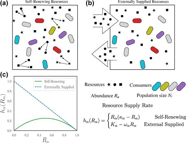
The basic intuition behind this bound is that the growth rates g_i(R) of all coexisting species i = 1,2,... must simultaneously vanish, and since the space of resource concentrations R is M-dimensional, at most M of these equations can be simultaneously solved (see Supplemental Material(SM) for discussion of non-generic phenomena where the bound is violated). While this result gives an upper bound, it is not clear when and if it will be saturated. In particular, we show below that the choice of resource dynamics fundamentally alters species-packing properties. To show this, we analyze GCRMs with two different resource dynamics: self-renewing resources where resources grow logistically in the absence of consumers [18, 19] and externally supplied resources that are supplied and degraded at a constant rate [22– 24] (see Fig. 1). We derive species packing bounds for both choices of dynamics by analyzing the susceptibilities of a new cavity solution for GCRMs with externally supplied resources and combining it with the previously derived cavity solution for GCRMs with self-renewing resources [6, 25, 26]. Surprisingly, in the absence of metabolic tradeoffs we find that, for externally-supplied resources, species can occupy only half of all available resource niches: $\frac{S^{*}}{M}<\frac{1}{2}$. Motivated by these results, we suggest a new schema for classifying ecosystems based on their species packing properties.

FIG. 1.

Schematic description for two types of resources. (a) Self-renewing resources (e.g. plants), which are replenished through organic reproduction; (b) Externally supplied resources (e.g. nutrients that sustain gut microbiota), which are replenished by a constant flux from some external source, and diluted at a constant rate; (c) The supply rate as a function of resource abundance for both choices, with κ = ω_α = K_α = 1.

Model:

GCRMs describe the ecological dynamics of S species of consumers N_i (i = 1,2,...S) that can consume M distinct resources R_α (α = 1,2,...,M). The rate at which species N_i consumes and depletes resource R_β is encoded in a matrix of consumer preferences C_iβ. In order to survive, species have a minimum maintenance cost m_i. Equivalently, m_i can also be thought of as the death rate of species i in the absence of resources. These dynamics can be described using a coupled set of M + S ordinary differential equations of the form

$$\{\begin{array}{c}\frac{d{N}_i}{dt}=N_i\sum _{\beta }{C}_{i\beta }{R}_{\beta }-N_i{m}_i\\ \frac{d{R}_{\alpha }}{dt}=h_{\alpha }\left(R_{\alpha }\right)-\sum _j{N}_j{C}_{j\alpha }{R}_{\alpha },\end{array}$$ (1)

where h_α(R_α) a function that describes the dynamics of the resources in the absence of any consumers (see Fig. 1).

For self-renewing resources (e.g. plants, animals), the dynamics can be described using logistic growth of the form

$$h_{\alpha }\left(R_{\alpha }\right)=R_{\alpha }\left({\kappa }_{\alpha }-R_{\alpha }\right),$$ (2)

with κ the carrying capacity. While such resource dynamics is reasonable for biotic resources, abiotic resources such as minerals and small molecules cannot self-replicate and are usually supplied externally to the ecosystem ( Fig. 1(b)). A common way to model this scenario is by using linearized resource dynamics of the form

$$h_{\alpha }\left(R_{\alpha }\right)=K_{\alpha }-{\omega }_{\alpha }{R}_{\alpha }.$$ (3)

Fig. 1(c) shows a plot of these two choices. Notice that the two resource dynamics behave very differently at low resource levels. The self-renewing resources can go extinct and eventually disappear from the ecosystem while this is not true of externally supplied resources.

Recent research has shown some unexpected and interesting non-generic phenomena can appear in GCRMs in the presence of additional constraints on parameter values. A common choice of such constraints is the imposition of a “metabolic budget” on the consumer preference matrix [22, 27] tying the maintenance cost m_i to the total consumption capacity ${\sum }_{\beta }{C}_{i\beta }$ [23, 28]. These metabolic tradeoffs can be readily incorporated into the cavity calculations and have significant impacts on species packing as will be discussed below.

Cavity solution:

Recently, we derived a mean-field cavity solution for steady-state dynamics of the the GCRM with self-renewing resource dynamics in the highdimensional limit where the number of resources and species in the regional species pool is large ($S,M\gg 1$)[6, 25, 26]. The overall procedure for deriving the cavity equations for GCRM with externally supplied resource is similar to that for GCRMs with self-renewing resources and is shown in Fig. S1 in the SM. We assume the K_α and m_i are independent random normal variables with means K and m and variances ${\sigma }_K^2$ and ${\sigma }_m^2$, respectively. We also assume ω_α are independent normal variables with mean ω and variance ${\sigma }_{\omega }^2$. The elements of the consumption matrix C_iα are drawn independently from a normal distribution with mean μ/M and variance ${\sigma }_c^2/M$. This scaling with M is necessary to guarantee that $\langle N\rangle ,\langle R\rangle$ do not vanish when $S,M\gg 1$ with M/S = γ fixed. Later, we will consider a slightly modified scenario where the maintenance costs are correlated with the consumption matrix in order to implement the metabolic tradeoffs discussed above.

The basic idea behind the cavity method is to derive self-consistency equations relating an ecosystem with M resources and S species to an ecosystem with M +1 resources and S + 1 resources. This is done by adding a new “cavity” species 0 and a new “cavity” resource 0 to the original ecosystem. When $S,M\gg 1$ the effect of the new cavity species/resource is small and can be treated using perturbation theory. The cavity solution further exploits the fact that since the C_iα are random variables, when $M\gg 1$ the sum ${\sum }_{\alpha }{C}_{i\alpha }{R}_{\alpha }$ will be well described by a by a normal distribution with mean μ(R) and variance ${\sigma }_c^2{q}_R$ where $q_R=\langle R^2\rangle =1/M{\sum }_{\alpha }{R}_{\alpha }^2$ (see SM for details). Combining this with the non-negativity constraint, the species distribution can be expressed as a truncated normal distribution,

$$\overline{N}=\max \left[0,\frac{\mu \langle R\rangle -m+\sqrt{{\sigma }_c^2{q}_R+{\sigma }_m^2}{z}_N}{{\sigma }_c^2\chi }\right]$$ (4)

where $\chi =-\langle \frac{\partial {\overline{R}}_{\alpha }}{\partial {\omega }_{\alpha }}\rangle =-M^{-1}{\sum }_{\alpha }\frac{\partial {\overline{R}}_{\alpha }}{\partial {\omega }_{\alpha }}$ and z_N is a standard normal variable. This equation describes GCRMs with both externally supplied and self-renewing resource dynamics [25].

The steady-state cavity equations for externally supplied resources are significantly more complicated and technically difficult to work with than the corresponding equations for self-renewing resources. To see this, no-tice that the steady-state abundance of resource α can be found by plugging in Eq. 3 into Eq 1 and setting the left hand side to zero to get

$${\overline{R}}_{\alpha }=K_{\alpha }/\left({\omega }_{\alpha }+\sum _j{\overline{N}}_j{C}_{j\alpha }\right)=\frac{K_{\alpha }}{{\omega }_{\alpha }^{\text{eff}}},$$ (5)

where we have defined ${\omega }_{\alpha }^{\text{eff}}={\omega }_{\alpha }+{\sum }_j{\overline{N}}_j{C}_{j\alpha }$. When $S,M\gg 1$, both the denominator ${\omega }_{\alpha }^{\text{eff}}$ and the numerator K_α can be modeled by independent normal random variables. This implies that the the steady-state resource abundance is described by a ratio of normal variables (i.e. the Normal Ratio Distribution) instead of a truncated Gaussian as in the self-renewing case [29](see Fig. S5). At large σ_c, this makes solving the cavity equations analytically intractable. Luckily, if the variance of the denominator ${\omega }_{\alpha }^{\text{eff}}$ is small compared with the mean – which is true when σ_c not too large – we can still obtain an approximate replica-symmetric solution by expanding in powers of the standard deviation over the mean of ${\omega }_{\alpha }^{\text{eff}}$ (see SM). We consider expansions to the cavity solutions where the denominator in Eq. 5 is expanded to 1^st order. In general, the backreaction correction is quite involved since resources and species form loopy interactions resulting in non-trivial correlation between C_iα and N_i that must be properly accounted for (see SM).

Comparison with numerics:

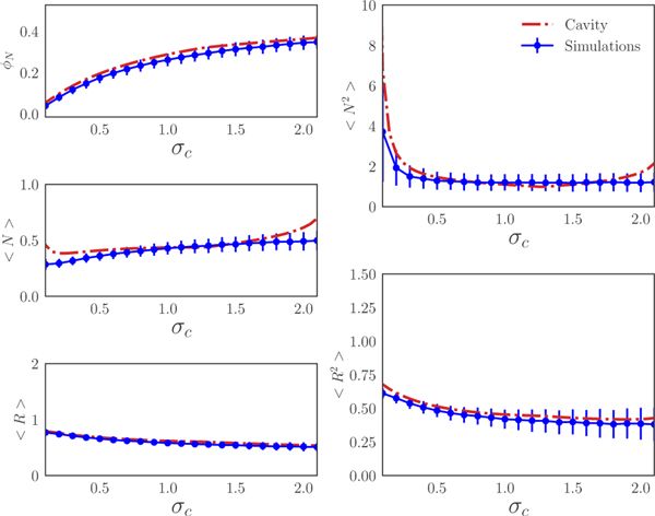
The full derivation of 1^st order expansions of the mean-field equations are given in the SM. The resulting self-consistency equations can be solved numerically in Mathematica. Fig. 2 shows a comparison between the cavity solution and 1000 independent numerical simulations for various ecosystem properties such as the fraction of surviving species S*/S and the first and second moment of the species and resource distributions (simulation details are in the SM). As can be seen in the figure, our analytic expressions agree remarkably well over a large range of σ_c. However, at very large σ_c (not shown), the cavity solutions start deviating from the numerical simulations because the Ratio Normal Distribution can no longer be described using the 1^st order expansion to the full cavity equations.

FIG. 2.

Comparison between cavity solutions (see main text for definition) and simulations for the fraction of surviving species ${\varphi }_N=\frac{S^{*}}{S}$ and the first and second moments of the species and resources distributions as a function of σ_c. The error bar shows the standard deviation from 1000 numerical simulations with M = S =100 and all other parameters are defined in the SM. Simulations were run using the CVXPY package [30].

As a further check on our analytic solution, we ran simulations where the C_iα were drawn from different distributions. One pathology of choosing C_iα from a Gaussian distribution is that when σ_c is large, many of consumption coefficients are negative. To test whether our cavity solution still describes ecosystems when C_iα are strictly positive, we compare our cavity solution to simulations where the C_iα are drawn from a Bernoulli or uniform distribution. As before, there is remarkable agreement between analytics and numerics (see Fig. S2)

Species packing without metabolic tradeoffs:

The essential ingredients needed to derive species packing bounds for GCRMS are the cavity equations for the average local susceptibilities $\nu =\langle \frac{\partial {\overline{N}}_i}{\partial m_i}\rangle =S^{-1}{\sum }_j\frac{\partial {\overline{N}}_i}{\partial m_i}$ and $\chi =\langle \frac{\partial {\overline{R}}_{\alpha }}{\partial X_{\alpha }}\rangle =M^{-1}\frac{\partial {\overline{R}}_{\alpha }}{\partial X_{\alpha }}$, with X_α = K_α for externally supplied resources and X_α = −ω_α for self-renewing resources. These two susceptibilities measure how the mean species abundance and mean resource abundance respond to changes in the species death rate and the resource supply/depletion rate, respectively. They play an essential role in the cavity equation and can be used for distinguishing different phases in complex systems[6, 31].

For the self-renewing case, the susceptibilities χ_s and ν_s are given by eq. (59, 60) in [26]

$${\nu }_s=-\frac{{\varphi }_N}{{\sigma }_c^2{\chi }_s},{\chi }_s=\frac{{\varphi }_R}{1-{\gamma }^{-1}{\sigma }_c^2{\nu }_s},$$ (6)

and can be reduced to ${\chi }_s={\varphi }_R-{\gamma }^{-1}{\varphi }_N$, where ϕ_R = M*/M, with M* equal to the number of non-extinct resources in the ecosystem. In order to guarantee the positivity of $\langle N\rangle$, we must have ${\chi }_s={\varphi }_R-{\gamma }^{-1}{\varphi }_N>0$, resulting in an upper bound

$$1\ge \frac{M^{*}}{M}>\frac{S^{*}}{M}$$ (7)

which states that the number of surviving resources must be larger than the number of surviving species.

For the externally supplied case, the corresponding equations take the form

$$\nu =-\frac{{\varphi }_N}{{\sigma }_c^2\chi },\chi =-\frac{1}{2{\gamma }^{-1}\nu {\sigma }_c^2}(1-\langle \dots \rangle ),$$ (8)

where the full expression of $\langle \dots \rangle$ can be found in eq. (63) in the SM. For our purposes, the most important property is that in the absence of metabolic tradeoffs, the expression $\langle \dots \rangle$ is always positive. Combining this observation with the equations above gives the upper bound

$$\frac{1}{2}>\frac{S^{*}}{M}={\varphi }_N{\gamma }^{-1}.$$ (9)

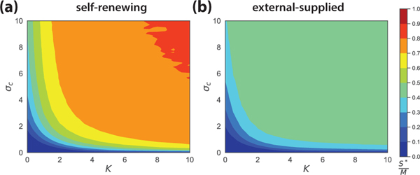
Thus, for externally supplied resources, at most half of all potential niches are occupied. Fig. 3 shows numerical simulations confirming the species packing bound for various choices of K and σ_c (see Fig. S6 in SM for various choices of S/M). The lower diversity found when resources are supplied externally can be anticipated by noting that the resource abundance in this model is more narrowly distributed than in a model with self-renewing resources. As a result, species experience stronger competition (see Fig. S5 and more details in SM). However, we still currently lack an intuitive explanation of why the species packing bound is exactly 0.5.

FIG. 3.

Comparison of the species packing ratio $\frac{S^{*}}{M}$ at various σ_c and K for self-renewing and externally supplied resource dynamics. The simulations represent averages from 1000 independent realizations with the system size M =100, S =500 (parameters in SM).

Species packing with metabolic tradeoffs:

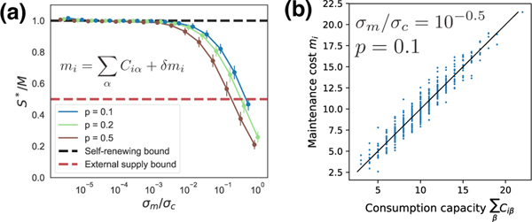
We also find that metabolic tradeoffs modify the cavity equations in such a way that the expression in brackets $\langle \dots \rangle$ in Equation (8) can become negative (see SM). However, it still remains greater than −1, allowing us to derive a species packing bound of the form S* < M even in the presence of soft metabolic constraints. In Figure 4, we simulated various ecosystems where the maintenance costs of species were chosen to obey metabolic tradeoffs of the form $m_i={\sum }_{\alpha }{C}_{i\alpha }+\delta m_i$, where δm_i are i.i.d. normal variables with variance ${\sigma }_m^2$. Note that a larger σ_m corresponds to ecosystems with softer metabolic constraints. We found that when σ_m/σ_c > 1, these ecosystems obey the 1/2 species packing bound derived above. This can also be analytically shown using the modified cavity equations derived in the SM. Finally, we show in the SM that when the metabolic tradeoffs take the form of hard constraints on the consumer preferences as in [22, 23, 27, 28], the cavity equations allow for interesting non-generic behavior with S* ≥ M, consistent with these previous works. Importantly, we find that even modest modifications of the tradeoff equation $m_i\propto {\sum }_{\alpha }{C}_{i\alpha }$ results in ecosystems that satisfy the 1/2 species packing bound.

FIG. 4.

Species packing bounds in the presence of metabolic tradeoffs. (a) The species packing ratio S*/M as a function of σ_m/σ_m, where σ_m is the standard deviation of the $\delta m_i$ and ${\sigma }_c/\sqrt{M}$ is the standard deviation of C_iα. Simulations are for binary consumer preference matrix C_iα drawn from a Bernoulli distribution with probability p. (b) m_i versus ${\sum }_{\alpha }{C}_{i\alpha }$ for p = 0.1 and σ_m/σ_c = 10^−0.5 See SM for all parameters.

Classifying ecosystems using species packing:

Recently, it has become clear that there is a deep relationship between ecosystem and constraint satisfaction problems [23, 24, 26, 28]. In particular, each species can be thought of as a constraint on possible resource abundances [24, 26]. Inspired by jamming [32], this suggests that we can separate ecosystems into qualitatively distinct classes depending on whether the competitive exclusion bound is saturated. We designate ecosystems where S* → M (like GCRMs with self-renewing resources) as isostatic species packings, and ecosystems where the upper bound S_max on the number of surviving species is strictly less than the number of resources S* < S_max < M (like GCRMs with externally supplied resources without metabolic tradeoffs) as hypostatic species packings. Ecosystems with S* ≥ M (like GCRMs with hard metabolic constraints) are designated as non-generic species packings because of the presence of a macroscopic number of additional hards constraints (i.e. the number of additional constraints that are imposed scales with S and M in the limit S,M → ∞). This basic schema suggests a way of refining the competitive exclusion principle and may help shed light on controversies surrounding the validity of basic species packing bounds.

Discussion:

In this paper, we examine the effect of resource dynamics on community structure and largescale ecosystem level properties. To do so, we analyzed generalized Consumer Resource Models (GCRMs) with two different resource dynamics: externally supplied resources that are supplied and degraded at a constant rate and self-replicating resources whose behavior in the absence of consumers is well described by a logistic growth law. Using a new cavity solution for GCRMs with externally supplied resources and a previously found cavity solution of the GCRM with self-renewing resources, we show that the community structure is fundamentally altered by the choice of resource dynamics. In particular, for externally supplied resources, we find that species generically can only occupy half of all available niches whereas for self-renewing resources all environmental niches can be filled. We confirm this surprising bound using numerical simulations.

In this manuscript, we consider the effect of metabolic trade-offs and show that they can increase species packing in an ecosystem. In the future, it will be interesting to ask how other specialized network structures, including niche partitioning, higher specialization, or combinations of specialists and generalists can affect our results. Based on our experience, we expect that, even in these more complicated ecosystems our species packing bound will hold quite generically. But much more work needs to be done to confirm if this is really the case.

Our results show how resource dynamics, which are neglected in commonly used Lotka-Volterra models, can fundamentally alter the properties of ecosystems. Much work still needs to be done to see if and how our results must be modified to account for other ecological processes such as demographic stochasticity, spatial structure, and microbe-specific interactions such as cross-feeding [7, 8]. It will also be necessary to move beyond steady-states and consider the dynamical properties of these ecosystems. More generally, it will be interesting to further explore the idea that we can classify ecosystems based on species-packing properties and see if such a schema can help us better understand the origins of the incredible diversity we observe in real-world ecosystems.

References

- [1].Huttenhower C, Gevers D, Knight R, Abubucker S, Badger JH, Chinwalla AT, Creasy HH, Earl AM, FitzGerald MG, Fulton RS, et al. , Nature 486, 207 (2012).22699609 [Google Scholar]
- [2].Gentry AH, Proceedings of the National Academy of Sciences 85, 156 (1988). [DOI] [PMC free article] [PubMed] [Google Scholar]
- [3].Mézard M, Parisi G, and Virasoro M, Spin glass theory and beyond: An Introduction to the Replica Method and Its Applications, Vol. 9 (World Scientific Publishing Company, 1987). [Google Scholar]
- [4].Nishimori H, Statistical physics of spin glasses and information processing: an introduction, 111 (Clarendon Press, 2001). [Google Scholar]
- [5].Barbier M, Arnoldi J-F, Bunin G, and Loreau M, Proceedings of the National Academy of Sciences 115, 2156 (2018). [DOI] [PMC free article] [PubMed] [Google Scholar]
- [6].Cui W, Marsland III R, and Mehta P, arXiv preprint arXiv:1904.02610 (2019).
- [7].Goldford JE, Lu N, Bajić D, Estrela S, Tikhonov M, Sanchez-Gorostiaga A, Segrè D, Mehta P, and Sanchez A, Science 361, 469 (2018). [DOI] [PMC free article] [PubMed] [Google Scholar]
- [8].Marsland III R, Cui W, Goldford J, Sanchez A, Korolev K, and Mehta P, PLoS computational biology 15, e1006793 (2019). [DOI] [PMC free article] [PubMed] [Google Scholar]
- [9].Marsland III R, Cui W, and Mehta P, arXiv preprint arXiv:1904.12914 (2019).
- [10].Fisher CK and Mehta P, Proceedings of the National Academy of Sciences 111, 13111 (2014). [DOI] [PMC free article] [PubMed] [Google Scholar]
- [11].Kessler DA and Shnerb NM, Physical Review E 91, 042705 (2015). [DOI] [PubMed] [Google Scholar]
- [12].Bunin G, Physical Review E 95, 042414 (2017). [DOI] [PubMed] [Google Scholar]
- [13].Barbier M and Arnoldi J-F, bioRxiv preprint bioRxiv: 10.1101/147728 (2017). [DOI]
- [14].Biroli G, Bunin G, and Cammarota C, New Journal of Physics 20, 083051 (2018). [Google Scholar]
- [15].Roy F, Biroli G, Bunin G, and Cammarota C, Journal of Physics A: Mathematical and Theoretical (2019).
- [16].Pearce MT, Agarwala A, and Fisher DS, bioRxiv, 736215 (2019).
- [17].Chesson P, Annual review of Ecology and Systematics 31, 343 (2000). [Google Scholar]
- [18].MacArthur R and Levins R, The American Naturalist 101, 377 (1967). [Google Scholar]
- [19].Chesson P, Theoretical Population Biology 37, 26 (1990). [DOI] [PubMed] [Google Scholar]
- [20].MacArthur R, Theoretical population biology 1, 1 (1970). [DOI] [PubMed] [Google Scholar]
- [21].McGehee R and Armstrong RA, Journal of Differential Equations 23, 30 (1977). [Google Scholar]
- [22].Posfai A, Taillefumier T, and Wingreen NS, Physical review letters 118, 028103 (2017). [DOI] [PMC free article] [PubMed] [Google Scholar]
- [23].Tikhonov M and Monasson R, Physical review letters 118, 048103 (2017). [DOI] [PubMed] [Google Scholar]
- [24].Marsland III R, Cui W, and Mehta P, arXiv preprint arXiv:1901.09673 (2019).
- [25].Advani M, Bunin G, and Mehta P, Journal of Statistical Mechanics: Theory and Experiment, 033406 (2018). [DOI] [PMC free article] [PubMed]
- [26].Mehta P, Cui W, Wang C-H, and Marsland III R, Physical Review E 99, 052111 (2019). [DOI] [PMC free article] [PubMed] [Google Scholar]
- [27].Li Z, Liu B, Li SH-J, King CG, Gitai Z, and Wingreen NS, bioRxiv, 664698 (2019).
- [28].Altieri A and Franz S, Physical Review E 99, 010401 (2019). [DOI] [PubMed] [Google Scholar]
- [29].Marsaglia G et al. , Journal of Statistical Software 16, 1 (2006). [Google Scholar]
- [30].Agrawal A, Verschueren R, Diamond S, and Boyd S, Journal of Control and Decision 5, 42 (2018). [Google Scholar]
- [31].Ramezanali M, Mitra PP, and Sengupta AM, arXiv preprint arXiv:1501.03194 (2015).
- [32].Liu AJ and Nagel SR, Annu. Rev. Condens. Matter Phys. 1, 347 (2010). [Google Scholar]
Associated Data
This section collects any data citations, data availability statements, or supplementary materials included in this article.